Probabilistic Program Equivalence for NetKAT

Abstract.

We tackle the problem of deciding whether two probabilistic programs are equivalent in Probabilistic NetKAT, a formal language for specifying and reasoning about the behavior of packet-switched networks. We show that the problem is decidable for the history-free fragment of the language by developing an effective decision procedure based on stochastic matrices. The main challenge lies in reasoning about iteration, which we address by designing an encoding of the program semantics as a finite-state absorbing Markov chain, whose limiting distribution can be computed exactly. In an extended case study on a real-world data center network, we automatically verify various quantitative properties of interest, including resilience in the presence of failures, by analyzing the Markov chain semantics.

1. Introduction

Program equivalence is one of the most fundamental problems in Computer Science: given a pair of programs, do they describe the same computation? The problem is undecidable in general, but it can often be solved for domain-specific languages based on restricted computational models. For example, a classical approach for deciding whether a pair of regular expressions denote the same language is to first convert the expressions to deterministic finite automata, which can then be checked for equivalence in almost linear time (Tarjan, 1975). In addition to the theoretical motivation, there are also many practical benefits to studying program equivalence. Being able to decide equivalence enables more sophisticated applications, for instance in verified compilation and program synthesis. Less obviously—but arguably more importantly—deciding equivalence typically involves finding some sort of finite, explicit representation of the program semantics. This compact encoding can open the door to reasoning techniques and decision procedures for properties that extend far beyond straightforward program equivalence.

With this motivation in mind, this paper tackles the problem of deciding equivalence in Probabilistic NetKAT (ProbNetKAT), a language for modeling and reasoning about the behavior of packet-switched networks. As its name suggests, ProbNetKAT is based on NetKAT (Anderson et al., 2014; Foster et al., 2015; Smolka et al., 2015), which is in turn based on Kleene algebra with tests (KAT), an algebraic system combining Boolean predicates and regular expressions. ProbNetKAT extends NetKAT with a random choice operator and a semantics based on Markov kernels (Smolka et al., 2017). The framework can be used to encode and reason about randomized protocols (e.g., a routing scheme that uses random forwarding paths to balance load (Valiant, 1982)); describe uncertainty about traffic demands (e.g., the diurnal/nocturnal fluctuation in access patterns commonly seen in networks for large content providers (Roy et al., 2015)); and model failures (e.g., switches or links that are known to fail with some probability (Gill et al., 2011)).

However, the semantics of ProbNetKAT is surprisingly subtle. Using the iteration operator (i.e., the Kleene star from regular expressions), it is possible to write programs that generate continuous distributions over an uncountable space of packet history sets (Foster et al., 2016, Theorem 3). This makes reasoning about convergence non-trivial, and requires representing infinitary objects compactly in an implementation. To address these issues, prior work (Smolka et al., 2017) developed a domain-theoretic characterization of ProbNetKAT that provides notions of approximation and continuity, which can be used to reason about programs using only discrete distributions with finite support. However, that work left the decidability of program equivalence as an open problem. In this paper, we settle this question positively for the history-free fragment of the language, where programs manipulate sets of packets instead of sets of packet histories (finite sequences of packets).

Our decision procedure works by deriving a canonical, explicit representation of the program semantics, for which checking equivalence is straightforward. Specifically, we define a big-step semantics that interprets each program as a finite stochastic matrix—equivalently, a Markov chain that transitions from input to output in a single step. Equivalence is trivially decidable on this representation, but the challenge lies in computing the big-step matrix for iteration—intuitively, the finite matrix needs to somehow capture the result of an infinite stochastic process. We address this by embedding the system in a more refined Markov chain with a larger state space, modeling iteration in the style of a small-step semantics. With some care, this chain can be transformed to an absorbing Markov chain, from which we derive a closed form analytic solution representing the limit of the iteration by applying elementary matrix calculations. We prove the soundness of this approach formally.

Although the history-free fragment of ProbNetKAT is a restriction of the general language, it captures the input-output behavior of a network—mapping initial packet states to final packet states—and is still expressive enough to handle a wide range of problems of interest. Many other contemporary network verification tools, including Anteater (Mai et al., 2011), Header Space Analysis (Kazemian et al., 2012), and Veriflow (Khurshid et al., 2012), are also based on a history-free model. To handle properties that involve paths (e.g., waypointing), these tools generate a series of smaller properties to check, one for each hop in the path. In the ProbNetKAT implementation, working with history-free programs can reduce the space requirements by an exponential factor—a significant benefit when analyzing complex randomized protocols in large networks.

We have built a prototype implementation of our approach in OCaml. The workhorse of the decision procedure computes a finite stochastic matrix—representing a finite Markov chain—given an input program. It leverages the spare linear solver UMFPACK (Davis, 2004) as a back-end to compute limiting distributions, and incorporates a number of optimizations and symbolic techniques to compactly represent large but sparse matrices. Although building a scalable implementation would require much more engineering (and is not the primary focus of this paper), our prototype is already able to handle programs of moderate size. Leveraging the finite encoding of the semantics, we have carried out several case studies in the context of data center networks; our central case study models and verifies the resilience of various routing schemes in the presence of link failures.

Contributions and outline.

The main contribution of this paper is the development of a decision procedure for history-free ProbNetKAT. We develop a new, tractable semantics in terms of stochastic matrices in two steps, we establish the soundness of the semantics with respect to ProbNetKAT’s original denotational model, and we use the compact semantics as the basis for building a prototype implementation with which we carry out case studies.

In Section 2 and Section 3 we introduce ProbNetKAT using a simple example and motivate the need for quantitative, probabilistic reasoning.

In Section 4, we present a semantics based on finite stochastic matrices and show that it fully characterizes the behavior of ProbNetKAT programs on packets (Theorem 4.1). In this big-step semantics, the matrices encode Markov chains over the state space $2^{\mathsf{Pk}}$. A single step of the chain models the entire execution of a program, going directly from the initial state corresponding to the set of input packets the final state corresponding to the set of output packets. Although this reduces program equivalence to equality of finite matrices, we still need to provide a way to explicitly compute them. In particular, the matrix that models iteration is given in terms of a limit.

In Section 5 we derive a closed form for the big-step matrix associated with $p^{*}$, giving an explicit representation of the big-step semantics. It is important to note that this is not simply the calculation of the stationary distribution of a Markov chain, as the semantics of $p^{*}$ is more subtle. Instead, we define a small-step semantics, a second Markov chain with a larger state space such that one transition models one iteration of $p^{*}$. We then show how to transform this finer Markov chain into an absorbing Markov chain, which admits a closed form solution for its limiting distribution. Together, the big- and small-step semantics enable us to analytically compute a finite representation of the program semantics. Directly checking these semantics for equality yields an effective decision procedure for program equivalence (Corollary 5.8). This is in contrast with the previous semantics (Foster et al., 2016), which merely provided an approximation theorem for the semantics of iteration $p^{*}$ and was not suitable for deciding equivalence.

In Section 6, we illustrate the practical applicability of our approach by exploiting the representation of ProbNetKAT programs as stochastic matrices to answer a number of questions of interest in real-world networks. For example, we can reduce loop termination to program equivalence: the fact that the while loop below terminates with probability $1$ can be checked as follows:

$$\mathsf{while}~{}\neg\mathit{f}\kern 0.43057pt{=}\kern 0.43057pt0~{}\mathsf{do}~{}(\mathsf{skip}\mathop{\mathrel{\oplus_{r}}}\mathit{f}\kern 0.43057pt{\leftarrow}\kern 0.43057pt0)\quad\equiv\quad\mathit{f}\kern 0.43057pt{\leftarrow}\kern 0.43057pt0$$

We also present real-world case studies that use the stochastic matrix representation to answer questions about the resilience of data center networks in the presence of link failures.

We discuss obstacles in extending our approach to the full ProbNetKAT language in Section 7, including a novel automata model encodable in ProbNetKAT for which equivalence seems challenging to decide. We survey related work in Section 8 and conclude in Section 9.

2. Overview

This section introduces the syntax and semantics of ProbNetKAT using a simple example. We will also see how various properties, including program equivalence and also program ordering and quantitative computations over the output distribution, can be encoded in ProbNetKAT. Each of the analyses in this section can be automatically carried out in our prototype implementation.

As our running example, consider the network shown in Figure 1. It connects Source and Destination hosts through a topology with three switches. Suppose we want to implement the following policy: forward packets from the Source to the Destination. We will start by building a straightforward implementation of this policy in ProbNetKAT and then verify that it correctly implements the specification embodied in the policy using program equivalence. Next, we will refine our implementation to improve its resilience to link failures and verify that the refinement is more resilient. Finally, we characterize the resilience of both implementations quantitatively.

2.1. Deterministic Programming and Reasoning

We will start with a simple deterministic program that forwards packets from left to right through the topology. To a first approximation, a ProbNetKAT program can be thought of as a random function from input packets to output packets. We model packets as records, with fields for standard headers such as the source address ($\mathsf{src}$) and destination address ($\mathsf{dst}$) of a packet, as well as two fields switch ($\mathsf{sw}$) and port ($\mathsf{pt}$) identifying the current location of the packet. The precise field names and ranges turns out to be not so important for our purposes; what is crucial is that the number of fields and the size of their domains must be finite.

NetKAT provides primitives $\mathit{f}\kern 0.43057pt{\leftarrow}\kern 0.43057ptn$ and $\mathit{f}\kern 0.43057pt{=}\kern 0.43057ptn$ to modify and test the field $\mathit{f}$ of an incoming packet. A modification $\mathit{f}\kern 0.43057pt{\leftarrow}\kern 0.43057ptn$ returns the input packet with the $\mathit{f}$ field updated to $n$. A test $\mathit{f}\kern 0.43057pt{=}\kern 0.43057ptn$ either returns the input packet unmodified if the test succeeds, or returns the empty set if the test fails. There are also primitives $\mathsf{skip}$ and $\mathsf{drop}$ that behave like a test that always succeeds and fails, respectively. Programs $p,q$ are assembled to larger programs by composing them in sequence ($p\mathbin{;}q$) or in parallel ($p\mathbin{\scalebox{1.0}[1.15]{\&}}q$). NetKAT also provides the Kleene star operator $p^{*}$ from regular expressions to iterate programs. ProbNetKAT extends NetKAT with an additional operator $p\oplus_{r}q$ that executes either $p$ with probability $r$, or $q$ with probability $1-r$.

Forwarding.

We now turn to the implementation of our forwarding policy. To route packets from Source to Destination, all switches can simply forward incoming packets out of port 2:

$$p_{1}\mathrel{\smash{\triangleq}}\mathsf{pt}\kern 0.43057pt{\leftarrow}\kern 0.43057pt2 p_{2}\mathrel{\smash{\triangleq}}\mathsf{pt}\kern 0.43057pt{\leftarrow}\kern 0.43057pt2 p_{3}\mathrel{\smash{\triangleq}}\mathsf{pt}\kern 0.43057pt{\leftarrow}\kern 0.43057pt2$$

This is achieved by modifying the port field $(\mathsf{pt})$. Then, to encode the forwarding logic for all switches into a single program, we take the union of their individual programs, after guarding the policy for each switch with a test that matches packets at that switch:

$$p\mathrel{\smash{\triangleq}}(\mathsf{sw}\kern 0.43057pt{=}\kern 0.43057pt1\mathbin{;}p_{1})~{}\mathbin{\scalebox{1.0}[1.15]{\&}}~{}(\mathsf{sw}\kern 0.43057pt{=}\kern 0.43057pt2\mathbin{;}p_{2})~{}\mathbin{\scalebox{1.0}[1.15]{\&}}~{}(sw\kern 0.43057pt{=}\kern 0.43057pt3\mathbin{;}p_{3})$$

Note that we specify a policy for switch 3, even though it is unreachable.

Now we would like to answer the following question: does our program $p$ correctly forward packets from Source to Destination? Note however that we cannot answer the question by inspecting $p$ alone, since the answer depends fundamentally on the network topology.

Figure 1. Example network.

Topology.

Although the network topology is not programmable, we can still model its behavior as a program. A unidirectional link matches on packets located at the source location of the link, and updates their location to the destination of the link. In our example network (Figure 1), the link $\ell_{ij}$ from switch $i$ to switch $j\neq i$ is given by

$$\ell_{ij} \mathrel{\smash{\triangleq}}\mathsf{sw}\kern 0.43057pt{=}\kern 0.43057pti\mathbin{;}\mathsf{pt}\kern 0.43057pt{=}\kern 0.43057ptj\mathbin{;}\mathsf{sw}\kern 0.43057pt{\leftarrow}\kern 0.43057ptj\mathbin{;}\mathsf{pt}\kern 0.43057pt{\leftarrow}\kern 0.43057pti$$

We obtain a model for the entire topology by taking the union of all its links:

$$t \mathrel{\smash{\triangleq}}\ell_{12}\mathbin{\scalebox{1.0}[1.15]{\&}}\ell_{13}\mathbin{\scalebox{1.0}[1.15]{\&}}\ell_{32}$$

Although this example uses unidirectional links, bidirectional links can be modeled as well using a pair of unidirectional links.

Network Model.

A packet traversing the network is subject to an interleaving of processing steps by switches and links in the network. This is expressible in NetKAT using Kleene star as follows:

$$\operatorname{M}(p,t)\mathrel{\smash{\triangleq}}(p\mathbin{;}t)^{*}\mathbin{;}p$$

However, the model $\operatorname{M}(p,t)$ captures the behavior of the network on arbitrary input packets, including packets that start at arbitrary locations in the interior of the network. Typically we are interested only in the behavior of the network for packets that originate at the ingress of the network and arrive at the egress of the network. To restrict the model to such packets, we can define predicates $in$ and $out$ and pre- and post-compose the model with them:

$$in\mathbin{;}\operatorname{M}(p,t)\mathbin{;}out$$

For our example network, we are interested in packets originating at the Source and arriving at the Destination, so we define

$$in\mathrel{\smash{\triangleq}}\mathsf{sw}\kern 0.43057pt{=}\kern 0.43057pt1\mathbin{;}\mathsf{pt}\kern 0.43057pt{=}\kern 0.43057pt1 out\mathrel{\smash{\triangleq}}\mathsf{sw}\kern 0.43057pt{=}\kern 0.43057pt2\mathbin{;}\mathsf{pt}\kern 0.43057pt{=}\kern 0.43057pt2$$

With a full network model in hand, we can verify that $p$ correctly implements the desired network policy, i.e. forward packets from Source to Destination. Our informal policy can be expressed formally as a simple ProbNetKAT program:

$$\mathit{teleport}\mathrel{\smash{\triangleq}}\mathsf{sw}\kern 0.43057pt{\leftarrow}\kern 0.43057pt2\mathbin{;}\mathsf{pt}\kern 0.43057pt{\leftarrow}\kern 0.43057pt2$$

We can then settle the correctness question by checking the equivalence

$$in\mathbin{;}\operatorname{M}(p,t)\mathbin{;}out\ \equiv\ in\mathbin{;}\mathit{teleport}$$

Previous work (Anderson et al., 2014; Foster et al., 2015; Smolka et al., 2015) used NetKAT equivalence with similar encodings to reason about various essential network properties including waypointing, reachability, isolation, and loop freedom, as well as for the validation and verification of compiler transformations. Unfortunately, the NetKAT decision procedure (Foster et al., 2015) and other state of the art network verification tools (Kazemian et al., 2012; Khurshid et al., 2012) are fundamentally limited to reasoning about deterministic network behaviors.

2.2. Probabilistic Programming and Reasoning

Routing schemes used in practice often behave non-deterministically—e.g., they may distribute packets across multiple paths to avoid congestion, or they may switch to backup paths in reaction to failures. To see these sorts of behaviors in action, let’s refine our naive routing scheme $p$ to make it resilient to random link failures.

Link Failures.

We will assume that switches have access to a boolean flag $\mathsf{up_{i}}$ that is true if and only if the link connected to the switch at port $i$ is transmitting packets correctly. To make the network resilient to a failure, we can modify the program for Switch 1 as follows: if the link $\ell_{12}$ is up, use the shortest path to Switch 2 as before; otherwise, take a detour via Switch 3, which still forwards all packets to Switch 2.

$$\widehat{p}_{1}\mathrel{\smash{\triangleq}}(\mathsf{up_{2}}\kern 0.43057pt{=}\kern 0.43057pt1\mathbin{;}\mathsf{pt}\kern 0.43057pt{\leftarrow}\kern 0.43057pt2)\mathbin{\scalebox{1.0}[1.15]{\&}}(\mathsf{up_{2}}\kern 0.43057pt{=}\kern 0.43057pt0\mathbin{;}\mathsf{pt}\kern 0.43057pt{\leftarrow}\kern 0.43057pt3)$$

As before, we can then encode the forwarding logic for all switches into a single program:

$$\widehat{p} \mathrel{\smash{\triangleq}}(\mathsf{sw}\kern 0.43057pt{=}\kern 0.43057pt1\mathbin{;}\widehat{p_{1}})~{}\mathbin{\scalebox{1.0}[1.15]{\&}}~{}(\mathsf{sw}\kern 0.43057pt{=}\kern 0.43057pt2\mathbin{;}p_{2})~{}\mathbin{\scalebox{1.0}[1.15]{\&}}~{}(\mathsf{sw}\kern 0.43057pt{=}\kern 0.43057pt3\mathbin{;}p_{3})$$

Next, we update our link and topology encodings. A link behaves as before when it is up, but drops all incoming packets otherwise:

$$\widehat{\ell}_{ij} \mathrel{\smash{\triangleq}}\mathsf{up_{j}}\kern 0.43057pt{=}\kern 0.43057pt1\mathbin{;}\ell_{ij}$$

For the purposes of this example, we will consider failures of links connected to Switch $1$ only:

$$\widehat{t} \mathrel{\smash{\triangleq}}\widehat{\ell}_{12}\mathbin{\scalebox{1.0}[1.15]{\&}}\widehat{\ell}_{13}\mathbin{\scalebox{1.0}[1.15]{\&}}\ell_{32}$$

We also need to assume some failure model, i.e. a probabilistic model of when and how often links fail. We will consider three failure models:

$$f_{0} \mathrel{\smash{\triangleq}}\mathsf{up_{2}}\kern 0.43057pt{\leftarrow}\kern 0.43057pt1\mathbin{;}\mathsf{up_{3}}\kern 0.43057pt{\leftarrow}\kern 0.43057pt1$$

$$f_{1} \mathrel{\smash{\triangleq}}\bigoplus\left\{f_{0}\mathbin{@}\frac{1}{2},~{}(\mathsf{up_{2}}\kern 0.43057pt{\leftarrow}\kern 0.43057pt0)\mathbin{\scalebox{1.0}[1.15]{\&}}(\mathsf{up_{3}}\kern 0.43057pt{\leftarrow}\kern 0.43057pt1)\mathbin{@}\frac{1}{4},~{}(\mathsf{up_{2}}\kern 0.43057pt{\leftarrow}\kern 0.43057pt1)\mathbin{\scalebox{1.0}[1.15]{\&}}(\mathsf{up_{3}}\kern 0.43057pt{\leftarrow}\kern 0.43057pt0)\mathbin{@}\frac{1}{4}\right\}$$

$$f_{2} \mathrel{\smash{\triangleq}}(\mathsf{up_{2}}\kern 0.43057pt{\leftarrow}\kern 0.43057pt1\oplus_{0.8}\mathsf{up_{2}}\kern 0.43057pt{\leftarrow}\kern 0.43057pt0)\mathbin{;}(\mathsf{up_{2}}\kern 0.43057pt{\leftarrow}\kern 0.43057pt1\oplus_{0.8}\mathsf{up_{2}}\kern 0.43057pt{\leftarrow}\kern 0.43057pt0)$$

Intuitively, in model $f_{0}$, links never fail; in $f_{1}$, the links $\ell_{12}$ and $\ell_{13}$ can fail with probability $25\%$ each, but at most one fails; in $f_{2}$, the links can fail independently with probability $20\%$ each.

Finally, we can assemble the encodings of policy, topology, and failures into a refined model:

$$\widehat{\operatorname{M}}(p,t,f)\mathrel{\smash{\triangleq}}~{} \mathsf{var}~{}\mathsf{up_{2}}\kern 0.43057pt{\leftarrow}\kern 0.43057pt1~{}\mathsf{in}$$

$$\mathsf{var}~{}\mathsf{up_{3}}\kern 0.43057pt{\leftarrow}\kern 0.43057pt1~{}\mathsf{in}$$

$$\operatorname{M}((f\mathbin{;}p),t)$$

The refined model $\widehat{\operatorname{M}}$ wraps our previous model $\operatorname{M}$ with declarations of the two local variables $\mathsf{up_{2}}$ and $\mathsf{up_{3}}$, and it executes the failure model at each hop prior to switch and topology processing. As a quick sanity check, we can verify that the old model and the new model are equivalent in the absence of failures, i.e. under failure model $f_{0}$:

$$\operatorname{M}(p,t)\ \equiv\ \widehat{\operatorname{M}}(p,\widehat{t},f_{0})$$

Now let us analyze our resilient routing scheme $\widehat{p}$. First, we can verify that it correctly routes packets to the Destination in the absence of failures by checking the following equivalence:

$$in\mathbin{;}\widehat{\operatorname{M}}(\widehat{p},\widehat{t},f_{0})\mathbin{;}out\ \equiv\ in\mathbin{;}\mathit{teleport}$$

In fact, the scheme $\widehat{p}$ is 1-resilient: it delivers all packets as long as no more than $1$ link fails. In particular, it behaves like $\mathit{teleport}$ under failure model $f_{1}$. In contrast, this is not true for our naive routing scheme $p$:

$$in\mathbin{;}\widehat{\operatorname{M}}(\widehat{p},\widehat{t},f_{1})\mathbin{;}out\ \equiv\ in\mathbin{;}\mathit{teleport}\ \nequiv\ in\mathbin{;}\widehat{\operatorname{M}}(p,\widehat{t},f_{1})\mathbin{;}out$$

Under failure model $f_{2}$, neither of the routing schemes is fully resilient and equivalent to teleportation. However, it is reassuring to verify that the refined routing scheme $\widehat{p}$ performs strictly better than the naive scheme $p$,

$$\widehat{\operatorname{M}}(p,\widehat{t},f_{2})\ <\ \widehat{\operatorname{M}}(\widehat{p},\widehat{t},f_{2})$$

where $p<q$ means that $q$ delivers packets with higher probability than $p$.

Reasoning using program equivalences and inequivalences is helpful to establish qualitative properties such as reachability properties and program invariants. But we can also go a step further, and compute quantitative properties of the packet distribution generated by a ProbNetKAT program. For example, we may ask for the probability that the schemes deliver a packet originating at Source to Destination under failure model $f_{2}$. The answer is $80\%$ for the naive scheme, and $96\%$ for the resilient scheme. Such a computation might be used by an Internet Service Provider (ISP) to check that it can meet its service-level agreements (SLA) with customers.

In Section 6 we will analyze a more sophisticated resilient routing scheme and see more complex examples of qualitative and quantitative reasoning with ProbNetKAT drawn from real-world data center networks. But first, we turn to developing the theoretical foundations (Sections 3, 4 and 5).

3. Background on Probabilistic NetKAT

In this section, we review the syntax and semantics of ProbNetKAT (Smolka et al., 2017; Foster et al., 2016) and basic properties of the language, focusing on the history-free fragment. A synopsis appears in Figure 2.

3.1. Syntax

A packet $\pi$ is a record mapping a finite set of fields $\mathit{f}_{1},\mathit{f}_{2},\dots,\mathit{f}_{k}$ to bounded integers $n$. Fields include standard header fields such as source ($\mathsf{src}$) and destination ($\mathsf{dst}$) addresses, as well as two logical fields for the switch ($\mathsf{sw}$) and port ($\mathsf{pt}$) that record the current location of the packet in the network. The logical fields are not present in a physical network packet, but it is convenient to model them as if they were. We write $\pi.\mathit{f}$ to denote the value of field $\mathit{f}$ of $\pi$ and $\pi[\mathit{f}{:=}n]$ for the packet obtained from $\pi$ by updating field $\mathit{f}$ to $n$. We let $\mathsf{Pk}$ denote the (finite) set of all packets.

ProbNetKAT expressions consist of predicates ($t,u,\ldots$) and programs ($p,q,\ldots$). Primitive predicates include tests ($\mathit{f}\kern 0.43057pt{=}\kern 0.43057ptn$) and the Boolean constants false ($\mathsf{drop}$) and true ($\mathsf{skip}$). Compound predicates are formed using the usual Boolean connectives of disjunction ($t\mathbin{\scalebox{1.0}[1.15]{\&}}u$), conjunction ($t\mathbin{;}u$), and negation ($\neg t$). Primitive programs include predicates ($t$) and assignments ($\mathit{f}\kern 0.43057pt{\leftarrow}\kern 0.43057ptn$). Compound programs are formed using the operators parallel composition ($p\mathbin{\scalebox{1.0}[1.15]{\&}}q$), sequential composition ($p\mathbin{;}q$), iteration ($p^{*}$), and probabilistic choice ($p\mathrel{\oplus_{r}}q$). The full version of the language also provides a $\mathsf{dup}$ primitives, which logs the current state of the packet, but we omit this operator from the history-free fragment of the language considered in this paper; we discuss technical challenges to handling full ProbNetKAT in Section 7.

The probabilistic choice operator $p\mathrel{\oplus_{r}}q$ executes $p$ with probability $r$ and $q$ with probability $1-r$, where $r$ is rational, $0\leq r\leq 1$. We often use an $n$-ary version and omit the $r$’s as in $p_{1}\oplus\cdots\oplus p_{n}$, which is interpreted as executing one of the $p_{i}$ chosen with equal probability. This can be desugared into the binary version.

Conjunction of predicates and sequential composition of programs use the same syntax ($t\mathbin{;}u$ and $p\mathbin{;}q$, respectively), as their semantics coincide. The same is true for disjunction of predicates and parallel composition of programs ($t\mathbin{\scalebox{1.0}[1.15]{\&}}u$ and $p\mathbin{\scalebox{1.0}[1.15]{\&}}q$, respectively). The negation operator ($\neg$) may only be applied to predicates.

The language as presented in Figure 2 only includes core primitives, but many other useful constructs can be derived. In particular, it is straightforward to encode conditionals and while loops:

$$\mathsf{if}~{}t~{}\mathsf{then}~{}p~{}\mathsf{else}~{}q ~{}\mathrel{\smash{\triangleq}}~{}t\mathbin{;}p\mathbin{\scalebox{1.0}[1.15]{\&}}\neg t\mathbin{;}q \qquad\qquad\mathsf{while}~{}t~{}\mathsf{do}~{}p ~{}\mathrel{\smash{\triangleq}}~{}(t\mathbin{;}p)^{*}\mathbin{;}\neg t$$

These encodings are well known from KAT (Kozen, 1997). Mutable and immutable local variables can also be desugared into the core calculus (although our implementation supports them directly):

$$\mathsf{var}~{}\mathit{f}\kern 0.43057pt{\leftarrow}\kern 0.43057ptn~{}\mathsf{in}~{}p~{}\mathrel{\smash{\triangleq}}~{}\mathit{f}\kern 0.43057pt{\leftarrow}\kern 0.43057ptn\mathbin{;}p\mathbin{;}\mathit{f}\kern 0.43057pt{\leftarrow}\kern 0.43057pt0$$

Here $\mathit{f}$ is an otherwise unused field. The assignment $\mathit{f}\kern 0.43057pt{\leftarrow}\kern 0.43057pt0$ ensures that the final value of $\mathit{f}$ is “erased” after the field goes out of scope.

Syntax

$$\begin{array}[]{r@{\kern 1ex}r@{~}c@{~}l@{\kern 2em}l}\textrm{Naturals}\kern 4.30554pt&n~{}&::=\hfil~{}&\mathrlap{0\mid 1\mid 2\mid\cdots}\hfil\kern 20.00003pt\\ \textrm{Fields}\kern 4.30554pt&\mathit{f}~{}&::=\hfil~{}&\mathrlap{\mathit{f}_{1}\mid\cdots\mid\mathit{f}_{k}}\hfil\kern 20.00003pt\\ \textrm{Packets}\kern 4.30554pt&\mathsf{Pk}\ni\pi~{}&::=\hfil~{}&\mathrlap{\{\mathit{f}_{1}=n_{1},\dots,\mathit{f}_{k}=n_{k}\}}\hfil\kern 20.00003pt\\ \textrm{Probabilities}\kern 4.30554pt&r~{}&\in\hfil~{}&\mathrlap{[0,1]\cap\mathbb{Q}}\hfil\kern 20.00003pt\\[4.30554pt] \textrm{Predicates}\kern 4.30554pt&t,u~{}&::=\hfil~{}&\mathsf{drop}\hfil\kern 20.00003pt&\textit{False}\\ \kern 4.30554pt&~{}&\mid\hfil~{}&\mathsf{skip}\hfil\kern 20.00003pt&\textit{True}\\ \kern 4.30554pt&~{}&\mid\hfil~{}&\mathit{f}\kern 0.43057pt{=}\kern 0.43057ptn\hfil\kern 20.00003pt&\textit{Test}\\ \kern 4.30554pt&~{}&\mid\hfil~{}&t\mathbin{\scalebox{1.0}[1.15]{\&}}u\hfil\kern 20.00003pt&\textit{Disjunction}\\ \kern 4.30554pt&~{}&\mid\hfil~{}&t\mathbin{;}u\hfil\kern 20.00003pt&\textit{Conjunction}\\ \kern 4.30554pt&~{}&\mid\hfil~{}&\neg t\hfil\kern 20.00003pt&\textit{Negation}\\[4.30554pt] \textrm{Programs}\kern 4.30554pt&p,q~{}&::=\hfil~{}&t\hfil\kern 20.00003pt&\textit{Filter}\\ \kern 4.30554pt&~{}&\mid\hfil~{}&\mathit{f}\kern 0.43057pt{\leftarrow}\kern 0.43057ptn\hfil\kern 20.00003pt&\textit{Assignment}\\ \kern 4.30554pt&~{}&\mid\hfil~{}&p\mathbin{\scalebox{1.0}[1.15]{\&}}q\hfil\kern 20.00003pt&\textit{Union}\\ \kern 4.30554pt&~{}&\mid\hfil~{}&p\mathbin{;}q\hfil\kern 20.00003pt&\textit{Sequence}\\ \kern 4.30554pt&~{}&\mid\hfil~{}&p\mathrel{\oplus_{r}}q\hfil\kern 20.00003pt&\textit{Choice}\\ \kern 4.30554pt&~{}&\mid\hfil~{}&p^{*}\hfil\kern 20.00003pt&\textit{Iteration}\end{array}$$

    Semantics $\llbracket p\rrbracket\in\smash{2^{\mathsf{Pk}}}\to\operatorname{\mathcal{D}}(\smash{2^{\mathsf{Pk}}})$ $$\begin{array}[]{r@{~~}c@{~~}l}\llbracket\mathsf{drop}\rrbracket(a)~{}~{}&\mathrel{\smash{\triangleq}}\hfil~{}~{}&\delta({\varnothing})\\ \llbracket\mathsf{skip}\rrbracket(a)~{}~{}&\mathrel{\smash{\triangleq}}\hfil~{}~{}&\delta({a})\\ \llbracket\mathit{f}\kern 0.43057pt{=}\kern 0.43057ptn\rrbracket(a)~{}~{}&\mathrel{\smash{\triangleq}}\hfil~{}~{}&\delta({\{\pi\in a\mid\pi.f=n\}})\\ \llbracket\mathit{f}\kern 0.43057pt{\leftarrow}\kern 0.43057ptn\rrbracket(a)~{}~{}&\mathrel{\smash{\triangleq}}\hfil~{}~{}&\delta({\{\pi[\mathit{f}{:=}n]\mid\pi\in a\}})\\ \llbracket\neg t\rrbracket(a)~{}~{}&\mathrel{\smash{\triangleq}}\hfil~{}~{}&\operatorname{\mathcal{D}}(\lambda b.a-b)(\llbracket t\rrbracket(a))\\ \llbracket p\mathbin{\scalebox{1.0}[1.15]{\&}}q\rrbracket(a)~{}~{}&\mathrel{\smash{\triangleq}}\hfil~{}~{}&\operatorname{\mathcal{D}}(\cup)(\llbracket p\rrbracket(a)\times\llbracket q\rrbracket(a))\\ \llbracket p\mathbin{;}q\rrbracket(a)~{}~{}&\mathrel{\smash{\triangleq}}\hfil~{}~{}&\llbracket q\rrbracket^{\dagger}(\llbracket p\rrbracket(a))\\ \llbracket p\mathop{\mathrel{\oplus_{r}}}q\rrbracket(a)~{}~{}&\mathrel{\smash{\triangleq}}\hfil~{}~{}&r\cdot\llbracket p\rrbracket(a)+(1-r)\cdot\llbracket q\rrbracket(a)\\ \llbracket p^{*}\rrbracket(a)~{}~{}&\mathrel{\smash{\triangleq}}\hfil~{}~{}&\displaystyle\bigsqcup_{n\in\mathbb{N}}\llbracket p^{(n)}\rrbracket(a)\\ \lx@intercol\text{where }~{}p^{(0)}\mathrel{\smash{\triangleq}}\mathsf{skip},\hskip 6.45831ptp^{(n+1)}\mathrel{\smash{\triangleq}}\mathsf{skip}\mathbin{\scalebox{1.0}[1.15]{\&}}p\mathbin{;}p^{(n)}\hfil\lx@intercol\end{array}$$   (Discrete) Probability Monad $\operatorname{\mathcal{D}}$ $$\begin{array}[]{@{}r@{\quad}l@{}}\text{Unit}&\delta:X\to\operatorname{\mathcal{D}}(X)\quad\delta(x)\mathrel{\smash{\triangleq}}\delta_{x}\\ \text{Bind}&-^{\dagger}:(X\to\operatorname{\mathcal{D}}(Y))\to\operatorname{\mathcal{D}}(X)\to\operatorname{\mathcal{D}}(Y)\\ &f^{\dagger}(\mu)(A)\mathrel{\smash{\triangleq}}\sum_{x\in X}f(x)(A)\cdot\mu(x)\end{array}$$

Figure 2. ProbNetKAT core language: syntax and semantics.

3.2. Semantics

In the full version of ProbNetKAT, the space $\smash{2^{\mathsf{H}}}$ of sets of packet histories is uncountable, and programs can generate continuous distributions on this space. This requires measure theory and Lebesgue integration for a suitable semantic treatment. However, as programs in our history-free fragment can generate only finite discrete distributions, we are able to give a considerably simplified presentation (Figure 2). Nevertheless, the resulting semantics is a direct restriction of the general semantics originally presented in (Smolka et al., 2017; Foster et al., 2016).

Proposition 3.1.

Let $\llparenthesis-\rrparenthesis$ denote the semantics defined in (Smolka et al., 2017). Then for all $\mathsf{dup}$-free programs $p$ and inputs $a\in\smash{2^{\mathsf{Pk}}}$, we have $\llbracket p\rrbracket(a)=\llparenthesis p\rrparenthesis(a)$, where we identify packets and histories of length one.

Proof 1.

The proof is given in Appendix A.

For the purposes of this paper, we work in the discrete space $\smash{2^{\mathsf{Pk}}}$, i.e., the set of sets of packets. An outcome (denoted by lowercase variables $a,b,c,\dots$) is a set of packets and an event (denoted by uppercase variables $A,B,C,\dots$) is a set of outcomes. Given a discrete probability measure on this space, the probability of an event is the sum of the probabilities of its outcomes.

Programs are interpreted as Markov kernels on the space $\smash{2^{\mathsf{Pk}}}$. A Markov kernel is a function $\smash{2^{\mathsf{Pk}}}\to\operatorname{\mathcal{D}}(\smash{2^{\mathsf{Pk}}})$ in the probability (or Giry) monad $\operatorname{\mathcal{D}}$ (Giry, 1982; Kozen, 1981). Thus, a program $p$ maps an input set of packets $a\in\smash{2^{\mathsf{Pk}}}$ to a distribution $\llbracket p\rrbracket(a)\in\operatorname{\mathcal{D}}(\smash{2^{\mathsf{Pk}}})$ over output sets of packets. The semantics uses the following probabilistic primitives:

• For a discrete measurable space $X$, $\operatorname{\mathcal{D}}(X)$ denotes the set of probability measures over $X$; that is, the set of countably additive functions $\mu:2^{X}\to[0,1]$ with $\mu(X)=1$.

• For a measurable function $f:X\to Y$, $\operatorname{\mathcal{D}}(f):\operatorname{\mathcal{D}}(X)\to\operatorname{\mathcal{D}}(Y)$ denotes the pushforward along $f$; that is, the function that maps a measure $\mu$ on $X$ to

  $$\operatorname{\mathcal{D}}(f)(\mu)\mathrel{\smash{\triangleq}}\mu\circ f^{-1}=\lambda A\in\Sigma_{Y}.\ \mu(\{x\in X\mid f(x)\in A\})$$

  which is called the pushforward measure on $Y$.

• The unit $\delta:X\to\operatorname{\mathcal{D}}(X)$ of the monad maps a point $x\in X$ to the point mass (or Dirac measure) $\delta_{x}\in\operatorname{\mathcal{D}}(X)$. The Dirac measure is given by

  $$\delta_{x}(A)\mathrel{\smash{\triangleq}}\mathbf{1}[x\in A]$$

  That is, the Dirac measure is $1$ if $x\in A$ and $0$ otherwise.

• The bind operation of the monad,

  $$-^{\dagger}:(X\to\operatorname{\mathcal{D}}(Y))\to\operatorname{\mathcal{D}}(X)\to\operatorname{\mathcal{D}}(Y)$$

  lifts a function $f:X\to\operatorname{\mathcal{D}}(Y)$ with deterministic inputs to a function $f^{\dagger}:\operatorname{\mathcal{D}}(X)\to\operatorname{\mathcal{D}}(Y)$ that takes random inputs. Intuitively, this is achieved by averaging the output of $f$ when the inputs are randomly distributed according to $\mu$. Formally,

  $$f^{\dagger}(\mu)(A)\mathrel{\smash{\triangleq}}\sum_{x\in X}f(x)(A)\cdot\mu(x).$$

• Given two measures $\mu\in\operatorname{\mathcal{D}}(X)$ and $\nu\in\operatorname{\mathcal{D}}(Y)$,

  $$\mu\times\nu\in\operatorname{\mathcal{D}}(X\times Y)$$

  denotes their product measure. This is the unique measure satisfying:

  $$(\mu\times\nu)(A\times B)=\mu(A)\cdot\nu(B)$$

  Intuitively, it models distributions over pairs of independent values.

With these primitives at our disposal, we can now make our operational intuitions precise. Formal definitions are given in Figure 2. A predicate $t$ maps (with probability $1$) the set of input packets $a\in\smash{2^{\mathsf{Pk}}}$ to the subset of packets $b\subseteq a$ satisfying the predicate. In particular, the false primitive $\mathsf{drop}$ simply drops all packets (i.e., it returns the empty set with probability $1$) and the true primitive $\mathsf{skip}$ simply keeps all packets (i.e., it returns the input set with probability $1$). The test $\mathit{f}\kern 0.43057pt{=}\kern 0.43057ptn$ returns the subset of input packets whose $\mathit{f}$-field contains $n$. Negation $\neg t$ filters out the packets returned by $t$.

Parallel composition $p\mathbin{\scalebox{1.0}[1.15]{\&}}q$ executes $p$ and $q$ independently on the input set, then returns the union of their results. Note that packet sets do not model nondeterminism, unlike the usual situation in Kleene algebras—rather, they model collections of packets traversing possibly different portions of the network simultaneously. Probabilistic choice $p\mathrel{\oplus_{r}}q$ feeds the input to both $p$ and $q$ and returns a convex combination of the output distributions according to $r$. Sequential composition $p\mathbin{;}q$ can be thought of as a two-stage probabilistic experiment: it first executes $p$ on the input set to obtain a random intermediate result, then feeds that into $q$ to obtain the final distribution over outputs. The outcome of $q$ needs to be averaged over the distribution of intermediate results produced by $p$. It may be helpful to think about summing over the paths in a probabilistic tree diagram and multiplying the probabilities along each path.

We say that two programs are equivalent, denoted $p\equiv q$, if they denote the same Markov kernel, i.e. if $\llbracket p\rrbracket=\llbracket q\rrbracket$. As usual, we expect Kleene star $p^{*}$ to satisfy the characteristic fixed point equation $p^{*}\equiv\mathsf{skip}\mathbin{\scalebox{1.0}[1.15]{\&}}p\mathbin{;}p^{*}$, which allows it to be unrolled ad infinitum. Thus we define it as the supremum of its finite unrollings $p^{(n)}$; see Figure 2. This supremum is taken in a CPO $(\operatorname{\mathcal{D}}(\smash{2^{\mathsf{Pk}}}),\sqsubseteq)$ of distributions that is described in more detail in § 3.3. The partial ordering $\sqsubseteq$ on packet set distributions gives rise to a partial ordering on programs: we write $p\leq q$ iff $\llbracket p\rrbracket(a)\sqsubseteq\llbracket q\rrbracket(a)$ for all inputs $a\in\smash{2^{\mathsf{Pk}}}$. Intuitively, $p\leq q$ iff $p$ produces any particular output packet $\pi$ with probability at most that of $q$ for any fixed input.

A fact that should be intuitively clear, although it is somewhat hidden in our presentation of the denotational semantics, is that the predicates form a Boolean algebra:

Lemma 3.2.

Every predicate $t$ satisfies $\llbracket t\rrbracket(a)=\delta_{a\cap b_{t}}$ for a certain packet set $b_{t}\subseteq\mathsf{Pk}$, where

• $b_{\mathsf{drop}}=\varnothing$,

• $b_{\mathsf{skip}}=\mathsf{Pk}$,

• $b_{\mathit{f}\kern 0.3014pt{=}\kern 0.3014ptn}=\{\pi\in\mathsf{Pk}\mid\pi.f=n\}$,

• $b_{\neg t}=\mathsf{Pk}-b_{t}$,

• $b_{t{\scalebox{0.66}{$\mathbin{\scalebox{1.0}[1.15]{\&}}$}}u}=b_{t}\cup b_{u}$, and

• $b_{t\mathbin{;}u}=b_{t}\cap b_{u}$.

Proof 2.

For $\mathsf{drop}$, $\mathsf{skip}$, and $\mathit{f}\kern 0.43057pt{=}\kern 0.43057ptn$, the claim holds trivially. For $\neg t$, $t\mathbin{\scalebox{1.0}[1.15]{\&}}u$, and $t\mathbin{;}u$, the claim follows inductively, using that $\operatorname{\mathcal{D}}(f)(\delta_{b})=\delta_{f(b)}$, $\delta_{b}\times\delta_{c}=\delta_{(b,c)}$, and that $f^{\dagger}(\delta_{b})=f(b)$. The first and last equations hold because $\langle\operatorname{\mathcal{D}},\delta,-^{\dagger}\rangle$ is a monad.

3.3. The CPO $(\operatorname{\mathcal{D}}(\smash{2^{\mathsf{Pk}}}),\sqsubseteq)$

The space $\smash{2^{\mathsf{Pk}}}$ with the subset order forms a CPO $(\smash{2^{\mathsf{Pk}}},\subseteq)$. Following Saheb-Djahromi (Saheb-Djahromi, 1980), this CPO can be lifted to a CPO $(\operatorname{\mathcal{D}}(\smash{2^{\mathsf{Pk}}}),\sqsubseteq)$ on distributions over $\smash{2^{\mathsf{Pk}}}$. Because $\smash{2^{\mathsf{Pk}}}$ is a finite space, the resulting ordering $\sqsubseteq$ on distributions takes a particularly easy form:

$$\mu\sqsubseteq\nu\quad\iff\quad\mu(\{a\}{\uparrow})\leq\nu(\{a\}{\uparrow})\text{ for all }a\subseteq\mathsf{Pk}$$

where $\{a\}{\uparrow}\mathrel{\smash{\triangleq}}\{b\mid a\subseteq b\}$ denotes upward closure. Intuitively, $\nu$ produces more outputs then $\mu$. As was shown in (Smolka et al., 2017), ProbNetKAT satisfies various monotonicity (and continuity) properties with respect to this ordering, including

$$a\subseteq a^{\prime}\ \implies\ \llbracket p\rrbracket(a)\sqsubseteq\llbracket p\rrbracket(a^{\prime})\qquad\text{and}\qquad n\leq m\ \implies\ \llbracket p^{(n)}\rrbracket(a)\sqsubseteq\llbracket p^{(m)}\rrbracket(a).$$

As a result, the semantics of $p^{*}$ as the supremum of its finite unrollings $p^{(n)}$ is well-defined.

While the semantics of full ProbNetKAT requires domain theory to give a satisfactory characterization of Kleene star, a simpler characterization suffices for the history-free fragment:

Lemma 3.3 (Pointwise Convergence).

Let $A\subseteq\smash{2^{\mathsf{Pk}}}$. Then for all programs $p$ and inputs $a\in\smash{2^{\mathsf{Pk}}}$,

$$\llbracket p^{*}\rrbracket(a)(A)=\lim_{n\to\infty}\llbracket p^{(n)}\rrbracket(a)(A).$$

Proof 3.

See Appendix A

This lemma crucially relies on our restrictions to $\mathsf{dup}$-free programs and the space $\smash{2^{\mathsf{Pk}}}$. With this insight, we can now move to a concrete semantics based on Markov chains, enabling effective computation of program semantics.

4. Big-Step Semantics

The Scott-style denotational semantics of ProbNetKAT interprets programs as Markov kernels $\smash{2^{\mathsf{Pk}}}\to\operatorname{\mathcal{D}}(\smash{2^{\mathsf{Pk}}})$. Iteration is characterized in terms of approximations in a CPO $(\operatorname{\mathcal{D}}(\smash{2^{\mathsf{Pk}}}),\sqsubseteq)$ of distributions. In this section we relate this semantics to a Markov chain semantics on a state space consisting of finitely many packets.

Since the set of packets $\mathsf{Pk}$ is finite, so is its powerset $\smash{2^{\mathsf{Pk}}}$. Thus any distribution over packet sets is discrete and can be characterized by a probability mass function, i.e. a function

$$f:\smash{2^{\mathsf{Pk}}}\to[0,1],\qquad\sum_{b\subseteq\mathsf{Pk}}f(b)=1$$

It is convenient to view $f$ as a stochastic vector, i.e. a vector of non-negative entries that sums to $1$. The vector is indexed by packet sets $b\subseteq\mathsf{Pk}$ with $b$-th component $f(b)$. A program, being a function that maps inputs $a$ to distributions over outputs, can then be organized as a square matrix indexed by $\mathsf{Pk}$ in which the stochastic vector corresponding to input $a$ appears as the $a$-th row.

Thus we can interpret a program $p$ as a matrix $\mathcal{B}\llbracket p\rrbracket\in[0,1]^{\smash{2^{\mathsf{Pk}}}\times\smash{2^{\mathsf{Pk}}}}$ indexed by packet sets, where the matrix entry $\mathcal{B}\llbracket p\rrbracket_{ab}$ denotes the probability that program $p$ produces output $b\in\smash{2^{\mathsf{Pk}}}$ on input $a\in\smash{2^{\mathsf{Pk}}}$. The rows of $\mathcal{B}\llbracket p\rrbracket$ are stochastic vectors, each encoding the output distribution corresponding to a particular input set $a$. Such a matrix is called (right-)stochastic. We denote by $\mathbb{S}(\smash{2^{\mathsf{Pk}}})$ the set of right-stochastic square matrices indexed by $\smash{2^{\mathsf{Pk}}}$.

$\mathcal{B}\llbracket p\rrbracket~{}\in~{}\mathbb{S}(\smash{2^{\mathsf{Pk}}})$
$\displaystyle\mathcal{B}\llbracket\mathsf{drop}\rrbracket_{ab}$ $\displaystyle\!\!~{}\mathrel{\smash{\triangleq}}~{}\!\!\mathbf{1}[b=\varnothing]$ $\displaystyle\mathcal{B}\llbracket\mathsf{skip}\rrbracket_{ab}$ $\displaystyle\!\!~{}\mathrel{\smash{\triangleq}}~{}\!\!\mathbf{1}[a=b]$ $\displaystyle\mathcal{B}\llbracket f\kern 0.43057pt{=}\kern 0.43057ptn\rrbracket_{ab}$ $\displaystyle\!\!~{}\mathrel{\smash{\triangleq}}~{}\!\!\mathbf{1}[b=\{\pi\in a\mid\pi.f=n\}]$ $\displaystyle\mathcal{B}\llbracket\neg t\rrbracket_{ab}$ $\displaystyle\!\!~{}\mathrel{\smash{\triangleq}}~{}\!\!\mathbf{1}[b\subseteq a]\cdot\mathcal{B}\llbracket t\rrbracket_{a,a-b}$ $\displaystyle\mathcal{B}\llbracket f\kern 0.43057pt{\leftarrow}\kern 0.43057ptn\rrbracket_{ab}$ $\displaystyle\!\!~{}\mathrel{\smash{\triangleq}}~{}\!\!\mathbf{1}[b=\{\pi[f:=n]\mid\pi\in a\}]$     $\displaystyle\mathcal{B}\llbracket p\mathbin{\scalebox{1.0}[1.15]{\&}}q\rrbracket_{ab}$ $\displaystyle\!\!~{}\mathrel{\smash{\triangleq}}~{}\!\!\sum_{c,d}\mathbf{1}[c\cup d=b]\cdot\mathcal{B}\llbracket p\rrbracket_{a,c}\cdot\mathcal{B}\llbracket q\rrbracket_{a,d}$ $\displaystyle\mathcal{B}\llbracket p\mathbin{;}q\rrbracket$ $\displaystyle\!\!~{}\mathrel{\smash{\triangleq}}~{}\!\!\mathcal{B}\llbracket p\rrbracket\cdot\mathcal{B}\llbracket q\rrbracket$ $\displaystyle\mathcal{B}\llbracket p\oplus_{r}q\rrbracket$ $\displaystyle\!\!~{}\mathrel{\smash{\triangleq}}~{}\!\!r\cdot\mathcal{B}\llbracket p\rrbracket+(1-r)\cdot\mathcal{B}\llbracket q\rrbracket$ $\displaystyle\mathcal{B}\llbracket p^{*}\rrbracket_{ab}$ $\displaystyle\!\!~{}\mathrel{\smash{\triangleq}}~{}\!\!\lim_{n\to\infty}\mathcal{B}\llbracket p^{(n)}\rrbracket_{ab}$

Figure 3. Big-Step Semantics: $\mathcal{B}\llbracket p\rrbracket_{ab}$ denotes the probability that program $p$ produces output $b$ on input $a$.

The interpretation of programs as stochastic matrices is largely straightforward and given formally in Figure 3. At a high level, deterministic program primitives map to simple $(0,1)$-matrices, and program operators map to operations on matrices. For example, the program primitive $\mathsf{drop}$ is interpreted as the stochastic matrix

(2) $$\mathcal{B}\llbracket\mathsf{drop}\rrbracket=\hbox{}\vbox{\kern 0.0pt\hbox{$\kern 0.0pt\kern 0.0pt\kern-2.0pt\left[\kern 0.0pt\kern 0.0pt\kern-5.55557pt\vbox{\kern 0.0pt\vbox{\vbox{ \halign{\kern\arraycolsep\hfil\@arstrut$\kbcolstyle#$\hfil\kern\arraycolsep& \kern\arraycolsep\hfil$\@kbrowstyle#$\ifkbalignright\relax\else\hfil\fi\kern\arraycolsep&& \kern\arraycolsep\hfil$\@kbrowstyle#$\ifkbalignright\relax\else\hfil\fi\kern\arraycolsep\cr 2.0pt\hfil\@arstrut$\scriptstyle$\hfil\kern 2.0pt&2.0pt\hfil$\scriptstyle\varnothing$\hfil\kern 2.0pt&2.0pt\hfil$\scriptstyle b_{2}$\hfil\kern 2.0pt&2.0pt\hfil$\scriptstyle\ldots$\hfil\kern 2.0pt&2.0pt\hfil$\scriptstyle b_{n}\\\varnothing$\hfil\kern 2.0pt&2.0pt\hfil$\scriptstyle 1$\hfil\kern 2.0pt&2.0pt\hfil$\scriptstyle 0$\hfil\kern 2.0pt&2.0pt\hfil$\scriptstyle\cdots$\hfil\kern 2.0pt&2.0pt\hfil$\scriptstyle 0\\\vdots$\hfil\kern 2.0pt&2.0pt\hfil$\scriptstyle\vdots$\hfil\kern 2.0pt&2.0pt\hfil$\scriptstyle\vdots$\hfil\kern 2.0pt&2.0pt\hfil$\scriptstyle\ddots$\hfil\kern 2.0pt&2.0pt\hfil$\scriptstyle\vdots\\a_{n}$\hfil\kern 2.0pt&2.0pt\hfil$\scriptstyle 1$\hfil\kern 2.0pt&2.0pt\hfil$\scriptstyle 0$\hfil\kern 2.0pt&2.0pt\hfil$\scriptstyle\cdots$\hfil\kern 2.0pt&2.0pt\hfil$\scriptstyle 0$\hfil\kern 2.0pt\crcr}}}}\right]$}} {a_{2}} {a_{n}} {a_{1}=\varnothing}$$

that moves all probability mass to the $\varnothing$-column, and the primitive $\mathsf{skip}$ is the identity matrix. The formal definitions are given in Figure 3 using Iverson brackets: $\mathbf{1}[\varphi]$ is defined to be $1$ if $\varphi$ is true, or $0$ otherwise.

As suggested by the picture in 2, a stochastic matrix $B\in\mathbb{S}(\smash{2^{\mathsf{Pk}}})$ can be viewed as a Markov chain (MC), a probabilistic transition system with state space $\smash{2^{\mathsf{Pk}}}$ that makes a random transition between states at each time step. The matrix entry $B_{ab}$ gives the probability that, whenever the system is in state $a$, it transitions to state $b$ in the next time step. Under this interpretation, sequential composition becomes matrix product: a step from $a$ to $b$ in $\mathcal{B}\llbracket p\mathbin{;}q\rrbracket$ decomposes into a step from $a$ to some intermediate state $c$ in $\mathcal{B}\llbracket p\rrbracket$ and a step from $c$ to the final state $b$ in $\mathcal{B}\llbracket q\rrbracket$ with probability

$$\mathcal{B}\llbracket p\mathbin{;}q\rrbracket_{ab} =\sum_{c}\mathcal{B}\llbracket p\rrbracket_{ac}\cdot\mathcal{B}\llbracket q\rrbracket_{cb}=(\mathcal{B}\llbracket p\rrbracket\cdot\mathcal{B}\llbracket q\rrbracket)_{ab}.$$

4.1. Soundness

The main theoretical result of this section is that the finite matrix $\mathcal{B}\llbracket p\rrbracket$ fully characterizes the behavior of a program $p$ on packets.

Theorem 4.1 (Soundness).

For any program $p$ and any sets $a,b\in\smash{2^{\mathsf{Pk}}}$, $\mathcal{B}\llbracket p^{*}\rrbracket$ is well-defined, $\mathcal{B}\llbracket p\rrbracket$ is a stochastic matrix, and $\mathcal{B}\llbracket p\rrbracket_{ab}=\llbracket p\rrbracket(a)(\{b\})$.

Proof 4.

It suffices to show the equality $\mathcal{B}\llbracket p\rrbracket_{ab}=\llbracket p\rrbracket(a)(\{b\})$; the remaining claims then follow by well-definedness of $\llbracket-\rrbracket$. The equality is shown using Lemma 3.3 and a routine induction on $p$:

For $p=\mathsf{drop},\mathsf{skip},f\kern 0.43057pt{=}\kern 0.43057ptn,f\kern 0.43057pt{\leftarrow}\kern 0.43057ptn$ we have

$$\llbracket p\rrbracket(a)(\{b\})=\delta_{c}(\{b\})=\mathbf{1}[b=c]=\mathcal{B}\llbracket p\rrbracket_{ab}$$

for $c=\varnothing,a,\{\pi\in a\mid\pi.f=n\},\{\pi[f:=n]\mid\pi\in a\}$, respectively.

For $\neg t$ we have,

$$\begin{array}[]{rl@{\quad}l@{\quad}l}\mathcal{B}\llbracket\neg t\rrbracket_{ab}&=\mathbf{1}[b\subseteq a]\cdot\mathcal{B}\llbracket t\rrbracket_{a,a-b}\\ &=\mathbf{1}[b\subseteq a]\cdot\llbracket t\rrbracket(a)(\{a-b\})&&\text{(IH)}\\ &=\mathbf{1}[b\subseteq a]\cdot\mathbf{1}[a-b=a\cap b_{t}]&&\text{(\lx@cref{creftypecap~refnum}{lem:preds-boolean-algebra})}\\ &=\mathbf{1}[b\subseteq a]\cdot\mathbf{1}[a-b=a-(\mathsf{H}-b_{t})]\\ &=\mathbf{1}[b=a\cap(H-b_{t})]\\ &=\llbracket\neg t\rrbracket(a)(b)&&\text{(\lx@cref{creftypecap~refnum}{lem:preds-boolean-algebra})}\end{array}$$

For $p\mathbin{\scalebox{1.0}[1.15]{\&}}q$, letting $\mu=\llbracket p\rrbracket(a)$ and $\nu=\llbracket q\rrbracket(a)$ we have

$$\begin{array}[]{rl@{\quad}l@{\quad}l}\llbracket p\mathbin{\scalebox{1.0}[1.15]{\&}}q\rrbracket(a)(\{b\})&=(\mu\times\nu)(\{(b_{1},b_{2})\mid b_{1}\cup b_{2}=b\})\\ &=\sum_{b_{1},b_{2}}\mathbf{1}[b_{1}\cup b_{2}=b]\cdot(\mu\times\nu)(\{(b_{1},b_{2})\})&&\\ &=\sum_{b_{1},b_{2}}\mathbf{1}[b_{1}\cup b_{2}=b]\cdot\mu(\{b_{1}\})\cdot\nu(\{b_{2}\})\\ &=\sum_{b_{1},b_{2}}\mathbf{1}[b_{1}\cup b_{2}=b]\cdot\mathcal{B}\llbracket p\rrbracket_{ab_{1}}\cdot\mathcal{B}\llbracket q\rrbracket_{ab_{2}}&&\text{(IH)}\\ &=\mathcal{B}\llbracket p\mathbin{\scalebox{1.0}[1.15]{\&}}q\rrbracket_{ab}\end{array}$$

where we use in the second step that $b\subseteq\mathsf{Pk}$ is finite, thus $\{(b_{1},b_{2})\mid b_{1}\cup b_{2}=b\}$ is finite.

For $p\mathbin{;}q$, let $\mu=\llbracket p\rrbracket(a)$ and $\nu_{c}=\llbracket q\rrbracket(c)$ and recall that $\mu$ is a discrete distribution on $\smash{2^{\mathsf{Pk}}}$. Thus

$$\begin{array}[]{rl@{\quad}l@{\quad}l}\llbracket p\mathbin{;}q\rrbracket(a)(\{b\})&=\sum_{c\in\smash{2^{\mathsf{Pk}}}}\nu_{c}(\{b\})\cdot\mu(\{c\})\\ &=\sum_{c\in\smash{2^{\mathsf{Pk}}}}\mathcal{B}\llbracket q\rrbracket_{c,b}\cdot\mathcal{B}\llbracket p\rrbracket_{a,c}\\ &=\mathcal{B}\llbracket p\mathbin{;}q\rrbracket_{ab}.\end{array}$$

For $p\oplus_{r}q$, the claim follows directly from the induction hypotheses.

Finally, for $p^{*}$, we know that $\mathcal{B}\llbracket p^{(n)}\rrbracket_{ab}=\llbracket p^{(n)}\rrbracket(a)(\{b\})$ by induction hypothesis. The key to proving the claim is Lemma 3.3, which allows us to take the limit on both sides and deduce

$$\mathcal{B}\llbracket p^{*}\rrbracket_{ab}=\lim_{n\to\infty}\mathcal{B}\llbracket p^{(n)}\rrbracket_{ab}=\lim_{n\to\infty}\llbracket p^{(n)}\rrbracket(a)(\{b\})=\llbracket p^{*}\rrbracket(a)(\{b\}).$$

Together, these results reduce the problem of checking program equivalence for $p$ and $q$ to checking equality of the matrices produced by the big-step semantics, $\mathcal{B}\llbracket p\rrbracket$ and $\mathcal{B}\llbracket q\rrbracket$.

Corollary 4.2.

For programs $p$ and $q$, $\llbracket p\rrbracket=\llbracket q\rrbracket$ if and only if $\mathcal{B}\llbracket p\rrbracket=\mathcal{B}\llbracket q\rrbracket$.

Proof 5.

Follows directly from Theorem 4.1.

Unfortunately, $\mathcal{B}\llbracket p^{*}\rrbracket$ is defined in terms of a limit. Thus, it is not obvious how to compute the big-step matrix in general. The next section is concerned with finding a closed form for the limit, resulting in a representation that can be effectively computed, as well as a decision procedure.

5. Small-Step Semantics

This section derives a closed form for $\mathcal{B}\llbracket p^{*}\rrbracket$, allowing to compute $\mathcal{B}\llbracket-\rrbracket$ explicitly. This yields an effective mechanism for checking program equivalence on packets.

In the “big-step” semantics for ProbNetKAT, programs are interpreted as Markov chains over the state space $\smash{2^{\mathsf{Pk}}}$, such that a single step of the chain models the entire execution of a program, going directly from some initial state $a$ (corresponding to the set of input packets) to the final state $b$ (corresponding to the set of output packets). Here we will instead take a “small-step” approach and design a Markov chain such that one transition models one iteration of $p^{*}$.

To a first approximation, the states (or configurations) of our probabilistic transition system are triples $\left\langle p,a,b\right\rangle$, consisting of the program $p$ we mean to execute, the current set of (input) packets $a$, and an accumulator set $b$ of packets output so far. The execution of $p^{*}$ on input $a\subseteq\mathsf{Pk}$ starts from the initial state $\left\langle p^{*},a,\varnothing\right\rangle$. It proceeds by unrolling $p^{*}$ according to the characteristic equation $p^{*}\equiv\mathsf{skip}\mathbin{\scalebox{1.0}[1.15]{\&}}p\mathbin{;}p^{*}$ with probability 1:

$$\left\langle p^{*},a,\varnothing\right\rangle\xrightarrow{\kern 20.00003pt\mathclap{1}\kern 20.00003pt}\left\langle\mathsf{skip}\mathbin{\scalebox{1.0}[1.15]{\&}}p\mathbin{;}p^{*},a,\varnothing\right\rangle$$

To execute a union of programs, we must execute both programs on the input set and take the union of their results. In the case of $\mathsf{skip}\mathbin{\scalebox{1.0}[1.15]{\&}}p\mathbin{;}p^{*}$, we can immediately execute $\mathsf{skip}$ by outputting the input set with probability 1, leaving the right hand side of the union:

$$\left\langle\mathsf{skip}\mathbin{\scalebox{1.0}[1.15]{\&}}p\mathbin{;}p^{*},a,\varnothing\right\rangle\xrightarrow{\kern 20.00003pt\mathclap{1}\kern 20.00003pt}\left\langle p\mathbin{;}p^{*},a,a\right\rangle$$

To execute the sequence $p\mathbin{;}p^{*}$, we first execute $p$ and then feed its (random) output into $p^{*}$:

$$\forall a^{\prime}:\quad\left\langle p\mathbin{;}p^{*},a,a\right\rangle\xrightarrow{\kern 20.00003pt\mathclap{\mathcal{B}\llbracket p\rrbracket_{a,a^{\prime}}}\kern 20.00003pt}\left\langle p^{*},a^{\prime},a\right\rangle$$

At this point the cycle closes and we are back to executing $p^{*}$, albeit with a different input set $a^{\prime}$ and some accumulated outputs. The structure of the resulting Markov chain is shown in Figure 4.

Figure 4. The small-step semantics is given by a Markov chain whose states are configurations of the form $\left\langle\textit{program},\textit{input set},\textit{output accumulator}\right\rangle$. The three dashed arrows can be collapsed into the single solid arrow, rendering the program component superfluous.

At this point we notice that the first two steps of execution are deterministic, and so we can collapse all three steps into a single one, as illustrated in Figure 4. After this simplification, the program component of the states is rendered obsolete since it remains constant across transitions. Thus we can eliminate it, resulting in a Markov chain over the state space $\smash{2^{\mathsf{Pk}}}\times\smash{2^{\mathsf{Pk}}}$. Formally, it can be defined concisely as

$$\mathcal{S}\llbracket p\rrbracket ~{}\in~{}\mathbb{S}(\smash{2^{\mathsf{Pk}}}\times\smash{2^{\mathsf{Pk}}})$$

$$\mathcal{S}\llbracket p\rrbracket_{(a,b),(a^{\prime},b^{\prime})} ~{}\mathrel{\smash{\triangleq}}~{}\mathbf{1}[b^{\prime}=b\cup a]\cdot\mathcal{B}\llbracket p\rrbracket_{a,a^{\prime}}$$

As a first sanity check, we verify that the matrix $\mathcal{S}\llbracket p\rrbracket$ defines indeed a Markov chain:

Lemma 5.1.

$\mathcal{S}\llbracket p\rrbracket$ is stochastic.

Proof 6.

For arbitrary $a,b\subseteq\mathsf{Pk}$, we have

$$\sum_{a^{\prime},b^{\prime}}\mathcal{S}\llbracket p\rrbracket_{(a,b),(a^{\prime},b^{\prime})} =\sum_{a^{\prime},b^{\prime}}\mathbf{1}[b^{\prime}=a\cup b]\cdot\mathcal{B}\llbracket p\rrbracket_{a,a^{\prime}}$$

$$=\sum_{a^{\prime}}\Big{(}\sum_{b^{\prime}}\mathbf{1}[b^{\prime}=a\cup b]\Big{)}\cdot\mathcal{B}\llbracket p\rrbracket_{a,a^{\prime}}$$

$$=\sum_{a^{\prime}}\mathcal{B}\llbracket p\rrbracket_{a,a^{\prime}}=1$$

where, in the last step, we use that $\mathcal{B}\llbracket p\rrbracket$ is stochastic (Theorem 4.1).

Next, we show that steps in $\mathcal{S}\llbracket p\rrbracket$ indeed model iterations of $p^{*}$. Formally, the $(n+1)$-step of $\mathcal{S}\llbracket p\rrbracket$ is equivalent to the big-step behavior of the $n$-th unrolling of $p^{*}$ in the following sense:

Proposition 5.2.

$\mathcal{B}\llbracket p^{(n)}\rrbracket_{a,b}=\sum_{a^{\prime}}\mathcal{S}\llbracket p\rrbracket^{n+1}_{(a,\varnothing),(a^{\prime},b)}$

Proof 7.

Naive induction on the number of steps $n\geq 0$ fails, because the hypothesis is too weak. We must first generalize it to apply to arbitrary start states in $\mathcal{S}\llbracket p\rrbracket$, not only those with empty accumulator. The appropriate generalization of the claim turns out to be:

Lemma 5.3.

Let $p$ be program. Then for all $n\in\mathbb{N}$ and $a,b,b^{\prime}\subseteq\mathsf{Pk}$,

$$\sum_{a^{\prime}}\mathbf{1}[b^{\prime}=a^{\prime}\cup b]\cdot\mathcal{B}\llbracket p^{(n)}\rrbracket_{a,a^{\prime}}=\sum_{a^{\prime}}\mathcal{S}\llbracket p\rrbracket^{n+1}_{(a,b),(a^{\prime},b^{\prime})}$$

Proof 8.

By induction on $n\geq 0$. For $n=0$, we have

$$\sum_{a^{\prime}}\mathbf{1}[b^{\prime}=a^{\prime}\cup b]\cdot\mathcal{B}\llbracket p^{(n)}\rrbracket_{a,a^{\prime}} =\sum_{a^{\prime}}\mathbf{1}[b^{\prime}=a^{\prime}\cup b]\cdot\mathcal{B}\llbracket\mathsf{skip}\rrbracket_{a,a^{\prime}}$$

$$=\sum_{a^{\prime}}\mathbf{1}[b^{\prime}=a^{\prime}\cup b]\cdot\mathbf{1}[a=a^{\prime}]$$

$$=\mathbf{1}[b^{\prime}=a\cup b]$$

$$=\mathbf{1}[b^{\prime}=a\cup b]\cdot\sum_{a^{\prime}}\mathcal{B}\llbracket p\rrbracket_{a,a^{\prime}}$$

$$=\sum_{a^{\prime}}\mathcal{S}\llbracket p\rrbracket_{(a,b),(a^{\prime},b^{\prime})}$$

In the induction step ($n>0$),

$$\phantom{={}}\sum_{a^{\prime}}\mathbf{1}[b^{\prime}=a^{\prime}\cup b]\cdot\mathcal{B}\llbracket p^{(n)}\rrbracket_{a,a^{\prime}}$$

$$=\sum_{a^{\prime}}\mathbf{1}[b^{\prime}=a^{\prime}\cup b]\cdot\mathcal{B}\llbracket\mathsf{skip}\mathbin{\scalebox{1.0}[1.15]{\&}}p\mathbin{;}p^{(n-1)}\rrbracket_{a,a^{\prime}}$$

$$=\sum_{a^{\prime}}\mathbf{1}[b^{\prime}=a^{\prime}\cup b]\cdot\sum_{c}\mathbf{1}[a^{\prime}=a\cup c]\cdot\mathcal{B}\llbracket p\mathbin{;}p^{(n-1)}\rrbracket_{a,c}$$

$$=\sum_{c}\left(\sum_{a^{\prime}}\mathbf{1}[b^{\prime}=a^{\prime}\cup b]\cdot\mathbf{1}[a^{\prime}=a\cup c]\right)\cdot\sum_{k}\mathcal{B}\llbracket p\rrbracket_{a,k}\cdot\mathcal{B}\llbracket p^{(n-1)}\rrbracket_{k,c}$$

$$=\sum_{c,k}\mathbf{1}[b^{\prime}=a\cup c\cup b]\cdot\mathcal{B}\llbracket p\rrbracket_{a,k}\cdot\mathcal{B}\llbracket p^{(n-1)}\rrbracket_{k,c}$$

$$=\sum_{k}\mathcal{B}\llbracket p\rrbracket_{a,k}\cdot\sum_{a^{\prime}}\mathbf{1}[b^{\prime}=a^{\prime}\cup(a\cup b)]\cdot\mathcal{B}\llbracket p^{(n-1)}\rrbracket_{k,a^{\prime}}$$

$$=\sum_{k}\mathcal{B}\llbracket p\rrbracket_{a,k}\cdot\sum_{a^{\prime}}\mathcal{S}\llbracket p\rrbracket^{n}_{(k,a\cup b),(a^{\prime},b^{\prime})}$$

$$=\sum_{a^{\prime}}\sum_{k_{1},k_{2}}\mathbf{1}[k_{2}=a\cup b]\cdot\mathcal{B}\llbracket p\rrbracket_{a,k_{1}}\cdot\mathcal{S}\llbracket p\rrbracket^{n}_{(k_{1},k_{2}),(a^{\prime},b^{\prime})}$$

$$=\sum_{a^{\prime}}\sum_{k_{1},k_{2}}\mathcal{S}\llbracket p\rrbracket_{(a,b)(k_{1},k_{2})}\cdot\mathcal{S}\llbracket p\rrbracket^{n}_{(k_{1},k_{2}),(a^{\prime},b^{\prime})}$$

$$=\sum_{a^{\prime}}\mathcal{S}\llbracket p\rrbracket^{n+1}_{(a,b),(a^{\prime},b^{\prime})}$$

Proposition 5.2 then follows by instantiating Lemma 5.3 with $b=\varnothing$.

5.1. Closed form

Let $(a_{n},b_{n})$ denote the random state of the Markov chain $\mathcal{S}\llbracket p\rrbracket$ after taking $n$ steps starting from $(a,\varnothing)$. We are interested in the distribution of $b_{n}$ for $n\to\infty$, since this is exactly the distribution of outputs generated by $p^{*}$ on input $a$ (by Proposition 5.2 and the definition of $\mathcal{B}\llbracket p^{*}\rrbracket$). Intuitively, the $\infty$-step behavior of $\mathcal{S}\llbracket p\rrbracket$ is equivalent to the big-step behavior of $p^{*}$. The limiting behavior of finite state Markov chains has been well-studied in the literature (e.g., see (Kemeny et al., 1960)), and we can exploit these results to obtain a closed form by massaging $\mathcal{S}\llbracket p\rrbracket$ into a so called absorbing Markov chain.

A state $s$ of a Markov chain $T$ is called absorbing if it transitions to itself with probability 1:

(formally: )

A Markov chain $T\in\mathbb{S}(S)$ is called absorbing if each state can reach an absorbing state:

$$\forall s\in S.\ \exists s^{\prime}\in S,n\geq 0.\ T^{n}_{s,s^{\prime}}>0\text{ and }T_{s^{\prime},s^{\prime}}=1$$

The non-absorbing states of an absorbing MC are called transient. Assume $T$ is absorbing with $n_{t}$ transient states and $n_{a}$ absorbing states. After reordering the states so that absorbing states appear before transient states, $T$ has the form

$$T=\begin{bmatrix}I&0\\ R&Q\end{bmatrix}$$

where $I$ is the $n_{a}\times n_{a}$ identity matrix, $R$ is an $n_{t}\times n_{a}$ matrix giving the probabilities of transient states transitioning to absorbing states, and $Q$ is an $n_{t}\times n_{t}$ square matrix specifying the probabilities of transient states transitioning to transient states. Absorbing states never transition to transient states, thus the $n_{a}\times n_{t}$ zero matrix in the upper right corner.

No matter the start state, a finite state absorbing MC always ends up in an absorbing state eventually, i.e. the limit $T^{\infty}\mathrel{\smash{\triangleq}}\lim_{n\to\infty}T^{n}$ exists and has the form

$$T^{\infty}=\begin{bmatrix}I&0\\ A&0\end{bmatrix}$$

for an $n_{t}\times n_{a}$ matrix $A$ of so called absorption probabilities, which can be given in closed form:

$$A=(I+Q+Q^{2}+\dots)\,R$$

That is, to transition from a transient state to an absorbing state, the MC can first take an arbitrary number of steps between transient states, before taking a single and final step into an absorbing state. The infinite sum $X\mathrel{\smash{\triangleq}}\sum_{n\geq 0}Q^{n}$ satisfies $X=I+QX$, and solving for $X$ we get

(3) $$X=(I-Q)^{-1}\quad\text{and}\quad A=(I-Q)^{-1}R$$

(We refer the reader to (Kemeny et al., 1960) or Lemma A.2 in Appendix A for the proof that the inverse must exist.)

Before we apply this theory to the small-step semantics $\mathcal{S}\llbracket-\rrbracket$, it will be useful to introduce some MC-specific notation. Let $T$ be an MC. We write $s\xrightarrow{T}_{n}s^{\prime}$ if $s$ can reach $s^{\prime}$ in precisely $n$ steps, i.e. if $T^{n}_{s,s^{\prime}}>0$; and we write $s\xrightarrow{T}s^{\prime}$ if $s$ can reach $s^{\prime}$ in any number of steps, i.e. if $T^{n}_{s,s^{\prime}}>0$ for any $n\geq 0$. Two states are said to communicate, denoted $s\xleftrightarrow{T}s^{\prime}$, if $s\xrightarrow{T}s^{\prime}$ and $s^{\prime}\xrightarrow{T}s$. The relation $\xleftrightarrow{T}$ is an equivalence relation, and its equivalence classes are called communication classes. A communication class is called absorbing if it cannot reach any states outside the class. We sometimes write $\operatorname*{\mathbf{Pr}}[s\xrightarrow{T}_{n}s^{\prime}]$ to denote the probability $T^{n}_{s,s^{\prime}}$. For the rest of the section, we fix a program $p$ and abbreviate $\mathcal{B}\llbracket p\rrbracket$ as $B$ and $\mathcal{S}\llbracket p\rrbracket$ as S.

Of central importance are what we will call the saturated states of $S$:

Definition 5.4.

A state $(a,b)$ of $S$ is called saturated if the accumulator $b$ has reached its final value, i.e. if $(a,b)\xrightarrow{S}(a^{\prime},b^{\prime})$ implies $b^{\prime}=b$.

Once we have reached a saturated state, the output of $p^{*}$ is determined. The probability of ending up in a saturated state with accumulator $b$, starting from an initial state $(a,\varnothing)$, is

$$\lim_{n\to\infty}\sum_{a^{\prime}}S^{n}_{(a,\varnothing),(a^{\prime},b)}$$

and indeed this is the probability that $p^{*}$ outputs $b$ on input $a$ by Proposition 5.2. Unfortunately, a saturated state is not necessarily absorbing. To see this, assume there exists only a single field $\mathit{f}$ ranging over $\{0,1\}$ and consider the program $p^{*}=(\mathit{f}\kern 0.43057pt{\leftarrow}\kern 0.43057pt0\oplus_{1/2}\mathit{f}\kern 0.43057pt{\leftarrow}\kern 0.43057pt1)^{*}$. Then $S$ has the form

where all edges are implicitly labeled with $\frac{1}{2}$, $0$ denotes the packet with $\mathit{f}$ set to $0$ and $1$ denotes the packet with $\mathit{f}$ set to $1$, and we omit states not reachable from $(0,\varnothing)$. The two right most states are saturated; but they communicate and are thus not absorbing.

We can fix this by defining the auxiliary matrix $U\in\mathbb{S}(\smash{2^{\mathsf{Pk}}}\times\smash{2^{\mathsf{Pk}}})$ as

$$U_{(a,b),(a^{\prime},b^{\prime})}\mathrel{\smash{\triangleq}}\mathbf{1}[b^{\prime}=b]\cdot\begin{cases}\mathbf{1}[a^{\prime}=\varnothing]&\text{if $(a,b)$ is saturated}\\ \mathbf{1}[a^{\prime}=a]&\text{else}\end{cases}$$

It sends a saturated state $(a,b)$ to the canonical saturated state $(\varnothing,b)$, which is always absorbing; and it acts as the identity on all other states. In our example, the modified chain $SU$ looks as follows:

To show that $SU$ is always an absorbing MC, we first observe:

Lemma 5.5.

$S$, $U$, and $SU$ are monotone in the following sense: $(a,b)\xrightarrow{S}(a^{\prime},b^{\prime})$ implies $b\subseteq b^{\prime}$ (and similarly for $U$ and $SU$).

Proof 9.

For $S$ and $U$ the claim follows directly from their definitions. For $SU$ the claim then follows compositionally.

Now we can show:

Proposition 5.6.

Let $n\geq 1$.

1. $(SU)^{n}=S^{n}U$

2. $SU$ is an absorbing MC with absorbing states $\{(\varnothing,b)\mid b\subseteq\mathsf{Pk}\}$.

Proof 10.

1. It suffices to show that $USU=SU$. Suppose that

   $$\operatorname*{\mathbf{Pr}}[(a,b)\xrightarrow{USU}_{1}(a^{\prime},b^{\prime})]=p>0.$$

   It suffices to show that this implies

   $$\operatorname*{\mathbf{Pr}}[(a,b)\xrightarrow{SU}_{1}(a^{\prime},b^{\prime})]=p.$$

   If $(a,b)$ is saturated, then we must have $(a^{\prime},b^{\prime})=(\varnothing,b)$ and

   $$\operatorname*{\mathbf{Pr}}[(a,b)\xrightarrow{USU}_{1}(\varnothing,b)]=1=\operatorname*{\mathbf{Pr}}[(a,b)\xrightarrow{SU}_{1}(\varnothing,b)]$$

   If $(a,b)$ is not saturated, then $(a,b)\xrightarrow{U}_{1}(a,b)$ with probability $1$ and therefore

   $$\operatorname*{\mathbf{Pr}}[(a,b)\xrightarrow{USU}_{1}(a^{\prime},b^{\prime})]=\operatorname*{\mathbf{Pr}}[(a,b)\xrightarrow{SU}_{1}(a^{\prime},b^{\prime})]$$

2. Since $S$ and $U$ are stochastic, clearly $SU$ is a MC. Since $SU$ is finite state, any state can reach an absorbing communication class. (To see this, note that the reachability relation $\xrightarrow{SU}$ induces a partial order on the communication classes of $SU$. Its maximal elements are necessarily absorbing, and they must exist because the state space is finite.) It thus suffices to show that a state set $C\subseteq\smash{2^{\mathsf{Pk}}}\times\smash{2^{\mathsf{Pk}}}$ in $SU$ is an absorbing communication class iff $C=\{(\varnothing,b)\}$ for some $b\subseteq\mathsf{Pk}$.

   1. Observe that $\varnothing\xrightarrow{B}_{1}a^{\prime}$ iff $a^{\prime}=\varnothing$. Thus $(\varnothing,b)\xrightarrow{S}_{1}(a^{\prime},b^{\prime})$ iff $a^{\prime}=\varnothing$ and $b^{\prime}=b$, and likewise $(\varnothing,b)\xrightarrow{U}_{1}(a^{\prime},b^{\prime})$ iff $a^{\prime}=\varnothing$ and $b^{\prime}=b$. Thus $(\varnothing,b)$ is an absorbing state in $SU$ as required.

   2. First observe that by monotonicity of $SU$ (Lemma 5.5), we have $b=b^{\prime}$ whenever $(a,b)\xleftrightarrow{SU}(a^{\prime},b^{\prime})$; thus there exists a fixed $b_{C}$ such that $(a,b)\in C$ implies $b=b_{C}$.

      Now pick an arbitrary state $(a,b_{C})\in C$. It suffices to show that $(a,b_{C})\xrightarrow{SU}(\varnothing,b_{C})$, because that implies $(a,b_{C})\xleftrightarrow{SU}(\varnothing,b_{C})$, which in turn implies $a=\varnothing$. But the choice of $(a,b_{C})\in C$ was arbitrary, so that would mean $C=\{(\varnothing,b_{C})\}$ as claimed.

      To show that $(a,b_{C})\xrightarrow{SU}(\varnothing,b_{C})$, pick arbitrary states such that

      $$(a,b_{C})\xrightarrow{S}(a^{\prime},b^{\prime})\xrightarrow{U}_{1}(a^{\prime\prime},b^{\prime\prime})$$

      and recall that this implies $(a,b_{C})\xrightarrow{SU}(a^{\prime\prime},b^{\prime\prime})$ by claim (1). Then $(a^{\prime\prime},b^{\prime\prime})\xrightarrow{SU}(a,b_{C})$ because $C$ is absorbing, and thus $b_{C}=b^{\prime}=b^{\prime\prime}$ by monotonicity of $S$, $U$, and $SU$. But $(a^{\prime},b^{\prime})$ was chosen as an arbitrary state $S$-reachable from $(a,b_{C})$, so $(a,b)$ and by transitivity $(a^{\prime},b^{\prime})$ must be saturated. Thus $a^{\prime\prime}=\varnothing$ by the definition of $U$.

Arranging the states $(a,b)$ in lexicographically ascending order according to $\subseteq$ and letting $n=|\smash{2^{\mathsf{Pk}}}|$, it then follows from Proposition 5.6.2 that $SU$ has the form

$$SU=\begin{bmatrix}I_{n}&0\\ R&Q\end{bmatrix}$$

where for $a\neq\varnothing$

$$(SU)_{(a,b),(a^{\prime},b^{\prime})}=\begin{bmatrix}R&Q\end{bmatrix}_{(a,b),(a^{\prime},b^{\prime})}$$

Moreover, $SU$ converges and its limit is given by

(4) $$(SU)^{\infty}\mathrel{\smash{\triangleq}}\begin{bmatrix}I_{n}&0\\ (I-Q)^{-1}R&0\end{bmatrix}=\lim_{n\to\infty}(SU)^{n}$$

We can use the modified Markov chain $SU$ to compute the limit of $S$:

Theorem 5.7 (Closed Form).

Let $a,b,b^{\prime}\subseteq\mathsf{Pk}$. Then

(5) $$\lim_{n\to\infty}\sum_{a^{\prime}}S^{n}_{(a,b),(a^{\prime},b^{\prime})}=(SU)^{\infty}_{(a,b),(\varnothing,b^{\prime})}$$

or, using matrix notation,

(6) $$\lim_{n\to\infty}\sum_{a^{\prime}}S^{n}_{(-,-),(a^{\prime},-)}=\begin{bmatrix}I_{n}\\ (I-Q)^{-1}R\end{bmatrix}\in[0,1]^{(\smash{2^{\mathsf{Pk}}}\times\smash{2^{\mathsf{Pk}}})\times\smash{2^{\mathsf{Pk}}}}$$

In particular, the limit in 5 exists and it can be effectively computed in closed-form.

Proof 11.

Using Proposition 5.6.1 in the second step and equation 4 in the last step,

$$\lim_{n\to\infty}\sum_{a^{\prime}}S^{n}_{(a,b),(a^{\prime},b^{\prime})} =\lim_{n\to\infty}\sum_{a^{\prime}}(S^{n}U)_{(a,b),(a^{\prime},b^{\prime})}$$

$$=\lim_{n\to\infty}\sum_{a^{\prime}}(SU)^{n}_{(a,b),(a^{\prime},b^{\prime})}$$

$$=\sum_{a^{\prime}}(SU)^{\infty}_{(a,b),(a^{\prime},b^{\prime})}=(SU)^{\infty}_{(a,b),(\varnothing,b^{\prime})}$$

$(SU)^{\infty}$ is computable because $S$ and $U$ are matrices over $\mathbb{Q}$ and hence so is $(I-Q)^{-1}R$.

Corollary 5.8.

For programs $p$ and $q$, it is decidable whether $p\equiv q$.

Proof 12.

Recall from Corollary 4.2 that it suffices to compute the finite rational matrices $\mathcal{B}\llbracket p\rrbracket$ and $\mathcal{B}\llbracket q\rrbracket$ and check them for equality. But Theorem 5.7 together with Proposition 5.2 gives us an effective mechanism to compute $\mathcal{B}\llbracket-\rrbracket$ in the case of Kleene star, and $\mathcal{B}\llbracket-\rrbracket$ is straightforward to compute in all other cases.

To summarize, we repeat the full chain of equalities we have deduced:

$$\llbracket p^{*}\rrbracket(a)(\{b\})=\mathcal{B}\llbracket p^{*}\rrbracket_{a,b}=\lim_{n\to\infty}\mathcal{B}\llbracket p^{(n)}\rrbracket_{a,b}=\lim_{n\to\infty}\sum_{a^{\prime}}\mathcal{S}\llbracket p\rrbracket^{n}_{(a,\varnothing),(a^{\prime},b)}=(SU)^{\infty}_{(a,\varnothing),(\varnothing,b)}$$

(From left to right: Theorem 4.1, Definition of $\mathcal{B}\llbracket-\rrbracket$, Proposition 5.2, and Theorem 5.7.)

6. Case Study: Resilient Routing

We have build a prototype based on Theorem 5.7 and Corollary 5.8 in OCaml. It implements ProbNetKAT as an embedded DSL and compiles ProbNetKAT programs to transition matrices using symbolic techniques and a sparse linear algebra solver. A detailed description and performance evaluation of the implementation is beyond the scope of this paper. Here we focus on demonstrating the utility of such a tool by performing a case study with real-world datacenter topologies and resilient routing schemes.

Recently proposed datacenter designs (Liu et al., 2013; Niranjan Mysore et al., 2009; Al-Fares et al., 2008; Singla et al., 2012; Guo et al., 2009; Guo et al., 2008) utilize a large number of inexpensive commodity switches, which improves scalability and reduces cost compared to other approaches. However, relying on many commodity devices also increases the probability of failures. A recent measurement study showed that network failures in datacenters (Gill et al., 2011) can have a major impact on application-level performance, leading to a new line of work exploring the design of fault-tolerant datacenter fabrics. Typically the topology and routing scheme are co-designed, to achieve good resilience while still providing good performance in terms of throughput and latency.

Figure 5. A FatTree topology with 20 switches.

Figure 6. An AB FatTree topology with 20 switches.

6.1. Topology and routing

Datacenter topologies typically organize the fabric into multiple levels of switches.

FatTree.

A FatTree (Al-Fares et al., 2008), which is a multi-level, multi-rooted tree, is perhaps the most common example of such a topology.  Figure 6 shows a 3-level FatTree topology with 20 switches. The bottom level, edge, consists of top-of-rack (ToR) switches; each ToR switch connects all the hosts within a rack (not shown in the figure). These switches act as ingress and egress for intra-datacenter traffic. The other two levels, aggregation and core, redundantly interconnect the switches from the edge layer.

The redundant structure of a FatTree naturally lends itself to forwarding schemes that locally route around failures. To illustrate, consider routing from a source ($s7$) to a destination $(s1)$ along shortest paths in the example topology. Packets are first forwarded upwards, until eventually there exists a downward path to $s1$. The green links in the figure depict one such path. On the way up, there are multiple paths at each switch that can be used to forward traffic. Thus, we can route around failures by simply choosing an alternate upward link. A common routing scheme is called equal-cost multi-path routing (ECMP) in the literature, because it chooses between several paths all having the same cost—e.g., path length. ECMP is especially attractive as is it can provide better resilience without increasing the lengths of forwarding paths.

However, after reaching a core switch, there is a unique shortest path to the destination, so ECMP no longer provides any resilience if a switch fails in the aggregation layer (cf. the red cross in Figure 6). A more sophisticated scheme could take a longer (5-hop) detour going all the way to another edge switch, as shown by the red lines in the figure. Unfortunately, such detours inflate the path length and lead to increased latency and congestion.

AB FatTree

FatTree’s unpleasantly long backup routes on the downward paths are caused by the symmetric wiring of aggregation and core switches. AB FatTrees (Liu et al., 2013) alleviate this flaw by skewing the symmetry of wiring. It defines two types of subtrees, differing in their wiring to higher levels. To illustrate,  Figure 6 shows an example which rewires the FatTree from  Figure 6 to make it an AB FatTree. It contains two types of subtrees:

1. Type A: switches depicted in blue and wired to core using dashed lines, and

2. Type B: switches depicted in red and wired to core using solid lines.

Type A subtrees are wired in a way similar to FatTree, but type B subtrees differ in their connections to core switches (see the original paper for full details (Liu et al., 2013)).

This slight change in wiring enables shorter detours to route around failures in the downward direction. Consider again a flow involving the same source ($s7$) and destination ($s1$). As before, we have multiple options going upwards when following shortest paths (e.g., the one depicted in green), but we have a unique downward path once we reach the top. But unlike FatTree, if the aggregation switch on the downward path fails, we find that there is a short (3-hop) detour, as shown in blue. This backup path exists because the core switch, which needs to reroute traffic, is connected to aggregation switches of both types of subtrees. More generally, aggregation switches of the same type as the failed switch provide a 5-hop detour (as in a standard FatTrees); but aggregation switches of the opposite type can provide a more efficient 3-hop detour.

6.2. ProbNetKAT implementation.

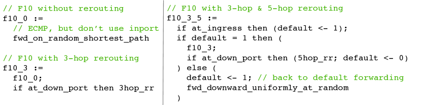
Figure 7. ProbNetKAT implementation of F10 in three refinement steps.

Now we will see how to encode several routing schemes using ProbNetKAT and analyze their behavior in each topology under various failure models.

Routing

F10 (Liu et al., 2013) provides a routing algorithm that combines the three routing and rerouting strategies we just discussed (ECMP, 3-hop rerouting, 5-hop rerouting) into a single scheme. We implemented it in three steps (see Figure 7). The first scheme, F10₀, implements an approach similar to ECMP: it chooses a port uniformly at random from the set of ports connected to minimum-length paths to the destination. We exclude the port at which the packet arrived from this set; this eliminates the possibility of forwarding loops when routing around failures.

Next, we improve the resilience of F10₀ by augmenting it with 3-hop rerouting if the next hop aggregation switch $A$ along the downward shortest path from a core switch $C$ fails. To illustrate, consider the blue path in Figure 6. We find a port on $C$ that connects to an aggregation switch $A^{\prime}$ of the opposite type than the failed aggregation switch, $A$, and forward the packet to $A^{\prime}$. If there are multiple such ports that have not failed, we choose one uniformly at random. Normal routing continues at $A^{\prime}$, and ECMP will know not to send the packet back to $C$. F10₃ implements this refinement.

Note that if the packet is still parked at port whose adjacent link is down after executing F10₃, it must be that all ports connecting to aggregation switches of the opposite type are down. In this case, we attempt 5-hop rerouting via an aggregation switch $A^{\prime\prime}$ of the same type as $A$. To illustrate, consider the red path in Figure 6. We begin by sending the packet to $A^{\prime\prime}$. To let $A^{\prime\prime}$ know that it should not send the packet back up as normally, we set a flag $\mathtt{default}$ to false in the packet, telling $A^{\prime\prime}$ to send the packet further down instead. From there, default routing continues. F10_3,5 implements this refinement.

$k$	$\widehat{\operatorname{M}}(\text{F10}\textsubscript{0},t,f_{k})$ $\equiv{\mathit{teleport}}$	$\widehat{\operatorname{M}}(\text{F10}\textsubscript{3},t,f_{k})$ $\equiv{\mathit{teleport}}$	$\widehat{\operatorname{M}}(\text{F10}\textsubscript{3,5},t,f_{k})$ $\equiv{\mathit{teleport}}$
0	✓	✓	✓
1	✗	✓	✓
2	✗	✓	✓
3	✗	✗	✓
4	✗	✗	✗
$\infty$	✗	✗	✗

Table 1. Evaluating $k$-resilience of F10.

$k$	$\mathtt{compare}$ $(\text{F10}\textsubscript{0},\text{F10}\textsubscript{3}\mathtt{)}$	$\mathtt{compare}$ $(\text{F10}\textsubscript{3},\text{F10}\textsubscript{3,5}\mathtt{)}$	$\mathtt{compare}$ $(\text{F10}\textsubscript{3,5},\mathit{teleport}\mathtt{)}$
0	$\equiv$	$\equiv$	$\equiv$
1	$<$	$\equiv$	$\equiv$
2	$<$	$\equiv$	$\equiv$
3	$<$	$<$	$\equiv$
4	$<$	$<$	$<$
$\infty$	$<$	$<$	$<$

Table 2. Comparing schemes under $k$ failures.

Failure and Network model

We define a family of failure models $f^{p}_{k}$ in the style of Section 2. Let $k\in\mathbb{N}\cup\{\infty\}$ denote a bound on the maximum number of link failures that may occur simultaneously, and assume that links otherwise fail independently with probability $0\leq p<1$ each. We omit $p$ when it is clear from context. For simplicity, to focus on the more complicated scenarios occurring on downward paths, we will model failures only for links connecting the aggregation and core layer.

Our network model works much like the one from Section 2. However, we model a single destination, switch 1, and we elide the final hop to the appropriate host connected to this switch.

$$\operatorname{M}(p,t)~{}\mathrel{\smash{\triangleq}}~{}in\mathbin{;}\mathsf{do}~{}(p\mathbin{;}t)~{}\mathsf{while}~{}(\neg\mathsf{sw}\kern 0.43057pt{=}\kern 0.43057pt1)$$

The ingress predicate $in$ is a disjunction of switch-and-port tests over all ingress locations. This first model is embedded into a refined model $\widehat{\operatorname{M}}(p,t,f)$ that integrates the failure model and declares all necessary local variables that track the healthiness of individual ports:

$$\widehat{\operatorname{M}}(p,t,f)~{}\mathrel{\smash{\triangleq}}~{}~{} \mathsf{var}~{}\mathsf{up_{1}}\kern 0.43057pt{\leftarrow}\kern 0.43057pt1~{}\mathsf{in}$$

$$\quad\dots$$

$$\mathsf{var}~{}\mathsf{up_{d}}\kern 0.43057pt{\leftarrow}\kern 0.43057pt1~{}\mathsf{in}$$

$$\operatorname{M}((f\mathbin{;}p),t)$$

Here $d$ denotes the maximum degree of all nodes in the FatTree and AB FatTree topologies from Figures 6 and 6, which we encode as programs $\mathit{fattree}$ and $\mathit{abfattree}$. much like in Section 2.2.

6.3. Checking invariants

We can gain confidence in the correctness of our implementation of F10 by verifying that it maintains certain key invariants. As an example, recall our implementation of F10_3,5: when we perform 5-hop rerouting, we use an extra bit ($\mathit{default}$) to notify the next hop aggregation switch to forward the packet downwards instead of performing default forwarding. The next hop follows this instruction and also sets $\mathit{default}$ back to $1$. By design, the packet can not be delivered to the destination with $\mathit{default}$ set to $0$.

To verify this property, we check the following equivalence:

$$\forall t,k:\ \ \widehat{\operatorname{M}}(\text{F10}\textsubscript{3,5},\mathit{t},f_{k})\ \equiv\ \widehat{\operatorname{M}}(\text{F10}\textsubscript{3,5},\mathit{t},f_{k})\mathbin{;}\mathit{default}\kern 0.43057pt{=}\kern 0.43057pt1$$

We executed the check using our implementation for $k\in\{0,1,2,3,4,\infty\}$ and $t\in\{\mathit{fattree},\mathit{abfattree}\}$. As discussed below, we actually failed to implement this feature correctly on our first attempt due to a subtle bug—we neglected to initialize the $\mathtt{default}$ flag to $1$ at the ingress.

6.4. F10 routing with FatTree

We previously saw that the structure of FatTree doesn’t allow 3-hop rerouting on failures because all subtrees are of the same type. This would mean that augmenting ECMP with 3-hop rerouting should have no effect, i.e. 3-hop rerouting should never kick in and act as a no-op. To verify this, we can check the following equivalence:

$$\forall k:\ \ \widehat{\operatorname{M}}(\text{F10}\textsubscript{0},\mathit{fattree},f_{k})\ \equiv\ \widehat{\operatorname{M}}(\text{F10}\textsubscript{3},\mathit{fattree},f_{k})$$

We have used our implementation to check that this equivalence indeed holds for $k\in\{0,1,2,3,4,\infty\}$.

6.5. Refinement

Recall that we implemented F10 in three stages. We started with a basic routing scheme (F10₀) based on ECMP that provides resilience on the upward path, but no rerouting capabilities on the downward paths. We then augmented this scheme by adding 3-hop rerouting to obtain F10₃, which can route around certain failures in the aggregation layer. Finally, we added 5-hop rerouting to address failure cases that 3-hop rerouting cannot handle, obtaining F10_3,5. Hence, we would expect the probability of packet delivery to increase with each refinement of our routing scheme. Additionally, we expect all schemes to deliver packets and drop packets with some probability under the unbounded failure model. These observations are summarized by the following ordering:

$$\mathsf{drop}\ <\ \widehat{\operatorname{M}}(\text{F10}\textsubscript{0},t,f_{\infty})\ <\ \widehat{\operatorname{M}}(\text{F10}\textsubscript{3},t,f_{\infty})\ <\ \widehat{\operatorname{M}}(\text{F10}\textsubscript{3,5},t,f_{\infty})\ <\ {\mathit{teleport}}$$

where $t=\mathit{abfattree}$ and $\mathit{teleport}\mathrel{\smash{\triangleq}}\mathsf{sw}\kern 0.43057pt{\leftarrow}\kern 0.43057pt1$. To our surprise, we were not able to verify this property initially, as our implementation indicated that the ordering

$$\widehat{\operatorname{M}}(\text{F10}\textsubscript{3},t,f_{\infty})\ <\ \widehat{\operatorname{M}}(\text{F10}\textsubscript{3,5},t,f_{\infty})$$

was violated. We then added a capability to our implementation to obtain counterexamples, and found that F10₃ performed better than F10_3,5 for packets $\pi$ with $\pi.\mathit{default}=0$. We were missing the first line in our implementation of F10_3,5 (cf., Figure 7) that initializes the $\mathit{default}$ bit to 1 at the ingress, causing packets to be dropped! After fixing the bug, we were able to confirm the expected ordering.

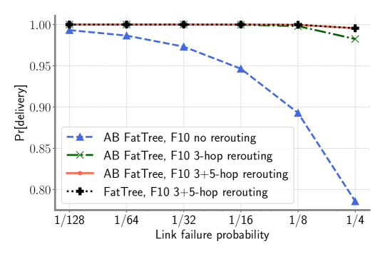
Figure 8. Probability of delivery vs. link-failure probability. ($k=\infty$).

6.6. k-resilience

We saw that there exists a strict ordering in terms of resilience for F10₀, F10₃ and F10_3,5 when an unbounded number of failures can happen. Another interesting way of measuring resilience is to count the minimum number of failures at which a scheme fails to guarantee 100% delivery. Using ProbNetKAT, we can measure this resilience by setting $k$ in $f_{k}$ to increasing values and checking equivalence with teleportation. Table 2 shows the results based on our decision procedure for the AB FatTree topology from  Figure 6.

The naive scheme, F10₀, which does not perform any rerouting, drops packets when a failure occurs on the downward path. Thus, it is 0-resilient. In the example topology, 3-hop rerouting has two possible ways to reroute for the given failure. Even if only one of the type B subtrees is reachable, F10₃ can still forward traffic. However, if both the type B subtrees are unreachable, then F10₃ will not be able to reroute traffic. Thus, F10₃ is 2-resilient. Similarly, F10_3,5 can route as long as any aggregation switch is reachable from the core switch. For F10_3,5 to fail the core switch would need to be disconnected from all four aggregation switches. Hence it is 3-resilient. In cases where schemes are not equivalent to $\mathit{teleport}$, we can characterize the relative robustness by computing the ordering, as shown in  Table 2.

6.7. Resilience under increasing failure rate

We can also do more quantitative analyses such as evaluating the effect of increase failure probability of links on the probability of packet delivery. Figure 8 shows this analysis in a failure model in which an unbounded number of failures can occur simultaneously. We find that F10₀’s delivery probability dips significantly as the failure probability increases because F10₀ is not resilient to failures. In contrast, both F10₃ and F10_3,5 continue to ensure high probability of delivery by rerouting around failures.

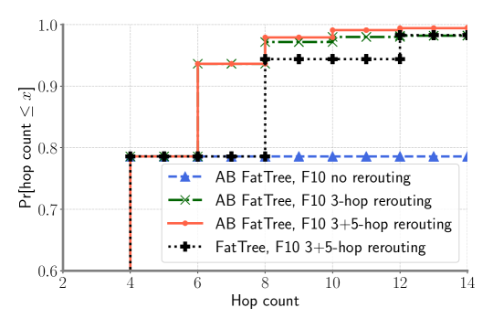
Figure 9. Increased latency due to resilience. ($k=\infty$, $p=\frac{1}{4}$)

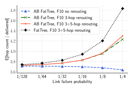
Figure 10. Expected hop-count conditioned on delivery. ($k=\infty$).

6.8. Cost of resilience

By augmenting naive routing schemes with rerouting mechanisms, we are able to achieve a higher degree of resilience. But this benefit comes at a cost. The detours taken to reroute traffic increase the latency (hop count) for packets. ProbNetKAT enables quantifying this increase in latency by augmenting our model with a counter that gets increased at every hop. Figure 9 shows the CDF of latency as the fraction of traffic delivered within a given hop count. On AB FatTree, we find that F10₀ delivers as much traffic as it can ($\approx$80%) within a hop count $\leq$ 4 because the maximum length of a shortest path from any edge switch to $s1$ is 4 and F10₀ does not use any longer paths. F10₃ and F10_3,5 deliver the same amount of traffic with hop count $\leq 4$. But, with 2 additional hops, they are able to deliver significantly more traffic because they perform 3-hop rerouting to handle certain failures. With 4 additional hops, F10_3,5’s throughput increases as 5-hop rerouting helps. We find that F10₃ also delivers more traffic with 8 hops—these are the cases when F10₃ performs 3-hop rerouting twice for a single packet as it encountered failure twice. Similarly, we see small increases in throughput for higher hop counts. We find that F10_3,5 improves resilience for FatTree too, but the impact on latency is significantly higher as FatTree does not support 3-hop rerouting.

6.9. Expected latency

Figure 10 shows the expected hop-count of paths taken by packets conditioned on their delivery. Both F10₃ and F10_3,5 deliver packets with high probability even at high failure probabilities, as we saw in Figure 8. However, a higher probability of link-failure implies that it becomes more likely for these schemes to invoke rerouting, which increases hop count. Hence, we see the increase in expected hop-count as failure probability increases. F10_3,5 uses 5-hop rerouting to achieve more resilience compared to F10₃, which performs only 3-hop rerouting, and this leads to slightly higher expected hop-count for F10_3,5. We see that the increase is more significant for FatTree in contrast to AB FatTree because FatTree only supports 5-hop rerouting.

As the failure probability increases, the probability of delivery for packets that are routed via the core layer decreases significantly for F10₀ (recall Figure 8). Thus, the distribution of delivered packets shifts towards those with direct 2-hop path via an aggregation switch (such as packets from $s2$ to $s1$), and hence the expected hop-count decreases slightly.

6.10. Discussion

As this case study of resilient routing in datacenters shows, the stochastic matrix representation of ProbNetKAT programs and accompanying decision procedure enable us to answer a wide variety of questions about probabilistic networks completely automatically. These new capabilities represent a signficant advance over current network verification tools, which are based on deterministic packet-forwarding models (Kazemian et al., 2012; Mai et al., 2011; Khurshid et al., 2012; Foster et al., 2015).

7. Deciding Full ProbNetKAT: Obstacles and Challenges

As we have just seen, history-free ProbNetKAT can describe sophisticated network routing schemes under various failure models, and program equivalence for the language is decidable. However, it is less expressive than the original ProbNetKAT language, which includes an additional primitive $\mathsf{dup}$. Intuitively, this command duplicates a packet $\pi\in\mathsf{Pk}$ and outputs the word $\pi\pi\in\mathsf{H}$, where $\mathsf{H}=\mathsf{Pk}^{*}$ is the set of non-empty, finite sequences of packets. An element of $\mathsf{H}$ is called a packet history, representing a log of previous packet states. ProbNetKAT policies may only modify the first (head) packet of each history; $\mathsf{dup}$ fixes the current head packet into the log by copying it. In this way, ProbNetKAT policies can compute distributions over the paths used to forward packets, instead of just over the final output packets.

However, with $\mathsf{dup}$, the semantics of ProbNetKAT becomes significantly more complex. Policies $p$ now transform sets of packet histories $a\in\smash{2^{\mathsf{H}}}$ to distributions $\llbracket p\rrbracket(a)\in\operatorname{\mathcal{D}}(\smash{2^{\mathsf{H}}})$. Since $\smash{2^{\mathsf{H}}}$ is uncountable, these distributions are no longer guaranteed to be discrete, and formalizing the semantics requires full-blown measure theory (see prior work for details (Smolka et al., 2017)).

Deciding program equivalence also becomes more challenging. Without $\mathsf{dup}$, policies operate on sets of packets $\smash{2^{\mathsf{Pk}}}$; crucially, this is a finite set and we can represent each set with a single state in a finite Markov chain. With $\mathsf{dup}$, policies operate on sets of packet histories $\smash{2^{\mathsf{H}}}$. Since this set is not finite—in fact, it is not even countable—encoding each packet history as a state would give a Markov chain with infinitely many states. Procedures for deciding equivalence are not known for such systems.

While in principle there could be a more compact representation of general ProbNetKAT policies as finite Markov chains or other models where equivalence is decidable, (e.g., weighted or probabilistic automata (Droste et al., 2009) or quantitative variants of regular expressions (Alur et al., 2016)), we suspect that deciding equivalence in the presence of $\mathsf{dup}$ is intractable. As evidence in support of this conjecture, we show that ProbNetKAT policies can simulate the following kind of probabilistic automata. This model appears to be new, and may be of independent interest.

Definition 7.1.

Let $A$ be a finite alphabet. A 2-generative probabilistic automata is defined by a tuple $(S,s_{0},\rho,\tau)$ where $S$ is a finite set of states; $s_{0}\in S$ is the initial state; $\rho:S\to(A\cup\{\_\})^{2}$ maps each state to a pair of letters $(u,v)$, where either $u$ or $v$ may be a special blank character $\_$; and the transition function $\tau:S\to\operatorname{\mathcal{D}}(S)$ gives the probability of transitioning from one state to another.

The semantics of an automaton can be defined as a probability measure on the space $A^{\infty}\times A^{\infty}$, where $A^{\infty}$ is the set of finite and (countably) infinite words over the alphabet $A$. Roughly, these measures are fully determined by the probabilities of producing any two finite prefixes of words $(w,w^{\prime})\in A^{*}\times A^{*}$.

Presenting the formal semantics would require more concepts from measure theory and take us far afield, but the basic idea is simple to describe. An infinite trace of a 2-generative automata over states $s_{0},s_{1},s_{2},\dots$ gives a sequence of pairs of (possibly blank) letters:

$$\rho(s_{0}),\rho(s_{1}),\rho(s_{2})\dots$$

By concatenating these pairs together and dropping all blank characters, a trace induces two (finite or infinite) words over the alphabet $A$. For example, the sequence,

$$(a_{0},\_),(a_{1},\_),(\_,a_{2}),\dots$$

gives the words $a_{0}a_{1}\dots$ and $a_{2}\dots$. Since the traces are generated by the probabilistic transition function $\tau$, each automaton gives rise to a probability measure over pairs of words.

While we have no formal proof of hardness, deciding equivalence between these automata appears highly challenging. In the special case where only one word is generated (say, when the second component produced is always blank), these automata are equivalent to standard automata with $\varepsilon$-transitions (e.g., see (Mohri, 2000)). In the standard setting, non-productive steps can be eliminated and the automata can be modeled as a finite state Markov chain, where equivalence is decidable. In our setting, however, steps producing blank letters in one component may produce non-blank letters in the other. As a result, it is not entirely clear how to eliminate these steps and encode our automata as a Markov chain.

Returning to ProbNetKAT, 2-generative automata can be encoded as policies with $\mathsf{dup}$. We sketch the idea here, deferring further details to Appendix B. Suppose we are given an automaton $(S,s_{0},\rho,\tau)$. We build a ProbNetKAT policy over packets with two fields, $\mathsf{st}$ and $\mathsf{id}$. The first field $\mathsf{st}$ ranges over the states $S$ and the alphabet $A$, while the second field $\mathsf{id}$ is either $1$ or $2$; we suppose the input set has exactly two packets labeled with $\mathsf{id}=1$ and $\mathsf{id}=2$. In a set of packet history, the two active packets have the same value for $\mathsf{st}\in S$—this represents the current state in the automata. Past packets in the history have $\mathsf{st}\in A$, representing the words produced so far; the first and second components of the output are tracked by the histories with $\mathsf{id}=1$ and $\mathsf{id}=2$. We can encode the transition function $\tau$ as a probabilistic choice in ProbNetKAT, updating the current state $\mathsf{st}$ of all packets, and recording non-blank letters produced by $\rho$ in the two components by applying $\mathsf{dup}$ on packets with the corresponding value of $\mathsf{id}$.

Intuitively, a set of packet histories generated by the resulting ProbNetKAT term describes a pair of words generated by the original automaton. With a bit more bookkeeping (see Appendix B), we can show that two 2-generative automata are equivalent if and only if their encoded ProbNetKAT policies are equivalent. Thus, deciding equivalence for ProbNetKAT with $\mathsf{dup}$ is harder than deciding equivalence for 2-generative automata. Showing hardness for the full framework is a fascinating open question. At the same time, deciding equivalence between $2$-generative automata appears to require substantially new ideas; these insights could shed light on how to decide equivalence for the full ProbNetKAT language.

8. Related Work

A key ingredient that underpins the results in this paper is the idea of representing the semantics of iteration using absorbing Markov chains, and exploiting their properties to directly compute limiting distributions on them.

Markov chains have been used by several authors to represent and to analyze probabilistic programs. An early example of using Markov chains for modeling probabilistic programs is the seminal paper by Sharir, Pnueli, and Hart (Sharir et al., 1984). They present a general method for proving properties of probabilistic programs. In their work, a probabilistic program is modeled by a Markov chain and an assertion on the output distribution is extended to an invariant assertion on all intermediate distributions (providing a probabilistic generalization of Floyd’s inductive assertion method). Their approach can assign semantics to infinite Markov chains for infinite processes, using stationary distributions of absorbing Markov chains in a similar way to the one used in this paper. Note however that the state space used in this and other work is not like ProbNetKAT’s current and accumulator sets ($2^{Pk}\times 2^{Pk}$), but is instead is the Cartesian product of variable assignments and program location. In this sense, the absorbing states occur for program termination, rather than for accumulation as in ProbNetKAT. Although packet modification is clearly related to variable assignment, accumulation does not clearly relate to program location.

Readers familiar with prior work on probabilistic automata might wonder if we could directly apply known results on (un)decidability of probabilistic rational languages. This is not the case—probabilistic automata accept distributions over words, while ProbNetKAT programs encode distributions over languages. Similarly, probabilistic programming languages, which have gained popularity in the last decade motivated by applications in machine learning, focus largely on Bayesian inference. They typically come equipped with a primitive for probabilistic conditioning and often have a semantics based on sampling. Working with ProbNetKAT has a substantially different style, in that the focus is on on specification and verification rather than inference.

Di Pierro, Hankin, and Wiklicky have used probabilistic abstract interpretation (PAI) to statically analyze probabilistic $\lambda$-calculus (Di Pierro et al., 2005). They introduce a linear operator semantics (LOS) and demonstrate a strictness analysis, which can be used in deterministic settings to replace lazy with eager evaluation without loss. Their work was later extended to a language called $pWhile$, using a store plus program location state-space similar to (Sharir et al., 1984). The language $pWhile$ is a basic imperative language comprising while-do and if-then-else constructs, but augmented with random choice between program blocks with a rational probability, and limited to a finite of number of finitely-ranged variables (in our case, packet fields). The authors explicitly limit integers to finite sets for analysis purposes to maintain finiteness, arguing that real programs will have fixed memory limitations. In contrast to our work, they do not deal with infinite limiting behavior beyond stepwise iteration, and do not guarantee convergence. Probabilistic abstract interpretation is a new but growing field of research (Wang et al., 2018).

Olejnik, Wicklicky, and Cheraghchi provided a probabilistic compiler $pwc$ for a variation of $pWhile$ (Olejnik et al., 2016), implemented in OCaml, together with a testing framework. The $pwc$ compiler has optimizations involving, for instance, the Kronecker product to help control matrix size, and a Julia backend. Their optimizations based on the Kronecker product might also be applied in, for instance, the generation of $\mathcal{S}\llbracket p\rrbracket$ from $\mathcal{B}\llbracket p\rrbracket$, but we have not pursued this direction as of yet.

There is a plenty of prior work on finding explicit distributions of probabilistic programs. Gordon, Henzinger, Nori, and Rajamani surveyed the state of the art with regard to probabilistic inference (Gordon et al., 2014). They show how stationary distributions on Markov chains can be used for the semantics of infinite probabilistic processes, and how they converge under certain conditions. Similar to our approach, they use absorbing strongly-connected-components to represent termination.

Markov chains are used in many probabilistic model checkers, of which PRISM (Kwiatkowska et al., 2011) is a prime example. PRISM supports analysis of discrete-time Markov chains, continuous-time Markov chains, and Markov decision processes. The models are checked against specifications written in temporal logics like PCTL and CSL. PRISM is written in Java and C++ and provides three model checking engines: a symbolic one with (multi-terminal) binary decision diagrams ((MT)BDDs), a sparse matrix one, and a hybrid. The use of PRISM to analyse ProbNetKAT programs is an interesting research avenue and we intend to explore it in the future.

9. Conclusion

This paper settles the decidability of program equivalence for history-free ProbNetKAT. The key technical challenge is overcome by modeling the iteration operator as an absorbing Markov chain, which makes it possible to compute a closed-form solution for its semantics. The resulting tool is useful for reasoning about a host of other program properties unrelated to equivalence. Natural directions for future work include investigating equivalence for full ProbNetKAT, developing an optimized implementation, and exploring new applications to networks and beyond.

Appendix A Omitted Proofs

Lemma A.1.

Let $A$ be a finite boolean combination of basic open sets, i.e. sets of the form $B_{a}=\{a\}\uparrow$ for $a\in\raisebox{1.0pt}{$\wp$\kern-0.7pt}_{\omega}(\mathsf{H})$, and let $\llparenthesis-\rrparenthesis$ denote the semantics from (Smolka et al., 2017). Then for all programs $p$ and inputs $a\in\smash{2^{\mathsf{H}}}$,

$$\llparenthesis p^{*}\rrparenthesis(a)(A)=\lim_{n\to\infty}\llparenthesis p^{(n)}\rrparenthesis(a)(A)$$

Proof 13.

Using topological arguments, the claim follows directly from previous results: $A$ is a Cantor-clopen set by (Smolka et al., 2017) (i.e., both $A$ and $\overline{A}$ are Cantor-open), so its indicator function $\mathbf{1}_{A}$ is Cantor-continuous. But $\mu_{n}\mathrel{\smash{\triangleq}}\llparenthesis p^{(n)}\rrparenthesis(a)$ converges weakly to $\mu\mathrel{\smash{\triangleq}}\llparenthesis p^{*}\rrparenthesis(a)$ in the Cantor topology (Theorem 4 in (Foster et al., 2016)), so

$$\lim_{n\to\infty}\llparenthesis p^{(n)}\rrparenthesis(a)(A)=\lim_{n\to\infty}\int\mathbf{1}_{A}d\mu_{n}=\int\mathbf{1}_{A}d\mu=\llparenthesis p^{*}\rrparenthesis(a)(A)$$

(To see why $A$ and $\overline{A}$ are open in the Cantor topology, note that they can be written in disjunctive normal form over atoms $B_{\{h\}}$.)

Proof of Proposition 3.1.

We only need to show that for $\mathsf{dup}$-free programs $p$ and history-free inputs $a\in\smash{2^{\mathsf{Pk}}}$, $\llparenthesis p\rrparenthesis(a)$ is a distribution on packets (where we identify packets and singleton histories). We proceed by structural induction on $p$. All cases are straightforward except perhaps the case of $p^{*}$. For this case, by the induction hypothesis, all $\llbracket p^{(n)}\rrbracket(a)$ are discrete probability distributions on packet sets, therefore vanish outside $\smash{2^{\mathsf{Pk}}}$. By Lemma A.1, this is also true of the limit $\llbracket p^{*}\rrbracket(a)$, as its value on $\smash{2^{\mathsf{Pk}}}$ must be 1, therefore it is also a discrete distribution on packet sets. ∎

Proof of Lemma 3.3.

This follows directly from Lemma A.1 and Proposition 3.1 by noticing that any set $A\subseteq\smash{2^{\mathsf{Pk}}}$ is a finite boolean combination of basic open sets. ∎

Lemma A.2.

The matrix $X=I-Q$ in Equation (3) of §5.1 is invertible.

Proof 14.

Let $S$ be a finite set of states, $|S|=n$, $M$ an $S\times S$ substochastic matrix ($M_{st}\geq 0$, $M\mathbf{1}\leq\mathbf{1}$). A state $s$ is defective if $(M\mathbf{1})_{s}<1$. We say $M$ is stochastic if $M\mathbf{1}=\mathbf{1}$, irreducible if $(\sum_{i=0}^{n-1}M^{i})_{st}>0$ (that is, the support graph of $M$ is strongly connected), and aperiodic if all entries of some power of $M$ are strictly positive.

We show that if $M$ is substochastic such that every state can reach a defective state via a path in the support graph, then the spectral radius of $M$ is strictly less than $1$. Intuitively, all weight in the system eventually drains out at the defective states.

Let $e_{s}$, $s\in S$, be the standard basis vectors. As a distribution, $e_{s}^{T}$ is the unit point mass on $s$. For $A\subseteq S$, let $e_{A}=\sum_{s\in A}e_{s}$. The $L_{1}$-norm of a substochastic vector is its total weight as a distribution. Multiplying on the right by $M$ never increases total weight, but will strictly decrease it if there is nonzero weight on a defective state. Since every state can reach a defective state, this must happen after $n$ steps, thus $\|e_{s}^{T}M^{n}\|_{1}<1$. Let $c=\max_{s}\|e_{s}^{T}M^{n}\|_{1}<1$. For any $y=\sum_{s}a_{s}e_{s}$,

$$\|y^{T}M^{n}\|_{1} =\|(\sum_{s}a_{s}e_{s})^{T}M^{n}\|_{1}$$

$$\leq\sum_{s}|a_{s}|\cdot\|e_{s}^{T}M^{n}\|_{1}\leq\sum_{s}|a_{s}|\cdot c=c\cdot\|y^{T}\|_{1}.$$

Then $M^{n}$ is contractive in the $L_{1}$ norm, so $|\lambda|<1$ for all eigenvalues $\lambda$. Thus $I-M$ is invertible because $1$ is not an eigenvalue of $M$.

Appendix B Encoding 2-Generative Automata in Full ProbNetKAT

To keep notation light, we describe our encoding in the special case where the alphabet $A=\{x,y\}$, there are four states $S=\{s_{1},s_{2},s_{3},s_{4}\}$, the initial state is $s_{1}$, and the output function $\rho$ is

$$\rho(s_{1})=(x,\_)\qquad\rho(s_{2})=(y,\_)\qquad\rho(s_{3})=(\_,x)\qquad\rho(s_{4})=(\_,y).$$

Encoding general automata is not much more complicated. Let $\tau:S\to\operatorname{\mathcal{D}}(S)$ be a given transition function; we write $p_{i,j}$ for $\tau(s_{i})(s_{j})$. We will build a ProbNetKAT policy simulating this automaton. Packets have two fields, $\mathsf{st}$ and $\mathsf{id}$, where $\mathsf{st}$ ranges over $S\cup A\cup\{\bullet\}$ and $\mathsf{id}$ ranges over $\{1,2\}$. Define:

$$p\mathrel{\smash{\triangleq}}\mathsf{st}\kern 0.43057pt{=}\kern 0.43057pts_{1}\mathbin{;}\mathsf{loop}^{*}\mathbin{;}\mathsf{st}\kern 0.43057pt{\leftarrow}\kern 0.43057pt\bullet$$

The initialization keeps packets that start in the initial state, while the final command marks histories that have exited the loop by setting $\mathsf{st}$ to be special letter $\bullet$.

The main program $\mathsf{loop}$ first branches on the current state $\mathsf{st}$:

$$\mathsf{loop}\mathrel{\smash{\triangleq}}\text{case }\begin{cases}\mathsf{st}\kern 0.43057pt{=}\kern 0.43057pts_{1}:\mathsf{state}1\\ \mathsf{st}\kern 0.43057pt{=}\kern 0.43057pts_{2}:\mathsf{state}2\\ \mathsf{st}\kern 0.43057pt{=}\kern 0.43057pts_{3}:\mathsf{state}3\\ \mathsf{st}\kern 0.43057pt{=}\kern 0.43057pts_{4}:\mathsf{state}4\end{cases}$$

Then, the policy simulates the behavior from each state. For instance:

$$\mathsf{state1}\mathrel{\smash{\triangleq}}\bigoplus\begin{cases}(\mathsf{if}~{}\mathsf{id}\kern 0.43057pt{=}\kern 0.43057pt1~{}\mathsf{then}~{}\mathsf{st}\kern 0.43057pt{\leftarrow}\kern 0.43057ptx\mathbin{;}\mathsf{dup}~{}\mathsf{else}~{}\mathsf{skip})\mathbin{;}\mathsf{st}\kern 0.43057pt{\leftarrow}\kern 0.43057pts_{1}\mathbin{@}p_{1,1},\\ (\mathsf{if}~{}\mathsf{id}\kern 0.43057pt{=}\kern 0.43057pt1~{}\mathsf{then}~{}\mathsf{st}\kern 0.43057pt{\leftarrow}\kern 0.43057pty\mathbin{;}\mathsf{dup}~{}\mathsf{else}~{}\mathsf{skip})\mathbin{;}\mathsf{st}\kern 0.43057pt{\leftarrow}\kern 0.43057pts_{2}\mathbin{@}p_{1,2},\\ (\mathsf{if}~{}\mathsf{id}\kern 0.43057pt{=}\kern 0.43057pt2~{}\mathsf{then}~{}\mathsf{st}\kern 0.43057pt{\leftarrow}\kern 0.43057ptx\mathbin{;}\mathsf{dup}~{}\mathsf{else}~{}\mathsf{skip})\mathbin{;}\mathsf{st}\kern 0.43057pt{\leftarrow}\kern 0.43057pts_{3}\mathbin{@}p_{1,3},\\ (\mathsf{if}~{}\mathsf{id}\kern 0.43057pt{=}\kern 0.43057pt2~{}\mathsf{then}~{}\mathsf{st}\kern 0.43057pt{\leftarrow}\kern 0.43057pty\mathbin{;}\mathsf{dup}~{}\mathsf{else}~{}\mathsf{skip})\mathbin{;}\mathsf{st}\kern 0.43057pt{\leftarrow}\kern 0.43057pts_{4}\mathbin{@}p_{1,4}\end{cases}$$

The policies $\mathsf{state2},\mathsf{state3},\mathsf{state4}$ are defined similarly.

Now, suppose we are given two 2-generative automata $W,W^{\prime}$ that differ only in their transition functions. For simplicity, we will further assume that both systems have strictly positive probability of generating a letter in either component in finitely many steps from any state. Suppose they generate distributions $\mu,\mu^{\prime}$ respectively over pairs of infinite words $A^{\omega}\times A^{\omega}$. Now, consider the encoded ProbNetKAT policies $p,p^{\prime}$. We argue that $\llbracket p\rrbracket=\llbracket q\rrbracket$ if and only if $\mu=\mu^{\prime}$.

First, it can be shown that $\llbracket p\rrbracket=\llbracket p^{\prime}\rrbracket$ if and only if $\llbracket p\rrbracket(e)=\llbracket p^{\prime}\rrbracket(e)$, where

$$e\mathrel{\smash{\triangleq}}\{\pi\pi\mid\pi\in\mathsf{Pk}\}.$$

Let $\nu=\llbracket p\rrbracket(e)$ and $\nu^{\prime}=\llbracket p^{\prime}\rrbracket(e)$. The key connection between the automata and the encoded policies is the following equality:

(7) $$\mu(S_{u,v})=\nu(T_{u,v})$$

for every pair of finite prefixes $u,v\in A^{*}$. In the automata distribution on the left, $S_{u,v}\subseteq A^{\omega}\times A^{\omega}$ consists of all pairs of infinite strings where $u$ is a prefix of the first component and $v$ is a prefix of the second component. In the ProbNetKAT distribution on the right, we first encode $u$ and $v$ as packet histories. For $i\in\{1,2\}$ representing the component and $w\in A^{*}$ a finite word, define the history

$$\mathit{h}_{i}(w)\in\mathsf{H}\mathrel{\smash{\triangleq}}(\mathsf{st}=\bullet,\mathsf{id}=i),(\mathsf{st}=w[|w|],\mathsf{id}=i),\dots,(\mathsf{st}=w[1],\mathsf{id}=i),(\mathsf{st}=s_{1},\mathsf{id}=i).$$

The letters of the word $w$ are encoded in reverse order because by convention, the head/newest packet is written towards the left-most end of a packet history, while the oldest packet is written towards the right-most end. For instance, the final letter $w[|w|]$ is the most recent (i.e., the latest) letter produced by the policy. Then, $T_{u,v}$ is the set of all history sets including $\mathit{h}_{1}(u)$ and $\mathit{h}_{2}(v)$:

$$T_{u,v}\mathrel{\smash{\triangleq}}\{a\in\smash{2^{\mathsf{H}}}\mid\mathit{h}_{1}(u)\in a,\mathit{h}_{2}(v)\in a\}.$$

Now $\llbracket p\rrbracket=\llbracket p^{\prime}\rrbracket$ implies $\mu=\mu^{\prime}$, since Equation 7 gives

$$\mu(S_{u,v})=\mu^{\prime}(S_{u,v}).$$

The reverse implication is a bit more delicate. Again by Equation 7, we have

$$\nu(T_{u,v})=\nu^{\prime}(T_{u,v}).$$

We need to extend this equality to all cones, defined by packet histories $\mathit{h}$:

$$B_{\mathit{h}}\mathrel{\smash{\triangleq}}\{a\in\smash{2^{\mathsf{H}}}\mid\mathit{h}\in a\}.$$

This follows by expressing $B_{\mathit{h}}$ as boolean combinations of $T_{u,v}$, and observing that the encoded policy produces only sets of encoded histories, i.e., where the most recent state $\mathsf{st}$ is set to $\bullet$ and the initial state $\mathsf{st}$ is set to $s_{1}$.

References

- (1)
- Al-Fares et al. (2008) Mohammad Al-Fares, Alexander Loukissas, and Amin Vahdat. 2008. A Scalable, Commodity Data Center Network Architecture. In ACM SIGCOMM Computer Communication Review, Vol. 38. ACM, 63–74.
- Alur et al. (2016) Rajeev Alur, Dana Fisman, and Mukund Raghothaman. 2016. Regular programming for quantitative properties of data streams. In ESOP 2016. 15–40.
- Anderson et al. (2014) Carolyn Jane Anderson, Nate Foster, Arjun Guha, Jean-Baptiste Jeannin, Dexter Kozen, Cole Schlesinger, and David Walker. 2014. NetKAT: Semantic Foundations for Networks. In POPL. 113–126.
- Bhatia et al. (2014) Manav Bhatia, Mach Chen, Sami Boutros, Marc Binderberger, and Jeffrey Haas. 2014. Bidirectional Forwarding Detection (BFD) on Link Aggregation Group (LAG) Interfaces. RFC 7130. (Feb. 2014). https://doi.org/10.17487/RFC7130
- Davis (2004) Timothy A. Davis. 2004. Algorithm 832: UMFPACK V4.3—an Unsymmetric-pattern Multifrontal Method. ACM Trans. Math. Softw. 30, 2 (June 2004), 196–199. https://doi.org/10.1145/992200.992206
- Di Pierro et al. (2005) Alessandra Di Pierro, Chris Hankin, and Herbert Wiklicky. 2005. Probabilistic -calculus and quantitative program analysis. Journal of Logic and Computation 15, 2 (2005), 159–179. https://doi.org/10.1093/logcom/exi008
- Droste et al. (2009) Manfred Droste, Werner Kuich, and Heiko Vogler. 2009. Handbook of Weighted Automata. Springer.
- Foster et al. (2016) Nate Foster, Dexter Kozen, Konstantinos Mamouras, Mark Reitblatt, and Alexandra Silva. 2016. Probabilistic NetKAT. In ESOP. 282–309. https://doi.org/10.1007/978-3-662-49498-1_12
- Foster et al. (2015) Nate Foster, Dexter Kozen, Matthew Milano, Alexandra Silva, and Laure Thompson. 2015. A Coalgebraic Decision Procedure for NetKAT. In POPL. ACM, 343–355.
- Gill et al. (2011) Phillipa Gill, Navendu Jain, and Nachiappan Nagappan. 2011. Understanding Network Failures in Data Centers: Measurement, Analysis, and Implications. In ACM SIGCOMM. 350–361.
- Giry (1982) Michele Giry. 1982. A categorical approach to probability theory. In Categorical aspects of topology and analysis. Springer, 68–85. https://doi.org/10.1007/BFb0092872
- Gordon et al. (2014) Andrew D Gordon, Thomas A Henzinger, Aditya V Nori, and Sriram K Rajamani. 2014. Probabilistic programming. In Proceedings of the on Future of Software Engineering. ACM, 167–181. https://doi.org/10.1145/2593882.2593900
- Guo et al. (2009) Chuanxiong Guo, Guohan Lu, Dan Li, Haitao Wu, Xuan Zhang, Yunfeng Shi, Chen Tian, Yongguang Zhang, and Songwu Lu. 2009. BCube: A High Performance, Server-centric Network Architecture for Modular Data Centers. ACM SIGCOMM Computer Communication Review 39, 4 (2009), 63–74.
- Guo et al. (2008) Chuanxiong Guo, Haitao Wu, Kun Tan, Lei Shi, Yongguang Zhang, and Songwu Lu. 2008. Dcell: A Scalable and Fault-Tolerant Network Structure for Data Centers. In ACM SIGCOMM Computer Communication Review, Vol. 38. ACM, 75–86.
- Kazemian et al. (2012) Peyman Kazemian, George Varghese, and Nick McKeown. 2012. Header Space Analysis: Static Checking for Networks. In USENIX NSDI 2012. 113–126. https://www.usenix.org/conference/nsdi12/technical-sessions/presentation/kazemian
- Kemeny et al. (1960) John G Kemeny, James Laurie Snell, et al. 1960. Finite markov chains. Vol. 356. van Nostrand Princeton, NJ.
- Khurshid et al. (2012) Ahmed Khurshid, Wenxuan Zhou, Matthew Caesar, and Brighten Godfrey. 2012. Veriflow: Verifying Network-Wide Invariants in Real Time. In ACM SIGCOMM. 467–472.
- Kozen (1981) Dexter Kozen. 1981. Semantics of probabilistic programs. J. Comput. Syst. Sci. 22, 3 (1981), 328–350. https://doi.org/10.1016/0022-0000(81)90036-2
- Kozen (1997) Dexter Kozen. 1997. Kleene Algebra with Tests. ACM TOPLAS 19, 3 (May 1997), 427–443. https://doi.org/10.1145/256167.256195
- Kwiatkowska et al. (2011) M. Kwiatkowska, G. Norman, and D. Parker. 2011. PRISM 4.0: Verification of Probabilistic Real-time Systems. In Proc. 23rd International Conference on Computer Aided Verification (CAV’11) (LNCS), G. Gopalakrishnan and S. Qadeer (Eds.), Vol. 6806. Springer, 585–591. https://doi.org/10.1007/978-3-642-22110-1_47
- Liu et al. (2013) Vincent Liu, Daniel Halperin, Arvind Krishnamurthy, and Thomas E Anderson. 2013. F10: A Fault-Tolerant Engineered Network. In USENIX NSDI. 399–412.
- Mai et al. (2011) Haohui Mai, Ahmed Khurshid, Rachit Agarwal, Matthew Caesar, P. Brighten Godfrey, and Samuel Talmadge King. 2011. Debugging the Data Plane with Anteater. In ACM SIGCOMM. 290–301.
- Mohri (2000) Mehryar Mohri. 2000. Generic -removal algorithm for weighted automata. In CIAA 2000. Springer, 230–242.
- Niranjan Mysore et al. (2009) Radhika Niranjan Mysore, Andreas Pamboris, Nathan Farrington, Nelson Huang, Pardis Miri, Sivasankar Radhakrishnan, Vikram Subramanya, and Amin Vahdat. 2009. Portland: A Scalable Fault-Tolerant Layer 2 Data Center Network Fabric. In ACM SIGCOMM Computer Communication Review, Vol. 39. ACM, 39–50.
- Olejnik et al. (2016) Maciej Olejnik, Herbert Wiklicky, and Mahdi Cheraghchi. 2016. Probabilistic Programming and Discrete Time Markov Chains. (2016). http://www.imperial.ac.uk/media/imperial-college/faculty-of-engineering/computing/public/MaciejOlejnik.pdf
- Roy et al. (2015) Arjun Roy, Hongyi Zeng, Jasmeet Bagga, George Porter, and Alex C. Snoeren. 2015. Inside the Social Network’s (Datacenter) Network. In ACM SIGCOMM. 123–137.
- Saheb-Djahromi (1980) N. Saheb-Djahromi. 1980. CPOs of measures for nondeterminism. Theoretical Computer Science 12 (1980), 19–37. https://doi.org/10.1016/0304-3975(80)90003-1
- Sharir et al. (1984) Micha Sharir, Amir Pnueli, and Sergiu Hart. 1984. Verification of probabilistic programs. SIAM J. Comput. 13, 2 (1984), 292–314. https://doi.org/10.1137/0213021
- Singla et al. (2012) Ankit Singla, Chi-Yao Hong, Lucian Popa, and P Brighten Godfrey. 2012. Jellyfish: Networking Data Centers Randomly. In USENIX NSDI. 225–238.
- Smolka et al. (2015) Steffen Smolka, Spiros Eliopoulos, Nate Foster, and Arjun Guha. 2015. A Fast Compiler for NetKAT. In ICFP 2015. https://doi.org/10.1145/2784731.2784761
- Smolka et al. (2017) Steffen Smolka, Praveen Kumar, Nate Foster, Dexter Kozen, and Alexandra Silva. 2017. Cantor Meets Scott: Semantic Foundations for Probabilistic Networks. In POPL 2017. https://doi.org/10.1145/3009837.3009843
- Tarjan (1975) Robert Endre Tarjan. 1975. Efficiency of a Good But Not Linear Set Union Algorithm. J. ACM 22, 2 (1975), 215–225. https://doi.org/10.1145/321879.321884
- Valiant (1982) L. Valiant. 1982. A Scheme for Fast Parallel Communication. SIAM J. Comput. 11, 2 (1982), 350–361.
- Wang et al. (2018) Di Wang, Jan Hoffmann, and Thomas Reps. 2018. PMAF: An Algebraic Framework for Static Analysis of Probabilistic Programs. In POPL 2018. https://www.cs.cmu.edu/~janh/papers/WangHR17.pdf