Exact Analytic Solution for a Ballistic Orbiting Wind
Abstract
Much theoretical and observational work has been done on stellar winds within binary systems. We present a new solution for a ballistic wind launched from a source in a circular orbit. Our method emphasizes the curved streamlines in the corotating frame, where the flow is steady-state, allowing us to obtain an exact solution for the mass density at all pre-shock locations. Assuming an initially isotropic wind, fluid elements launched from the interior hemisphere of the wind will be the first to cross other streamlines, resulting in a spiral structure bounded by two shock surfaces. Streamlines from the outer wind hemisphere later intersect these shocks as well. An analytic solution is obtained for the geometry of the two shock surfaces. Although the inner and outer shock surfaces asymptotically trace Archimedean spirals, our tail solution suggests many crossings where the shocks overlap, beyond which the analytic solution cannot be continued. Our solution can be readily extended to an initially anisotropic wind.
1 Introduction
Virtually all stars have a wind, and a large fraction of stars are in binary or multiple systems (Duchêne & Kraus, 2013), where the orbital motion will influence the flow of the wind. The motion of the driving source results in a “reflex” perturbation somewhat similar to parallax, whereby the flow is altered due to the changing location and velocity of the source (Soker, 1994; Cantó et al., 1999; He, 2007; Raga et al., 2011).
Binarity has been invoked as the cause of a wealth of structures in planetary nebulae and their asymptotic giant branch (AGB) precursors (Morris, 1981; Livio, 1982; Soker, 1994; Mastrodemos & Morris, 1999). Dramatic examples include spiral nebulae such as AFGL 3068 (Mauron & Huggins, 2006; Morris et al., 2006) and CIT 6 (Kim et al., 2013). Detailed analyses have been presented to use the nebular morphology and kinematics to diagnose unresolved features of the drivers, both to infer binarity and binary separation, as well as to determine wind properties (Kim & Taam, 2012; Homan et al., 2015). The gravitational wake mechanism (Kim, 2011; Kim & Taam, 2012) can also produce a spiral pattern, but has a more flattened morphology, allowing one to in principle distinguish the presence of two separate, spiral morphologies. Additionally, the presence of two winds in a binary system leads to a collision region bounded by two shocks, which may develop mixing in the presence of a wealth of instabilities (Myasnikov & Zhekov, 1991; Monnier et al., 1999; Lamberts et al., 2012; Rauw & Nazé, 2016; Hendrix et al., 2016).
We present a new, exact solution to the problem of an initially isotropic wind launched ballistically from an orbiting point source in a circular orbit. In §2 we describe the streamlines and kinematics, in §3 we derive the density structure, and §4 discusses the shock criterion and the implications of this work.
2 Mathematical Formulation
We consider a wind launched from an orbiting star. Although the motion will clearly be time-dependent, a steady-state flow pattern should exist in the reference frame corotating with the star’s orbital motion about the center of mass, provided the orbit is circular and the wind launch conditions are unchanging in that frame. Let the star orbit a distance from the origin in the X-Y plane, at angular frequency and counterclockwise as viewed from above. In the inertial frame the star’s position and velocity as a function of time are
| (1) | |||||
| (2) |
Here and are the usual unit vectors along the and axes. The Cartesian coordinates in the inertial and corotating (primed) frames are related by and
| (3) |
Now consider a fluid element launched from the star’s location, taken as a point source. Neglecting gravitational, pressure, and other forces, the fluid element has unchanging velocity in the inertial frame, provided that streamlines do not cross. Our neglect of gravitational force on the ballistically moving fluid element is most valid for wide binaries, where the launch speed is assumed characteristic of the depth of the gravitational well of the launching source, and much faster than the escape speed from the binary system. By assuming wind launch impulsively from a point source at time , we can write a fluid trajectory equation
| (4) |
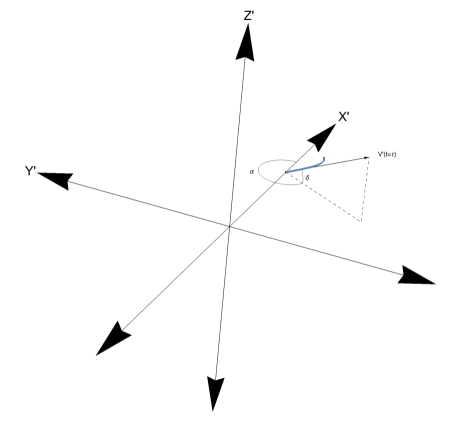
where The velocity of the fluid element in the inertial frame is the star’s velocity at the time of launch , plus the launch velocity in the comoving frame of the star for the appropriate launch direction. We define launch angles in the corotating frame, with being azimuthal angle counterclockwise relative to the axis, and is the latitude above the plane (see Figure 1).
The inverse transformation is used to obtain the unit vectors at the launch time:
| (5) |
If we take the initial launch of the wind in the corotating frame to be steady and isotropic, we have simply Here is a unit vector pointing radially away from the star and given in terms of the launch angles by
| (6) |
Using equations (1,2,4-6), the trajectory in the inertial frame in terms of the launch angles is given by:
| (7) |
where for brevity we have introduced . We nondimensionalize the equations by using length unit and time unit , so dimensionless position is with dimensionless components x, y, and z, and dimensionless velocity is We introduce the dimensionless parameter
| (8) |
as the ratio of orbital speed to wind launch speed. Using the inverse transformation from eqs.(5) (applied at time rather than ), and defining a time-like coordinate along the streamline as
| (9) |
we obtain the (dimensionless) trajectory in the corotating frame:
| (10) |
In spherical coordinates,
| (11) |
The (dimensional) velocity in the corotating frame can be obtained by taking the derivative of with respect to time . But since is constant as the fluid element moves, we can equivalently differentiate the dimensionless position with respect to s. This yields the primed, dimensionless velocity components
| (12) |
where . Equations (10) and (12) give a complete description of the wind kinematics in the corotating frame in parametric form. By taking the limit of no orbital motion, which corresponds to vanishing , we can see that these equations yield free streaming at the wind speed in the initial launch direction. We also require the magnitude of the velocity, whose square is given by
| (13) |
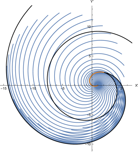
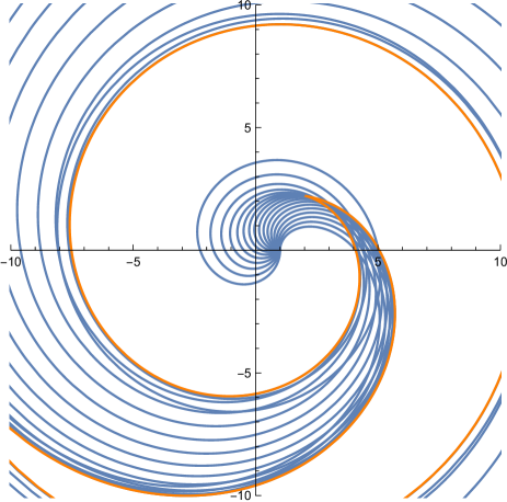
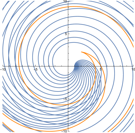
Figure 2 shows the streamline shape in the rotating frame for the value . Note the characteristic trailing spiral pattern. As will be described in §4, streamline crossing begins at the location of the inner and outer, solid black curves, depending on the -value of the streamline, and is confined to the region between them. Figure 3 shows the streamline shape in the rotating frame for four launch angles and three values of . The streamlines are nearly straight for small , and become increasingly distorted in a trailing spiral pattern at larger (and ) values. For sufficiently large values of (for any ), streamlines will eventually cross, indicating the formation of a shock.

3 Derivation of the fluid density
The behavior of the density as a function of position can be determined by solving the mass conservation equation in steady-state in the rotating frame. We introduce the density unit
| (14) |
where is the wind mass loss rate, so the dimensionless density is . Using , for regions where streamlines have not crossed, the mass conservation equation is
| (15) |
Our derivation will involve elements of tensor calculus because the most appropriate set of curvilinear coordinates will not result in an orthonormal basis. The reader unconcerned with the details may safely jump to equation (23), our result for the density.
We choose a set of coordinates , where the superscript is not an exponent but an index that takes values The natural (covariant) basis vectors with respect to these coordinates are given by
| (16) |
where the position vector is evaluated using equations (10). The first two basis vectors are
| (17) |
while the third is whose Cartesian components are given by eq.(12). Because the velocity vector is entirely in the direction of , the contravariant components of the velocity vector are , and .
The covariant metric tensor is symmetric, with elements given by
| (18) |
where , , and is given by equation (13). The determinant of the metric tensor is
| (19) |
This allows us to take a divergence using our coordinate system. For a vector the divergence is (Aris (1962), p.170)
| (20) |
If we apply this formula for divergence to the conservation of , according to equation (15), only the third term of the divergence is needed since the first two components vanish. We obtain upon integration
| (21) |
The function is determined by matching the above formula to the behavior close to the wind source where the flow is isotropic in the limit of small . Considering the mass density at a small radius centered on the source,
| (22) |
For this case we have the limit , implying . Equation (21) then gives the density as
| (23) |
On more intuitive grounds, mass conservation may be enforced in an integral sense by imagining a narrow streamtube, bounded along its length by streamlines. Mass may enter or leave the streamtube only at its ends: one located on a small spherical surface centered on the wind source, and the other at an arbitrary (but larger) constant value of s. Let the foot of the stream tube lie on a small sphere of radius , and have two sides of constant , and , and two sides of constant and . The area of the enclosed surface patch is . We generate a thin volume by including a thickness The amount of mass in this volume must equal that at the far end of the streamtube in a volume of matching , , and . The volume element at either end of the stream tube is described by the scalar triple product
| (24) |
The cross product defines a vector area element on a surface of constant , where
| (25) |
Dotting this with the velocity vector shows that the “volume factor” is identical to ,
| (26) |
Thus, in dimensional units, and using subscript ‘1’ at the inner point, with no subscript at the outer, which gives
| (27) |
Equation (27) is the dimensional form of our previous result, eq.(23).
4 Discussion
4.1 Streamline Crossing and Shocks
The expression for density contains a factor which for an isotropic wind from a stationary source (e.g., taking ) results in an inverse distance-squared dependence. But for a moving wind, this is more directly interpreted as an inverse square dependence on time since launch because for this scenario the distance from the source is not proportional to time. The additional factor in parentheses results in a density enhancement when , and a density deficit when . We will call these the inner (pointing toward the origin) and outer launch hemispheres, respectively. In fact, the density diverges when . Because we aren’t interested in the trivial divergence at the wind source, the vanishing of the factor in parentheses in equation (26) yields the condition along a given inner streamline (one for which ) that
| (28) |
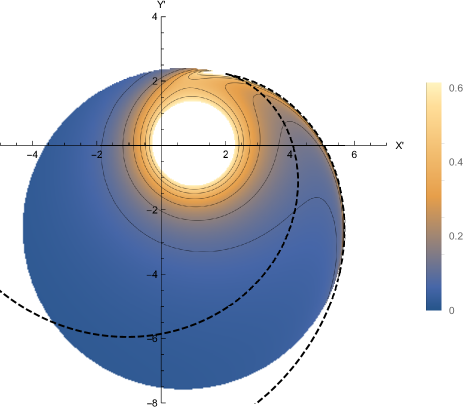
Figure 5 shows the outer branch of the predicted shock location for the more moderate222Soker (1994) estimates a range of p-values from 0.01-0.3 for wide binaries within planetary nebulae. value . For outer streamlines, defined by , the quantity never vanishes and the density remains finite. The surface where therefore represents a shock surface, and the formal streamline solutions cannot be applied to collisional fluids for . The condition for local streamline crossing can also be derived by assuming an arbitrary set of values for and demanding that two neighboring, but initially distinct fluid elements (the second having parameter values have the same position using equations (10). For brevity we will not present this lengthy calculation here, but note that it yields , reproducing our shock condition. Evidently exactly half of the stellar wind, the inner launch hemisphere, “self-shocks” in a local sense, while the other half doesn’t. The outer streamlines do, however, intersect the shock surface (see Figure(2)), so that eventually all streamlines except , , and will encounter a shock. The distinct trajectories of the inner and outer streamlines and their relationship to the inner and outer shocks are shown in Figures (6-7).
An examination of Figures(6-7) shows that two distinct types of streamline crossings occur. The “self-shocking” involves streamlines that cross their nearest neighbors, that is, those launched with only a differentially distinct angle. These overlaps are properly termed caustics, and can be located with our shock criterion. The second type of streamline crossing we shall term “non-local,” because initially widely-spaced streamlines may cross. This includes, but is not limited to, all the streamline crossings involving outer streamlines. Outer streamlines never have self-shocking, but by crossing the caustic boundaries they do cross inner streamlines. Additionally, within the caustic zone inner streamines cross an infinite number of other inner streamlines in a continuous fashion. We do not have a general solution for such non-local crossings, other than direct solution of equations (10), which proves to be very cumbersome. Nonetheless, Figures (6-7) show this behavior for the chosen value of p.
4.2 The Cusp
The innermost point on the shock surface is a needle-like cusp of vanishing opening angle in the orbital plane. The location of the point is found from equations (11,28) by solving for the launch angle resulting in minimal radius for the shock. The critical streamline that enters the cusp tangentially in the orbital plane has launch angle and value
| (29) | |||||
| (30) |
The location of the cusp is then found by using these values in the trajectory equation (11) as
| (31) |
We note that in the limit of small , equation (31) is consistent with the results of Raga et al. (2011) and Cantó et al. (1999), who assumed a purely radial wind of time-dependent speed, launched from the center of mass, obtaining in dimensional units . Our result generalizes this with an exact treatment of centrifugal and coriolis effects. Kim & Taam (2012) also give an empirical formula predicting a smaller standoff location based upon numerical simulations, although these simulations also incorporated gravitational perturbations. The discrepancy may be associated with the difficulty of determining the innermost location along the shock, because the convergence of streamlines prior to reaching the cusp results in a density enhancement which may have been interpreted as a cusp in their simulations. For , no cusp occurs, and there will be regions unreached by the flow due to a centrifugal barrier. In particular, note that the same streamline that intersects the cusp point also goes through the origin. For , the flow does not reach the origin, with implications for identical colliding winds: no stagnation point region would be possible. Because our neglect of gravitational forces was justified by application to wide binaries only (small ), we will not discuss the case .
4.3 The Shocked Region
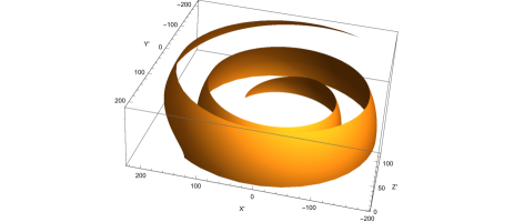
Our streamline analysis does not provide a description of the region between the two shock surfaces. However, an asymptotic, “tail” solution for the shock may be developed for the outer part of the shock spiral by noting that the azimuthal range is mapped to an infinite range of azimuthal angle in the outer region, so that most of the spiral corresponds to a small region of either or . Physically, this means most of the wind mass has reached the shock before many windings occur. Either limit yields by direct substitution into equation (28) and expansion to leading order. Substitution into equations (10) gives outer solution from , and inner solution from , as
| (32) | |||||
which yields radii for the two tails
| (33) |
Both tail solutions take the form of an Archimedean spiral where plays the role of azimuthal angle.
The radial spacing for a given curve is found by adding argument to , which gives
| (34) |
This radial step is a generalization of the expression given by Mauron & Huggins (2006); Raga et al. (2011) and agrees with both for vanishing . On the other hand, the radial spacing (fixed and ) between the two shock curves provides an estimate of the thickness of the shell of shocked gas. When evaluated for small , this radial thickness is , and using , the fractional thickness is Because the radial step for the inner shock is smaller than that for the outer shock, and these steps are approximately constant, the mis-match implies that eventually the outer shock for, say, n orbits, should cross the inner shock for n+1 orbits, resulting in a pinching-off of all unshocked streamlines. The intersection of two shocks may produce filamentary or spoke-like features, although for large enough intersection angle a Mach stem could result (e.g.Hartigan et al. (2016)). Given the complex spiral geometry, we cannot anticipate the details of such Mach structures here, and leave them for further study that could be done with 3-d hydrodynamics simulations.
4.4 Summary
We have considered the flow structure of an initially isotropic wind from a point source in a circular orbit. Assuming ballistic flow, the pre-shock particle trajectories are straight lines in the inertial frame of the center of mass, and trailing spirals in the frame rotating with the source. In the corotating frame, the flow is steady-state and trajectories are initially non-intersecting streamlines. By solving the mass conservation condition in a curvilinear coordinate system based upon these streamlines, we obtain an exact solution for the density structure. This density has a latitude and initial launch angle dependence. Interestingly, the usual dependence is modified as an inverse square dependence on time of flight, modified by a geometric factor.
The flow is separated into two behaviors. The inner launch hemisphere generates a converging flow so that streamlines eventually intersect with their neighbors, resulting in a shock. The outer hemisphere of launch has non-intersecting, diverging streamlines. However, outer streamlines do eventually run into the shock region. A local criterion for streamline crossing gives the region beyond which the description is incomplete. A full description of the post-shock flow as a spiral shell is beyond the scope of this study.
The generic nature of our model and the ubiquity of winds in widely-separated binaries imply that our solution should be applicable to modeling a wide variety of observed sources such as spiral nebulae of AGB stars, structures within planetary nebulae, and colliding winds in binary systems.
References
- Aris (1962) Aris, R. 1962, Vectors, Tensors, and the Basic Equations of Fluid Mechanics, Dover Publications, New York
- Cantó et al. (1999) Cantó, J., Raga, A. C., Koenigsberger, G., & Moreno, E. 1999, Wolf-Rayet Phenomena in Massive Stars and Starburst Galaxies, 193, 338
- Duchêne & Kraus (2013) Duchêne, G., & Kraus, A. 2013, ARA&A, 51, 269
- Hartigan et al. (2016) Hartigan, P., Foster, J., Frank, A., et al. 2016, ApJ, 823, 148
- He (2007) He, J. H. 2007, A&A, 467, 1081
- Hendrix et al. (2016) Hendrix, T., Keppens, R., van Marle, A. J., et al. 2016, MNRAS, 460, 3975
- Homan et al. (2015) Homan, W., Decin, L., de Koter, A., et al. 2015, A&A, 579, A118
- Kim (2011) Kim, H. 2011, ApJ, 739, 102
- Kim & Taam (2012) Kim, H., & Taam, R. E. 2012, ApJ, 744, 136
- Kim & Taam (2012) Kim, H., & Taam, R. E. 2012, ApJ, 759, 59
- Kim & Taam (2012) Kim, H., & Taam, R. E. 2012, ApJ, 759, L22
- Kim et al. (2013) Kim, H., Hsieh, I.-T., Liu, S.-Y., & Taam, R. E. 2013, ApJ, 776, 86
- Lamberts et al. (2012) Lamberts, A., Dubus, G., Lesur, G., & Fromang, S. 2012, A&A, 546, A60
- Livio (1982) Livio, M. 1982, A&A, 105, 37
- Mastrodemos & Morris (1999) Mastrodemos, N., & Morris, M. 1999, ApJ, 523, 357
- Mauron & Huggins (2006) Mauron, N., & Huggins, P. J. 2006, A&A, 452, 257
- Monnier et al. (1999) Monnier, J. D., Tuthill, P. G., & Danchi, W. C. 1999, ApJ, 525, L97
- Morris (1981) Morris, M. 1981, ApJ, 249, 572
- Morris et al. (2006) Morris, M., Sahai, R., Matthews, K., et al. 2006, Planetary Nebulae in our Galaxy and Beyond, 234, 469
- Myasnikov & Zhekov (1991) Myasnikov, A. V., & Zhekov, S. A. 1991, Ap&SS, 184, 287
- Raga et al. (2011) Raga, A.C., Cantó, J., Esquivel, A., Huggins, P.J. & Mauron, N. 2011, Aymmetric Planetary Nebulae V, Ed. Zijlstra, A.A., Lykou, F., McDonald, I. & Lagadec, E. 185
- Rauw & Nazé (2016) Rauw, G., & Nazé, Y. 2016, Advances in Space Research, 58, 761
- Soker (1994) Soker, N. 1994, MNRAS, 270, 774