Spectral features in the cosmic ray fluxes

Abstract

The cosmic ray energy distributions contain spectral features, that is narrow energy regions where the slope of the spectrum changes rapidly. The identification and study of these features is of great importance to understand the astrophysical mechanisms of acceleration and propagation that form the spectra. In first approximation a spectral feature in often described as a discontinuous change in slope, however very valuable information is also contained in its width, that is the length of the interval in logarithm of energy where the change in spectral index develops. In this work we discuss the best way to define and parametrize the width a spectral feature, and for illustration discuss some of the most prominent known structures.

1 Introduction

The spectra of cosmic rays (CR) extend to a very broad energy range with a smooth shape that, for energy $E\gtrsim 30$ GeV, is usually described as an ensemble of adjacent energy intervals, where the energy distribution is a simple power law ($\phi(E)\simeq K\;E^{-\alpha}$), separated by “spectral features”, that is narrow regions where the slope (or spectral index) of the flux undergoes a rapid change. The features can be softenings or hardenings of the spectrum, and appear as “knee–like” or “ankle–like” in the usual log–log graphic representation of the spectrum. Prominent and well known examples of features in the all particle spectrum are in fact the “Knee at $E\simeq 3$ PeV, and the “Ankle” at $E\simeq 4$ EeV.

The simple description outlined above is an approximation, because it is likely that the CR spectra are not, even in a limited range of energy, exactly of power law form, and the spectral indices are always slowly evolving with energy; however the identification and study of discrete spectral features can be considered as a natural and useful task.

It is obviously very desirable, and in fact ultimately necessary, to describe the CR spectral features in the framework of astrophysically motivated models, and in terms of parameters that have a real physical meaning, and in the literature there are several alternative models to interpret the observations. On the other hand, it is useful to have a purely phenomenological description of the shape of the spectral features, as an intermediate step that can be used as a guide in the construction of astrophysical models.

In first order approximation, a spectral feature can be described as infinitely narrow, with the spectral index that changes discontinuosly. In this limit a feature it is completely described by four parameters: $E_{b}$ the break energy, that gives its position, $\alpha_{1}$ and $\alpha_{2}$ the spectral slopes before and after the break, and the absolute normalization of the the flux.

It is obvious that the hypothesis of a discontinuous change in spectral slope is unphysical, and this suggests that a phenomenological description of a spectral feature should include at least one additional parameter. A simple and convenient parametrization of the spectral shape of the CR all particle spectrum in the region of the Knee has been introduced by Ter–Antonyan and Haroyan [1] and later used by Schatz [2]. This parametrization can be applied to the description of both softening and hardening spectral features and (with $E_{0}$ is an arbitrary reference energy) has the form:

$$\phi(E)=K_{0}\;\left(\frac{E}{E_{0}}\right)^{-\alpha_{1}}\;\left[1+\left(\frac{E}{E_{b}}\right)^{\frac{1}{w}}\right]^{-(\alpha_{2}-\alpha_{1})\,w}$$ (1)

that contains one additional parameter, the width $w>0$ (note that the authors of [1, 2] use the parameter $\varepsilon=1/w$). Some examples of the spectral shapes of this parametrization are shown in Fig. 1. For a more precise understanding of the “geometrical meaning” of $w$ it is useful to consider the energy dependence of the spectral index of a flux described by Eq. (1):

$$\alpha(E)\equiv-\frac{d\ln\phi}{d\ln E}=\overline{\alpha}+\frac{\Delta\alpha}{2}\;\tanh\left[\frac{\ln(E/E_{b})}{2w}\right]~{}.$$ (2)

In this equation $\overline{\alpha}=(\alpha_{2}+\alpha_{1})/2$ is the average of the two spectral indices before and after the break, and $\Delta\alpha=(\alpha_{2}-\alpha_{1})$ is the total change in spectral index across the break (some numerical examples are shown in Fig. 2). It is straightforward to see that $w$ gives the width of the energy range where the step in spectral index develops.

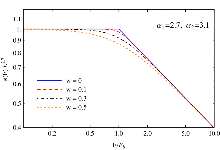
Figure 1: Example of a (softening) spectral feature described by the parametrization of Eq. (1). The spectral indices before and after the break are $\alpha_{1}=2.7$ and $\alpha_{2}=3.1$. The different curves are for $w=0$, 0.1, 0.3 and 0.5.

The limit $w\to 0$ of Eq. (2) is:

$$\lim_{w\to 0}\alpha(E)=\begin{cases}\overline{\alpha}-\frac{\Delta\alpha}{2}=\alpha_{1}&\text{for $E<E_{b}$}\\[7.11317pt] \overline{\alpha}+\frac{\Delta\alpha}{2}=\alpha_{2}&\text{for $E>E_{b}$}\end{cases}$$ (3)

and corresponds to a discontinuous jump of the spectral index. More in general, one has that the asymptotic values (for $E\to 0$ and $E\to\infty$) of the spectral index are $\alpha_{1}$ and $\alpha_{2}$, and at the break energy $E_{b}$ the spectral index takes the average value: $\alpha(E_{b})=\overline{\alpha}$. The jump $\Delta\alpha$ develops symmetrically in $\log E$, and the energies $E_{f_{\pm}}$ where the spectral index takes the values:

$$\alpha(E_{f_{\pm}})=\overline{\alpha}\pm\frac{\Delta\alpha}{2}\;f$$ (4)

(with $0\leq f<1$) are given by:

$$\log E_{f_{\pm}}=\log E_{b}\pm w\;\log\left[\frac{1+f}{1-f}\right]~{},$$ (5)

so that the two values $\log E_{f_{\pm}}$ are placed symmetrically with respect to $\log E_{b}$. The total range of $\log E$ (centered on $\log E_{b}$) where the spectral index varies by $\Delta\alpha/2$ is then:

$$(\Delta\log_{10}E)_{\Delta\alpha/2}=(\log_{10}9)\;w\simeq 0.954\;w~{}.$$ (6)

This allows to attribute a simple and easy to remember physical meaning to $w$. The value $w\simeq 1$ corresponds to a spectral feature that develops in approximately a decade of energy, and a feature of width $w\simeq 0.1$ has an energy extension that is approximately a factor $\approx 10^{0.1}\simeq 1.25$.

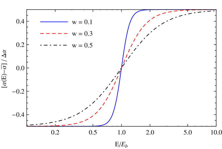
Figure 2: Energy dependence of the spectral index [see Eq. (2)]. The three curves correspond to three values of the width parameter ($w=0.1$, 0.3 and 0.5).

Recently the AMS02 collaboration has presented fits to the rigidity spectra of the proton an helium spectra using the parametrization (expressed here as a function of energy):

$$\phi(E)=K\;\left(\frac{E}{E_{0}}\right)^{-\alpha_{1}}\;\left[1+\left(\frac{E}{E_{b}}\right)^{-(\alpha_{2}-\alpha_{1})/s}\right]^{s}~{}.$$ (7)

Eqs. (1) and (7) are in fact different parametrizations of the same ensemble of curves. The parameter $s$ used in Eq. (7) is related to the width $w$ of Eq. (1) by:

$$s=\frac{w}{|\Delta\alpha|}~{},$$ (8)

and therefore Eqs. (1) and (7) are equivalent. However, we find that the use of the width parameter $w$ is is preferable because of its more transparent and intuitive physical meaning. In addition, when performing fits to data, the quantities in the pair {$s$, $\Delta\alpha$} are in general much more strongly correlated than the quantities in the pair {$w$, $\Delta\alpha$}.

As discussed above, the spectral index of a flux described by Eq. (1) or (7) is symmetric in $\log E$. It is potentially interesting to have a more flexible functional form to describe a spectral feature that allows for the possibility that the spectral index changes more rapidly before of after the break energy. A simple generalization of Eq. (1) that depends on one more parameter, can be obtained, keeping for $E_{b}$ the same definition, that is the energy where the spectral index takes the average value: $\alpha(E_{b})=(\alpha_{1}+\alpha_{2})/2$, and introducing two different widths to the left and right of the break energy. This results in the form:

$$\phi(E)=\begin{cases}K_{0}\;\left(\frac{E}{E_{0}}\right)^{-\alpha_{1}}\left[1+\left(\frac{E}{E_{b}}\right)^{\frac{1}{w_{L}}}\right]^{-\Delta\alpha\,w_{L}}&\text{for $E<E_{b}$}\\[8.5359pt] K_{0}\;2^{\Delta\alpha\,(w_{R}-w_{L})}\;\left(\frac{E}{E_{0}}\right)^{-\alpha_{1}}\;\left[1+\left(\frac{E}{E_{b}}\right)^{\frac{1}{w_{R}}}\right]^{-\Delta\alpha\,w_{R}}&\text{for $E>E_{b}$}~{},\end{cases}$$ (9)

so that the spectral index $\alpha(E)$ takes the form:

$$\alpha(E)=\begin{cases}\overline{\alpha}+\frac{\Delta\alpha}{2}\;\tanh\left[\frac{\ln(E/E_{b})}{2w_{L}}\right]&\text{for $E<E_{b}$}\\[7.11317pt] \overline{\alpha}+\frac{\Delta\alpha}{2}\;\tanh\left[\frac{\ln(E/E_{b})}{2w_{R}}\right]&\text{for $E>E_{b}$~{}}~{}.\end{cases}$$ (10)

For this parametrization the flux and its first derivative (i.e. the spectral index) are continuous, but the second derivative is discontinuous at the point $E=E_{b}$. Taking the derivative of the spectral index with respect to energy, one finds that the limits for $E\to E_{b}$ taken in the two directions are different:

$$\lim_{E\to(E_{b})^{\mp}}\frac{d\alpha(E)}{d\ln E}=\frac{\Delta\alpha}{4\,w_{L,R}}~{}.$$ (11)

This appear to be a tolerable flaw for the parametrization of Eq. (9).

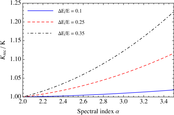
Figure 3: Effects of the detector finite resolution (assumed gaussian with constant $\Delta E/E$) on the normalization of a power law spectrum. The curves show the ratio $K_{\rm rec}/K$ plotted as a function of the spectral index $\alpha$ for three values of the resolution: $\Delta E/E=0.1$, 0.25, 0.35.

Having constructed this more general parametrization of a spectral feature, we have tested that for the level of precision of the existing data, the form that depends on a single width is in fact adequate to describe all known structures (see discussion in the following).

2 Detector resolution

The shape of an observed spectral feature is distorted by the detector resolution. To illustrate these instrumental effects one can consider a simple example where the energy of the events is reconstructed with gaussian errors and a constant $\Delta E/E$. With this assumption a spectrum that is an unbroken power law $\phi(E)=K\,E^{-\alpha}$ results (in the absence of an unfolding) in a reconstructed spectrum that is a power law with the same exponent: $\phi_{\rm rec}(E_{\rm rec})=K_{\rm rec}\;(E_{\rm rec})^{-\alpha}$. The only effect is a modification of the constant $K_{\rm rec}$, with a ratio $K_{\rm rec}/K$ that is a function of the spectral index $\alpha$ and the resolution $f=\Delta E/E$:

$$\frac{K_{\rm rec}}{K}=g(\alpha,f)=\frac{1}{\sqrt{2\pi}\,f}\;\int_{0}^{\infty}dx~{}x^{\alpha-1}~{}\exp\left[-\frac{1}{2\,f^{2}}(1-x)^{2}\right]~{}.$$ (12)

A graphics representation of this function is shown in Fig. 3. For a spectral index $\alpha>2$ the factor $g(\alpha,f)$ is larger than unity, reflecting the fact that the ratio $\langle E\rangle/E_{\rm rec}<1$, where $\langle E\rangle$ is the average true energy of events of reconstructed energy $E_{\rm rec}$. This is a simple consequence of the fact that the spectrum is rapidly falling with energy. The effect becomes more important when the resolution is poor (growing with $f$) and when the spectrum is steep (growing with $\alpha$) but remains always rather small. For example $g(2.7,0.2)\simeq 1.024$, $g(2.7,0.3)\simeq 1.054$ $g(3.0,0.3)\simeq 1.090$.

A spectral break with vanishingly small width ($w=0$) at energy $E_{\rm b}$ will be observed as a feature with a finite width and a shape that reflects the detector resolution. An example of the spectral index of the experimentally reconstructed flux (without unfolding) is shown in Fig. 4.

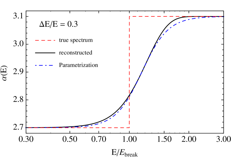
Figure 4: Effects of detector resolution on the shape of the reconstructed energy spectrum. In this example the true spectrum has a sharp knee-like frature at energy $E_{\rm break}$ where the spectral index (indicated by the red, dashed line) changes abruptly from 2.7 to 3.1. The solid line shows the spectral index of the measured spectrum calculated assuming Gaussian errors in the reconstruction of the energy of the events with a resolution $\Delta E/E=0.3$. The (blue) dot–dashed line is the parametrization of the spectral index of Eq. (2) for the “optimum choice”of parameters (see main text).

The observed shape is similar, but not exactly equal to the form of the parametrization in Eq. (2). The asymptotic values of the spectral index for $E\to 0$ and $E\to\infty$ are equal to the true ones, but the energy where the slope of the reconstructed flux is equal to the average value $(\alpha_{2}+\alpha_{1})/2$ is not $E_{b}$ but has a value $E_{b,{\rm rec}}>E_{b}$. This can easily understood as a consequence of the fact already discussed that $\langle E\rangle/E_{\rm rec}<1$. An example of this shift in the position of the break energy, Fig. 5 shows the ratio $E_{b,{\rm rec}}/E_{b}$ plotted as as a function of the detector resolution $\Delta E/E$. For a discontinuity of order $\Delta\alpha\simeq 0.4$ the shift is a factor of order 1.07 for a resolution of 20% and 1.15 for a resolution of 30%.

The detector resolution has also the effect that a very narrow spectral feature is reconstructed as a more gradual softening (or hardening). This effect is illustrated in Fig. 6 that shows the reconstructed width $w_{\rm rec}$ as a function of the detector resolution. The quantity $w_{\rm rec}$ is estimated from Eq. (6) as the width of the energy range where one half of the jump $\Delta\alpha$ develops. For a sharp ($w=0$) break with $\Delta\alpha\simeq 0.4$ one finds that $w_{\rm rec}$ is of order 0.11 for a resolution of 20% and of order 0.15 for a resolution of 30%. The important point here is that, in the absence of systematic effects, is it very unlikely to observe spectral features that are narrower than the width generated by the detector resolution.

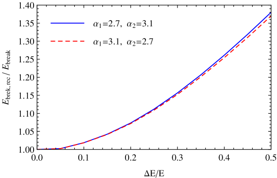
Figure 5: Effects of detector resolution on the shape of a sharp spectral feature The errors on the energy reconstruction are assumed Gaussian with a constant $\Delta E/E$. The curves show the ratio between reconstructed and the true break energy, plotted as as a function of the resolution $\Delta E/E$. The solid curve is for a softening feature (with $\alpha_{1}=2.7$ and $\alpha_{2}=3.1$). The dashed curve for a hardening feature (with $\alpha_{1}=3.1$ and $\alpha_{2}=2.7$).

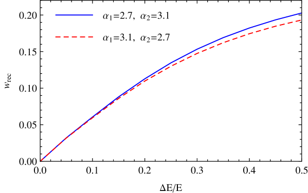
Figure 6: As in Fig. 5. The curves show the reconstructed width $w_{\rm rec}$ as a function of the detector resolution. The solid (dashed) line corresponds to a softening (hardening) spectral feature.

For completeness it should be also added that the detailed shape of an observed spectral feature generated by the detector resolution effects acting on a very narrow structure is not identical (see Fig. 5) to the parametrization of Eq. (1) as it is not exactly symmetric in $\log E_{\rm rec}$, since the evolution in the range $E_{\rm rec}<E_{b,{\rm rec}}$ is slightly faster than the evolution in the range $E_{\rm rec}>E_{b,{\rm rec}}$ (see Fig. 5). This effect is however small and in most cases it can be safely neglected.

In the more general (and realistic case) where a spectral feature has a true width, it is obviously necessary to convolute the detector effects with the real shape of the structure.

3 Two component flux

A simple and natural interpretation of a hardening feature in the cosmic ray spectrum is that the flux is formed by the sum of two components that are reasonably well described in the energy region of the break by power law spectra. In this scenario the flux has the form:

$$\phi(E)=K_{1}\;\left(\frac{E}{E_{0}}\right)^{-\alpha_{1}}+K_{2}\;\left(\frac{E}{E_{0}}\right)^{-\alpha_{2}}$$ (13)

(with $E_{0}$ again an arbitrary reference energy). The two components will be equal at one (unique) crossing energy:

$$E_{\rm cross}=E_{0}\;\left(\frac{K_{1}}{K_{2}}\right)^{1/(\alpha_{1}-\alpha_{2})}$$ (14)

The total flux can be then rewritten in the form:

$$\phi(E)=K_{1}\;\left(\frac{E}{E_{0}}\right)^{-\alpha_{1}}\;\left[1+\left(\frac{E}{E_{\rm cross}}\right)^{-(\alpha_{2}-\alpha_{1})}\right]~{}$$ (15)

This form corresponds exactly to the parametrization of Eq. (1) for the value of the width:

$$w=\frac{1}{\alpha_{1}-\alpha_{2}}~{}$$ (16)

(without loss of generality one can assume that $\alpha_{1}>\alpha_{2}$, so that the first component is the softest one, and therefore $w=(\alpha_{1}-\alpha_{2})^{-1}>0$). Eq. (16) states the (very intuitive) result that the width of a spectral feature that corresponds to the transition between components that have power law form depends on the difference between the spectral indices of the two components, and becomes broader when the two exponents are close to each other. This result can be used to test the hypothesis that a hardening feature is the manifestation of the transition between two components that are unbroken power laws (see the discussion in the following).

4 Spectral features in the CR spectrum

In this section we will very briefly discuss the shape of some of the most prominent features in the flux of protons and of the all–particle spectrum.

We will consider here only the energy range $E\gtrsim 30$ GeV. The discussion of cosmic rays at low energy where the spectra exhibit large and energy dependent curvature, and are also distorted by time dependent solar modulation effect is an important topic, but it will covered here. We also will not discuss the suppression of the CR flux at the highest energies ($E\sim 10^{20}$ eV).

4.1 The Cream/Pamela “discrepant hardening”

An intriguing hardening feature is present in the spectra of protons and helium (and other nuclei) at a rigidity of order 300 GV. The first indication of this hardening emerged indirectly, from a comparison of the spectra measured by the CREAM balloon experiment [3] in the energy range 1–10³ TeV, with the spectra measured at lower energy by magnetic spectrometers such as Caprice [4], BESS [5] and AMS01 [6]. The CREAM collaboration noted that to connect their measurements of the proton and helium spectra to the lower energy data it was necessary to assume the existence of a “discrepant hardening” in the spectra.

Table 1: Parameters of fits to the proton spectrum in the energy range around 1 TeV. The last line is the fit to the AMS02 and CREAM data performed in this work. The fits are shown in Fig. 7.

Experiment	$R_{b}$ (GeV)	$\alpha_{1}$	$\alpha_{2}$	$w$
PAMELA [7]	$232^{+35}_{-30}$	$2.85\pm 0.04$	$2.67\pm 0.05$	$\approx 0$
AMS02 [8]	$336^{+95}_{-52}$	$2.849^{+0.005}_{-0.006}$	$2.716^{+0.075}_{-0.062}$	$0.18^{+0.27}_{-0.18}$
CREAM [10]	–	–	$2.61\pm 0.01$	–
Combined fit	$1010\pm 70$	$2.794\pm 0.003$	$2.57\pm 0.04$	$0.41\pm 0.04$

This prediction received an important confirmation from the measurements of the proton and helium spectra performed by PAMELA [7] that observed hardenings in both spectra at a rigidity of order 230–240 GV.

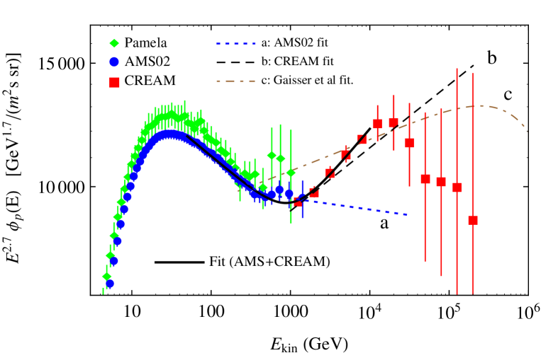
Figure 7: Measurements of the proton flux of Pamela (diamonds) [7]) AMS02 (circles) [8] and CREAM (squares) [10]. The dashed line is the fit of the AMS02 data in the original publication. The solid line is a fit of the combined AMS02 and CREAM data (see main text). The dot–dashed line is the proton flux estimated by Gaisser et al. [11]

Later, the AMS02 detector [8, 9] has also measured the proton and helium spectra with higher precision and in a sligthly broader rigidity range, confirming the existence of the hardenings of the two spectra but measuring a spectral shape not identical to what was obtained by PAMELA. The hardenings measured by AMS02 are centered at higher rigidity, have a smaller $\Delta\alpha$, and a broader width (see table 1).

The data of CREAM, PAMELA and AMS02 on the proton spectrum are shown in Fig. 7. In the case of CREAM the points refer to a recent publication [10] that includes the observations of a second long duration ballon flight. The three collaborations have performed fits to their data that are listed in table 1. The PAMELA collaboration [7] fits the data with is broken power law form (that is a feature with width $w=0$). The AMS02 fit uses the parametrization of Eq. (7), and in table 1 the parameter $w$ is estimated using Eq. (8). The CREAM collaboration [10] fits their data with a simple power law, obtaining a spectral index $\alpha_{p}\simeq 2.61\pm 0.01$. Inspecting Fig. 7 one can however note that there are some indications of a softening of the spectrum for $E\gtrsim 10$ TeV, so that a fit to the data limited to the 1–10 TeV energy range would yield a smaller value of the spectral index.

Comparing the data of the three experiments one can notice that the spectral index measured by CREAM ($\alpha_{p}\simeq 2.61$) is significantly smaller that the asymptotic (high energy) spectral indices fitted by PAMELA ($\alpha_{p}\simeq 2.67$) and AMS02 ($\alpha_{p}\simeq 2.71$). This suggests the possibility that the hardening feature in the proton spectrum is very broad, and extends beyond the rigidity range of the two magnetic spectrometers,

To explore this possibility, we have performed a fit of the AMS02 and CREAM data in the energy range from 50 to $10^{4}$ GeV (a total of 34 data points) using the 5 parameter form of Eq. (1) that describe a single spectral feature. The combination of the AMS02 and CREAM data can be well described by the parametrization of Eq. (1). Combining quadratically statistical and stystematic errors, one obtains $\chi^{2}_{\rm min}=4.9$ (this very small value suggests the existence of significant correlations between the systematic errors for data points at different energies). The best fit parameters are $E_{b}=1011\pm 70$ GeV, $\alpha_{1}\simeq 2.79\pm 0.03$, $\alpha_{2}\simeq 2.57\pm 0.04$ and $w\simeq 0.41\pm 0.04$ (the errors have been estimated using $\chi^{2}<\chi^{2}_{\rm min}+5$). This exercise suggests that it is likely that the proton hardening around one TeV is in fact a very broad feature that extends from 200 GeV to 2 TeV.

The correct description of the proton flux in the energy range 10–100 TeV, is also of great importance as a boundary condition for the studies of the CR flux in the Knee region. Fig. 7 also shows the fit to the proton flux performed by Gaisser et al. [11] taking into account the measurements of the extensive air shower detectors at higher energy.

A discussion of the flux of helium and other nuclei in this energy range is of course very important, but it is postponed to a future work.

4.2 The “Knee”

The prominent structure of the “Knee” in the all–particle spectrum at an energy of order 3 PeV has attracted much attention. It is obvious that to obtain a full understanding of the origin of the knee it is essential to measure separately the energy distributions of the different components (protons, helium nuclei, $\ldots$) that form the spectrum. Estimates of the spectra of different components have been in fact obtained for example by Kascade [12], ARGO–YBJ [13], and Kascade–GRANDE [14, 15, 16], however the determination of the primary particle mass in air shower detectors is difficult and the systematic uncertainties (mostly associated to the modeling of hadronic interactions) are large and poorly understood. A problem of great importance is that the estimates of the proton spectrum in the PeV region by the Kascade and ARGO–YBJ detectors are not in good agreement.

For these reasons it remains interesting to study the detailed shape of the all–particle spectrum. Figure 8 shows some selected measurements of the all–particle spectrum in the energy region from 1 to $10^{3}$ PeV. The data shown is from EAS–TOP [17], TIBET [18], Kascade-Grande [19] and IceTop [20]. The Tibet experiment has presented in [18] three different estimates of the CR flux, obtained using different assumptions for the hadronic interaction model and the particle composition, and the the spectrum shown in Fig. 8 is the one estimated using the Sibyll interaction model [21]).

Inspection of Fig. 8 shows the presence of important differences between the measurements of the different experiments that are the manifestation of the existence of large systematic uncertainties. In fact, a detailed study of how the differences in the reconstructed spectra are related to different methods of measurement, different models of shower development, and different assumptions on the chemical composition of the CR flux, could yield very important information.

Even in the presence of these systematic effects, the measurements of the all–particle flux in the 1–30 PeV energy range reveal the existence of some interesting structure in the shape of the spectrum, that appears to have not one, but two features: a gradual softening centered at $E\simeq 3$–4 PeV, followed by a smaller width hardening at $E\simeq 10$–15 PeV.

The spectra of the different experiments can be well fitted assuming the existence of these two features. A list of the best fit parameters is given in table 2. Note that the EASTOP detector [17] covers only the lower energy part of the knee region, and only observes the spectral softening, while the Kascade–Grande detector [19] covers only the higher energy region, and observes only the hardening. The fits are also shown in Fig. 8.

It is possible that these two (softening and hardening) features in the all–particle spectrum have a distinct origin, however given how close they are, it seems more likely that a physical model that explain these structures will have to address them together, and that what is commonly called “the Knee” should be considered as the combination of these two substructures.

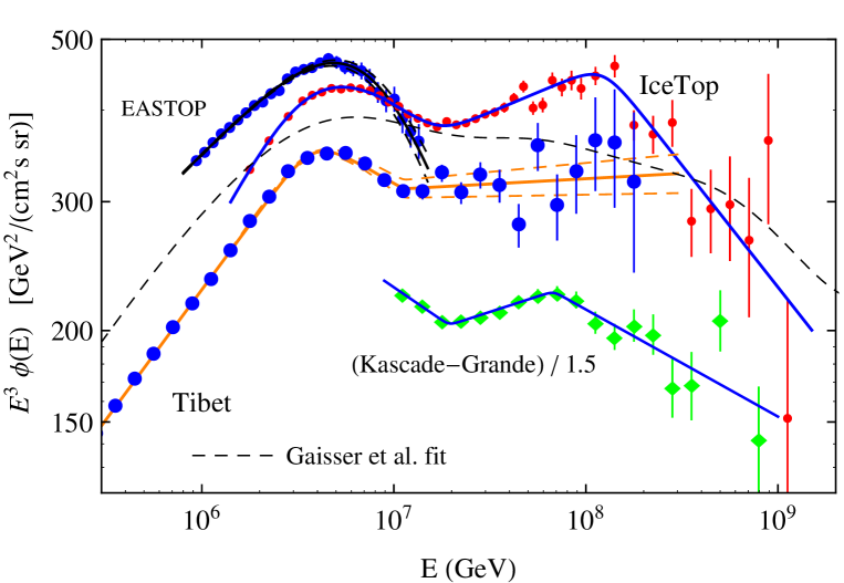
Figure 8: Measurements of the all particle CR spectrum in the energy region $E=10^{6}$–10⁹ GeV by EAS–TOP [17], TIBET [18], Kascade-Grande [19] and IceTop [20]. The lines are fits to the individual measurements using the parametrization of a spectral feature of Eq. (1).

In Fig. 8 we also show the model of the all–particle spectrum constructed by Gaisser et al. [11], where the spectrum of Galactic cosmic rays is modeled as the combinations of three populations of sources that release power law spectra of particles that have rigidity dependent exponential cutoffs at energy 3, 30 and 2000 ($\times Z$) PeV. This type of models is adequate to describe the main features of the spectrum, but the two Knee substructures are not accurately reproduced.

Table 2: Fits to the all–particle CR spectra in the energy range 1–30 PeV. The spectrum is described as three segments where spectral index is approximately constant, with values $\alpha_{1}$, $\alpha_{2}$ and $\alpha_{3}$, separated by two spectral features with break energy $E_{b1}$ and $E_{b2}$ and widths $w_{1}$ and $w_{2}$.

(a) Parameters for the lower energy (softening) feature.

Experiment	$E_{b1}$ (PeV)	$\alpha_{1}$	$\alpha_{2}$	$w_{1}$
EAS–TOP	$7.7\pm 0.3$	$2.73\pm 0.01$	$3.75\pm 0.06$	$0.44\pm 0.02$
TIBET	$3.7\pm 0.6$	$2.62\pm 0.01$	$3.16\pm 0.02$	$0.18\pm 0.02$
IceTop	$3.7\pm 0.3$	$2.50\pm 0.01$	$3.18\pm 0.01$	$0.35\pm 0.01$

(b) Parameters for the higher energy (hardening) feature.

Experiment	$E_{b2}$ (PeV)	$\alpha_{2}$	$\alpha_{3}$	$w_{2}$
TIBET	$11.2\pm 0.2$	$3.16\pm 0.02$	$2.98\pm 0.07$	$<0.15$
IceTop	$17.5\pm 0.7$	$3.18\pm 0.01$	$2.89\pm 0.02$	$0.13\pm 0.01$
Kascade–Grande	$19.4\pm 0.7$	$3.18\pm 0.01$	$2.91\pm 0.02$	$<0.15$

4.3 From the “Knee”to the “Ankle”

The all–particle spectrum in the energy range between the Knee and the Ankle cannot be well fitted as a simple unbroken power law, and there is evidence that the spectrum undergoes some softening.

A structure that has received a lot of attention is the so called “second Knee”, a softening feature observed at $E\approx 300$ PeV by several experiments. This spectral feature is potentially of great significance because it has been identified as possibly marking the transition between Galactic and extragalactic cosmic rays [22].

A review of Bergman and Belz [23] summarizes early results of Akeno, Fly’s Eye and HiRes, obtaining a global best fit for a sharp break centered at $E\simeq 330\pm 15$ PeV where the spectral index undergoes a change $\Delta\alpha\simeq 0.25\pm 0.013$.

More recent data however are not entirely consistent with these conclusions. The Telescope Array Low energy extension (TALE) has recently reported [24] a softening at an energy just below previous estimates $E\simeq 200\pm 23$ PeV, but softening features at lower energy are present in the data of Kascade-Grande [19] (centered at $E\simeq 67\pm 8$ PeV) and IceTop [20] (centered at $E\simeq 123\pm 15$ PeV) The Kascade–Grande and IceTop data, together with our fits are shown in Fig. 8. The HiRes [25] and Telescope Array [26] data, together with our fits centered at 480 and 300 PeV are shown in Fig. 9,

It should be added that if the transition between Galactic and extragalactic cosmic rays is indeed in the region between the Knee and the Ankle, it is virtually certain that it must have a shape that is not well fitted by a simple formula such as Eq. (1).

In fact, a priori one expects that the Galactic/extragalactic transition should correspond to a spectral hardening, simply because the extragalactic flux, that emerges as dominant above the transition energy $E^{*}$, out of hypothesis, must be harder that the Galactic flux, however there is no significant spectral hardening in the energy range 20–4000 PeV.

The transition can correspond to a softening only if three special conditions are satisfied.
(i) The Galactic component has a softening feature at $E_{\rm break}^{\rm Gal}\approx E^{*}$.
(ii) Also the extragalactic component undergoes a softening (presumably with a different astrophysical origin) for $E_{\rm break}^{\rm extra}\approx E^{*}$.
(iii) The two components are normalized so that $\phi_{\rm Gal}(E^{*})\approx\phi_{\rm extra}(E^{*})$.
If these three conditions are satisfied it is then possible to obtain that for $E\lesssim E^{*}$ the CR flux is dominated by the Galactic component before it udergoes its softening; for $E\gtrsim E^{*}$ the flux is dominated by the extragalactic component, after its softening; and around the transition energy $E\approx E^{*}$ one observes a reasonably smooth spectral softening.

As an example, one can consider a simple model where the CR Galactic component is a power law of exponent $\alpha_{0}$ with an exponential (or quasi-exponential) cutoff at $E^{*}_{\rm Gal}$:

$$\phi_{\rm Gal}(E)\simeq K_{\rm Gal}~{}\left(\frac{E}{E_{0}}\right)^{-\alpha_{0}}~{}\exp\left[-\frac{E}{E^{*}_{\rm Gal}}\right]$$ (17)

while the extragalactic flux has a “knee–like” feature at energy $E^{*}_{\rm extra}$:

$$\phi_{\rm extra}(E)\simeq K_{\rm extra}~{}\left(\frac{E}{E_{0}}\right)^{-\alpha_{1}}~{}\left[1+\left(\frac{E}{E^{*}_{\rm extra}}\right)^{\frac{1}{w}}\right]^{-(\alpha_{2}-\alpha_{1})\,w}$$ (18)

If $E^{*}_{\rm Gal}\approx E^{*}_{\rm extra}\simeq E^{*}$ and $K_{\rm extra}/K_{\rm Gal}\approx(E^{*}/E_{0})^{\alpha_{1}-\alpha_{0}}$ (so that the two components are approximately equal for $E\simeq E^{*}$) and if the spectral indices are ordered as: $\alpha_{1}<\alpha_{0},<\alpha_{2}$, the total flux will appear in first approximation as having a softening at $E\simeq E^{*}$ where the spectral index changes from $\alpha_{0}$ (the exponent of the Galactic component before its cutoff) to $\alpha_{2}>\alpha_{0}$ (the exponent of the extragalactic component at high energy). A scenario similar to the one outlined above is in fact a the basis of the “Dip model” of Berezinsky and collaborators [22].

A study of such scenario however shows that a sufficienly accurate measurement of the shape of the spectrum around the transition should show significant deviations from a simple form such as the parametrization of Eq. (1).

4.4 The “Ankle”

The existence of an hardening of the all–particle spectrum at $E\approx 4$–5 EeV has been established already in the 1990’s by Fly’s Eye and Akeno, and these results has been then later confirmed by Haverah Park, Yakutksk, AGASA, HiRes and more recently by Auger and Telescope Array (for reviews see [23, 28, 29].

The interpretation of this spectral feature has already generated a large body of literature. A possibility is that it marks the Galactic/extragalactic CR transition, an alternative [22] is that it is a “dip” created by energy losses effects on a flux of extragalactic protons.

Fig. 9 shows the fit of the spectral shape of the all–particle spectrum performed by Auger [27], and the data of the HiRes [25] and Telescope Array [26] (note that the HiRes data is rescaled by a factor 1/4). The spectra measured by the three experiments exhibit an evident hardening at $E\approx 4$–5 EeV. This spectral feature can be well described by the parametrization of Eq. (1). In fit of the Auger collaboration (see table 3) describes the Ankle as a zero–width spectral break. The results of our fits to the HiRes and Telescope array, performed in the energy range 0.5–40 EeV, are also listed in table 3) and shown in Fig. 9 and yield widths of order 0.23 and 0.12.

Table 3: Parameters of fits to the all–particle spectrum in the Ankle region. The fits are shown in Fig. 9.

Experiment	$E_{a}$ (EeV)	$\alpha_{1}$	$\alpha_{2}$	$w$
Auger [27]	$4.82\pm 0.07\pm 0.8$	$3.29\pm 0.02\pm 0.05$	$2.60\pm 0.02\pm 0.1$	$\approx 0$
HiRes	$5.5^{+0.6}_{-0.4}$	$3.27\pm 0.01$	$2.65\pm 0.07$	$0.23\pm 0.04$
Tel. Array	$4.7^{+0.5}_{-0.4}$	$3.25\pm 0.01$	$2.53\pm 0.09$	$0.12\pm 0.02$

The main point we would like to stress here is that the Ankle is observed as a narrow spectral feature by all experiments, (with stimate of the width of order 0.1–0.3). This result is incompatible with the simplest hypothesis that the spectrum is the superposition of two power law components. As discussed in section 3, in this case the width should be $w\simeq|\Delta\alpha|\approx 1.3$–1.6, that is one order of magnitude larger. As an illustation in Fig. 9 the two dashed lines show the flux obtained as the sum $\phi(E)=K_{1}\;E^{-\alpha_{1}}+K_{2}\;E^{-\alpha_{2}}$ where the two components ($K_{1}\;E^{-\alpha_{1}}$ and $K_{2}\;E^{-\alpha_{2}}$) are the asymptotic forms of the fitted spectrum for energy much smaller and much larger than the Ankle energy. The flux obtained in this way is larger, and has a spectral index that changes much more slowly than the data.

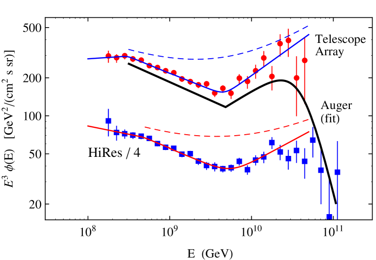
Figure 9: Measurements of the all particle CR spectrum in the energy region $E=10^{8}$–10¹¹ GeV by Telescope Array (circles) [26] and HiRes (squares, divided by a factor 4) [25]. The thick line is the fit of the Auger data [27]. The dashed lines show the flux obtained summing the two asymptotic (for low and high energy) power law spectra obtained with the best fit [$\phi(E)=K_{1}\;E^{-\alpha_{1}}+K_{2}\;E^{-\alpha_{2}}$].

This result does not exclude the hypothesis that the Ankle is created by the transition between regimes where the CR flux is dominated by two different components (for example Galactic and extragalactic particles), however it excludes the possibility that the two components have a simple, unbroken power law form.

5 Conclusions

The identification, and detailed experimental study of the spectral features in the energy distributions of cosmic rays is an essential tool to develop an understanding of the astrophysical mechanisms of acceleration and propagation that determine the fluxes.

A measurement of the width of a spectral feature, that is the range of $\log E$ where the change in spectral index develops, can be a very important constraint for models that want to interpret the CR spectra. It can be useful to have a standard definition for a parameter that measures this property of the spectral features that is commonly accepted. In this work we have suggested the use of a simple and very natural definition for the width of a spectral feature: $w\simeq\Delta\log_{10}E$ (or more precisely $w=\Delta\log_{10}E/\log_{10}9$) where $\Delta\log E$ is the range of $\log E$ where one half of the jump in spectral index of the feature develops.

As an illustration we have discussed three examples of spectral features. The first example is the hardening of the proton flux at $E\simeq 300$ GeV. We find that a simultaneous fit of the AMS02 and CREAM data suggests that this spectral structure is very broad ($w\simeq 0.4$) and centered at high energy ($E_{b}\simeq 1$ TeV). The second example we considered is the well known Knee in the all–particle spectrum at $E\approx 3$–4 PeV. We suggest that this spectral feature should be seen as formed by two substructures, an extended softening at $E\simeq 4$ PeV with a width $w\simeq 0.2$–0.4, followed at $E\simeq 15$–20 PeV by a hardening of narrower width. The third example is the Ankle at $E\simeq 4$ EeV that has a quite small width $w\simeq 0.1$–0.25. This implies that if the Ankle marks the transition between Galactic and extragalactic cosmic rays, it is necessary to assume that at leat one of the two components has significant structure around the transition energy, because the combination of two unbroken power laws would result in a much broader spectral feature.

If the Galactic to extragalactic transition is below the Ankle and corresponds to a softening of the all particle spectrum one expects to find a shape of the energy distribution that, if measured with sufficient accuracy, is not well described by a simple form, because both (Galactic and extragalactic) components must have a non trivial energy dependence.

References

- [1] S. V. Ter–Antonyan and L. S. Haroyan, hep-ex/0003006.
- [2] G. Schatz, Astropart. Phys. 17, 13 (2002). [astro-ph/0104282].
- [3] H. S. Ahn et al., Astrophys. J. 714, L89 (2010). [arXiv:1004.1123 [astro-ph.HE]].
- [4] M. Boezio et al., Astropart. Phys. 19, 583 (2003). [astro-ph/0212253].
- [5] S. Haino et al., Phys. Lett. B 594, 35 (2004). [astro-ph/0403704].
- [6] M. Aguilar et al. [AMS Collaboration], Phys. Rept. 366, 331 (2002).
- [7] O. Adriani et al. [PAMELA Collaboration], Science 332, 69 (2011).
- [8] M. Aguilar et al. [AMS Collaboration], Phys. Rev. Lett. 114, 171103 (2015).
- [9] M. Aguilar et al. [AMS Collaboration], Phys. Rev. Lett. 115, no. 21, 211101 (2015).
- [10] Y. S. Yoon et al., Astrophys. J. 839, no. 1, 5 (2017), [arXiv:1704.02512 [astro-ph.HE]].
- [11] T. K. Gaisser, T. Stanev and S. Tilav, Front. Phys. (Beijing) 8, 748 (2013). [arXiv:1303.3565 [astro-ph.HE]].
- [12] T. Antoni et al. [KASCADE Collaboration], Astropart. Phys. 24, 1 (2005). [astro-ph/0505413].
- [13] B. Bartoli et al. [ARGO-YBJ and LHAASO Collaborations], Phys. Rev. D 92, no. 9, 092005 (2015). [arXiv:1502.03164 [astro-ph.HE]].
- [14] W. D. Apel et al., Astropart. Phys. 47, 54 (2013). [arXiv:1306.6283 [astro-ph.HE]].
- [15] W. D. Apel et al., Phys. Rev. D 87, 081101 (2013). [arXiv:1304.7114 [astro-ph.HE]].
- [16] W. D. Apel et al. Phys. Rev. Lett. 107, 171104 (2011). [arXiv:1107.5885 [astro-ph.HE]].
- [17] M. Aglietta et al. [EAS-TOP Collaboration], Astropart. Phys. 10, 1 (1999).
- [18] M. Amenomori et al. [TIBET III Collaboration], Astrophys. J. 678, 1165 (2008). [arXiv:0801.1803 [hep-ex]].
- [19] W. D. Apel et al., Astropart. Phys. 36, 183 (2012).
- [20] M. G. Aartsen et al. [IceCube Collaboration], Phys. Rev. D 88, no. 4, 042004 (2013). [arXiv:1307.3795 [astro-ph.HE]].
- [21] E. J. Ahn, R. Engel, T. K. Gaisser, P. Lipari and T. Stanev, Phys. Rev. D 80, 094003 (2009). [arXiv:0906.4113 [hep-ph]].
- [22] R. Aloisio, V. Berezinsky, P. Blasi, A. Gazizov, S. Grigorieva and B. Hnatyk, Astropart. Phys. 27, 76 (2007). [astro-ph/0608219].
- [23] D. R. Bergman and J. W. Belz, J. Phys. G 34, R359 (2007). [arXiv:0704.3721 [astro-ph]].
- [24] D. Ivanov, “TA Spectrum Summary,” PoS ICRC 2015, 349 (2016).
- [25] R. U. Abbasi et al. [HiRes Collaboration], Phys. Lett. B 619, 271 (2005). [astro-ph/0501317].
- [26] R. U. Abbasi et al. [Telescope Array Collaboration], Astropart. Phys. 80, 131 (2016). [arXiv:1511.07510 [astro-ph.HE]].
- [27] Inés Valino [for the Pierre Auger Collaboration], arXiv:1509.03732 [astro-ph.HE].
- [28] J. Blumer, R. Engel and J. R. Horandel, Prog. Part. Nucl. Phys. 63, 293 (2009) [arXiv:0904.0725 [astro-ph.HE]].
- [29] G. Matthiae and V. Verzi, Riv. Nuovo Cim. 38, no. 2, 73 (2015).