Nonlinear dynamics of damped DNA systems with long-range interactions

Abstract

We investigate the nonlinear dynamics of a damped Peyrard-Bishop DNA model taking into account long-range interactions with distance dependence $|l|^{-s}$ on the elastic coupling constant between different DNA base pairs. Considering both Stokes and long-range hydrodynamical damping forces, we use the discrete difference operator technique and show in the short wavelength modes that the lattice equation can be governed by the complex Ginzburg-Landau equation. We found analytically that the technique leads to the correct expression for the breather soliton parameters. We found that the viscosity makes the amplitude of the breather to damp out. We compare the approximate analytic results with numerical simulations for the value $s=3$ (dipole-dipole interactions).

1 Introduction

The DNA molecule is known to be very important and essential in the protection, transport and transmission of the genetic code. Many theoretical models have been proposed to describe the nonlinear dynamics of DNA. The first nonlinear DNA model was suggested by Englander et al. [2]. Thereafter, simplified models were proposed to describe the angular distortion of DNA [3, 4, 5] and the micromanipulation experiments were investigated, showing the great importance of radial displacements of bases during the processes of replication and transcription [6, 7, 8]. The Peyrard-Bishop (PB) DNA model [6], which has been successfully used to analyze experiments on short DNA sequences [9] has gained a popularity in that direction.

DNA double helix spontaneously denatures locally and the breathing mode occurs when it is locally excited with large amplitude [10]. The amplitude of this excitation depends on the surrounding environment-DNA interactions and the inner mechanism of the DNA molecule depending on the relative motion of particles. It is therefore of physical importance to take into account these two effects in the nonlinear dynamics of DNA molecule. Some authors emphasized the influence of the viscosity on the dynamical properties of the DNA molecule [11, 12]. In particular, it is shown that the viscosity of the medium damps out the amplitude of the nonlinear wave propagating through the molecule [11, 12]. In the above studies, the analysis deal with the PB DNA model with nearest neighbor interactions between base pairs. The long-range interactions (LRI) play a crucial role in molecular systems [13, 14, 15]. The importance of LRI in DNA molecule is due to the presence of phosphate groups along the strands [13]. The LRI therefore allow to take into account the screening of the interactions or an indirect coupling between base pairs (e.g. via water filaments) [14]. Rau and Parsegian, in their experimental studies in the direct measurements of the intermolecular forces between counterion-condensed DNA double helices, have shown the importance of long-range attractive hydrogen forces and emphasize that many forces could be responsible for LRI in the DNA molecule [15]. In fact, the charged groups in the molecular chains and DNA molecules interact through long-range dipole-dipole interactions. Along the same line, it has been shown that the study of the power-law LRI in nonlinear lattice models is very relevant mainly in molecular chains and DNA molecules where Coulomb and dipole-dipole interactions are of a great physical importance [16, 17, 18]. Recent works by Mvogo et al. [19, 20] also indicated qualitative effects of the power-law LRI in molecular systems.

To the best of our knowledge, no work has been reported on the study of DNA dynamics taking into account both damping and LRI effects. Our aim in this paper is to study the DNA dynamics taking into account LRI between different DNA base pairs and both Stokes and long-range hydrodynamical damping effects. To address this issue, our analytical study has been inspired by the one recently developed by Miloshevich et al. [21] to investigate traveling solitons in long-range oscillator chains. Due to the non analytical properties of the dispersion relation, Miloshevich et al. [21] have shown that the discrete difference operator (DDO) technique is more appropriate to study physical systems with LRI. In this paper, we use the DDO and show that the DNA models with LRI can be reduced to a specific form of the complex Ginzburg-Landau (CGL) equation, where the dispersion coefficient is complex and the nonlinearity coefficient is real. A similar equation has been obtained by Zdravkovíc et al. [11, 12] while studying the effect of viscosity on the dynamics of the Peyrard-Bishop-Dauxois (PBD) DNA model in the absence of hydrodynamical damping and LRI forces. The investigators state that the CGL equation cannot be solved analytically like a nonlinear Schrodinger (NLS) equation [11, 12]. In this paper, following the work by Pereira and Stenflo [22], we analytically solve the CGL equation.

The paper is organized as follows. In Section 2, we propose the Hamiltonian model and derive the discrete equations of motion for the in-of-phase and out-of-phase motions. In Section 3, we use the DDO and show that the out-of-phase dynamical equation can be reduced to the CGL equation. The envelope soliton solution of this equation is reported and the breather solution of the discrete equation of motion for the out-of-phase motion is derived. In Section 4, we perform the numerical simulations with emphasis on the effects of the LRI and damping forces. Section 5 concludes the work.

2 Model and equations of motion

We consider the PB model [6] for DNA denaturation where the degrees of freedom $x_{n}$ and $y_{n}$ associated to each base pair correspond to the displacements of the bases from their equilibrium positions along the direction of the hydrogen bonds that connect the two bases in a pair. A LRI coupling between the base pairs due to the presence of phosphate group along the DNA strands is assumed so that the Hamiltonian for the model is given by

$$\begin{split}H=&\sum\limits_{n}^{N}\Big{\{}\frac{1}{2}m(\dot{x}_{n}^{2}+\dot{y}_{n}^{2})+\frac{1}{2}\sum\limits_{l=1}J_{l}[(x_{n}-x_{n-l})^{2}+(y_{n}-y_{n-l})^{2}]+V(x_{n},y_{n})\Big{\}},\end{split}$$ (1)

where $m$ is the average mass of the nucleotides and $N$ represents the number of the base pairs of the DNA molecule. The interactions between hydrogen bonds in a pair is modeled by the Morse potential $V(x_{n},y_{n})$ given by

$$V(x_{n},y_{n})=D\left[e^{-a(x_{n}-y_{n})}-1\right]^{2},$$ (2)

where $D$ is the depth of the Morse potential well, which may depend on the type of base pair and $a$ is the width of the well. The quantity

$$J_{l}=J|l|^{-s},$$ (3)

is the power-law dependence of the elastic coupling constant, where $s$ and $|l|$ are the LRI parameter and the normalized distance between base pairs, respectively. In practice, to keep the spatial homogeneity in a finite DNA system with periodic boundary conditions, usually the LRI is limited in each direction to $\frac{1}{2}(N-1)$, if $N$ is odd, or $\frac{1}{2}(N-2)$, if $N$ is even, and $1\leq|l|\leq\frac{1}{2}(N-1)$ [23]. The parameter $s$ can be used to model Coulomb interactions between charged particles of a chain ($s=1$), dipole-dipole interactions ($s=3$). Below $s=1$ the energy diverges and above $s=3$ the system becomes short-range. In this paper, we use the case $s=3$, where multiple solutions exist [24].

The values of parameters used to perform our analysis are those from the dynamical and denaturation properties of DNA. They are [25]: $m=300$ amu, $J=0.06$ eV/Ų, $D=0.03$ $eV$ and $a=4.5$ Å^-1. Our system of units (amu, Å, eV) defines a time unit ($t.u.$) equal to $1.018\times 10^{-14}$ s.

To describe the motions of the two strands, we introduce the new variables $u_{n}$ and $v_{n}$ such that

$$u_{n}=\frac{x_{n}+y_{n}}{\sqrt{2}}\;\ \mathrm{and}\;\ v_{n}=\frac{x_{n}-y_{n}}{\sqrt{2}},$$ (4)

where $u_{n}$ and $v_{n}$ represent the in-phase and the out-of-phase motions. Taking into account Eq. (2) and Eq. (4), the Hamiltonian of the system can be rewritten as

$$\begin{split}H=&\sum\limits_{n}^{N}\Big{\{}\frac{1}{2}m\dot{u}_{n}^{2}+\frac{1}{2}\sum\limits_{l=1}J_{l}(u_{n}-u_{n-l})^{2}\Big{\}}+\sum\limits_{n}^{N}\Big{\{}\frac{1}{2}m\dot{v}_{n}^{2}+\frac{1}{2}\sum\limits_{l=1}J_{l}(v_{n}-v_{n-l})^{2}+D\left(e^{-a\sqrt{2}v_{n}}-1\right)^{2}\Big{\}}.\end{split}$$ (5)

The equations of motions of the system then read

$$m\ddot{u}_{n}=\sum\limits_{l=1}J_{l}\left(u_{n+l}-2u_{n}+u_{n-l}\right),$$ (6)

$$\begin{split}m{\ddot{v}_{n}}=&\sum\limits_{l=1}J_{l}\left(v_{n+l}-2{v_{n}}+v_{n-l}\right)+2\sqrt{2}aDe^{-a\sqrt{2}v_{n}}\left(e^{-a\sqrt{2}v_{n}}-1\right).\end{split}$$ (7)

For a more realistic study of dynamical properties of DNA, one must take into account its environment. In the present work, we take into account the Stokes ($F^{st}$) and the long-range hydrodynamical ($F^{hy}$) damping forces in the equations of motion of the system. These forces account respectively for DNA molecules in a viscous environment and their inner mechanism. The Stokes damping forces is given by

$$F_{n}^{st}=-m\gamma^{st}\dot{q}_{n},$$ (8)

where $\gamma^{st}$ is the Stokes damping constant. The coordinate $q_{n}$ can be replaced by $u_{n}$ or $v_{n}$. In previous works in discrete lattices, investigators assume the hydrodynamical damping force in the nearest neighbor interactions [26, 27, 28, 29]. In this work, the DNA molecule is considered as a collection of nucleotides linked to the neighbors of the same strand by spring. Each of them is assumed to be point masses of mass $m$. Thus, the displacement of one base pair causes a more or less significant displacement of the other base pairs of the chain according to whether they are closed or distanced from the initial base pair. This displacement gives rise to the hydrodynamical viscous forces which influence the motion of the initial nucleotide. Since our work focuses on LRI between base pairs, we have introduced the LRI in the hydrodynamic dissipation $F^{hy}$ in order to takes into account the contribution of all base pairs of the chain so that,

$$F_{n}^{hy}=m\sum\limits_{l=1}\gamma_{l}\left(\dot{q}_{n-l}-2\dot{q}_{n}+\dot{q}_{n+l}\right),$$ (9)

where $\gamma_{l}=\gamma^{hy}|l|^{-s^{\prime}}$ and $\gamma^{hy}$ is the hydrodynamical damping coupling constant. Taking into account $F_{n}^{st}$ and $F_{n}^{hy}$ as defined above, we obtain the following equations of motion:

$$\begin{split}\ddot{u}_{n}=&\sum\limits_{l=1}\frac{J_{l}}{m}(u_{n+l}-2u_{n}+u_{n-l})-\gamma^{St}\dot{u}_{n}+\sum\limits_{l=1}\gamma_{l}\left(\dot{u}_{n+l}-2\dot{u}_{n}+\dot{u}_{n-l}\right)\end{split}$$ (10)

$$\begin{split}\ddot{v}_{n}=&\sum\limits_{l=1}{\frac{J_{l}}{m}}(v_{n+l}-2v_{n}+v_{n-l})+\frac{2\sqrt{2}aD}{m}e^{-a\sqrt{2}v_{n}}(e^{-a\sqrt{2}v_{n}}-1)-\gamma^{St}\dot{v}_{n}+\sum\limits_{l=1}\gamma_{l}\left(\dot{v}_{n+l}-2\dot{v}_{n}+\dot{v}_{n-l}\right).\end{split}$$ (11)

The solution $u_{n}(t)$ of Eq. (10) is an ordinary solution of a damped linear schrödinger equation and represents a plane wave in a viscous medium in the presence of LRI. In what follows, the system will be considered heavily damped. Our investigations will be limited to the analysis of the dynamical behavior of the stretching motion of each base pair represented by the solution of Eq. (11), in the presence of LRI and the “big viscosity ”  [11, 12].

3 Discrete difference operator technique

In this section, the DDO technique which is appropriate for long-range interacting systems [21] is used to study the dynamics of DNA breathing. Assuming as usual small amplitude oscillation of the nucleotide around the bottom of the Morse potential, we obtain up to the third order of the Morse potential the following equation of motion:

$$\begin{split}\ddot{v}_{n}=&\sum\limits_{l=1}{\frac{J_{l}}{m}}(v_{n+l}-2v_{n}+v_{n-l})-\omega_{g}^{2}(v_{n}+\alpha v_{n}^{2}+\beta v_{n}^{3})-\gamma^{St}\dot{v}_{n}+\sum\limits_{l=1}\gamma_{l}\left(\dot{v}_{n+l}-2\dot{v}_{n}+\dot{v}_{n-l}\right).\end{split}$$ (12)

where $\omega_{g}^{2}=\frac{4a^{2}D}{m}$, $\alpha=-\frac{3a}{\sqrt{2}}$ and $\beta=\frac{7a^{2}}{3}$. Eq. (12) describes the dynamics of the out-of-phase motion of the DNA in viscous medium in the presence of LRI forces. Introducing the distance of neighboring bases $r$ and assuming plane wave solutions of the form

$$\begin{split}v_{n}=F_{1}e^{i(qnr-\omega t)}+c.c.\end{split}$$ (13)

and substituting them into the equations of motion, we obtain the nonlinear dispersion relation in rotating wave approximation for the normal mode frequencies $\omega_{n}$ and wave numbers $q_{n}$

$$\omega_{n}^{2}=\omega_{g}^{2}(1+3\beta|F_{1}|^{2})+4\sum\limits_{l=1}\frac{J_{l}}{m}\sin^{2}(q_{n}^{0}lr/2)-i\omega_{n}\gamma_{n},$$ (14)

where $\gamma_{n}$ is the damping coefficient given by:

$$\gamma_{n}=\gamma^{st}+4\sum\limits_{l=1}\gamma_{l}\sin^{2}(q_{n}^{0}rl/2).$$ (15)

After some algebras, this dispersion relation can be rewritten as the sum of its real part $\omega_{r}$ and imaginary part $\omega_{i}$. That is

$$\begin{split}\omega_{n}=\omega_{r}+i\omega_{i},\qquad\omega_{r}=\omega_{0,n}\sqrt{1-\delta_{n}^{2}},\qquad\omega_{i}=-\frac{\gamma_{n}}{2},\\ \end{split}$$ (16)

with $\delta_{n}=\frac{\gamma_{n}}{2\omega_{0,n}}$ and $\omega_{0,n}$ the optical frequency of vibrations of base pairs in the absence of damping forces given by

$$\begin{split}\omega_{0,n}^{2}=\omega_{g}^{2}(1+3\beta|F_{1}|^{2})+4\sum\limits_{l=1}\frac{J_{l}}{m}\sin^{2}(q_{n}^{0}rl/2).\end{split}$$ (17)

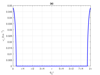
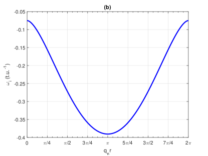
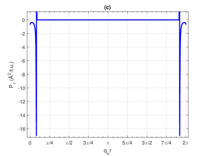
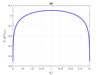
Figure 1: (Color online) (a) and (b) the real and imaginary part of the dispersion relation (Eq. (16)) in the linear limit $F_{1}\rightarrow 0$. (c) and (d) the real and imaginary part of the second discrete derivative of the dispersion relation (Eq. (29)) (Dispersion coefficient) in terms of the discretized values of the wave vector $q_{n}r=2\pi n/N$, $N=600$ for $s=3.00$, $\gamma_{0}=0.15$ $t.u^{-1}$.

We plot in Figure 1 the real and imaginary parts of the angular frequency of the wave (Eq. (16)), the real and imaginary parts of the dispersion coefficient in the linear limit $|F_{1}|\rightarrow 0$ for discretized values of the wave vector $q_{n}^{0}r$ for $s=3.00$ and $\gamma_{0}=0.15$. In the panel (a) we observe that the real part of the angular frequency is equal to zero for $q_{n}r\in]\frac{\pi}{12},\frac{23\pi}{12}[$ and different from zero otherwise, namely $q_{n}r\in[0,\frac{\pi}{12}]$ and $q_{n}r\in[\frac{23\pi}{12},2\pi]$. Then the vibration can appears and propagates in the DNA molecule only if the carrier wave vector $q_{n}r$ is selected in a finite interval $\Big{\{}[0,\frac{\pi}{12}]$ $\cup$ $[\frac{23\pi}{12},2\pi]\Big{\}}$.

The contribution of the long range decays of the stacking and viscous interactions are not the same, since the origins of the two forces are physically different, but nevertheless for seek of simplicity the same exponent is assumed that is $s=s^{\prime}$. Also, as in [30], we set $\gamma_{0}=\gamma^{st}=\gamma^{hy}$. At small wavelength, the soliton solution of Eq. (12) is found as an expansion in normal modes and may be found in the form [31].

$$\begin{split}v_{n}=\varepsilon[F_{1}(z_{1},\tau)e^{i(q^{0}rn-\omega^{0}t)}+c.c.],\end{split}$$ (18)

with

$$\begin{split}F_{1}(z_{1},\tau)=\sum\limits_{n=1}^{N}B_{n}e^{i(\delta q_{n}z_{1}-\delta\omega_{n}\tau)},\qquad q_{n}=q^{0}+\varepsilon\delta q_{n},\qquad\omega_{n}=\omega^{0}+\varepsilon^{2}\delta\omega_{n}.\end{split}$$ (19)

The function $F_{1}$ is a slowly varying function in space $z_{1}=\varepsilon rn$ and time $\tau=\varepsilon^{2}t$. The parameter $q^{0}$ is the wavenumber of the wave packet and the associate frequency $\omega^{0}\equiv\omega(q^{0},F_{1}=0)$ in the limit $F_{1}\rightarrow 0$

The time derivative of the wave amplitude Eq. (19) reads:

$$\begin{split}\frac{\partial F_{1}(z_{1},\tau)}{\partial\tau}=[-i\delta\omega_{n}]\sum\limits_{n=1}^{N}B_{n}e^{i(\delta q_{n}z_{1}-\delta\omega_{n}\tau)}=[-i\delta\omega_{n}]F_{1}.\end{split}$$ (20)

From Eqs. (14), (19) and (18) it is seen that the term $\varepsilon^{2}\delta\omega_{n}$ is an evolution function of two variables: the wavenumber $q^{0}$ and the slowly varying wave amplitude $|\varepsilon F_{1}|^{2}$. The Taylor expansion of this term around the value $q^{0}$ and $|\varepsilon F_{1}=0|$ and neglecting higher order terms $(>2)$, give us

$$\begin{split}\varepsilon^{2}\delta\omega_{n}(\partial q_{n},|\varepsilon F_{1}|^{2})=\delta\omega^{0}(q^{0})+(q_{n}-q^{0})\frac{\partial\omega^{0}(q^{0})}{\partial q^{0}}+\frac{1}{2}(q_{n}-q^{0})^{2}\frac{\partial^{2}\omega^{0}(q^{0})}{(\partial{q^{0}})^{2}}+|\varepsilon F_{1}|^{2}\frac{\partial\omega_{n}(q^{0})}{\partial(|F_{1}|^{2})}\Big{|}_{F_{1}=0}.\end{split}$$ (21)

The first term of the right hand site of Eq. (21) is assuming to be very close to zero. From Eq. (19) we have $\varepsilon\delta q_{n}=q_{n}-q^{0}$. The above considerations in Eq. (21) lead to:

$$\begin{split}\delta\omega_{n}(\partial q_{n},|F_{1}|^{2})=\frac{(\varepsilon\delta q_{n})}{\varepsilon^{2}}\frac{\partial\omega^{0}(q^{0})}{\partial q^{0}}+\frac{1}{2}\frac{(\varepsilon\delta q_{n})^{2}}{\varepsilon^{2}}\frac{\partial^{2}\omega^{0}(q^{0})}{\partial{q^{0}}^{2}}+|F_{1}|^{2}\frac{\partial\omega_{n}(q^{0})}{\partial(|F_{1}|^{2})}\Big{|}_{F_{1}=0}.\end{split}$$ (22)

The discrete difference operator is used instead of the continuous derivatives which can cause divergences. Therefore we have:

$$\begin{split}\frac{\partial\omega^{0}(q^{0})}{\partial q^{0}}=\frac{\omega^{0}(q^{0}+h)-\omega^{0}(q^{0})}{h},\qquad\frac{\partial^{2}\omega^{0}(q^{0})}{\partial{q^{0}}^{2}}=\frac{\omega^{0}(q^{0}+h)-2\omega^{0}(q^{0})+\omega^{0}(q^{0}-h)}{h^{2}},\end{split}$$ (23)

and finally we get,

$$\begin{split}\delta\omega_{n}(\partial q_{n},|F_{1}|^{2})=\sum\limits_{\nu=1}^{2}\frac{(\varepsilon\delta q_{n})^{\nu}}{\varepsilon^{2}\nu!}\frac{\Delta_{h}^{(\nu)}[\omega^{0}(q^{0})]}{h^{\nu}}+|F_{1}|^{2}\frac{\partial\omega_{n}(q^{0})}{\partial(|F_{1}|^{2})}\Big{|}_{F_{1}=0},\end{split}$$ (24)

where $\Delta^{(\nu)}_{h}$ is the difference operator of order $\nu$ with step size $h=2\pi/N$ in the limit $F_{1}=0$ and given below,

$$\begin{split}\Delta^{(1)}_{h}[\omega^{0}]=\omega^{0}(q^{0}+h)-\omega^{0}(q^{0}),\qquad\Delta^{(2)}_{h}[\omega^{0}]=\omega^{0}(q^{0}+h)-2\omega^{0}(q^{0})+\omega^{0}(q^{0}-h).\end{split}$$ (25)

From Eq. (19) the term $(\delta q_{n})^{\nu}$ can be expressed as follows:

$$\begin{split}(i\delta q_{n})^{\nu}F_{1}=\frac{\partial^{\nu}F_{1}}{\partial z_{1}^{\nu}}.\end{split}$$ (26)

Using Eqs. [26-23] into Eq. (20) give the nonlinear equation of evolution of the envelope function written as

$$\begin{split}i\Big{[}\frac{\partial F_{1}}{\partial\tau}+\frac{v_{g}}{\varepsilon}\frac{\partial F_{1}}{\partial z_{1}}\Big{]}+P\frac{\partial^{2}F_{1}}{\partial z^{2}}+Q|F_{1}|^{2}F_{1}=0\end{split}$$ (27)

where the parameters $v_{g}$, $P$ and $Q$ are the group velocity, the dispersion and the nonlinearity coefficients given by

$$\begin{split}v_{g}=\frac{\Delta^{(1)}_{h}[\omega^{0}]}{h},\qquad P=\frac{\Delta^{(2)}_{h}[\omega^{0}]}{2h^{2}},\qquad Q=-\frac{\partial\omega_{n}(q^{0})}{\partial(|F_{1}|^{2})}\Big{|}_{F_{1}=0}.\end{split}$$ (28)

The above parameters can be rewritten as:

$$\begin{split}&v_{g}=v_{gr}+iv_{gi},\qquad v_{gr}=\frac{\Delta^{(1)}_{h}[\omega_{r}^{0}]}{h},\qquad v_{gi}=\frac{\Delta^{(1)}_{h}[\omega_{i}^{0}]}{h}\\ &P=P_{r}+iP_{i},\qquad P_{r}=\frac{\Delta^{(2)}_{h}[\omega_{r}^{0}]}{2h^{2}},\qquad P_{i}=\frac{\Delta^{(2)}_{h}[\omega_{i}^{0}]}{2h^{2}},\\ &Q=Q_{r}+iQ_{i},\qquad Q_{r}=-\frac{3\beta\omega_{g}^{2}}{2\omega_{r}^{0}},\qquad Q_{i}=0.\end{split}$$ (29)

Setting $\xi_{1}=z_{1}-\varepsilon v_{g}t$ in the co-moving reference frame with a rescaled time $t$ such as $t\rightarrow\varepsilon^{2}t$, Eq. (24) becomes

$$\begin{split}i\frac{\partial F_{1}}{\partial t}+(P_{r}+iP_{i})\frac{\partial^{2}F_{1}}{\partial\xi_{1}^{2}}+Q|F_{1}|^{2}F_{1}=0.\end{split}$$ (30)

It should be noted that Eq. (30) is the well-known CGL equation for the evolution of the envelope where the dispersion coefficient is complex and the nonlinearity coefficient is real. Similar equation was found in Ref. [11, 12] where the authors studied the dynamics of a damped DNA in the absence of hydrodynamical damping and LRI forces using the semi-discrete approximation. In their study they found the dispersion coefficient real and the nonlinearity coefficient complex contrary of the one obtained in this work. The nonlinearity coefficient $Q$ and the dispersion coefficient $P$ not only depend on the wave vector $q_{n}^{0}r$, and the Stokes viscous forces as previously mentioned by these authors, but also depend on the hydrodynamic damping and the LRI forces.

Several methods related to soliton solutions for the specific forms of CGL equation have been developed [22, 32, 33]. A key problem in this paper is to give an analytical soliton solution of the CGL equation (Eq. (30)), and use it to study the effect of viscosity and LRI on the DNA opening state configuration. The character of this solution is determined by the sign of $Q$ and $P_{r}$ while the stability of the plane wave solution through the Benjamin-Feir instability depends on the sign of the product $P_{r}Q$. For $P_{r}Q<0$, the plane wave solution is stable and for $P_{r}Q>0$ it is unstable. Particularly, since the nonlinear coefficient $Q$ is always negative the sign of the constant $P_{r}Q$ depends on real part of the dispersion coefficient $P_{r}$ which can take positive or negative values depending on the range of variations of the wave vector. Here, only localized solutions in space for any wave carrier whose wavenumber is in the positive range of $P_{r}Q$ are considered.

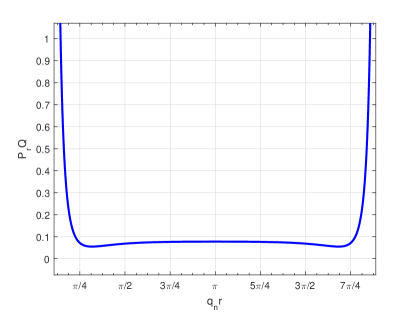
Figure 2: (Color online) The product $PrQ$ in terms of the the discretized values of the wave vector $q_{n}r=2\pi n/N$, $N=600$, for $s=3.00$, $\gamma_{0}=0.15$ $t.u^{-1}$

In Figure 2, the product $P_{r}Q$ is represented as a function of the wave vector for $s=3.00$ and $\gamma=0.15$. We observe in the plots that $P_{r}Q>0$ is always positive. From Eqs. (15), (16) and (29), we observe that the imaginary parts of the solitonic parameters strongly depend on the damping forces of the system, therefore their absolute values decrease with the decreasing of the damping constant and vanish when the damping is switched off.

As in [22, 32, 33], an analytical solution of Eq. (31), is found in the form

$$\begin{split}&F_{1}=A\Big{[}\mbox{{$\,$sech}}(\eta\xi_{1})\Big{]}^{1+i\sigma}e^{-i\phi t},\\ \end{split}$$ (31)

where $A$, $\phi$, $\eta^{-1}$, and $\sigma$ are parameters to be determined and represent respectively the complex amplitude, the complex “angular frequency ”, the width and the chirp of the soliton. By introducing Eq. (31) into Eq (30) and after canceling the terms in $[\mbox{{$\,$sech}}(\eta\xi_{1})\Big{]}^{1+i\sigma}$, the real and imaginary part of the phase of the soliton is written

$$\begin{split}&\phi_{r}=-\eta^{2}\Big{[}(1-\sigma^{2})P_{r}-2\sigma P_{i}\Big{]},\qquad\phi_{i}=-\eta^{2}\Big{[}(1-\sigma^{2})P_{i}+2\sigma P_{r}\Big{]}.\end{split}$$ (32)

From the annihilation of the terms in $[\mbox{{$\,$sech}}(\eta\xi_{1})\Big{]}^{3+i\sigma}$, the width and the chirp of the soliton is given by

$$\begin{split}&|A|=\eta\sqrt{\Big{|}\frac{(2-\sigma^{2})P_{r}-3\sigma P_{i}}{Q_{r}}}\Big{|},\qquad\sigma=\frac{3P_{r}+\sqrt{\Delta}}{2P_{i}}\\ \end{split}$$ (33)

where $\Delta=9P_{r}^{2}+8P_{i}^{2}$ and $\sigma$ a solution of the following quadratic equation

$$\begin{split}&P_{i}\sigma^{2}-3P_{r}\sigma-2P_{i}=0.\end{split}$$ (34)

This choice of $\sigma$ implies that the soliton is strongly chirped.

Now to determine the complex amplitude $A_{\gamma}$ of the soliton, let us consider the system in the non-viscous limit ($\gamma_{0}=0$). In that case $P_{i}$ vanishes and Eq. (30) becomes the standard NLS equation

$$i\frac{\partial G_{1}}{\partial t}+P^{\prime}\frac{\partial^{2}G_{1}}{\partial\xi_{1}^{2}}+Q^{\prime}|G_{1}|^{2}G_{1}=0,$$ (35)

where the associated group velocity, dispersion coefficient and nonlinearity coefficient are

$$\begin{split}v_{g}^{\prime}\equiv v_{gr}\Big{|}_{\gamma=0}=\frac{\Delta^{(1)}_{h}[\omega_{0}^{0}]}{h},\qquad P^{\prime}\equiv P_{r}\Big{|}_{\gamma=0}=\frac{\Delta^{(2)}_{h}[\omega_{0}^{0}]}{2h^{2}},\qquad Q^{\prime}\equiv Q_{r}\Big{|}_{\gamma=0}=-\frac{3\beta\omega_{g}^{2}}{2\omega_{0}}.\end{split}$$ (36)

The solution of Eq. (35) is the well known modulated solitonic wave called breather [25, 34] and given by

$$\begin{array}[]{l}G_{1}=A^{\prime}\mbox{{$\,$sech}}\Big{[}L(\xi_{1}-u_{e}t)\Big{]}e^{i\frac{u_{e}}{2P^{\prime}}(\xi_{1}-u_{c}t)},\end{array}$$ (37)

where $u_{e}$ and $u_{c}$ are real parameters representing respectively the velocities of the envelope and the carrier wave of the soliton. The amplitude of the envelope $A^{\prime}$ and its inverse width $L^{\prime}$ are given by the relations

$$\begin{split}L^{\prime}=\frac{\sqrt{u_{e}^{2}-2u_{e}u_{c}}}{2P^{\prime}},\qquad A^{\prime}=\sqrt{\frac{u_{e}^{2}-2u_{e}u_{c}}{2P^{\prime}Q^{\prime}}}.\end{split}$$ (38)

Let us assume that at the initial time ($t=0$), for $\gamma_{0}=0$, the soliton solution Eqs. (31) and (38) should be equivalent,

$$\begin{array}[]{l}A\Big{|}_{\gamma=0}=A^{\prime}e^{i\frac{u_{e}}{2P^{\prime}}\xi_{1,0}},\end{array}$$ (39)

where $\xi_{1,0}$ is the initial position of the soliton. Taking into account this new expression of the amplitude $A$, the one soliton solution of Eq. (30) is

$$\begin{split}&F_{1}=\eta\sqrt{\Big{|}\frac{(2-\sigma^{2})P_{r}-3\sigma P_{i}}{Q_{r}}}\Big{|}e^{\phi_{i}t}\Big{[}\mbox{{$\,$sech}}(\eta\xi_{1})\Big{]}^{1+i\sigma}e^{i(\frac{u_{e}}{2P}\xi_{1,0}-\phi_{r}t)}.\end{split}$$ (40)

Now considering the fact that the angular frequency of the soliton is complex (see Eq. (16)), one can note that the term $e^{\omega_{i}t}$ enters inside the amplitude of the soliton. Thus, the complete expression of the envelope soliton written in the original temporal ($t$) and spacial ($z$) variables is finally given by

$$\begin{split}F^{\prime}_{1}=&F_{1}e^{\omega_{i}t}=\eta\sqrt{\Big{|}\frac{(2-\sigma^{2})P_{r}-3\sigma P_{i}}{Q_{r}}}\Big{|}e^{-\Gamma t}\Big{[}\mbox{{$\,$sech}}\big{[}\eta(z_{1}-\varepsilon v_{gr}t)\big{]}\Big{]}^{1+i\sigma}e^{i\Theta}\\ \end{split}$$ (41)

with

$$\begin{split}\Theta=&\frac{u_{e}}{2P}\xi_{1,0}+\eta^{2}\Big{[}(1-\sigma^{2})P_{r}-2\sigma P_{i}\Big{]}t,\qquad\Gamma=\frac{\gamma_{n}}{2}+\eta^{2}\Big{[}(1-\sigma^{2})P_{i}+2\sigma P_{r}\Big{]},\qquad\eta=\frac{\sqrt{u_{e}^{2}-2u_{e}u_{c}}}{\Big{|}(2-\sigma^{2})P_{r}-3\sigma P_{i}\Big{|}}\end{split}$$ (42)

where $\Gamma$ is the effective damping constant of the medium.

To obtain the solution of the EOM of the out-of-phase motion $v_{n}$ given by Eq. (11), some results of the previous section are used. Using Eqs. (16), (28) and (40) the soliton solution describing the out-of-phase motion of the DNA in the viscous medium takes the form

$$\begin{split}v_{n}(t)=&2\varepsilon|A|e^{-\Gamma t}\mbox{{$\,$sech}}\big{[}\varepsilon\eta(nr-v_{gr}t)\big{]}\cos(q_{\gamma}nr-\varpi t)\end{split}$$ (43)

where

$$\begin{split}&\varpi=\omega_{r}^{0}-\eta^{2}\Big{[}(1-\sigma^{2})P_{r}-2\sigma P_{i}\Big{]},\qquad q_{\gamma}=q^{0}+\frac{u_{e}}{2P}\Big{(}\frac{\xi_{1,0}}{nr}\Big{)}+(\sigma/nr)\log\Big{|}\mbox{{$\,$sech}}\big{[}\varepsilon\eta(nr-v_{gr}t)\big{]}\Big{|}.\\ \end{split}$$ (44)

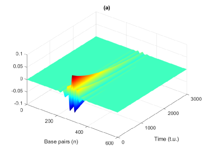
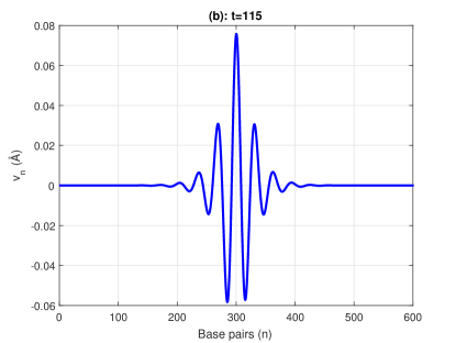
Figure 3: (Color online) (a) Analytical stretching of the nucleotide pair as a function of the time and the number of base pairs. (b) stretching of the nucleotide pair as a function of the number of base pairs at $t=115$ for $s=3.00$, $\varepsilon=0.9$, $u_{e}=1$, $\gamma_{0}=0.15$ $t.u^{-1}$, $u_{c}=0.45u_{e}$ and $q_{n}^{0}r=\frac{\pi}{16}$.

The solution Eq. (43) represents the breather solution in the DNA molecule suggested by the Infrared and Raman experiments [35]. This solution is represented in Figure 3. It can be seen that due to the damping effect, the amplitude of the soliton is a decreasing function of time and hence it will propagates only for a limited distance and vanishes.

Prohofsky et al. have shown in their studies [35] that, the breather can be strongly located, or distributed on a wide zone of the DNA molecule and could be at the origin of the localization of the energy in the molecule which lead to the local denaturation.

It is noteworthy to mention that if one uses the semi-discrete approach [11, 12], the results fails in the derivation of the breather soliton profile Eq. (43). In fact, we can obtain a similar CGL equation Eq. (30), but with a different dispersion coefficient containing continuous derivatives instead of difference operators as given in equation Eq. (28). Using the semi-discrete approach, we obtain:

$$\begin{split}&P_{r}=\frac{1}{2\omega_{r}}\Big{[}\sum\limits_{l=1}\Big{(}\frac{J_{l}}{m}+\omega_{i}\gamma_{l}\Big{)}(rl)^{2}\cos(qlr)-|v_{g\gamma}|^{2}\Big{]},\;\ P_{i}=-\frac{1}{2}\sum\limits_{l=1}\gamma_{l}(rl)^{2}\cos(qrl),\\ &\omega_{r}=\omega\sqrt{1-\Big{(}\frac{\gamma}{2\omega}\Big{)}^{2}},\;\omega^{2}=\omega_{g}^{2}+4\sum\limits_{l=1}\frac{J_{l}}{m}\sin^{2}(qrl/2),\;\ \omega_{i}=-\frac{\gamma}{2},\;\ \gamma=\gamma^{st}+4\sum\limits_{l=1}\gamma_{l}\sin^{2}(qrl/2),\\ &v_{gr}=\frac{r}{\omega_{r}}\sum\limits_{l=1}\Big{(}\frac{J_{l}}{m}+\omega_{i}\gamma_{l}\Big{)}l\sin(qrl),\;\ v_{gi}=-r\sum\limits_{l=1}\gamma_{l}l\sin(qrl),\;\ \varsigma=\omega_{g}^{2}+\frac{4}{m}\sum\limits_{l=1}J_{l}\sin^{2}(qrl),\\ &Q_{r}=-\frac{\omega_{g}^{2}\alpha}{\omega_{r}}(-2\alpha+\frac{3}{2}\beta/\alpha+BC),\;\ Q_{i}=-\frac{\omega_{g}^{2}\alpha}{\omega_{r}}CD_{1}\;\ B=4\omega_{r}^{2}\varsigma,\;\ D_{1}=2\gamma\omega_{r},\;\ C=\frac{\omega_{g}^{2}\alpha}{B^{2}+D_{1}^{2}}.\end{split}$$ (45)

In Eq. (45), the appearance of continuous derivatives can cause a divergence of both the group velocity $v_{g}$ and the dispersion coefficient $P$. The coefficients oscillate for different values of chain length and does not converge to a definite value.

4 Numerical investigations.

The results discussed in the previous section are obtained from the CGL equation (Eq. (30)) derived after some approximations and hypothesis and not from the discrete EOM. In order to verify the analytical predictions and check if the above analytical breather soliton can survive in the discrete lattice, the numerical simulations of the discrete EOM (Eq. (11)) is carried out by means of a standard fourth-order Runge-Kutta computational scheme with periodic boundary conditions. In our simulations we use the initial condition given by Eq. (43) and time step $h=2\pi/N$ $t.u.$ with $N=600$. Figure 4 presents the $3D$ and $2D$ time-evolution of the solution for a value of LRI parameter $s=3.00$, and we observe the decreasing of the amplitude of the soliton due to the damping forces (Figure 4a). Figure 4b presents the aspect of the numerical solution at $t=115$. As predicted by the analytical results, we observe that the breathing mode appears in DNA molecule when the wave vector is small, namely $q_{n}r\leq\frac{\pi}{12}$ which corresponds to the domain where the real parts of the angular frequency is different from zero. In Figure 5 and Figure 6, we have depicted the $2D$ schematic representation of the analytical and numerical solutions at few time positions for two different wave vectors ($q_{n}r=\pi/16$ and $q_{n}r=\pi/18$): $t=0$, $t=50$, $t=200$ and $t=300$. We observe that when the wave vector increases, the width of the soliton grows by increasing the number of base pairs in the bubble. At the same time, the wave amplitude must increase in order to keep the soliton within the lattice length limits. Therefore, small wavenumber leads to a more localized solution. The decreasing of the amplitude of the soliton in time is observed. Also we notice that the shape, the decay of the amplitude and the number of base pairs in the bubble of both solutions after a limited time propagation are the same. But after a long time propagation the number of base pairs which form the bubble remains constant, the shape of the numerical solution is slightly modified also the decay in the amplitude of the numerical solution is less than the theoretical expectations, due to the discreteness effects which usually tend to slow down the motion [10]. These results confirm that our analytical solution is stable and suitable to predict formation of breather solitons in the DNA molecular chain in the presence of damping and LRI forces.

5 Conclusion

In this work, we have studied the dynamics of breather solitons in a long-range version of the Peyrard-Bishop DNA model taking into Stokes and hydrodynamical viscous forces. Using the discrete difference operator technique, we have shown that the out-of-phase motion can be described by the CGL equation. As compared to the semi-discrete approach, this technique can lead to the correct expression for the soliton parameters. The breather soliton which represents the opening of base pairs experimentally observed in the DNA molecular chain in the form of bubble, has been found stable when it propagates, however its amplitude decreases due to damping effect. Our numerical simulations have confirmed the validity of the analytical approximate results.

References

S.W. Englander et al., Proc. Natl. Acad. Sci. U.S.A. 77, 7222 (1980).

S. Yomosa, Phys. Rev. A 27, 2120 (1983).

S. Homma and S. Takeno, Prog. Theor. Phys. 70, 308 (1983);.

S. Takeno and S. Homma, Prog. Theor. Phys. 72, 679 (1984).

M. Peyrard and A.R. Bishop, Phys. Rev. Lett. 62, 2755 (1989).

T. Dauxois, M. Peyrard, and A.R. Bishop, Phys. Rev. E 47, R44 (1993).

T. Dauxois and M. Peyrard, Phys. Rev. E 51, 4027 (1995).

A. Campa and A. Giansanti, Phys. Rev. E 58, 3585 (1998).

T. Dauxois, Phys. Lett. A. l59, 390 (l991).

S. Zdravković and M.V. Satarić, Chin. Phys. Lett. 24, 1210 (2003).

S. Zdravković M.V. Satarić and L. Hadžievski, Chaos 20, 043141 (2010).

C. Calladine et al., Understanding DNA, 3rd edition (Academic Press, London, 2004).

N.N. Shafranovskaya et al., Pis’ma. Zh. Eksp. Teor. Fiz. 15, 404 (1972).

D.C. Rau and V.A. Parsegian, Biophysics J. 61, 246 (1992).

Y. Ishimori, Prog. Theor. Phys. 68, 402 (1982).

Yu. B. Gaididei, S.F. Mingaleev, P.L. Christiansen and K. $\emptyset$. Rasmussen, Phys. Lett. A. 222, 152 (1996).

S. F. Mingaleev, Yu.B. Gaididei, and F.G. Mertens, Phys. Rev. E. 58, 3833 (1998).

A. Mvogo, G.H. Ben-Bolie and T.C. Kofané, Phys. Lett. A. 378, 2509 (2014).

A. Mvogo, G.H. Ben-Bolie and T.C. Kofané, Chaos 25, 063115 (2015).

G. Miloshevich, J.P. Nguenang, T. Dauxois, R. Khomeriki and S. Ruffo, J. Phys. A: Math. Theor. 50, 12LT02 (2017).

N.R. Pereira and L. Stenflo, Phys. Fluids 20, 1733 (1977).

S. Flach, Phys. Rev. E 58, R4116 (1998).

Y.B. Gaididei, S.F. Mingaleev, P.L. Christiansen and K.$\emptyset$ Rasmussen, Phys. Rev. E 55, 6141 (1997).

M. Peyrard, Nonlinearity 17, R1 (2004).

E. Arévalo and F.G. Mertens, Phys. Rev. E. 67, 016610 (2003).

C. Brunhuber and F.G. Mertens, Phys. Rev. E. 73, 016614 (2006).

I. Daumont and M. Peyrard, Chaos 13, 624 (2003).

M. Peyrard and I. Daumont, Europhys. Lett., 59 834 (2002).

E. Arévalo Yu. Gaididei and F.G. Mertens, Eur. Phys. J. B 27, 63 (2002)

J.W. Boyle, S. A. Nikitov, A.D. Boardman, J.G. Booth and K. Booth, Phys. Rev. B 53, 12173 (1996)

L.M. Hocking and K. Stewartson, Proc. R. Soc. London, Ser. A 326, 289 (1972).

N. Akhmediev and A. Ankiewicz: Solitons of the Complex Ginzburg-Landau Equation in Spatial Solitons, Edited by S. Trillo, p. 311 (Springer, New York, 2002).

A.C. Scott, F.Y.F. Chu and D.W. McLaughlin, Proc. IEEE. E. 61, 1443 (1973).

B.F. Putnam, L.L. Van Zandt, E.W. Prohofsky, K.C. Lu, and W. N. Mei, Biophys. J. 35, 271 (1981); E.W. Prohofsky, K.C. Lu, L.L. Van Zandt and B.F. Putnam, Phys. Lett. A 70, 492 (1979).

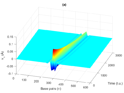
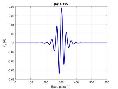
Figure 4: (Color online) (a) Numerical stretching of the nucleotide pair as a function of the time and the number of base pairs. (b) stretching of the nucleotide pair as a function of the number of base pairs at $t=115$ for $s=3.00$, $\varepsilon=0.9$, $u_{e}=1$, $\gamma_{0}=0.15$ $t.u^{-1}$, $u_{c}=0.45u_{e}$ and $q_{n}^{0}r=\frac{\pi}{16}$.

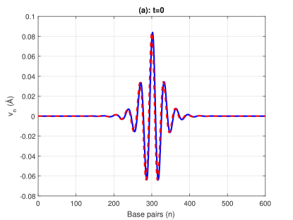
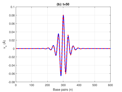
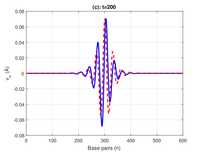
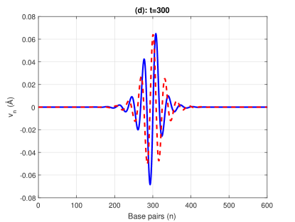
Figure 5: (Color online) Comparison between analytical and numerical solution of the EOM Eq. (11) at different time positions for $s=3.00$, $\varepsilon=0.9$, $u_{e}=1$, $\gamma_{0}=0.15$ $t.u^{-1}$, $u_{c}=0.45u_{e}$ and $q_{n}^{0}r=\frac{\pi}{16}$. (solid blue line) the numerical solution. (dash red line) the analytical solution.

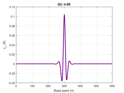
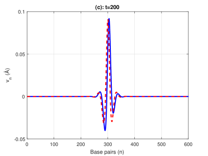
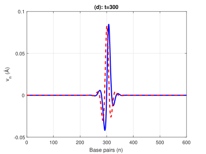
Figure 6: (Color online) Comparison between analytical and numerical solution of the EOM Eq. (11) at different time positions for $s=3.00$, $\varepsilon=0.9$, $u_{e}=1$, $\gamma_{0}=0.15$ $t.u^{-1}$, $u_{c}=0.45u_{e}$ and $q_{n}^{0}r=\frac{\pi}{18}$. (solid blue line) the numerical solution. (dash red line) the analytical solution.