Self-organized criticality in type I X-ray bursts
Abstract
Type I X-ray bursts in a low-mass X-ray binary (LMXB) are caused by unstable nuclear burning of accreted materials. Semi-analytical and numerical studies of unstable nuclear burning have successfully reproduced partial properties of this kind of burst. However, some other properties (e.g. the waiting time) are not well explained. In this paper, we find that the probability distributions of fluence, peak count, rise time, duration and waiting time can be described as power-law-like distributions. This indicates that type I X-ray bursts may be governed by a self-organized criticality (SOC) process. The power-law index of waiting time distribution (WTD) is around , which is not predicted by any current waiting time model. We propose a physical burst rate model, in which the mean occurrence rate is inversely proportional to time . In this case, the WTD is well explained by a non-stationary Poisson process within the SOC theory. In this theory, the burst size is also predicted to follow a power-law distribution, which requires that the emission area possesses only part of the neutron star surface. Furthermore, we find that the WTDs of some astrophysical phenomena can also be described by similar occurrence rate models.
keywords:
accretion, accretion disks – X-ray: bursts – X-rays: binaries – stars: neutron1 Introduction
Type I X-ray bursts or thermonuclear bursts are nuclear shell flashes in low-mass X-ray binary (LMXB) systems. The accreted hydrogen/helium matter accumulates into a thin shell upon the neutron star surface and releases nuclear energy unstably (Woosley & Taam, 1976; Maraschi & Cavaliere, 1977; Joss, 1977). Recently, a class of ‘superburst’ was also found and though to be caused by unstable burning carbon (Strohmayer & Brown, 2002). Thermonuclear bursts were first observed in 1970’s (Grindlay et al., 1976; Belian, Conner, & Evans, 1976). Since then, type I X-ray bursts have been widely studied observationally and theoretically.
This type of bursts offer a chance to probe the properties of neutron stars, such as the mass-radius relation, magnetic field, and spin (Lewin, van Paradijs, & Taam, 1993; Watts, 2012). Theoretical models have been proposed and successfully explain most of burst properties (Joss, 1978; Fujimoto, Hanawa, & Miyaji, 1981; Ayasli & Joss, 1982; Fujimoto et al., 1987; Fushiki & Lamb, 1987; Lewin, van Paradijs, & Taam, 1993; Narayan & Heyl, 2003; Woosley et al., 2004; Fisker, Schatz, & Thielemann, 2008; José et al., 2010), and several ignition regimes have been identified as resulting from different burst fuel compositions and accretion rates (e.g. see Fujimoto, Hanawa, & Miyaji, 1981; Narayan & Heyl, 2003). However, some properties, such as waiting time or recurrence time, have not been fully understood.
For normal bursts (H/He flashes), the theoretical waiting time is , roughly a few hours in LMXBs, where is the critical shell mass when burst can be ignited and is the accretion rate (e.g. see Narayan & Heyl, 2003). Galloway et al. (2004) found that the waiting time for GS 1826-24 is proportional to , assuming that the accretion rate is linearly proportional to the observed X-ray flux. However, this should be not important. Because, for most sources the accretion rate changes only in a small range (e.g. see Table 10 of Galloway et al., 2008). Keek et al. (2010) studied the effect of the data gaps using Monte Carlo simulations. They assumed that the “intrinsic” waiting time distribution of EXO 0748-676 follows a bimodal distribution of mean values at 12.7 minutes and 3.0 hours with 16% widths. Then due to the effect of data gaps, the resulting waiting time will span 2-3 orders of magnitude. But it should be noted that further interpretation is needed that why the “intrinsic” waiting time follows a bimodal distribution. Even though, this still does not cover the observed waiting times well. A detailed study of normal bursts from Rossi X-ray Timing Explorer (RXTE) showed that the waiting times from single source can span 4-5 orders of magnitude, from a few minutes to years (Galloway et al., 2008). In their paper, the ‘superburst’ (carbon flashes) is not taken into consideration. In addition, several challenges to the theoretical models of the waiting time were also noted (Galloway et al., 2008; Keek et al., 2010), including very short waiting-time bursts. Meanwhile, it is not fully understood what causes the asymmetric brightness patches, also known as burst oscillations, which might be related to the emission area of the bursts (Strohmayer et al., 1996; Watts, 2012). Thus further study is needed.
In this paper, we analyze the type I X-ray burst catalog of Galloway et al. (2008) using a statistical method. We focus on the probability distributions of waiting time, burst fluence, peak counts, rise time and duration time. Below, we will explain waiting time distribution (WTD) by a non-stationary Poisson process, where the mean burst rate when . This is quite a bit different with previous understanding of waiting time . Data analysis and results are presented in the next section. In section 3, we extend our model of waiting time distribution. Summary and discussions are presented in section 4.
2 Data analysis and results
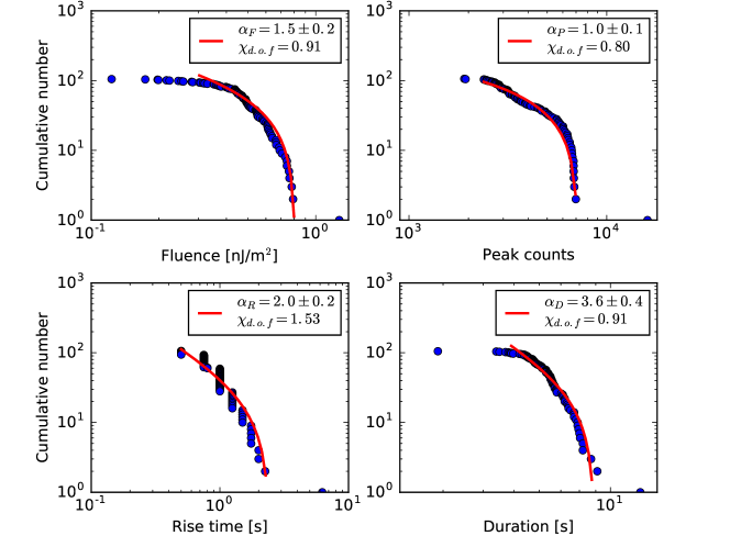
There are three burst cases based on the accretion rates and ignition regimes. The burst property is quite different for them. We give a brief summary of these cases in Table 1. More detailed summary can be seen in Table 1 of Galloway et al. (2008) and references therein. In this paper, we study the catalogue compiled by Galloway et al. (2008). This catalogue contains 1187 burst from 48 accreting neutron stars, while only four of them have around 100 bursts (see Table 4 of Galloway et al., 2008). Therefore, we focus on these four sources and list some properties of them in Table 1. The largest sample, 4U 1636-536, contains 171 bursts. However, this source has both pure He bursts and mixed H and He bursts. Since the burst properties (e.g. peak counts, duration, rise time, and fluence) differ a lot in these two burst cases, we do not choose it as an example for study. Instead, we take the second largest source 4U 1728-34 as an example, which contains only pure He flashes.
Since the burst number of this source is small, we study the cumulative number distribution of the data. If the differential distributions of the fluence, peak counts, rise time and duration time follow the Pareto distributions, i. e. for , the cumulative number would be
| (1) |
where corresponds to observed parameter and its minimum and maximum value are and . is the total number of the sample. The index is the scaling parameter for the distributions, namely, for fluence, for peak counts, for rise time and for duration. It is worth noting that a physical threshold of an instability or the incomplete sampling of small events, which is widely found in astrophysics (Aschwanden, 2015), can cause fluctuations at the left part. Thus we do not take into account this part when fitting. We fit the parameter by minimizing the reduced , which is
| (2) |
where is the number of parameters in the calculation, is the observed cumulative number of events and . The best-fitted values of the scaling parameters and uncertainties are , , and for 4U 1728-34. We show the best-fitted value of the scaling parameters and the minimum in Figure 1. For the pure random noise, the expected is around 1. Using the same method, we find that the other three sources in Table 1 also have similar distributions as 4U 1728-34. We also compare our results with the predicted values of the fractal-diffusive transport self-organized criticality (SOC) model proposed by Aschwanden (2014), which gives , and . The value of and are not well consistent with the model predictions, while shows good agreement. But in fact, the scaling parameters in some astrophysical phenomena have significant deviations from this model (see Table 1 of Aschwanden, 2014, for a good summary). One possible reason is that the sample size is small. For example, the incomplete sampling of small events near the threshold (Aschwanden, 2015) could make a big difference, especially when the observed maximum value in our research.
Based on the criteria proposed by Aschwanden (2011, 2014), which are statistical independence of events, non-linear growth phase, random rise times and power-law distribution of these observed parameters, type I X-ray burst can be explained by a SOC process. The SOC theory predicts that subsystems self-organize owing to some driving force to a critical state, at which a slight perturbation can cause a chain reaction of any size within the system (Bak, Tang, & Wiesenfeld, 1987).
The SOC theory also predicts a power-law distribution of waiting times (Aschwanden, 2011; Marković & Gros, 2014). The WTD has been widely discussed in astrophysics (Wheatland, Sturrock, & McTiernan, 1998; Aschwanden & McTiernan, 2010; Wang & Dai, 2013; Li et al., 2014; Wang et al., 2015; Guidorzi et al., 2015; Wang & Yu, 2017). In the SOC theory, WTD is usually described as a (non-)stationary Poisson process. The probability function is expressed by (Wheatland, Sturrock, & McTiernan, 1998)
| (3) |
where is the waiting time, is the period, and is the burst occurrence rate. Below, we model the occurrence rate .
We propose that the burst rate can be modelled by . The reason is shown below. Type I X-ray bursts are induced by a thin-shell instability. In LMXBs, the accreted H/He fuel accumulates on the stellar surface and forms a shell. The typical time for nuclear energy release is , where is the mass of the shell and is the nuclear energy generation rate (Hōshi, 1968; Joss, 1977). In the quiescent stage, remains almost unchanged. Meanwhile, the energy will be diffused in a typical time , which also depends on the stellar temperature and the opacity of the shell (Hōshi, 1968; Ayasli & Joss, 1982). The condition for triggering a burst is , where the critical shell mass is obtained by (Hōshi, 1968; Ayasli & Joss, 1982). Alternative descriptions of this critical condition are also used (Fujimoto, Hanawa, & Miyaji, 1981; Fujimoto et al., 1987; Narayan & Heyl, 2003). We assume that happens at a typical time . When the shell grows thick enough at a time , any perturbation affects the stellar hydrostatic structure significantly and leads to stable nuclear burning (Schwarzschild & Harm, 1965). Therefore, a burst can be triggered only in a time range . Since these time-scales are mainly determined by the shell mass, it is plausible to assume that the occurrence rate also mainly depends on the shell mass. Because the accreted mass is proportional to time, we can adopt the burst rate as
| (4) |
The occurrence rate is taken as when . We put all the time-dependent effects into the power-law index , which contains the dependence on shell mass and the possible time evolution of accretion rate . The coefficient is a normalization constant, i.e.,
| (5) |
Accordingly, there are three free parameters (, and ) in this model. Substituting the above equation into equation (3), we can obtain the differential probability distribution
| (6) |
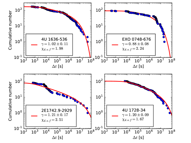
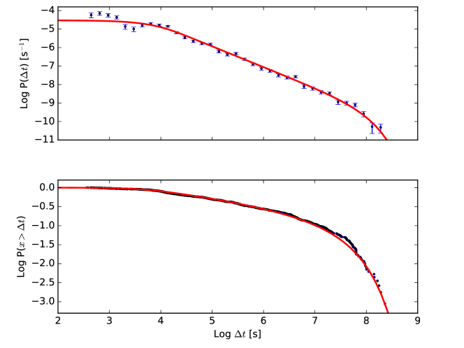
The full catalogue contains 1128 waiting times, calculated in the observer’s frame (Galloway et al., 2008). In this case, the gravitational redshift is important, which is hard to determine for each source. But it seems that for most equations of state in neutron stars, the gravitational redshifts span a relative narrow range (Lattimer & Prakash, 2001). Thus it is plausible to ignore the gravitational redshift effect, especially when we study the WTDs in a single source. Here we study the selected four representative sources as shown in Table 1 and the full sample (1128 waiting times). The cumulative number distributions of four sources are shown in Figure 2. The power-law indices of these four samples are well consistent with each other and the typical value is . We use the above waiting time model to fit the data by the transformation of , where . The best-fitting curves are shown in Figure 2 and the best-fitting parameters are given in Table 1. Then we study the full sample. Since the number of waiting time is large enough, we study both the differential probability distribution and cumulative probability distribution, which are shown in Figure 3. The best-fitting values are , s and s. The value of is well consistent with those of four representative samples. The typical value implies . Analytically, we substitute into equation (5), which gives . After substituting it into equation (6), the probability distribution of occurrence rate is
| (7) |
In general case, the value of is much larger than , i.e., . So the term has a maximum value of at , and varies in the range For typical values of s and s, this range becomes . Thus this part is almost changeless. Then the probability distribution of occurrence rate is approximately , which is consistent with the data. However, the fractal-diffusive transport SOC model proposed by Aschwanden (2014) predicts that . There is no model that predicts a power-law index of WTD.
As shown in Table 1, the time scales and differs a little in four sources, because these time scales depend on the accretion rate and fuel compositions. Theoretically, if the accretion rate and the composition of accreted material are changeless, the time scales and for single sources would be almost constant. Thus, we have almost pure power-law distribution in 4U 1728-34, as shown in Figure 2. If the accretion rate and composition change, these time scales would evolve. So only their mean value can be obtained statistically. Meanwhile, we should keep in mind that the data gaps of RXTE observations could introduce an uncertainty on . The main data gaps originate from the South Atlantic Anomaly and the Earth occultation, which pollute the data with waiting times around satellite period, about s (Keek et al., 2010; Aschwanden & McTiernan, 2010), which is close to .
Since SOC theory is well consistent with the statistical properties of type I X-ray burst, it is plausible to infer that the other ‘SOC parameter’ such as the burst size obeys a power-law-like distribution based on the macroscopic description of SOC systems by Aschwanden (2014). In their model, the power-law-like distributions of peak flux, energy and duration are derived based on the condition that the size of the event follows a power-law-like distribution. Actually, the power-law-like distribution of size have been observed in many astrophysical phenomena, such as lunar craters, asteroid belt, and various solar phenomena (see Aschwanden, 2011, 2014; Aschwanden et al., 2016, and references therein). In the same case, we would also expect that the size (e.g. depth, area, and volume) of type I X-ray bursts obeys a power-law-like distribution. In this case, it is very possible that not all the accreted materiel burns during a burst. Some materiel will remain, and thus it take less time to trigger the next burst. Gottwald et al. (1987) suggested that 10-15 percent of the fuel could remain to the subsequent burst by studying the bursts of EXO 0748-676. But more studied are needed to obtain the amount of unburned material in a burst. Recently, Keek & Heger (2017) found that the short waiting time burst can be explained if some fuel is left unburned during a burst at a shallow depth by using one-dimensional simulations. It is also possible that the emission area is just a part of the surface, such as a hot spot. And such hot spot model is used to explain the burst oscillations (Strohmayer et al., 1996; Watts, 2012). Thus more detailed research for the amount of burst fuel is needed, which is beyond the scope of this paper.
3 Extension of the WTD model
Since we have successfully used this WTD model to explain type I X-ray burst, we further investigate the applicability of this model. Generally, a function is adopted to fit waiting time distribution, where with two parameters of and (Aschwanden, 2011; Li et al., 2014; Guidorzi et al., 2015). The resulting probability function can be expressed as with (equation 8 of Guidorzi et al., 2015). However, this model is phenomenological and only applicable for . We find that the occurrence rate model has a broader application. Making a substitution , equation (6) becomes
| (8) |
which implies . The index might vary in different astrophysical phenomena. Therefore, different power-law indices of WTD are expected. The case of a similar form of has been partially studied (Aschwanden & McTiernan, 2010; Aschwanden, 2011), where the case of corresponds to the stationary Poisson process and for , the corresponding power-law index of WTD is .
The power-law indices of the WTDs in astrophysics (Aschwanden, 2011) or geophysics, such as earthquakes (Bak et al., 2002), are generally in the range . Therefore, these WTDs in different systems, can be understood by the form of by varying or . For examples, the WTD of X-ray solar flares observed by the Hard X-Ray Spectrometer shows a power-law with index (Pearce, Rowe, & Yeung, 1993), which can be hardly explained by previous models. However, our model can explain it by adopting .
4 Summary and discussions
In summary, we have found that the fluence, peak counts, rise time and duration can be described by power-law distributions. This suggests that type I X-ray bursts are governed by a SOC process, which describes a critical state in a non-linear energy dissipation system. For type I X-ray bursts, the critical state is reached at when the nuclear energy generation rate exceeds the diffusion loss rate. Once a burst is triggered, the nuclear energy is released unstably. The WTD is well explained by a non-stationary Poisson process with occurrence rate . Using very similar models, we can also explain the WTDs in other SOC phenomena, such as various solar phenomena and activities in flare stars. Using occurrence rate models with different , we find that the power-law index of waiting time distribution is .
Meanwhile, it’s noteworthy that the burst size would also follow a power-law distribution as predicted by the SOC theory (Bak, Tang, & Wiesenfeld, 1987; Aschwanden, 2014). This implies that only a part of the fuel contributes to the observed burst. Under the circumstance, the burst depth, area, and volume could be different to different bursts. Interestingly, the hot spot model can provide a simple explanation of the burst oscillations, which have been found in many bursts (Strohmayer et al., 1996; Watts, 2012). In addition, the unburned materials could participate in the subsequent burst, if the amount of unburned material is large enough, the waiting time of the subsequent burst could be very short, which is in agreement with a recently study by Keek & Heger (2017) using one-dimension simulations.
Acknowledgements
We have greatly benefited from the on-line catalogue of Galloway et al. (2008). We thank the anonymous referee and Kinwah Wu for useful suggestions. This work is supported by the National Basic Research Program (“973” Program) of China (grant No. 2014CB845800) and National Natural Science Foundation of China (grants 11422325, 11373022, and 11573014), and the Excellent Youth Foundation of Jiangsu Province (BK20140016). JSW is also partially supported by CSC.
| Name | 4U 1636-536 | EXO 0748-676 | 2E 1742.9-2929 | 4U 1728-34 |
| case | case 3 | case 2 | ||
| H&He/He | H&He | H&He | He | |
| s) | ||||
| s) |
References
- Aschwanden (2011) Aschwanden, M. J., Self-Organized Criticality in Astrophysics, 2011, Springer-Verlag: Berlin
- Aschwanden (2014) Aschwanden, M. J. 2014, ApJ, 782, 54
- Aschwanden (2015) Aschwanden, M. J. 2015, ApJ, 814, 19
- Aschwanden & McTiernan (2010) Aschwanden, M. J., McTiernan, J. M. 2010, ApJ, 717, 683
- Aschwanden et al. (2016) Aschwanden, M. J., Crosby, N. B., Dimitropoulou, M., et al. 2016, Space Sci. Rev., 198, 47
- Ayasli & Joss (1982) Ayasli, S., Joss, P. C. 1982, ApJ, 256, 637
- Bak et al. (2002) Bak, P., Christensen, K., Danon, L., & Scanlon, T. 2002, Physical Review Letters, 88, 178501
- Bak, Tang, & Wiesenfeld (1987) Bak, P., Tang, C., Wiesenfeld, K. 1987, Physical Review Letters, 59, 381
- Belian, Conner, & Evans (1976) Belian, R. D., Conner, J. P., Evans, W. D. 1976, ApJ, 206, L135
- Fisker, Schatz, & Thielemann (2008) Fisker, J. L., Schatz, H., Thielemann, F.-K. 2008, ApJS, 174, 261-276
- Fujimoto, Hanawa, & Miyaji (1981) Fujimoto, M. Y., Hanawa, T., Miyaji, S. 1981, ApJ, 247, 267
- Fujimoto et al. (1987) Fujimoto, M. Y., Sztajno, M., Lewin, W. H. G., van Paradijs, J. 1987, ApJ, 319, 902
- Fushiki & Lamb (1987) Fushiki, I., Lamb, D. Q. 1987, ApJ, 323, L55
- Galloway et al. (2004) Galloway, D. K., Cumming, A., Kuulkers, E., et al. 2004, ApJ, 601, 466
- Galloway et al. (2008) Galloway, D. K., Muno, M. P., Hartman, J. M., Psaltis, D., Chakrabarty, D. 2008, ApJS, 179, 360-422
- Gottwald et al. (1987) Gottwald, M., Haberl, F., Parmar, A. N., White, N. E. 1987, ApJ, 323, 575
- Grindlay et al. (1976) Grindlay, J., Gursky, H., Schnopper, H., et al. 1976, ApJ, 205, L127
- Guidorzi et al. (2015) Guidorzi, C., Dichiara, S., Frontera, F., et al. 2015, ApJ, 801, 57
- Hōshi (1968) Hōshi, R. 1968, Progress of Theoretical Physics, 39, 957
- José et al. (2010) José, J., Moreno, F., Parikh, A., Iliadis, C. 2010, ApJS, 189, 204
- Joss (1977) Joss, P. C. 1977, Nature, 270, 310
- Joss (1978) Joss, P. C. 1978, ApJ, 225, L123
- Keek et al. (2010) Keek, L., Galloway, D. K., in’t Zand, J. J. M., Heger, A. 2010, ApJ, 718, 292
- Keek & Heger (2017) Keek L., Heger A., 2017, ApJ, 842, 113
- Lattimer & Prakash (2001) Lattimer, J. M., Prakash, M. 2001, ApJ, 550, 426
- Lewin, van Paradijs, & Taam (1993) Lewin, W. H. G., van Paradijs, J., Taam, R. E. 1993, Space Sci. Rev., 62, 223
- Li et al. (2014) Li, C., Zhong, S. J., Wang, L., Su, W., Fang, C. 2014, ApJ, 792, L26
- Maraschi & Cavaliere (1977) Maraschi, L., Cavaliere, A. 1977, in Highlights in Astronomy, Vol. 4, ed. E. A. Müller (Dordrecht: Reidel), Part 1, 127
- Marković & Gros (2014) Marković, D., Gros, C. 2014, Phys. Rep., 536, 41
- Narayan & Heyl (2003) Narayan, R., Heyl, J. S. 2003, ApJ, 599, 419
- Pearce, Rowe, & Yeung (1993) Pearce, G., Rowe, A. K., Yeung, J. 1993, Ap&SS, 208, 99
- Schwarzschild & Harm (1965) Schwarzschild, M., Harm, R. 1965, ApJ, 142, 855
- Strohmayer & Brown (2002) Strohmayer, T. E., Brown, E. F. 2002, ApJ, 566, 1045
- Strohmayer et al. (1996) Strohmayer, T. E., Zhang, W., Swank, J. H., et al. 1996, ApJ, 469, L9
- Wang & Dai (2013) Wang, F. Y., Dai, Z. G. 2013, Nature Physics, 9, 465
- Wang et al. (2015) Wang, F. Y., Dai, Z. G., Yi, S. X., Xi, S. Q. 2015, ApJS, 216, 8
- Wang & Yu (2017) Wang, F. Y., Yu, H. 2017, JCAP, 03, 023
- Watts (2012) Watts, A. L. 2012, ARA&A, 50, 609
- Wheatland, Sturrock, & McTiernan (1998) Wheatland, M. S., Sturrock, P. A., McTiernan, J. M. 1998, ApJ, 509, 448
- Woosley et al. (2004) Woosley, S. E., Heger, A., Cumming, A., et al. 2004, ApJS, 151, 75
- Woosley & Taam (1976) Woosley, S. E., Taam, R. E. 1976, Nature, 263, 101