Statics and kinematics of frameworks in Euclidean and non-Euclidean geometry

1 Introduction

A bar-and-joint framework is made of rigid bars connected at their ends by universal joints. A framework can be constrained to a plane or allowed to move in space. Rigidity of frameworks is a question of practical importance, and its mathematical study goes back to the 19th century. Plate-and-hinge structures such as polyhedra can be represented by bar-and-joint frameworks through replacement of the hinges by bars and rigidifying the plates with the help of diagonals. Thus, rigidity questions for polyhedra belong to the same domain.

There are two ways to approach the rigidity of a framework: through statics, i. e. ability to respond to exterior loads, and through kinematics, i. e. abscence of deformations. A framework is called statically rigid if every system of forces with zero sum and zero moment can be compensated by stresses in the bars of the framework. A framework is called rigid if it cannot be deformed while keeping the lengths of all bars, and infinitesimally rigid if it cannot be deformed so that the lengths of bars stay constant in the first order. As it turns out, static rigidity is equivalent to the infinitesimal rigidity.

The study of statics has a long history. Systems of forces appear in the textbooks of Poinsot [42] and Möbius [36], and the concept of a line-bound force was one of the motivations for Grassman’s introduction of the exterior algebra of a vector space.

Infinitesimal isometric deformations seem to have appeared first in the context of smooth surfaces, see [12] and references therein. In the first half of the 20th century the interest in the isometric deformations was stimulated by the Weyl problem, which was successfully solved in the 50’s by Nirenberg and Alexandrov and Pogorelov. The Weyl problem motivated Alexandrov’s works on polyhedra, in particular his enhanced version of the Legendre-Cauchy-Dehn rigidity theorem for convex polyhedra. For a survey on rigidity of smooth surfaces see [44, 21, 22, 20], for rigidity of frameworks and polyhedra see [9].

The goal of this article is to present the fundamental notions and results from the rigidity theory of frameworks in the Euclidean space and to extend them to the hyperbolic and spherical geometry. Below we state four main theorems whose proofs are given in the subsequent sections.

Theorem A.

A framework in a Euclidean, spherical, or hyperbolic space has equal numbers of kinematic and static degrees of freedom. In particular, infinitesimal rigidity is equivalent to static rigidity.

By the number of static, respectively kinematic, degrees of freedom we mean the dimension of the vector space of unresolvable loads, respectively non-trivial infnitesimal isometric deformations. See Sections 2 and 3 for definitions and for a proof of Theorem A.

Theorem B (Darboux-Sauer correspondence).

The number of degrees of freedom of a Euclidean framework is a projective invariant. In particular, a framework is infinitesimally rigid if and only if any of its projective images is infinitesimally rigid.

The projective invariance of static rigidity follows from the interpretation of a line-bound vector (a force) in a $d$-dimensional Euclidean space as a bivector in $\mathbb{R}^{d+1}$. Linear transformations of $\mathbb{R}^{d+1}$ preserve static dependencies; at the same time they generate projective transformations of $\mathbb{R}\mathrm{P}^{d}$. See Section 4.1.

Theorem C (Infinitesimal Pogorelov maps).

A hyperbolic or a spherical framework has the same number of kinematic degrees of freedom as its geodesic Euclidean image. In particular, it is infinitesimally rigid if and only if its geodesic Euclidean image is.

By a geodesic Euclidean image of a hyperbolic framework we mean its representation in a Beltrami-Cayley-Klein model. A geodesic Euclidean image of a spherical framework is its projection from the center of the sphere to an affine hyperplane. Every geodesic map of an open region in the hyperbolic or spherical space into the Euclidean space differs from those given above by post-composition with a projective map.

Theorem C is related to Theorem B and is also proved in Section 4.1. In the same section we describe the infinitesimal Pogorelov maps that send the static or kinematic vector spaces of a framework to the corresponding vector spaces of its geodesic image.

While the previous three theorems hold for frameworks of any combinatorics and in the space of any dimension, the last one is specific for frameworks in dimension $2$ whose underlying graph is planar.

Theorem D (Maxwell-Cremona correspondence).

For a framework on the sphere or in the Euclidean or hyperbolic plane based on a planar graph the existence of any of the following objects implies the existence of the other two:

1. A self-stress.

2. A reciprocal diagram.

3. A polyhedral lift.

Definitions of reciprocal diagrams and polyhedral lifts slightly differ in different geometries. Also, the theorem has various versions all of which are presented in Section 5.

The theory of isometric deformations extends to the smooth case in a quite straightforward way (and, as we already mentioned, probably preceded the kinematics of frameworks). Accordingly, there are analogs of Theorems B and C for smooth submanifolds of the Euclidean, hyperbolic or spherical space. In fact, Theorem B was proved by Darboux for smooth surfaces and only later by Sauer for frameworks [45]. Also Theorem C was first proved by Pogorelov in [41, Chapter 5] for smooth surfaces. On the other hand, a theory of statics for smooth surfaces containing an analog of Theorem A is not fully developed or at least not widely known. (See however the dissertation of Lecornu [31].)

Let us set up the notation used throughout the article. In the following, $\mathbb{X}^{d}$ stands for either $\mathbb{E}^{d}$ (Euclidean space) or $\mathbb{S}^{d}$ (spherical space) or $\mathbb{H}^{d}$ (hyperbolic space). We often view them as subsets of the real vector space $\mathbb{R}^{d+1}$:

$$\mathbb{E}^{d} =\{x\in\mathbb{R}^{d+1}\mid x_{0}=1\},$$

$$\mathbb{S}^{d} =\{x\in\mathbb{R}^{d+1}\mid\langle x,x\rangle=1\},$$

$$\mathbb{H}^{d} =\{x\in\mathbb{R}^{d+1}\mid\langle x,x\rangle=-1,x_{0}>0\}.$$

Here in the second line $\langle\cdot,\cdot\rangle$ stands for the Euclidean, and in the third line for the Minkowski scalar product:

$$\langle x,y\rangle=\pm x_{0}y_{0}+x_{1}y_{1}+\cdots+x_{d}y_{d}.$$

Sometimes we also use $\sin_{\mathbb{X}}$ and $\cos_{\mathbb{X}}$ to denote $\sin$ and $\cos$ in the spherical and $\sinh$ and $\cosh$ in the hyperbolic case.

2 Kinematics of frameworks

2.1 Motions

Let $\Gamma$ be a graph; we denote its vertex set by $\Gamma_{0}$ and its edge set by $\Gamma_{1}$. For the vertices of $\Gamma$ we use symbols $i,j$ etc. The edges are unordered pairs of elements of $\Gamma_{0}$, and for brevity we usually write $ij$ instead of $\{i,j\}\in\Gamma_{1}$.

Definition 2.1.

A framework in $\mathbb{X}^{d}$ is a graph $\Gamma$ together with a map

$$p\colon\Gamma_{0}\to\mathbb{X}^{d},\quad i\mapsto p_{i}$$

such that $p_{i}\neq p_{j}$ whenever $\{i,j\}\in\Gamma_{1}$. If $\mathbb{X}=\mathbb{S}$, then we additionally require $p_{i}\neq-p_{j}$ for all $\{i,j\}\in\Gamma_{1}$.

This is a mathematical abstraction of a bar-and-joint framework, see the introduction. Note that we allow intersections between the edges.

In a framework $(\Gamma,p)$, every edge receives a non-zero length $\operatorname{dist}(p_{i},p_{j})$. Two frameworks $(\Gamma,p)$ and $(\Gamma,p^{\prime})$ with the same graph are called isometric, if they have the same edge lengths: $\operatorname{dist}(p_{i},p_{j})=\operatorname{dist}(p^{\prime}_{i},p^{\prime}_{j})\text{ for all }\{i,j\}\in\Gamma_{1}.$ Frameworks with the same graph are called congruent, if there is an ambient isometry $\Phi\in\operatorname{Isom}(\mathbb{X}^{d})$ such that $p^{\prime}_{i}=\Phi(p_{i})$ for all $i\in\Gamma_{0}$.

Definition 2.2.

A framework $(\Gamma,p)$ is called globally rigid, if every framework isometric to $(\Gamma,p)$ is also congruent to it.

An isometric deformation of a framework $(\Gamma,p)$ is a continuous family of frameworks $(\Gamma,p(t))$ (i. e. every $p_{i}(t)$ is a continuous path in $\mathbb{X}^{d}$), where $t\in(-\epsilon,\epsilon)$ and $p(0)=p$. An isometric deformation is called trivial, if it is generated by a family of ambient isometries: $p_{i}(t)=\Phi_{t}(p_{i})$.

Definition 2.3.

A framework $(\Gamma,p)$ is called rigid (or locally rigid), if it has no non-trivial isometric deformations. A non-rigid framework is also called flexible.

Clearly, global rigidity implies rigidity, but not vice versa. See Figure 1.

Figure 1: Frameworks in the plane. Left: globally rigid. Middle: rigid but not globally rigid. Right: flexible.

2.2 Infinitesimal motions

Definition 2.4.

A vector field on a framework $(\Gamma,p)$ is a map

$$q\colon\Gamma_{0}\to T\mathbb{X}^{d},\quad i\mapsto q_{i}$$

such that $q_{i}\in T_{p_{i}}\mathbb{X}^{d}$ for all $i$. A vector field is called an infinitesimal isometric deformation of $(\Gamma,p)$, if for some (and hence for every) smooth family of frameworks $(\Gamma,p(t))$ such that

$$p(0)=p,\quad\left.\frac{d}{dt}\right|_{t=0}p_{i}(t)=q_{i}\text{ for all }i\in\Gamma_{0}$$

we have

$$\left.\frac{d}{dt}\right|_{t=0}\operatorname{dist}(p_{i}(t),p_{j}(t))=0$$

for all $\{i,j\}\in\Gamma_{1}$.

Clearly, the infinitesimal isometry condition is equivalent to

$$\langle q_{i},e_{ij}\rangle-\langle q_{j},e_{ji}\rangle=0,$$ (1)

where $e_{ij}\in T_{p_{i}}\mathbb{X}^{d}$ is such that $\exp_{p_{i}}(e_{ij})=p_{j}$. We will rewrite this in a different way.

Lemma 2.5.

A vector field $q$ is an infinitesimal isometric deformation of a framework $(\Gamma,p)$ if and only if

$$\langle p_{i}-p_{j},q_{i}-q_{j}\rangle=0 \text{ in }\mathbb{E}^{d};$$

$$\langle p_{i},q_{j}\rangle+\langle q_{i},p_{j}\rangle=0 \text{ in }\mathbb{S}^{d}\text{ or }\mathbb{H}^{d}.$$

Here $\langle p_{i},q_{j}\rangle$ means the Euclidean, respectively Minkowski scalar product in $\mathbb{R}^{d+1}$, which makes sense if we identify $T_{p_{i}}\mathbb{X}^{d}$ with a linear subspace of $\mathbb{R}^{d+1}$.

Proof.

This follows from (1) and

$$e_{ij}=\begin{cases}\frac{p_{j}-p_{i}}{\|p_{j}-p_{i}\|}&\text{ in }\mathbb{E}^{d};\\ \frac{p_{j}-\langle p_{i},p_{j}\rangle p_{i}}{\sin_{\mathbb{X}}\operatorname{dist}(p_{i},p_{j})}&\text{ in }\mathbb{S}^{d}\text{ and }\mathbb{H}^{d}.\end{cases}$$

∎

An infinitesimal isometric deformation is called trivial, if there is a Killing field $K$ on $\mathbb{X}^{d}$ such that $q_{i}=K(p_{i})$ for all $i$.

Definition 2.6.

A framework $(\Gamma,p)$ is called infinitesimally rigid, if it has no non-trivial infinitesimal isometric deformations.

Theorem 2.7.

An infinitesimally rigid framework is rigid.

For a proof, see [19, 2, 8].

The converse of Theorem 2.7 is false, see Figure 2.

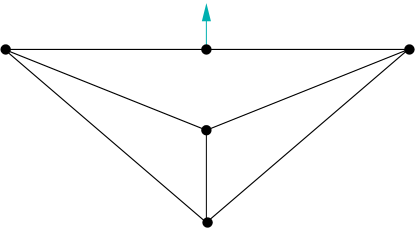
Figure 2: A rigid but infinitesimally flexible framework.

Similarly to the example on Figure 2, one can construct a non-trivial infinitesimal isometric deformation for every framework contained in a geodesic subspace of $\mathbb{X}^{d}$ (provided that the framework has at least $3$ vertices). This is one of the reasons why it is convenient to consider only spanning frameworks: those whose vertices are not contained in a geodesic subspace.

Denote the set of all infinitesimal isometric deformations of a framework $(\Gamma,p)$ by $V(\Gamma,p)$. Due to Lemma 2.5, $V(\Gamma,p)$ is a vector space. The set of trivial infinitesimal isometric deformations is also a vector space; we denote it by $V_{0}(\Gamma,p)$. If $(\Gamma,p)$ is spanning, then $\dim V_{0}(\Gamma,p)=\frac{d(d+1)}{2}$.

Definition 2.8.

The dimension of the quotient space $V(\Gamma,p)/V_{0}(\Gamma,p)$ is called the number of kinematic degrees of freedom of a framework $(\Gamma,p)$.

In particular, infinitesimally rigid frameworks are those with zero kinematic degrees of freedom.

Remark 2.9.

Determining whether a framework is flexible is more difficult than determining whether it is infinitesimally flexible: the latter is a linear problem, the former is an algebraic one. Examples of Bricard octahedra and Kokotsakis polyhedra in Section 2.7 illustrate this.

2.3 Point-line frameworks

A point-line framework in $\mathbb{R}^{2}$ associates to every vertex $i$ of $\Gamma$ either a point $p_{i}$ or a line $l_{i}$ in $\mathbb{R}^{2}$. The edges of $\Gamma$ correspond to the constraints of the form

$$\operatorname{dist}(p_{i},p_{j})=\operatorname{dist}(p^{\prime}_{i},p^{\prime}_{j}),\,\operatorname{dist}(p_{i},l_{j})=\operatorname{dist}(p^{\prime}_{i},l^{\prime}_{j}),\,\angle(l_{i},l_{j})=\angle(l^{\prime}_{i},l^{\prime}_{j}).$$ (2)

For recent works on point-line frameworks see [27, 15].

In the spherical geometry, a point-line framework is equivalent to a standard framework. If we replace every great circle by one of its poles, then the last two constraints in (2) take the form of the first one.

In the hyperbolic geometry, the pole of a line is a point in the de Sitter plane (the complement of the disk in the projective model of $\mathbb{H}^{2}$). Therefore the study of point-line frameworks in $\mathbb{H}^{2}$ can be reduced to the study of standard frameworks in the hyperbolic-de Sitter plane. Moreover, we can allow ideal points, which means assigning horocycles to some of the vertices of $\Gamma$ and fixing the point-horocycle, line-horocycle and horocycle-horocycle distances.

2.4 Constraints counting

One can estimate the dimension of the space of non-congruent realizations of a framework by counting the constraints. If $|\Gamma_{0}|=n$ and $|\Gamma_{1}|=m$, then there are $m$ equations on $dn$ vertex coordinates. Besides, one has to subtract the dimension of the space of trivial motions, which is $\frac{d(d+1)}{2}$ for spanning frameworks. Thus, generically a framework in $\mathbb{X}^{d}$ with $n$ vertices and $m$ edges has $dn-m-\frac{d(d+1)}{2}$ degrees of freedom.

Of course, the above arithmetics does not make much sense without the combinatorics (we can put a lot of edges on a subset of the vertices, allowing the other vertices to fly away). Laman [30] has shown that in dimension $2$ the arithmetics and combinatorics suffice to characterize the generic rigidity. A graph $\Gamma$ is called a Laman graph if $|\Gamma_{1}|=2|\Gamma_{0}|-3$ and every induced subgraph of $\Gamma$ with $k$ vertices has at most $2k-3$ edges.

Theorem 2.10.

A Laman graph is generically rigid, that is the framework $(\Gamma,p)$ is rigid for almost all $p$.

No analog of the Laman condition is known for frameworks in higher dimensions. See [10] for more details on the generic rigidity.

If all faces of a $3$-dimensional polyhedron homeomorphic to a ball are triangles, then its graph satisfies $|\Gamma_{1}|=3|\Gamma_{0}|-6$, that is the above count gives $0$ as the upper bound for degrees of freedom. Rigidity of polyhedra is discussed in the next section.

2.5 Frameworks and polyhedra

One may try to generalize bar-and-joint frameworks by introducing panel-and-hinge structures: rigid polygons sharing pairs of sides and allowed to freely rotate around these sides, or even more generally $n$-dimensional “panels” rotating around $(n-1)$-dimensional “hinges”. A mathematical model for such an object is called a polyhedron or a polyhedral complex. However, there is a way to replace a polyhedral complex by a framework without changing its isometric deformations (global as well as local and infinitesimal). For this, replace every panel by a complete graph on its vertex set. This “rigidifies” the panels and leaves them the freedom to rotate around the hinges.

A particular class of polyhedral complexes are convex polyhedra. According to the Legendre-Cauchy theorem [32, 7], a convex polyhedron is globally rigid among convex polyhedra. There are simple examples of convex polyhedra isometric to non-convex ones. By the Dehn theorem [14] (that can also be proved by the Legendre-Cauchy argument), convex $3$-dimensional polyhedra are infinitesimally rigid.

The Legendre-Cauchy argument applies to spherical and hyperbolic convex polyhedra as well. This allows to prove the rigidity of convex polyhedra in $\mathbb{X}^{d}$ for $d>3$ by induction: the link of a vertex of a $d$-dimensional convex polyhedron is a $(d-1)$-dimensional spherical polyhedron, and the rigidity of links implies the rigidity of the polyhedron.

A simplicial polyhedron (that is one all of whose faces are simplices) has the same kinematic properties as its $1$-skeleton. In a convex non-simplicial polyhedron we can replace every face by a complete graph as described in the first paragraph; but in fact a much “lighter” framework is enough to keep the polyhedron rigid. It suffices to triangulate every $2$-dimensional face in an arbitrary way (without adding new vertices in the interior of the face, vertices on the edges are all right). Again, the Legendre-Cauchy argument ensures the rigidity of all $3$-dimensional faces, and the induction applies as in the previous paragraph, [1, Chapter 10], [52].

As already indicated, the cone over a framework in $\mathbb{S}^{d}$ can be viewed as a panel structure (or a framework) in $\mathbb{E}^{d+1}$. Similarly, a framework in $\mathbb{H}^{d}$ leads to a framework in the $(d+1)$-dimensional Minkowski space.

2.6 Averaging and deaveraging

There is an elegant relation between the infinitesimal and global flexibility. (For smooth surfaces, this idea goes back to the 19th century.)

Theorem 2.11.

1. (Deaveraging.) Let $(\Gamma,p)$ be a framework in $\mathbb{X}^{d}$ with a non-trivial infinitesimal isometric deformation $q$. Define two new frameworks $(\Gamma,p^{+})$ and $(\Gamma,p^{-})$ as follows.

   $$p_{i}^{+}=p_{i}+q_{i},\quad p_{i}^{-}=p_{i}-q_{i} \text{ for }\mathbb{X}=\mathbb{E},$$

   $$p_{i}^{+}=\frac{p_{i}+q_{i}}{\|p_{i}+q_{i}\|},\quad p_{i}^{-}=\frac{p_{i}-q_{i}}{\|p_{i}-q_{i}\|} \text{ for }\mathbb{X}=\mathbb{S}\text{ or }\mathbb{H}.$$

   Then the frameworks $(\Gamma,p^{+})$ and $(\Gamma,p^{-})$ are isometric, but not congruent.

2. (Averaging.) Let $(\Gamma,p^{\prime})$ and $(\Gamma,p^{\prime\prime})$ be two isometric non-congruent frameworks in $\mathbb{X}^{d}$. Put

   $$p_{i}=\frac{p^{\prime}_{i}+p^{\prime\prime}_{i}}{2},\quad q_{i}=\frac{p^{\prime}_{i}-p^{\prime\prime}_{i}}{2} \text{ for }\mathbb{X}=\mathbb{E},$$

   $$p_{i}=\frac{p^{\prime}_{i}+p^{\prime\prime}_{i}}{\|p^{\prime}_{i}+p^{\prime\prime}_{i}\|},\quad q_{i}=\frac{p^{\prime}_{i}-p^{\prime\prime}_{i}}{\|p^{\prime}_{i}+p^{\prime\prime}_{i}\|} \text{ for }\mathbb{X}=\mathbb{S}\text{ or }\mathbb{H}.$$

   Then $q$ is a non-trivial infinitesimal isometric deformation of $(\Gamma,p)$.

In the deaveraging procedure it might happen that $p_{i}^{+}=p_{j}^{+}$ for some $\{i,j\}\in\Gamma_{1}$, so that $p^{+}$ is not a framework. To avoid this, one can replace $q$ by $cq$ for a generic $c\in\mathbb{R}$.

Proof.

Formulas of the averaging are inverse to those of the deaveraging, and both statements can be proved by a direct calculation. Use that in the spherical and the hyperbolic cases we have $\|p_{i}+q_{i}\|=\|p_{i}-q_{i}\|$ due to $\langle p_{i},q_{i}\rangle=0$. Also $q$ is non-trivial if and only if it changes the distance in the first order between some $p_{i}$ and $p_{j}$ not connected by an edge. One can check that this is equivalent to $\operatorname{dist}(p_{i}^{+},p_{j}^{+})\neq\operatorname{dist}(p_{i}^{-},p_{j}^{-})$. ∎

2.7 Examples

In Section 2.4 we spoke about generically rigid graphs. The most interesting examples of flexible frameworks are special realizations of generically rigid graphs.

Example 2.12.

[A planar framework with $9$ edges on $6$ vertices] The frameworks on Figure 3 (which are combinatorially equivalent) are infinitesimally flexible if and only if the lines $a$, $b$, $c$ are concurrent, that is meeting at a point or parallel. This can be proved with the help of the Maxwell-Cremona correspondence, see Example 5.4.

Figure 3: Infinitesimally flexible frameworks in the plane.

Example 2.13 (Another planar framework with $9$ edges on $6$ vertices).

A framework based on the bipartite graph $K_{3,3}$ is infinitesimally flexible if and only if its vertices lie on a (possibly degenerate) conic, see Figure 4. For a proof see [5, 51]. On the left hand side the vertices lie on a circle; the arrows indicate a non-trivial infinitesimal isometric deformation.

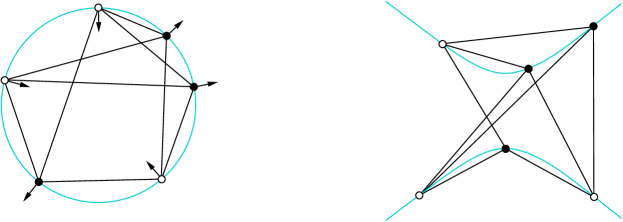
Figure 4: Infinitesimally flexible frameworks in the plane.

The conditions in the above two examples are projectively invariant. Besides, the same criteria hold for frameworks on the sphere or in the projective plane. (Three lines in $\mathbb{H}^{2}$ are called concurrent if they meet at a hyperbolic, ideal, or de Sitter point.) A non-Euclidean conic is one that is depicted by an affine conic in a geodesic model of $\mathbb{S}^{2}$ or $\mathbb{H}^{2}$, see [23].

Example 2.14 (Bricard’s octahedra and Gaifullin’s cross-polytopes).

Flexible octahedra (with intersecting faces) were discovered and classified by Bricard [6], see also [49, 38]. A higher-dimensional analog of the octahedron is called cross-polytope. Recently, flexible cross-polytopes in $\mathbb{X}^{d}$ were classified by Gaifullin [18].

Example 2.15 (Infinitesimally flexible octahedra).

While the description and classification of flexible octahedra requires quite some work, infinitesimally flexible octahedra can be described in a simple and elegant way.

Color the faces of an octahedron white and black so that adjacent faces receive different colors. An octahedron is infinitesimally flexible if and only if the planes of its four white faces meet at a point (which may lie at infinity). As a consequence, the planes of the white faces meet if and only if those of the black faces do.

This theorem was proved independently by Blaschke and Liebmann [4, 33]. The configuration is related to the so called Möbius tetrahedra: a pair of mutually inscribed tetrahedra, [37].

Figure 5 shows two examples of infinitesimally flexible octahedra. The one on the left is a special case of the Schoenhardt octahedron [47]; its bases are regular triangles, and the orthogonal projection of one base to the other makes the triangles concentric with pairwise perpendicular edges.

Figure 5: Infinitesimally flexible octahedra. On the right, the points $A$, $B$, $C$, $D$ must be coplanar.

Theorem B implies that infinitesimally flexible octahedra in $\mathbb{S}^{3}$ and $\mathbb{H}^{3}$ are characterized by the same criterion as those in $\mathbb{E}^{3}$. In the hyperbolic space, the intersection point of four planes may be ideal or hyperideal. In fact, even the vertices of an octahedron may be ideal or hyperideal. Infinitesimally flexible hyperbolic octahedra were used in [25] to construct simple examples of infinitesimally flexible hyperbolic cone-manifolds.

Example 2.16 (Jessen’s icosahedron and its relatives).

In the $xy$-plane of $\mathbb{R}^{3}$, take the rectangle with vertices $(\pm 1,\pm,t,0)$, where $0<t<1$. Take two other rectangles, obtained from this one by $120^{\circ}$ and $240^{\circ}$ rotations around the $x=y=z$ line (which results in cyclic permutations of the coordinates). The convex hull of the twelve vertices of these rectangles is an icosahedron (a regular one for $t=\frac{\sqrt{5}-1}{2}$). Among the edges of this icosahedron are the short sides of the rectangles.

Modify the $1$-skeleton by removing the short sides of rectangles (like the one joining $(1,t,0)$ with $(1,-t,0)$) and inserting the long sides (like the one joining $(1,t,0)$ with $(-1,t,0)$). The resulting framework $p(t)$ is the $1$-skeleton of a non-convex icosahedron. Jessen [28] gave the $t=\frac{1}{2}$ non-convex icosahedron as an example of a closed polyhedron with orthogonal pairs of adjacent faces, but different from the cube. See Figure 6.

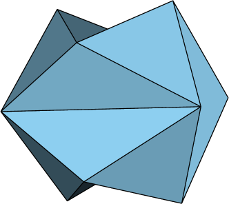
Figure 6: Jessen’s orthogonal and infinitesimally flexible icosahedron.

The framework $p(t)$ has two sorts of edges: the long sides of the rectangles, which have length $2$, and the sides of eight equilateral triangles, which have length $\sqrt{2(t^{2}-t+1)}$. It follows that the frameworks $p(t)$ and $p(1-t)$ are isometric. Note that $p(0)$ collapses to an octahedron: the map $p(t)\colon\Gamma_{0}\to\mathbb{R}^{3}$ sends the vertices of the icosahedral graph to the vertices of a regular octahedron by identifying them in pairs; there are three pairs of edges that are mapped to three diagonals of the octahedron. At the same time, $p(1)$ is the graph of the cuboctahedron with square faces subdivided in a certain way.

Since the average of $p(t)$ and $p(1-t)$ (in the sense of Section 2.6) is $p(\frac{1}{2})$, it follows that Jessen’s icosahedron is infinitesimally flexible.

Theorem B implies that there are spherical and hyperbolic analogs of this construction.

Example 2.17 (Kokotsakis polyhedra).

A Kokotsakis polyhedron with an $n$-gonal base is a panel structure made of a rigid $n$-gon, and $n$ quadrilaterals attached to its edges, and $n$ triangles attached between the quadrilaterals, see Figure 7, left. Generically, a Kokotsakis polyhedron is rigid; it is flexible for certain symmetric configurations, see Figure 7, right.

         

Figure 7: Kokotsakis polyhedra.

Especially interesting are the polyhedra with a quadrangular base, because of their relation to quad-surfaces (polyhedral surfaces made of quadrilaterals with four quadrilaterals around each vertex). A quad-surface is (infinitesimally) flexible if and only if all Kokotsakis polyhedra around its faces are. A famous example of a flexible quad-surface is the Miura-ori [39].

A characterization of infinitesimally flexible Kokotsakis polyhedra was given by Kokotsakis in [29], several flexible examples were constructed in [46, 29]. A complete classification of flexible polyhedra with a quadrangular base is given in [26].

3 Statics of frameworks

3.1 Euclidean statics

In the statics of a rigid body, a force is represented as a line-bound vector: moving the force vector along the line it spans does not change its action on a rigid body.

Definition 3.1.

A force in a Euclidean space is a pair $(p,f)$ with $p\in\mathbb{E}^{d}$, $f\in\mathbb{R}^{d}$. A system of forces is a formal sum $\sum_{i}(p_{i},f_{i})$ that may be transformed according to the following rules:

1. a force with a zero vector is a zero force:

   $$(p,0)\sim 0;$$

2. forces at the same point can be added and scaled as usual:

   $$\lambda_{1}(p,f_{1})+\lambda_{2}(p,f_{2})\sim(p,\lambda_{1}f_{1}+\lambda_{2}f_{2});$$

3. a force may be moved along its line of action:

   $$(p,f)\sim(p+\lambda f,f).$$

One may check from this definition that systems of forces form a vector space of dimension $\frac{d(d+1)}{2}$.

In $\mathbb{E}^{2}$, any system of forces is equivalent either to a single force or to a so called “force couple” $(p_{1},f)+(p_{2},-f)$, where the vector $f$ is not parallel to the line through $p_{1}$ and $p_{2}$.

Definition 3.2.

A load on a Euclidean framework $(\Gamma,p)$ is a map

$$\begin{array}[]{rrcl}f\colon&\Gamma_{0}&\to&\mathbb{R}^{d},\\ &i&\mapsto&f_{i}.\end{array}$$

A load is called an equilibrium load if the system of forces $\sum_{i\in\Gamma_{0}}(p_{i},f_{i})$ is equivalent to a zero force.

A rigid body responds to an equilibrium load by interior stresses that cancel the forces of the load. This motivates the following definition.

Definition 3.3.

A stress on a framework $(\Gamma,p)$ is a map

$$\begin{array}[]{rrcl}w\colon&\Gamma_{1}&\to&\mathbb{R},\\ &ij&\mapsto&w_{ij}=w_{ji}.\end{array}$$

The stress $w$ is said to resolve the load $f$ if

$$f_{i}=\sum_{j\in\Gamma_{0}}w_{ij}(p_{j}-p_{i})\mbox{ for all }i\in\Gamma_{0},$$ (3)

where we put $w_{ij}=0$ for all $ij\notin\Gamma_{1}$.

We denote the vector space of equilibrium loads by $F(\Gamma,p)$, and the vector space of resolvable loads by $F_{0}(\Gamma,p)$. It is easy to see that every resolvable load is an equilibrium load: $F_{0}(\Gamma,p)\subset F(\Gamma,p)$.

Definition 3.4.

The dimension of the quotient space $F(\Gamma,p)/F_{0}(\Gamma,p)$ is called the number of static degrees of freedom of the framework $(\Gamma,p)$.

The framework $(\Gamma,p)$ is called statically rigid if it has zero static degrees of freedom, i. e. if every equilibrium load can be resolved.

3.2 Non-euclidean statics

Definition 3.5.

Let $\mathbb{X}^{d}=\mathbb{S}^{d}$ or $\mathbb{H}^{d}$. A force in $\mathbb{X}^{d}$ is an element of the tangent bundle $T\mathbb{X}^{d}$. We write it as a pair $(p,f)$ with $p\in\mathbb{X}^{d}$ and $f\in T_{p}\mathbb{X}^{d}$.

A system of forces is a formal sum of forces that may be transformed according to the rules of Definition 3.1, where the formula in the rule 2) is replaced by $(p,f)\sim(\exp_{p}(\lambda f),\tau(f))$ with $\tau(f)$ being the result of the parallel transport of $f$ along the geodesic from $p$ to $\exp_{p}(\lambda f)$.

A system of forces on $\mathbb{S}^{2}$ is always equivalent to a single force; a system of forces on $\mathbb{H}^{2}$ is equivalent to either a single force, or an ideal force couple or a hyperideal force couple.

Definition 3.6.

A load on a framework $(\Gamma,p)$ in $\mathbb{X}^{d}$ is a map

$$f\colon\Gamma_{0}\to T\mathbb{X}^{d},\quad f_{i}\in T_{p_{i}}\mathbb{X}^{d}.$$

A load is called an equilibrium load if the system of forces $\sum_{i\in\Gamma_{0}}(p_{i},f_{i})$ is equivalent to a zero force.

In the above definitions, $\mathbb{X}^{d}$ can also stand for $\mathbb{E}^{d}$. The canonical isomorphisms $T_{x}\mathbb{E}^{d}\cong\mathbb{R}^{d}$ result in simplified formulations given in the preceding section.

As in the Euclidean case, a stress on a framework in $\mathbb{X}^{d}$ is a map $w\colon\Gamma_{1}\to\mathbb{R}$. A stress $w$ resolves a load $f$ if

$$f_{i}=\sum_{j\in\Gamma_{0}}w_{ij}\operatorname{dist}(p_{i},p_{j})e_{ij},$$

where $e_{ij}\in T_{p_{i}}\mathbb{X}^{d}$ is such that $\exp_{p_{i}}(e_{ij})=p_{j}$. The following lemma gives an alternative description of the stress resolution.

Lemma 3.7.

A stress $w$ resolves a load $f$ on a framework $(\Gamma,p)$ in $\mathbb{X}^{d}=\mathbb{S}^{d}$ or $\mathbb{H}^{d}$ if and only if for every $i\in\Gamma_{0}$ we have

$$f_{i}-\sum_{j\in\Gamma_{0}}\lambda_{ij}p_{j}\parallel p_{i},$$

where $\lambda_{ij}=w_{ij}\frac{\operatorname{dist}(p_{i},p_{j})}{\sin_{\mathbb{X}}\operatorname{dist}(p_{i},p_{j})}$. Here $f_{i},p_{i}\in\mathbb{R}^{d+1}$ via $\mathbb{X}^{d}\subset\mathbb{R}^{d+1}$.

Proof.

Follows from the identity

$$p_{j}-\cos_{\mathbb{X}}\operatorname{dist}(p_{i},p_{j})p_{i}=p_{j}-\langle p_{i},p_{j}\rangle p_{i}=\sin_{\mathbb{X}}\operatorname{dist}(p_{i},p_{j})\cdot e_{ij}.$$

∎

3.3 Equivalence of static and infinitesimal rigidity

Define a pairing between vector fields and loads on a framework $(\Gamma,p)$:

$$\langle q,f\rangle=\sum_{i\in\Gamma_{0}}\langle q_{i},f_{i}\rangle.$$ (4)

This pairing is non-degenerate and therefore induces a duality between the space of vector fields and the space of loads.

Lemma 3.8 (Principles of virtual work).

Under the pairing (4),

1. the space of infinitesimal motions is the annihilator of the space of resolvable loads:

   $$V(\Gamma,p)=F_{0}(\Gamma,p)^{\circ};$$

2. the space of trivial infinitesimal motions is the annihilator of the space of equilibrium loads:

   $$V_{0}(\Gamma,p)=F(\Gamma,p)^{\circ}.$$

A proof in the Euclidean case can be found in [24]; it transfers to the spherical and the hypebolic cases.

As a consequence, the pairing (4) induces an isomorphism

$$V(\Gamma,p)/V_{0}(\Gamma,p)\cong\left(F(\Gamma,p)/F_{0}(\Gamma,p)\right)^{*}$$ (5)

which implies Theorem A.

The statics of a Euclidean framework is formulated in purely linear terms: loads and stresses on a framework correspond to loads and stresses on its affine image. Together with Theorem A this leads to the following conclusion, which is a special case of Theorem B.

Corollary 3.9.

The number of kinematic degrees of freedom of a Euclidean framework is an affine invariant. In particular, an affine image of an infinitesimally rigid framework is infinitesimally rigid.

Definition 3.10.

The rigidity matrix of a Euclidean framework $(\Gamma,p)$ is a $\Gamma_{1}\times\Gamma_{0}$ matrix with vector entries:

$$\mathcal{R}(\Gamma,p)=\;\scriptstyle{ij}\stackrel{{\scriptstyle\scriptstyle{i}}}{{\left(\begin{array}[]{ccc}&\vdots&\\ \cdots&p_{i}-p_{j}&\cdots\\ &\vdots&\end{array}\right)}}.$$

It has the pattern of the edge-vertex incidence matrix of the graph $\Gamma$, with $p_{i}-p_{j}$ on the intersection of the row $ij$ and the column $i$.

The rows of $\mathcal{R}(\Gamma,p)$ span the space $F_{0}(\Gamma,p)$. The following proposition is a reformulation of the first principle of virtual work.

Lemma 3.11.

Consider $\mathcal{R}(\Gamma,p)$ as the matrix of a map $(\mathbb{R}^{d})^{\Gamma_{0}}\to\mathbb{R}^{\Gamma_{1}}$. Then the following holds:

$$\begin{array}[]{lcl}\ker\mathcal{R}(\Gamma,p)&=&V(\Gamma,p);\\ \operatorname{im}\mathcal{R}(\Gamma,p)^{\top}&=&F_{0}(\Gamma,p).\end{array}$$

Corollary 3.12.

A framework $(\Gamma,p)$ is infinitesimally rigid if and only if

$$\operatorname{rk}\mathcal{R}(\Gamma,p)=d\,|\Gamma_{0}|-\binom{d+1}{2}.$$

4 Projective statics and kinematics

4.1 Projective statics

For $\mathbb{X}^{d}=\mathbb{E}^{d}$, $\mathbb{S}^{d}$ or $\mathbb{H}^{d}$ associate to a force $(p,f)$ in $\mathbb{X}^{d}$ a bivector in $\mathbb{R}^{d+1}$:

$$(p,f)\mapsto p\wedge f.$$ (6)

We use the canonical embeddings $\mathbb{X}^{d}\subset\mathbb{R}^{d+1}$ that allow to view a point $p$ and a vector $f$ as vectors in $\mathbb{R}^{d+1}$.

Lemma 4.1.

The map (6) extends to an isomorphism between the space of systems of forces on $\mathbb{X}^{d}$ and the second exterior power $\Lambda^{2}(\mathbb{R}^{d+1})$.

The equivalence relations from Definition 3.1 ensure that a linear extension is well-defined. For a proof of its bijectivity, see [24].

The above observation motivates the following definitions.

Definition 4.2.

A projective framework is a graph $\Gamma$ together with a map

$$\pi\colon\Gamma_{0}\to\mathbb{R}\mathrm{P}^{d},\quad i\mapsto\pi_{i},$$

such that $\pi_{i}\neq\pi_{j}$ for $ij\in\Gamma_{1}$.

We say that $\phi\in\Lambda^{2}(\mathbb{R}^{d+1})$ is divisible by a vector $v$, if $\phi=v\wedge w$ for some vector $w$. Similarly, we say that $\phi$ is divisible by $\pi\in\mathbb{R}\mathrm{P}^{d}$, if $\phi$ is divisible by a representative of $\pi$.

Definition 4.3.

A load on a projective framework $(\Gamma,\pi)$ is a map

$$\phi\colon\Gamma_{0}\to\Lambda^{2}(\mathbb{R}^{d+1}),\quad i\mapsto\phi_{i},$$

that sends every vertex $i$ to a bivector divisible by $\pi_{i}$. An equilibrium load is one that satisfies

$$\sum_{i\in\Gamma_{0}}\phi_{i}=0.$$

Definition 4.4.

Denote by $\Gamma_{1}^{\mathrm{or}}$ the set of oriented edges of the graph $\Gamma$. A stress on a projective framework $(\Gamma,\pi)$ is a map

$$\Omega\colon\Gamma_{1}^{\mathrm{or}}\to\Lambda^{2}(\mathbb{R}^{d+1}),\quad(i,j)\mapsto\omega_{ij}$$

such that $\omega_{ij}$ is divisible by both $\pi_{i}$ and $\pi_{j}$, and $\omega_{ij}=-\omega_{ji}$.

A stress $\Omega$ is said to resolve a load $\phi$ if

$$\phi_{i}=\sum_{j\in\Gamma_{0}}\omega_{ij}.$$

The projectivization of a framework $(\Gamma,p)$ in $\mathbb{X}^{d}$ is obtained by composing $p$ with the inclusion $\mathbb{X}^{d}\subset\mathbb{R}^{d+1}$ and the projection $\mathbb{R}^{d+1}\setminus\{0\}\to\mathbb{R}\mathrm{P}^{d}$. The following lemma is straightforward.

Lemma 4.5.

The map (6) sends bijectively the equilibrium, respectively resolvable, loads on a framework in $\mathbb{X}^{d}$ to the equilibrium, respectively resolvable, loads on its projectivization.

Theorems B and C are immediate corollaries of Lemma 4.5.

Proof of Theorem B.

Two frameworks in $\mathbb{E}^{d}$ are projective images of one another if and only if their projectivizations are related by a linear isomorphism of $\mathbb{R}^{d+1}$. A linear map sends equilibrium loads to equilibrium ones, and resolvable to resolvable ones. ∎

It seems that Theorem B was first proved by Rankine [43] in 1863. He stated that the static rigidity is projective invariant but did not give the details, just saying that “… theorems discovered by Mr. Sylvester … obviously give at once the solution of the question”. The first detailed accounts are [33] (for a special case $|\Gamma_{1}|=d|\Gamma_{0}|-\frac{d(d+1)}{2}$) and [45].

Proof of Theorem C.

A Euclidean framework and its geodesic spherical or hyperbolic image have the same projectivizations. Hence the maps (6) yield an isomorphism between the spaces of their equilibrium/resolvable loads. ∎

4.2 Static and kinematic Pogorelov maps

Let a framework $(\Gamma,p)$ in $\mathbb{E}^{d}$ and a projective map $\Phi\colon\mathbb{R}\mathrm{P}^{d}\to\mathbb{R}\mathrm{P}^{d}$ be given such that the image of $\Phi\circ p$ is contained in $\mathbb{E}^{d}$. (Here $\mathbb{R}\mathrm{P}^{d}$ is a projective completion of $\mathbb{E}^{d}$). Lemma 4.5 does not only show that the spaces of equilibrium modulo resolvable loads of $(\Gamma,p)$ and $(\Gamma,\Phi\circ p)$ have the same dimension, but also establishes a canonical up to a scalar factor isomorphism between these spaces. Through the static-kinematic duality from Section 3.3 this also yields an isomorphism between the spaces of infinitesimally isometric modulo trivial motions.

The situation is similar with the geodesic correspondence between frameworks in different geometries. The kinematic isomorphisms were described by Pogorelov in [41, Chapter 5] together with the maps that associate to a pair of isometric polyhedra in one geometry a pair of isometric polyhedra with the same combinatorics in the other geometry (related to the kinematic isomorphism via the averaging procedure, see Section 2.6). We will use the term Pogorelov maps in each of the above situations.

Definition 4.6.

Let $X\subset\mathbb{X}^{d}$ and $Y\subset\mathbb{Y}^{d}$, where $\mathbb{X},\mathbb{Y}\in\{\mathbb{E},\mathbb{S},\mathbb{H}\}$, and let $\Phi\colon X\to Y$ be a geodesic map. A fiberwise linear map $\Phi^{\mathrm{stat}}\colon TX\to TY$ with $\Phi^{\mathrm{stat}}(T_{p}X)\subset T_{\Phi(p)}Y$ is called a static Pogorelov map associated with $\Phi$ if for every framework $(\Gamma,p)$ in $X$ the following two conditions are satisfied:

• a load $f$ on $(\Gamma,p)$ is in equilibrium if and only if the load $\Phi^{\mathrm{stat}}\circ f$ on the framework $(\Gamma,\Phi\circ p)$ is in equilibrium;

• a load $f$ on $(\Gamma,p)$ is resolvable if and only if the load $\Phi^{\mathrm{stat}}\circ f$ on the framework $(\Gamma,\Phi\circ p)$ is resolvable.

A fiberwise linear map $\Phi^{\mathrm{kin}}\colon TX\to TY$ with $\Phi^{\mathrm{kin}}(T_{p}X)\subset T_{\Phi(p)}Y$ is called a kinematic Pogorelov map associated with $\Phi$ if for every framework $(\Gamma,p)$ in $X$ the following two conditions are satisfied:

• a vector field $q$ on $(\Gamma,p)$ is an infinitesimal isometric deformation if and only if the vector field $\Phi^{\mathrm{kin}}\circ q$ on $(\Gamma,\Phi\circ p)$ is an infinitesimal isometric deformation;

• a vector field $q$ on $(\Gamma,p)$ is a trivial infinitesimal isometric deformation if and only if the vector field $\Phi^{\mathrm{kin}}\circ q$ on $(\Gamma,\Phi\circ p)$ is a trivial infinitesimal isometric deformation.

Remark 4.7.

The last condition on a kinematic Pogorelov map means that $\Phi^{\mathrm{kin}}$ sends Killing fields on $X$ to Killing fields on $Y$. For an intrinsic approach to the Pogorelov maps defined for Riemannian metrics with the same geodesics, see [17, Section 4.3].

Lemma 4.8.

If $\Phi^{\mathrm{stat}}$ is a static Pogorelov map associated with $\Phi$, then $((\Phi^{\mathrm{stat}})^{-1})^{*}$ is a kinematic Pogorelov map associated with $\Phi$.

Proof.

Follows from

$$\langle((\Phi^{\mathrm{stat}})^{-1})^{*}(q),\Phi^{\mathrm{stat}}(f)\rangle=\langle q,(\Phi^{\mathrm{stat}})^{-1}\circ\Phi^{\mathrm{stat}}(q)\rangle=\langle q,f\rangle$$

and from Lemma 3.8. ∎

4.3 Pogorelov maps for affine and projective transformations

Theorem 4.9.

Let $\Phi\colon\mathbb{E}^{d}\to\mathbb{E}^{d}$ be an affine transformation with the linear part $A=d\Phi\in\operatorname{GL}(n,\mathbb{R})$. Then

$$\Phi^{\mathrm{stat}}=A,\quad\Phi^{\mathrm{kin}}=(A^{-1})^{*}$$

are static and kinematic Pogorelov maps for $\Phi$.

Proof.

Equivalence relation in Definition 3.1 is affinely invariant. Therefore $f$ is an equilibrium load on $(\Gamma,p)$ if and only if $A\circ f$ is an equilibrium load on $(\Gamma,\Phi\circ p)$. When $(\Gamma,p)$ is transformed by $\Phi$, the right hand side of (3) is transformed by $A$. Therefore a stress that resolves $f$ also resolves $A\circ f$. ∎

Theorem 4.10.

Let

$$\Phi\colon\mathbb{E}^{d}\setminus L\to\mathbb{E}^{d}\setminus L^{\prime}$$

be a projective transformation, where $L$ is the hyperplane sent to infinity, and $L^{\prime}$ is the image of the hyperplane at infinity. Denote by $h_{L}(p)$ the distance from a point $p\in\mathbb{E}^{d}$ to the hyperplane $L$. Then

$$\Phi^{\mathrm{stat}}_{p}=h_{L}^{2}(p)\cdot d\Phi_{p},\quad\Phi^{\mathrm{kin}}_{p}=h_{L}^{-2}(p)\cdot((d\Phi_{p})^{*})^{-1}$$

are static and kinematic Pogorelov maps for $\Phi$.

Proof.

A projective transformation $\Phi$ consists of a linear transformation $M\in\operatorname{GL}(d+1,\mathbb{R})$ restricted to $\mathbb{E}^{d}$ followed by the central projection from the origin to $\mathbb{E}^{d}$. We need to compose the map (6) with $M_{*}\colon\Lambda^{2}(\mathbb{R}^{d+1})\to\Lambda^{2}(\mathbb{R}^{d+1})$ and then with the inverse of (6).

The map (6) followed by $M_{*}$ transforms a force $(p,v)$ as follows:

$$(p,v)\mapsto p\wedge v=p\wedge(p+v)\mapsto M(p)\wedge M(p+v).$$

We have

$$M(p)=\frac{h_{M(L)}(M(p))}{\operatorname{dist}(\mathbb{E}^{d}\cap M(\mathbb{E}^{d}),M(L)}\Phi(p)=c\cdot h_{L}(p)\cdot\Phi(p)$$

for some $c\in\mathbb{R}$, where the distances are taken with a sign, see Figure 8. It follows that

$$M(p)\wedge M(p+v)=c^{2}\cdot h_{L}(p)\cdot h_{L}(p+v)\cdot\Phi(p)\wedge\Phi(p+v).$$

Figure 8: Computing the Pogorelov map for a projective transformation.

Applying the inverse of (6) we see that the vector $v$ at $p$ is transformed to the vector

$$c^{2}\cdot h_{L}(p)\cdot h_{L}(p+v)\cdot(\Phi(p+v)-\Phi(p))$$

at $\Phi(p)$. By construction, this transformation is linear in $v$. Therefore it does not change if we replace $v$ by $tv$ and take the derivative with respect to $t$ at $t=0$. This derivative equals $c^{2}h_{L}^{2}(p)d\Phi_{p}(v)$. This proves the formula for $\Phi^{\mathrm{stat}}$. The formula for $\Phi^{\mathrm{kin}}$ follows from Lemma 4.8. ∎

4.4 Pogorelov maps for geodesic projections of $\mathbb{S}^{d}$ and $\mathbb{H}^{d}$

Theorem 4.11.

Let $G\colon\mathbb{E}^{d}\to X$ be the projection from the origin of $\mathbb{R}^{d+1}$, where $X=\mathbb{S}_{+}^{d}$ or $X=\mathbb{H}^{d}$.

Then the Pogorelov maps for a Euclidean framework $(\Gamma,p)$ and its spherical, respectively hyperbolic, image $(\Gamma,G\circ p)$ are given by

$$G^{\mathrm{stat}}_{p}=\|p\|\cdot dG_{p},\quad G^{\mathrm{kin}}_{p}=\frac{1}{\|p\|}(dG_{p}^{*})^{-1}.$$

Here $\|\cdot\|$ denotes the Euclidean, respectively Minkowski, norm in $\mathbb{R}^{d+1}$.

Note that in the spherical case at the point $e_{0}$ (the tangency point of $X$ with $\mathbb{E}^{d}$) we have $G^{\mathrm{stat}}_{e_{0}}=dG_{e_{0}}$. In the hyperbolic case we have $G^{\mathrm{stat}}_{e_{0}}=-dG_{e_{0}}$, so one might want to change the sign in the formulas.

Figure 9: Computing the Pogorelov map for a geodesic projection to the sphere.

Proof.

To compute the image of $v\in T_{p}\mathbb{E}^{d}$ under the differential $dG_{p}$, project the geodesic $p+tv$ in $\mathbb{E}^{d}$ to $X$. Then $dG_{p}(v)$ is the velocity vector of the projected curve at $t=0$, see Figure 9, left, than illustrates the case of the sphere. On the other hand, the image of $v$ under the static Pogorelov map is determined by

$$G(p)\wedge G^{\mathrm{stat}}_{p}(v)=p\wedge v.$$

Hence both $dG_{p}(v)$ and $G^{\mathrm{stat}}_{p}(v)$ are linear combinations of $p$ and $v$ tangent to $\mathbb{S}^{d}$. It follows that these two vectors are collinear:

$$G^{\mathrm{stat}}_{p}(v)=\lambda(p,v)\cdot dG_{p}(v),\quad\lambda(p,v)\in\mathbb{R}.$$

If the images of every vector under two linear maps are collinear, then these maps are scalar multiples of each other. Thus $\lambda$ depends on $p$ only:

$$G^{\mathrm{stat}}_{p}=\lambda(p)\cdot dG_{p}.$$

For small $t$, the ratio of the areas of the triangles on Figure 9, left, is equal to $\|p\|$. Hence

$$G(p)\wedge dG_{p}(v)=\frac{1}{\|p\|}p\wedge v,$$

which implies the first formula of the theorem. The second formula follows from the duality between infinitesimal deformations and loads. ∎

5 Maxwell-Cremona correspodence

5.1 Planar $3$-connected graphs, polyhedra, and duality

A graph is called $3$-connected if it is connected, has at least $4$ vertices, and remains connected after removal of any two of its vertices. In particular, every vertex of a $3$-connected graph has degree at least $3$.

Planar $3$-connected graphs have very nice properties. First, by a result of Whitney [54], their embeddings into $\mathbb{S}^{2}$ split in two isotopy classes that differ by an orientation-reversing diffeomorphism of $\mathbb{S}^{2}$. Second, by the Steinitz theorem [50, 55], a graph is planar and $3$-connected if and only if it is isomorphic to the skeleton of some convex $3$-dimensional polyhedron. Whitney’s theorem implies that for a planar $3$-connected graph $\Gamma$ there is a well-defined set of faces $\Gamma_{2}$. Geometrically, a face is a connected component of $\mathbb{S}^{2}\setminus\phi(\Gamma)$, where $\phi$ is an embedding of $\Gamma$; combinatorially it is the set of vertices on the boundary of such a component. We call $(\alpha,i)$ with $\alpha\in\Gamma_{2}$, $i\in\Gamma_{0}$ and $i\in\alpha$ an incident pair. Choice of an isotopy class of an embedding $\Gamma\to\mathbb{S}^{2}$ and of an orientation of $\mathbb{S}^{2}$ induces a cyclic order on the set of vertices incident to a face.

The dual graph $\Gamma^{*}$ of a planar $3$-connected graph $\Gamma$ can be constructed from an embedding $\Gamma\to\mathbb{S}^{2}$ by choosing a point inside every face and joining every pair of points whose corresponding faces share an edge. The graph $\Gamma^{*}$ is also planar and $3$-connected, and its dual is again $\Gamma$. If an edge $ij$ of $\Gamma$ separates the faces $\alpha$ and $\beta$, then we say that $(\alpha\beta,ij)$ is a dual pair of edges. Choose an isotopy class of embeddings $\Gamma\to\mathbb{S}^{2}$ and fix an orientation of $\mathbb{S}^{2}$. Then we say that the pair $(\alpha\beta,ij)$ is consistently oriented if the face $\alpha$ lies on the right from the edge $ij$ directed from $i$ to $j$, see Figure 10. Changing the order of $i$ and $j$ or of $\alpha$ and $\beta$ transforms an inconsistently oriented pair into a consistently oriented one.

Figure 10: A consistently oriented dual pair.

5.2 Maxwell-Cremona theorem

For convenience we identify in this section $\mathbb{E}^{2}$ with $\mathbb{R}^{2}$ by choosing an origin.

Definition 5.1.

Let $(\Gamma,p)$ be a framework in $\mathbb{R}^{2}$ with a planar $3$-connected graph $\Gamma$. A reciprocal diagram for $(\Gamma,p)$ is a framework $(\Gamma^{*},m)$ such that dual edges are perpendicular to each other:

$$m_{\beta}-m_{\alpha}\perp p_{j}-p_{i}$$

whenever the edge $ij$ of $\Gamma$ separates the faces $\alpha$ and $\beta$.

Definition 5.2.

Let $(\Gamma,p)$ be a framework in $\mathbb{R}^{2}$ with a planar $3$-connected graph $\Gamma$ and such that for every face $\alpha\in\Gamma_{2}$ the points $\{p_{i}\mid i\in\alpha\}$ are not collinear. A vertical polyhedral lift of $(\Gamma,p)$ is a map $\tilde{p}\colon\Gamma_{0}\to\mathbb{R}^{3}$ such that

1. $\operatorname{pr}_{\perp}\circ\tilde{p}=p$, where $\operatorname{pr}_{\perp}\colon\mathbb{R}^{3}\to\mathbb{R}^{2}$ is the orthogonal projection;

2. for every face $\alpha$ of $(\Gamma,p)$ the points $\{\tilde{p}_{i}\mid i\in\alpha\}$ are coplanar;

3. the planes of the adjacent faces differ from each other.

A radial polyhedral lift of $(\Gamma,p)$ is a map $\tilde{p}\colon\Gamma_{0}\to\mathbb{R}^{3}$ that satisfies the above conditions with 1) replaced by

1. $\operatorname{pr}_{a}\circ\tilde{p}=p$, where $\operatorname{pr}_{a}\colon\mathbb{R}^{3}\setminus\{a\}\to\mathbb{R}^{2}$ is the radial projection from a point $a\notin\mathbb{R}^{2}$.

It turns out that reciprocal diagrams are related to polyhedral lifts and to the statics of the framework $(\Gamma,p)$.

A stress $w\colon\Gamma_{1}\to\mathbb{R}$ on a framework $(\Gamma,p)$ is called a self-stress if it resolves the zero load:

$$\sum_{j\in\Gamma_{0}}w_{ij}(p_{j}-p_{i})=0\mbox{ for all }i\in\Gamma_{0}.$$ (7)

Theorem 5.3.

Let $(\Gamma,p)$ be a framework in $\mathbb{R}^{2}$ with a planar $3$-connected graph $\Gamma$ and such that for every face $\alpha\in\Gamma_{2}$ the points $\{p_{i}\mid i\in\alpha\}$ are not collinear. Then the following conditions are equivalent:

1. The framework has a self-stress that is non-zero on all edges.

2. The framework has a reciprocal diagram.

3. The framework has a vertical polyhedral lift.

4. The framework has a radial polyhedral lift.

Proof.

1) $\Rightarrow$ 2): From a self-stress $w$ construct a reciprocal diagram $(\Gamma^{*},m)$ in the following recursive way. Take any face $\alpha_{0}$ and define $m_{\alpha_{0}}\in\mathbb{R}^{2}$ arbitrarily. If for some face $\alpha$ the point $m_{\alpha}$ is already defined, then for every $\beta$ adjacent to $\alpha$ put

$$m_{\beta}=m_{\alpha}+w_{ij}J(p_{j}-p_{i}),$$

where $J\colon\mathbb{R}^{2}\to\mathbb{R}^{2}$ is the rotation by the angle $\frac{\pi}{2}$, $ij$ is the edge dual to $\alpha\beta$, and the pair $(\alpha\beta,ij)$ is consistently oriented. In order to show that this gives a well-defined map $m\colon\Gamma_{2}\to\mathbb{R}^{2}$, we need to check that the sum $\sum_{ij}w_{ij}J(p_{j}-p_{i})$ vanishes along every closed path in the graph $\Gamma^{*}$. Viewed as a simplicial chain, every closed path is a sum of paths around vertices. The sum around a vertex vanishes due to (7). By construction, $m_{\beta}-m_{\alpha}\perp p_{j}-p_{i}$ and $m_{\alpha}\neq m_{\beta}$ for $\alpha$ and $\beta$ adjacent in $\Gamma^{*}$, thus $(\Gamma^{*},m)$ is a reciprocal diagram for $(\Gamma,p)$.

2) $\Rightarrow$ 1): Let $(\alpha\beta,ij)$ be a consistently oriented dual pair. Since $m_{\beta}-m_{\alpha}\perp p_{j}-p_{i}$, there is $w_{ij}\in\mathbb{R}$ such that $m_{\beta}-m_{\alpha}=w_{ij}J(p_{j}-p_{i})$. The map $w\colon\Gamma_{1}\to\mathbb{R}$ thus constructed never vanishes and satisfies (7).

3) $\Rightarrow$ 2): Given a polyhedral lift of $(\Gamma,p)$, let $M_{\alpha}\subset\mathbb{R}^{3}$ be the plane to which the face $\alpha$ is lifted. Since $M_{\alpha}$ is not vertical, it is the graph of a linear function $f_{\alpha}\colon\mathbb{R}^{2}\to\mathbb{R}$. Put $m_{\alpha}=\operatorname{grad}f_{\alpha}$. For every dual pair $(\alpha\beta,ij)$ we have

$$\tilde{p}_{i},\tilde{p}_{j}\in M_{\alpha}\cap M_{\beta}.$$

This implies that the linear function $f_{\alpha}-f_{\beta}$ vanishes along the line through $p_{i}$ and $p_{j}$, hence

$$m_{\alpha}-m_{\beta}=\operatorname{grad}(f_{\alpha}-f_{\beta})\perp p_{i}-p_{j}.$$

2) $\Rightarrow$ 3): Given a reciprocal diagram $(\Gamma^{*},m)$, construct a polyhedral lift recursively. Take any $\alpha_{0}$ and let $f_{\alpha_{0}}\colon\mathbb{R}^{2}\to\mathbb{R}$ be any linear function with $\operatorname{grad}f_{\alpha_{0}}=m_{\alpha_{0}}$. If $f_{\alpha}$ is defined for some $\alpha$, then define $f_{\beta}$ for every $\beta$ adjacent to $\alpha$ by requiring

$$\operatorname{grad}f_{\beta}=m_{\beta},\quad f_{\beta}-f_{\alpha}=0\text{ on the line }p_{i}p_{j},$$

where $ij$ is the edge dual to $\alpha\beta$. These conditions are consistent due to $m_{\beta}-m_{\alpha}\perp p_{j}-p_{i}$. In order to check that the recursion is well-defined, it suffices to show that if we start with some $f_{\alpha}$ and apply the recursion around the vertex $i\in\alpha$, then the new $f_{\alpha}$ will be the same as the old one. This is indeed the case because by construction all $f_{\beta}$ with $i\in\beta$ take the same value at $p_{i}$. A polyhedral lift of $(\Gamma,p)$ is obtained by putting $\tilde{p}_{i}=f_{\alpha}(p_{i})$ for any $\alpha\ni i$.

3) $\Leftrightarrow$ 4): Consider $\mathbb{R}^{3}$ as an affine chart of $\mathbb{R}\mathrm{P}^{3}$. There is a projective transformation $\Phi\colon\mathbb{R}\mathrm{P}^{3}\to\mathbb{R}\mathrm{P}^{3}$ that restricts to the identity on $\mathbb{R}^{2}\subset\mathbb{R}^{3}$ and sends the point $a$ to the point at infinity that corresponds to the pencil of lines perpendicular to $\mathbb{R}^{2}$. (This transformation exchanges the plane at infinity with the plane through $a$ parallel to $\mathbb{R}^{2}$.) We have $\operatorname{pr}_{a}=\operatorname{pr}_{\perp}\circ\Phi$. Therefore if $\tilde{p}$ is a radial polyhedral lift of $p$, then $\Phi\circ\tilde{p}$ is an orthogonal lift of $p$. Conversely, if $\tilde{p}$ is an orthogonal lift such that $\tilde{p}_{i}$ does not lie on the plane through $a$ parallel to $\mathbb{R}^{2}$, then $\Phi^{-1}\colon\tilde{p}$ is a radial lift. Any orthogonal lift can be shifted in the direction orthogonal to $\mathbb{R}^{2}$ so that its vertices don’t lie on the plane through $a$ parallel to $\mathbb{R}^{2}$. Therefore the existence of an orthogonal lift is equivalent to the existence of a radial lift. ∎

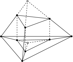
Figure 11: A vertical lift of the framework from Example 2.12.

Example 5.4.

The Maxwell-Cremona correspondence allows to prove the rigidity criterium for the framework from Example 2.12. The lines $a$, $b$, $c$ are concurrent if and only if the framework has a vertical lift, see Figure 11.

Remark 5.5.

The spaces of self-stresses, reciprocal diagrams, and polyhedral lifts have natural linear structures. The correspondences described in the proof of Theorem 5.3 are linear, see also [11].

Every graph $\Gamma$ has a geometric realization $|\Gamma|$: assign to the vertices points in $\mathbb{R}^{3}$ in general position, and to the edges the segments between those points. A map $\Gamma_{0}\to\mathbb{R}^{2}$ can be extended to a map $|\Gamma|\to\mathbb{R}^{2}$ by affine interpolation. We call this the rectilinear extension. If the rectilinear extension is an embedding, then every face of $\Gamma$ (viewed as a cycle of edges) becomes a polygon. In this case there is one face that is the union of all the other faces; we call it the exterior face (the term comes from the identification of $\mathbb{R}^{2}$ with a punctured sphere). The edges of the exterior face are called boundary edges, all of the other edges are called interior edges.

Theorem 5.6.

Let $(\Gamma,p)$ be a framework in $\mathbb{R}^{2}$ with a planar $3$-connected graph $\Gamma$ and such that the rectilinear extension of $p$ to $|\Gamma|$ provides an embedding of $\Gamma$ into $\mathbb{R}^{2}$ with convex faces. Then the following conditions are equivalent:

1. The framework has a self-stress that is positive on all interior edges and negative on all boundary edges.

2. The framework has a reciprocal diagram such that for every dual pair $(\alpha\beta,ij)$ the pair of vectors $(p_{j}-p_{i},m_{\beta}-m_{\alpha})$ is positively oriented if $ij$ is an interior edge and negatively oriented if $ij$ is a boundary edge.

3. The framework has a vertical polyhedral lift to a convex polytope.

4. The framework has a radial polyhedral lift to a convex polytope.

Proof.

It suffices to show that the constructions in the proof of Theorem 5.3 respect the above properties.

1) $\Leftrightarrow$ 2): Since a self-stress is related to a reciprocal diagram by the formula $m_{\beta}-m_{\alpha}=w_{ij}J(p_{j}-p_{i})$, the pair $(p_{j}-p_{i},m_{\beta}-m_{\alpha})$ is positively oriented if and only if $w_{ij}>0$.

2) $\Leftrightarrow$ 3): Since $m_{\beta}-m_{\alpha}=\operatorname{grad}(f_{\beta}-f_{\alpha})$, the pairs $(p_{j}-p_{i},m_{\beta}-m_{\alpha})$ for all interior edges $ij$ are positively oriented if and only if the piecewise linear function over the union of the interior faces defined by $f(x)=f_{\alpha}(x)$ for $x\in\alpha$ is convex. The graph of this function together with the lift of the exterior face (that covers the union of the interior faces) form a convex polytope.

3) $\Leftrightarrow$ 4): The projective image of a convex polytope (provided no point is sent to infinity) is a convex polytope. The orthogonal lift can be made disjoint from the plane that is sent to infinity by shifting in the vertical direction. ∎

Remark 5.7.

By adding a linear function to an orthogonal polyhedral lift we can achieve that the exterior face stays in $\mathbb{R}^{2}$. A convex polytope of this kind is called a convex cap. An example is given on Figure 11.

Remark 5.8.

The only self-intersections of the reciprocal diagram from Theorem 5.6 involve the edges $m_{\alpha_{0}}m_{\beta}$, where $\alpha_{0}$ is the exterior face of $\Gamma$ (and there is no way to get rid of all self-intersections unless $\Gamma$ is the graph of the tetrahedron). The reciprocal diagram can be represented without self-intersections by replacing every edge $m_{\alpha_{0}}m_{\beta}$ with a ray running from $m_{\beta}$ in the direction opposite to $m_{\alpha_{0}}$. Complexes of this sort are called spider webs in [53].

Non-crossing frameworks with non-crossing reciprocals (and thus with some non-convex faces) are studied in the article [40].

Remark 5.9.

The Dirichlet tesselation of a finite point set and the corresponding Voronoi diagram are a special case of a framework and a reciprocal diagram of the type described in Theorem 5.6. The vertical lift is given by $\tilde{p}_{i}=(p_{i},\|p_{i}\|^{2})$. The Voronoi diagram represents the reciprocal in the form of a spider web as described in the previous remark. A generalization of Dirichlet tesselations and Voronoi diagrams are weighted Delaunay tesselations and power diagrams. One of the definitions of a weighted Delaunay tesselation is a tesselation that possesses a vertical lift to a convex polytope. Thus one can a fifth equivalent condition to Theorem 5.6: the framework is a weighted Delaunay tesselation. For details see [3].

In [53] the spider webs were related to planar sections of spatial Delaunay tesselations.

Remark 5.10.

Not every convex tesselation and even not every triangulation of a convex polygon has a convex polyhedral lift, see [13, Chapter 7.1] for the “mother of all counterexamples”. Those that do are called coherent or regular triangulations (more generally, tesselations). There is a generalization to higher dimensions, see [13].

5.3 Maxwell-Cremona correspondence in spherical geometry

Definition 5.11.

Let $(\Gamma,p)$ be a framework in $\mathbb{S}^{2}$ with a planar $3$-connected graph $\Gamma$. A weak reciprocal diagram for $(\Gamma,p)$ is a framework $(\Gamma^{*},m)$ in $\mathbb{S}^{2}$ such that

1. for every dual pair $(\alpha\beta,ij)$ the geodesics $p_{i}p_{j}$ and $m_{\alpha}m_{\beta}$ are perpendicular;

2. for every incident pair $(\alpha,i)$ the distance between $m_{\alpha}$ and $p_{i}$ is different from $\frac{\pi}{2}$.

A strong reciprocal diagram is defined in the same way except that condition 2) is replaced by

1. for every incident pair $(\alpha,i)$ the distance between $m_{\alpha}$ and $p_{i}$ is less than $\frac{\pi}{2}$.

The reciprocity conditions can be rewritten as

$$\langle m_{\alpha},p_{i}\rangle\langle m_{\beta},p_{j}\rangle-\langle m_{\alpha},p_{j}\rangle\langle m_{\beta},p_{i}\rangle=0$$ (8)

$$\langle m_{\alpha},p_{i}\rangle\neq 0$$ (9)

$$\langle m_{\alpha},p_{i}\rangle>0$$ (9’)

The left hand side in (8) equals $\langle m_{\alpha}\times m_{\beta},p_{i}\times p_{j}\rangle$.

Definition 5.12.

Let $(\Gamma,p)$ be a framework in $\mathbb{S}^{2}$ with a planar $3$-connected graph $\Gamma$ and such that for every face $\alpha\in\Gamma_{2}$ the points $\{p_{i}\mid i\in\alpha\}$ are not collinear (that is, don’t lie on a great circle). A weak polyhedral lift of $(\Gamma,p)$ is a map $\tilde{p}\colon\Gamma_{0}\to\mathbb{R}^{3}$ such that

1. $\tilde{p}_{i}=a_{i}p_{i}$ for every $i\in\Gamma_{0}$, where $a_{i}\neq 0$;

2. for every face $\alpha\in\Gamma_{2}$ the points $\{\tilde{p}_{i}\mid i\in\alpha\}$ are coplanar;

3. the planes of the adjacent faces differ from each other.

A strong polyhedral lift is defined similarly but with $a_{i}>0$ in condition 1.

Theorem 5.13.

Let $(\Gamma,p)$ be a framework in $\mathbb{S}^{2}$ with a planar $3$-connected graph $\Gamma$ and such that for every face $\alpha\in\Gamma_{2}$ the points $\{p_{i}\mid i\in\alpha\}$ are not collinear. Then the following conditions are equivalent:

1. The framework has a self-stress that is non-zero on all edges.

2. The framework has a weak reciprocal diagram.

3. The framework has a weak polyhedral lift.

Proof.

1) $\Rightarrow$ 3): By Lemma 3.7, a self-stress $w$ gives rise to a map $\lambda\colon\Gamma_{1}\to\mathbb{R}$ such that

$$\sum_{j\in\Gamma_{0}}\lambda_{ij}p_{j}\parallel p_{i}\quad\text{for all }i\in\Gamma_{0}.$$ (10)

Pick an $\alpha_{0}\in\Gamma_{2}$ and define $\tilde{m}_{\alpha_{0}}\in\mathbb{R}^{3}$ arbitrarily. Define $\tilde{m}\colon\Gamma_{2}\to\mathbb{R}^{3}$ recursively: if $\tilde{m}_{\alpha}$ is already defined, then for every $\beta$ adjacent to $\alpha$ put

$$\tilde{m}_{\beta}=\tilde{m}_{\alpha}+\lambda_{ij}(p_{i}\times p_{j}),$$

where $(\alpha\beta,ij)$ is a consistently oriented dual pair. Equation (10) implies that the closing condition around every vertex $i$ holds:

$$\sum_{j}\lambda_{ij}(p_{i}\times p_{j})=0.$$

Thus we have a well-defined map $\tilde{m}\colon\Gamma_{2}\to\mathbb{R}^{3}$ with

$$\tilde{m}_{\beta}-\tilde{m}_{\alpha}\parallel p_{i}\times p_{j}$$

for any dual pair $(\alpha\beta,ij)$. In particular, $\tilde{m}_{\beta}-\tilde{m}_{\alpha}\perp p_{i}$, which implies that for every $i$ there is $c_{i}\in\mathbb{R}$ such that

$$\langle\tilde{m}_{\alpha},p_{i}\rangle=c_{i}$$

for all $\alpha$ incident to $i$. For a generic initial choice of $\tilde{m}_{\alpha_{0}}$ we have $c_{i}\neq 0$ for all $i$. If we put $\tilde{p}_{i}=\frac{p_{i}}{c_{i}}$, then we have

$$\langle\tilde{m}_{\alpha},\tilde{p}_{i}\rangle=1$$

for every incident pair $(\alpha,i)$. It follows that for every $\alpha\in\Gamma_{2}$ the points $\{\tilde{p}_{i}\mid i\in\alpha\}$ are coplanar and span a plane orthogonal to the vector $\tilde{m}_{\alpha}$. Due to $\lambda_{ij}\neq 0$ for every edge $ij$ the planes of adjacent faces are different, thus we have constructed a weak polyhedral lift of $(\Gamma,p)$.

3) $\Rightarrow$ 2): Let $M_{\alpha}\subset\mathbb{R}^{3}$ be the plane containing the points $\{\tilde{p}_{i}\mid i\in\alpha\}$. Since the points $\{p_{i}\mid i\in\alpha\}$ are not collinear, the plane $M_{\alpha}$ does not pass through the origin. Thus it has equation of the form

$$M_{\alpha}=\{x\in\mathbb{R}^{3}\mid\langle\tilde{m}_{\alpha},x\rangle=1\}$$

for some $\tilde{m}_{\alpha}\in\mathbb{R}^{3}$. In particular, for any dual pair $(\alpha\beta,ij)$ we have

$$\langle\tilde{m}_{\beta}-\tilde{m}_{\alpha},\tilde{p}_{i}\rangle=\langle\tilde{m}_{\beta}-\tilde{m}_{\alpha},\tilde{p}_{j}\rangle=0.$$

Hence the vector $\tilde{m}_{\beta}-\tilde{m}_{\alpha}$, and with it the plane spanned by $\tilde{m}_{\alpha}$ and $\tilde{m}_{\beta}$, is perpendicular to the plane spanned by $p_{i}$ and $p_{j}$. If we put $m_{\alpha}=\frac{\tilde{m}_{\alpha}}{\|\tilde{m}_{\alpha}\|}$, then the geodesic $m_{\alpha}m_{\beta}$ is perpendicular to the geodesic $p_{i}p_{j}$. Since $\langle\tilde{m}_{\alpha},\tilde{p}_{i}\rangle=1$, we have $\langle m_{\alpha},p_{i}\rangle\neq 0$. Thus $(\Gamma^{*},m)$ is a weak reciprocal diagram to $(\Gamma,p)$.

2) $\Rightarrow$ 3): Let $(\Gamma^{*},m)$ be a weak reciprocal diagram for $(\Gamma,p)$. We construct lifts $\tilde{m}$ and $\tilde{p}$ such that

$$\langle\tilde{m}_{\alpha},\tilde{p}_{i}\rangle=1$$ (11)

for every incident pair $(\alpha,i)$. The construction is recursive.

Pick $\alpha_{0}\in\Gamma_{2}$ and lift $m_{\alpha_{0}}$ arbitrarily. Due to (9), for every $i\in\alpha_{0}$ there is a lift $\tilde{p}_{i}$ of $p_{i}$ such that $\langle\tilde{m}_{\alpha_{0}},\tilde{p}_{i}\rangle=1$. If $\tilde{m}_{\alpha}$ is already defined, and $\beta$ is adjacent to $\alpha$, then let $ij$ be the edge dual to $\alpha\beta$. First determine the lift $\tilde{p}_{i}$ from the condition (11), and then determine the lift $\tilde{m}_{\beta}$ from the same condition with $\beta$ in place of $\alpha$. Note that if we use $p_{j}$ instead of $p_{i}$, then the result will be the same: due to the reciprocity conditions (8) and (9) we have

$$\langle\tilde{m}_{\alpha},\tilde{p}_{i}\rangle=\langle m_{\alpha},\tilde{p}_{j}\rangle\Rightarrow\langle\tilde{m}_{\beta},\tilde{p}_{i}\rangle=\langle\tilde{m}_{\beta},\tilde{p}_{j}\rangle.$$

This recursive procedure leads to well-defined lifts $\tilde{m}$ and $\tilde{p}$: going around a vertex $i$ does not change the value of $\tilde{m}_{\alpha}$ because both the initial and the final values satisfy (11).

3) $\Rightarrow$ 1): Let $\tilde{m}\colon\Gamma_{2}\to\mathbb{R}^{3}$ be the map constructed during the proof of the implication 3) $\Rightarrow$ 2). As it was shown, for every dual pair $(\alpha\beta,ij)$ the non-zero vector $\tilde{m}_{\beta}-\tilde{m}_{\alpha}$ is perpendicular to $p_{i}$ and $p_{j}$. Thus we have a map $\lambda\colon\Gamma_{1}\to\mathbb{R}$ such that

$$\tilde{m}_{\beta}-\tilde{m}_{\alpha}=\lambda_{ij}p_{i}\times p_{j}.$$

To determine the sign of $\lambda_{ij}$, we order the vertices so that the pair $(\alpha\beta,ij)$ is consistently oriented. Summing around a vertex $i$ of $\Gamma$ we obtain

$$p_{i}\times\sum_{j\in\Gamma_{0}}\lambda_{ij}p_{j}=0.$$

Hence $\sum_{j\in\Gamma_{0}}\lambda_{ij}p_{j}\parallel p_{i}$ and by Lemma 3.7 the map $\lambda$ gives rise to a non-zero self-stress on $(\Gamma,p)$. ∎

We don’t know what conditions on a framework and the stress guarantee the existence of a strong reciprocal diagram. At least it is necessary that the vertices of every face are contained in an open hemisphere. The next theorem shows that strong reciprocal diagrams correspond to strong polyhedral lifts.

Theorem 5.14.

Let $(\Gamma,p)$ be a framework in $\mathbb{S}^{2}$ as in Theorem 5.13. Then the following conditions are equivalent:

1. The framework has a strong reciprocal diagram.

2. The framework has a strong polyhedral lift.

Proof.

In the proof of 3) $\Rightarrow$ 2) in Theorem 5.13, note that for a strong lift $\tilde{p}$ the equation $\langle\tilde{m}_{\alpha},\tilde{p}_{i}\rangle=1$ implies $\langle m_{\alpha},p_{i}\rangle>0$, so that the reciprocal diagram constructed from a strong lift is strong itself.

In the proof of 2) $\Rightarrow$ 3) in Theorem 5.13, lift $m_{\alpha_{0}}$ strongly (that is scale it by a positive factor). Condition (11) implies that all $p_{i}$ with $i\in\alpha_{0}$ are also lifted strongly. The recursion propagates the strong lift to all $m_{\beta}$ and $p_{j}$. ∎

As in the Euclidean case (see the paragraph before Theorem 5.6), a spherical framework defines a geodesic extension, that is a map $|\Gamma|\to\mathbb{S}^{2}$ that sends every edge to an arc of a great circle. A geodesic extension is called a convex embedding of $\Gamma$ if it is an embedding and every face is a convex spherical polygon.

Theorem 5.15.

Let $(\Gamma,p)$ be a framework in $\mathbb{S}^{2}$ with a planar $3$-connected graph $\Gamma$ and such that its geodesic extension is a convex embedding. Then the following conditions are equivalent:

1. The framework has a self-stress that is positive on all edges.

2. The framework has a strong reciprocal diagram that embeds $\Gamma^{*}$ in $\mathbb{S}^{2}$ with convex faces.

3. The framework has a strong lift to a convex polyhedron.

Proof.

1) $\Rightarrow$ 3): In the proof of the corresponding implication in Theorem 5.13 we have $\lambda_{ij}>0$ for all edges $ij$. This implies that as we go around a vertex $i$, the vertices $\tilde{m}_{\alpha}$ for all $\alpha$ adjacent to $i$ form a convex polygon. The union of these polygons is the boundary of a convex polyhedron that contains $0$ in its interior. Its polar dual is a strong lift of $(\Gamma,p)$.

3) $\Rightarrow$ 2): A convex polyhedron that is a strong lift of $(\Gamma,p)$ contains $0$ in the interior. Thus its polar dual is also a convex polyhedron. The projection of the $1$-skeleton of the dual is a strong reciprocal diagram with convex faces.

2) $\Rightarrow$ 1): In a strong reciprocal diagram with convex faces the geodesics $m_{\alpha}m_{\beta}$ and $p_{i}p_{j}$ that correspond to a dual pair are consistently oriented. When we lift such a diagram as in the proof of 2) $\Rightarrow$ 3) $\Rightarrow$ 1) in Theorem 5.13, we obtain real numbers $\lambda_{ij}>0$ that provide a positive self-stress on $(\Gamma,p)$. ∎

The latter version of the spherical Maxwell-Cremona correspondence was described in [34].

Remark 5.16.

As in the Euclidean case, not every convex tesselation of the sphere has a convex polyhedral lift. The corresponding theory predates the theory of regular triangulations in the Euclidean space and was developed by Shephard [48] and McMullen [35]. See also [16].

5.4 Maxwell-Cremona correspondence in hyperbolic geometry

Let $(\Gamma,p)$ be a framework in $\mathbb{H}^{2}$ with a planar $3$-connected graph $\Gamma$. A reciprocal diagram is a framework $(\Gamma^{*},m)$ in $\mathbb{H}^{2}$ such that for every dual pair $(\alpha\beta,ij)$ the geodesics $m_{\alpha}m_{\beta}$ and $p_{i}p_{j}$ are perpendicular. In terms of the Minkowski scalar product this means

$$\langle m_{\alpha},p_{i}\rangle\langle m_{\beta},p_{j}\rangle-\langle m_{\alpha},p_{j}\rangle\langle m_{\beta},p_{i}\rangle=0.$$

Remark 5.17.

The above criterion of orthogonality of $m_{\alpha}m_{\beta}$ and $p_{i}p_{j}$ as well as its spherical analog (8) can be reformulated as follows. Diagonals in a spherical or hyperbolic quadrilateral with the side lengths $a,b,c,d$ in this cyclic order are orthogonal if and only if

$$\cos_{\mathbb{X}}a\cos_{\mathbb{X}}c=\cos_{\mathbb{X}}b\cos_{\mathbb{X}}d.$$

The diagonals of a Euclidean quadrilateral are orthogonal if and only if $a^{2}+c^{2}=b^{2}+d^{2}$.

Definition 5.18.

Let $(\Gamma,p)$ be a framework in $\mathbb{H}^{2}$ with a planar $3$-connected graph $\Gamma$ and such that for every face $\alpha\in\Gamma_{2}$ the points $\{p_{i}\mid i\in\alpha\}$ are not collinear. A polyhedral lift of $(\Gamma,p)$ is a map $\tilde{p}\colon\Gamma_{0}\to\mathbb{R}^{3}$ such that

1. $\tilde{p}_{i}=a_{i}p_{i}$ for every $i\in\Gamma_{0}$, where $a_{i}>0$;

2. for every face $\alpha\in\Gamma_{2}$ the points $\{\tilde{p}_{i}\mid i\in\alpha\}$ are contained in a space-like plane;

3. the planes of the adjacent faces differ from each other.

Theorem 5.19.

Let $(\Gamma,p)$ be a framework in $\mathbb{H}^{2}$ with a planar $3$-connected graph $\Gamma$ and such that for every face $\alpha\in\Gamma_{2}$ the points $\{p_{i}\mid i\in\alpha\}$ are not collinear. Then the following conditions are equivalent:

1. The framework has a self-stress that is non-zero on all edges.

2. The framework has a reciprocal diagram.

3. The framework has a polyhedral lift.

Proof.

1) $\Rightarrow$ 3): Proceed as in the proof of Theorem 5.13 to obtain a map $\tilde{m}\colon\Gamma_{2}\to\mathbb{R}^{3}$ such that

$$\tilde{m}_{\beta}-\tilde{m}_{\alpha}\parallel p_{i}\times p_{j}$$

(with the Minkowski cross-product) for every dual pair $(\alpha\beta,ij)$. By changing the position of $\tilde{m}_{\alpha_{0}}$ and scaling down the self-stress $w$ we can achieve that all $\tilde{m}_{\alpha}$ belong to the upper half of the light cone. Then the planes $\langle\tilde{m}_{\alpha},x\rangle=-1$ bound a polyhedron with space-like faces that is a polyhedral lift of $(\Gamma,p)$.

3) $\Rightarrow$ 2): Similarly to the proof of Theorem 5.13, let $\langle\tilde{m}_{\alpha},x\rangle=-1$ be an equation of the plane containing the points $\{\tilde{p}_{i}\mid i\in\alpha\}$. Since these planes are space-like, $\tilde{m}_{\alpha}$ are time-like, and since $\tilde{p}_{i}$ belongs to the upper half of the light cone, $\tilde{m}_{\alpha}$ also does. Hence $(\Gamma^{*},m)$ is a reciprocal diagram in $\mathbb{H}^{2}$.

2) $\Rightarrow$ 3): The proof is the same as in Theorem 5.13, we lift $(\Gamma,p)$ and $(\Gamma^{*},m)$ recursively and at the same time.

3) $\Rightarrow$ 1): Also the same as in Theorem 5.13, but with the Minkowski cross-product instead of the Euclidean. ∎

For a framework $(\Gamma,p)$ in $\mathbb{H}^{2}$ the geodesic extension $|\Gamma|\to\mathbb{H}^{2}$ is an analog of the rectilinear extension in the Euclidean case: an edge $ij$ of $\Gamma$ is mapped to the geodesic segment $p_{i}p_{j}$. If the geodesic extension is an embedding, then we define the interior and exterior faces and the interior and boundary edges as in the Euclidean case, see the paragraph before Theorem 5.6.

For a consistently oriented dual pair $(\alpha\beta,ij)$ we say that the lines $p_{i}p_{j}$ and $m_{\alpha}m_{\beta}$ are consistently oriented if the directed line $m_{\alpha}m_{\beta}$ is obtained from the directed line $p_{i}p_{j}$ through rotation by $\frac{\pi}{2}$ around their intersection point.

Theorem 5.20.

Let $(\Gamma,p)$ be a framework in $\mathbb{H}^{2}$ with a planar $3$-connected graph $\Gamma$ and such that the geodesic extension of $p$ to $|\Gamma|$ provides an embedding of $\Gamma$ into $\mathbb{H}^{2}$ with convex faces. Then the following conditions are equivalent:

1. The framework has a self-stress that is positive on all interior edges and negative on all boundary edges.

2. The framework has a reciprocal diagram such that for every consistently oriented dual pair $(\alpha\beta,ij)$ the lines $p_{i}p_{j}$ and $m_{\alpha}m_{\beta}$ are consistently oriented if $ij$ is an interior edge and non-consistently oriented if $ij$ is a boundary edge.

3. The framework has a polyhedral lift to a convex polytope in the Minkowski space.

Proof.

The proof consists in checking that the constructions in the proof of Theorem 5.19 respect the above properties. ∎

Remark 5.21.

A variant of the Maxwell-Cremona theorem for hyperbolic frameworks uses an orthogonal polyhedral lift to the co-Minkowski space instead of a radial polyhedral lift to the Minkowski space described above. For details on the co-Minkowski space see [17].

Remark 5.22.

If we allow the faces of the polyhedral lift to be time-like or light-like, then the vertices of the corresponding reciprocal diagram become de Sitter or ideal. Since the reciprocity is a symmetric notion, it is natural to allow de Sitter and ideal positions for the vertices of the framework as well. This puts us into the more general context of hyperbolic-de Sitter frameworks or point-line-horocycle frameworks, see Section 2.3.

References

- [1] A. D. Alexandrov. Convex polyhedra. Springer Monographs in Mathematics. Springer-Verlag, Berlin, 2005. Translated from the 1950 Russian edition by N. S. Dairbekov, S. S. Kutateladze and A. B. Sossinsky, With comments and bibliography by V. A. Zalgaller and appendices by L. A. Shor and Yu. A. Volkov.
- [2] L. Asimow and B. Roth. The rigidity of graphs. II. J. Math. Anal. Appl., 68(1):171–190, 1979.
- [3] F. Aurenhammer, R. Klein, and D.-T. Lee. Voronoi diagrams and Delaunay triangulations. World Scientific Publishing Co. Pte. Ltd., Hackensack, NJ, 2013.
- [4] W. Blaschke. Über affine Geometrie XXVI: Wackelige Achtflache. Math. Zeitschr., 6:85–93, 1920.
- [5] E. D. Bolker and B. Roth. When is a bipartite graph a rigid framework? Pacific J. Math., 90(1):27–44, 1980.
- [6] R. Bricard. Mémoire sur la théorie de l’octaèdre articulé. Journ. de Math. (5), 3:113–148, 1897.
- [7] A.-L. Cauchy. Sur les polygones et polyèdres, second mémoire. Journal de l’Ecole Polytechnique, 19:87–98, 1813.
- [8] R. Connelly. The rigidity of certain cabled frameworks and the second-order rigidity of arbitrarily triangulated convex surfaces. Adv. in Math., 37(3):272–299, 1980.
- [9] R. Connelly. Rigidity. In Handbook of convex geometry, Vol. A, pages 223–271. North-Holland, Amsterdam, 1993.
- [10] R. Connelly. Generic global rigidity. Discrete Comput. Geom., 33(4):549–563, 2005.
- [11] H. Crapo and W. Whiteley. Spaces of stresses, projections and parallel drawings for spherical polyhedra. Beiträge Algebra Geom., 35(2):259–281, 1994.
- [12] G. Darboux. Leçons sur la théorie générale des surfaces. III, IV. Les Grands Classiques Gauthier-Villars. Éditions Jacques Gabay, Sceaux, 1993.
- [13] J. A. De Loera, J. Rambau, and F. Santos. Triangulations, volume 25 of Algorithms and Computation in Mathematics. Springer-Verlag, Berlin, 2010. Structures for algorithms and applications.
- [14] M. Dehn. Über die Starrheit konvexer Polyeder. Math. Ann., 77:466–473, 1916.
- [15] Y. Eftekhari, B. Jackson, A. Nixon, B. Schulze, S.-i. Tanigawa, and W. Whiteley. Point-hyperplane frameworks, slider joints, and rigidity preserving transformations. https://arxiv.org/abs/1703.06844.
- [16] F. Fillastre and I. Izmestiev. Shapes of polyhedra, mixed volumes, and hyperbolic geometry. Mathematika, 63(1):124–183, 2017.
- [17] F. Fillastre and A. Seppi. Spherical, hyperbolic and other projective geometries: convexity, duality, transitions. https://arxiv.org/abs/1611.01065. 47 pages.
- [18] A. A. Gaifullin. Flexible cross-polytopes in spaces of constant curvature. Proc. Steklov Inst. Math., 286(1):77–113, 2014.
- [19] H. Gluck. Almost all simply connected closed surfaces are rigid. In Geometric topology (Proc. Conf., Park City, Utah, 1974), pages 225–239. Lecture Notes in Math., Vol. 438. Springer, Berlin, 1975.
- [20] I. Ivanova-Karatopraklieva, P. E. Markov, and I. K. Sabitov. Bending of surfaces. III. Fundam. Prikl. Mat., 12(1):3–56, 2006.
- [21] I. Ivanova-Karatopraklieva and I. K. Sabitov. Deformation of surfaces. I. In Problems in geometry, Vol. 23 (Russian), Itogi Nauki i Tekhniki, pages 131–184, 187. Akad. Nauk SSSR, Vsesoyuz. Inst. Nauchn. i Tekhn. Inform., Moscow, 1991. Translated in J. Math. Sci. 70 (1994), no. 2, 1685–1716.
- [22] I. Ivanova-Karatopraklieva and I. K. Sabitov. Bending of surfaces. II. J. Math. Sci., 74(3):997–1043, 1995. Geometry, 1.
- [23] I. Izmestiev. Spherical and hyperbolic conics. https://arxiv.org/abs/1702.06860. 50 pages.
- [24] I. Izmestiev. Projective background of the infinitesimal rigidity of frameworks. Geom. Dedicata, 140:183–203, 2009.
- [25] I. Izmestiev. Examples of infinitesimally flexible 3-dimensional hyperbolic cone-manifolds. J. Math. Soc. Japan, 63(2):581–598, 2011.
- [26] I. Izmestiev. Classification of flexible Kokotsakis polyhedra with quadrangular base. International Mathematics Research Notices, 2017(3):715–808, 2017.
- [27] B. Jackson and J. Owen. A characterisation of the generic rigidity of 2-dimensional point–line frameworks. Journal of Combinatorial Theory, Series B, 119:96 – 121, 2016.
- [28] B. Jessen. Orthogonal icosahedra. Nordisk Mat. Tidskr, 15:90–96, 1967.
- [29] A. Kokotsakis. Über bewegliche Polyeder. Math. Ann., 107(1):627–647, 1933.
- [30] G. Laman. On graphs and rigidity of plane skeletal structures. J. Engrg. Math., 4:331–340, 1970.
- [31] L. Lecornu. Sur l’equilibre des surfaces flexibles et inextensibles. J. de l’Éc. Pol. Cah. XLVIII. 1-109. (1880.) (1880)., 1880.
- [32] A.-M. Legendre. Éléments de géométrie, avec des notes, pages 321–334. Firmin Didot, 1794 (an II).
- [33] H. Liebmann. Ausnahmefachwerke und ihre Determinante. Münch. Ber., 50:197–227, 1920.
- [34] L. Lovász. Steinitz representations of polyhedra and the Colin de Verdière number. J. Combin. Theory Ser. B, 82(2):223–236, 2001.
- [35] P. McMullen. Representations of polytopes and polyhedral sets. Geometriae Dedicata, 2:83–99, 1973.
- [36] A. Möbius. Lehrbuch der Statik. Göschen, 1837.
- [37] A. F. Möbius. Kann von zwei dreiseitigen Pyramiden eine jede in Bezug auf die andere um- und eingeschrieben zugleich heißen? J. Reine Angew. Math., 3:273–278, 1828.
- [38] G. Nawratil. Flexible octahedra in the projective extension of the Euclidean 3-space. J. Geom. Graph., 14(2):147–169, 2010.
- [39] Y. Nishiyama. Miura folding: applying origami to space exploration. Int. J. Pure Appl. Math., 79(2):269–279, 2012.
- [40] D. Orden, G. Rote, F. Santos, B. Servatius, H. Servatius, and W. Whiteley. Non-crossing frameworks with non-crossing reciprocals. Discrete Comput. Geom., 32(4):567–600, 2004.
- [41] A. V. Pogorelov. Extrinsic geometry of convex surfaces. Translations of Mathematical Monographs. Vol. 35. Providence, R.I.: American Mathematical Society (AMS). VI, 1973.
- [42] L. Poinsot. Éléments de statique. Calixte-Volland, 1803 (an XII).
- [43] W. J. M. Rankine. On the application of barycentric perspective to the transformation of structures. Phil. Mag. Series, 4(26):387–388, 1863.
- [44] I. K. Sabitov. Local theory of bendings of surfaces [ MR1039820 (91c:53004)]. In Geometry, III, volume 48 of Encyclopaedia Math. Sci., pages 179–256. Springer, Berlin, 1992.
- [45] R. Sauer. Projektive Sätze in der Statik des starren Körpers. Math. Ann., 110(1):464–472, 1935.
- [46] R. Sauer and H. Graf. Über Flächenverbiegung in Analogie zur Verknickung offener Facettenflache. Math. Ann., 105(1):499–535, 1931.
- [47] E. Schönhardt. Über die Zerlegung von Dreieckspolyedern in Tetraeder. Math. Ann., 98:309–312, 1927.
- [48] G. C. Shephard. Spherical complexes and radial projections of polytopes. Israel J. Math., 9:257–262, 1971.
- [49] H. Stachel. Zur Einzigkeit der Bricardschen Oktaeder. J. Geom., 28(1):41–56, 1987.
- [50] E. Steinitz. Polyeder und Raumeinteilungen. In Encyclopädie der mathematischen Wissenschaften, Dritter Band: Geometrie, III.1.2., Heft 9, Kapitel 3 A B 12, pages 1–139. 1922.
- [51] W. Whiteley. Infinitesimal motions of a bipartite framework. Pacific J. Math., 110(1):233–255, 1984.
- [52] W. Whiteley. Infinitesimally rigid polyhedra. I. Statics of frameworks. Trans. Amer. Math. Soc., 285(2):431–465, 1984.
- [53] W. Whiteley, P. F. Ash, E. Bolker, and H. Crapo. Convex polyhedra, Dirichlet tessellations, and spider webs. In Shaping space, pages 231–251. Springer, New York, 2013.
- [54] H. Whitney. Congruent graphs and the connectivity of graphs. Amer. J. Math., 54(1):150–168, 1932.
- [55] G. M. Ziegler. Lectures on polytopes, volume 152 of Graduate Texts in Mathematics. Springer-Verlag, New York, 1995.