Solving post-Newtonian accurate Kepler Equation

Abstract

We provide an elegant way of solving analytically the third post-Newtonian (3PN) accurate Kepler equation, associated with the 3PN-accurate generalized quasi-Keplerian parametrization for compact binaries in eccentric orbits. An additional analytic solution is presented to check the correctness of our compact solution and we perform comparisons between our PN-accurate analytic solution and a very accurate numerical solution of the PN-accurate Kepler equation. We adapt our approach to compute crucial 3PN-accurate inputs that will be required to compute analytically both the time and frequency domain ready-to-use amplitude-corrected PN-accurate search templates for compact binaries in inspiralling eccentric orbits.

I Introduction

The emerging field of gravitational wave (GW) astronomy is expected to mature in the coming years and decades. This expectation is mainly due to the direct detection of GW signals, labeled GW150914 and GW151226 Abbott et al. (2016a, b), from the coalescence of two distinct binary black hole (BH) systems during the first observing run $(O1)$ of the advanced LIGO interferometer Abbott et al. (2016c). The astounding success of LISA pathfinder and maturing pulsar timing arrays ensure that multiwavelength GW astronomy will be achieved in the coming decades Armano et al. (2016); Burke-Spolaor (2015). Additionally, the coming years are expected to witness a substantial number of GW events due to the maturing of a network of ground-based GW observatories Abbott et al. (2016d, e). Coalescing BH binaries in quasicircular orbits should be the dominant GW sources for these observatories Abbott et al. (2016f, e, d). Preliminary investigations associated with the GW150914 event suggested that residual eccentricities $\leq 0.1$ at $10$ Hz would not introduce measurable deviations from the observed GW signal, modeled to be from a coalescing BH binary inspiralling along quasicircular orbits Abbott et al. (2016g). Indeed, a recent effort shows that BH binaries associated with the transient GW events GW150914 and GW151226 are likely to have orbital eccentricities below $0.15$ and $0.1$ at the GW frequency of $14$ Hz Huerta et al. (2017). However, there exist a number of astrophysically feasible scenarios in which binary BH systems can have moderate values of orbital eccentricities when their GWs enter observatories like aLIGO, as noted in Refs. Huerta et al. (2017); Tiwari et al. (2016).

There are ongoing efforts to model GWs associated with eccentric binary BH mergers Hinder et al. (2010); Bini and Damour (2012); Huerta et al. (2017). It is customary to employ the phasing prescription, developed in Refs. Damour et al. (2004); Königsdörffer and Gopakumar (2006), for describing the inspiral part of eccentric binary coalescence. This approach extends the early computations of Refs. Peters and Mathews (1963); Peters (1964) by incorporating in an efficient manner the effects of three timescales that are crucial to describe GWs from eccentric inspirals. The presence of three distinct timescales are essentially due to the use of the post-Newtonian (PN) approximation to describe the dynamics of these binaries. In the PN approximation, one invokes a certain gauge-invariant dimensionless parameter, namely $x\equiv{\left(\frac{Gm\omega}{c^{3}}\right)}^{2/3}$, where $m$ is the total binary mass while $\omega$ stands for the orbital (angular) frequency, as the expansion parameter. The use of $x$ is predominant while expressing the frequency and phase evolution of GWs from compact binaries as well as the amplitudes of their two polarization states $h_{+}$ and $h_{\times}$ Blanchet (2014). Let us recall that these three distinct timescales are associated with that of the orbital motion, periastron precession and radiation-reaction effects. In the GW phasing formalism of Refs. Damour et al. (2004); Königsdörffer and Gopakumar (2006), one models temporal variations in $h_{+}$ and $h_{\times}$ that occur at the orbital and periastron precession timescales in a semianalytical manner. This is possible due to the availability of a Keplerian-type parametric solution to the PN-accurate orbital dynamics of compact binaries. This solution provides a semianalytical description of the precessing eccentric orbits that are associated with the PN-accurate dynamics of compact binaries in noncircular orbits Memmesheimer et al. (2004).

The present paper provides an elegant analytical solution to the PN-accurate Kepler equation associated with the 3PN accurate generalized quasi-Keplerian parametrization, available in Ref. Memmesheimer et al. (2004). Specifically, we derive analytical 3PN-accurate infinite series expression for the eccentric anomaly $u$ in terms of the mean anomaly $l$. This solution requires us to derive compact PN-accurate infinite series expressions for certain trigonometric functions of the true anomaly $v$ in terms of $u$. We manipulate complex exponential representations of various trigonometric functions of $v$ and $u$ for these derivations. Another analytical solution to the 3PN-accurate Kepler equation is also provided to check the correctness of our solution. We invoke an improved version of Mikkola’s method, detailed in Refs. Mikkola (1987); Tessmer and Gopakumar (2007), to compare the accuracy of our analytical solution for various values of the orbital eccentricity. Our PN-accurate analytic solution shows excellent agreement with its numerical counterpart for moderate values of eccentricity.

We adapt the above computations to derive 3PN-accurate relations between various trigonometric functions of $v$ and $u$ in terms of $l$. These relations will be required to compute analytically the time-domain response function of GW observatories to eccentric inspirals. One requires PN-accurate amplitude-corrected $h_{\times}(t)$ and $h_{+}(t)$ expressions to obtain such ready-to-use response functions, namely $h(t)=F_{\times}\,h_{\times}(t)+F_{+}\,h_{+}(t)$, where $F_{\times}$ and $F_{+}$ are the so-called beam pattern functions of GW observatories. It is the practice of expressing $h_{\times}(t)$ and $h_{+}(t)$ as sums over various harmonics in $l$, as evident from Eqs. (3.3)-(3.10) in Ref. Yunes et al. (2009), that demands PN-accurate trigonometric functions of $v$ and $u$ in terms of the mean anomaly $l$. Note that the equations of Ref. Yunes et al. (2009) provide quadrupolar order GW polarization states associated with compact binaries moving along typical Keplerian (or Newtonian) eccentric orbits and require a solution to the classic Kepler equation and its subsidiary results. Our solution and the associated PN-accurate relations will be required to extend the results of Ref. Yunes et al. (2009) to 3PN order. We demonstrate the use of our PN-accurate relations by computing analytic 1PN-accurate amplitude-corrected expressions for $h_{+,\times}(l)$ that are accurate to leading order in orbital eccentricity.

Our prescription to compute analytic amplitude-corrected $h_{+,\times}(l)$ will also be required to obtain ready-to-use frequency domain GW response function for moderate eccentric inspirals. This ongoing effort is extending detailed computations, presented in Ref. Tanay et al. (2016), with the help of the postcircular expansion of PN-accurate eccentric orbits and the stationary phase approximation, detailed in Ref. Yunes et al. (2009).

In what follows, we sketch the derivation of a popular solution to the classic Kepler equation and provide its natural and elegant extension to tackle the 3PN-accurate Kepler equation. An equivalent but lengthy expression, influenced by Ref. Tessmer and Schäfer (2011), is presented in Appendix A while Appendix B provides the derivation of some of the crucial ingredients that are required for our analytic solution of the 3PN-accurate Kepler equation. We perform comparisons of our 3PN-accurate analytic solution to its numerical counterpart in a subsection of Sec. II. Section III presents our approach to obtain PN-accurate postcircular expansion of time-domain GW polarization states and we discuss its implications. Many detailed expressions, required for such an effort, and their brief derivations are provided in Appendices C, D and  E. Appendix F provides 1PN amplitude-corrected $h_{+,\times}$ expressions which extend the quadrupolar expressions of Ref. Wahlquist (1987).

II Derivation of analytic solution to PN-accurate Kepler Equation

We begin by sketching how F. W. Bessel invoked his now famous Bessel function to solve a demanding transcendental equation proposed by Johannes Kepler Colwell (1993). An elegant extension of Bessel’s approach to solve the 3PN-accurate Kepler equation is presented in Sec. II.2 and we probe its numerical accuracy in Sec. II.3.

II.1 The Bessel function approach to tackle the classic Kepler equation

We begin by reviewing the classical Keplerian parametrization that describes semianalytically the Newtonian-accurate orbital motion of a binary in noncircular orbits Colwell (1993); Damour and Deruelle (1985). In polar coordinates and in the center-of-mass reference frame, this approach provides a parametric description for an eccentric orbit of Newtonian dynamics using

$$r =a(1-e\cos u)\,,$$ (1a)

$$\phi-\phi_{0} =v\equiv 2\arctan\biggl{[}\biggl{(}\frac{1+e}{1-e}\biggr{)}^{1/2}\,\tan\frac{u}{2}\biggr{]}\,,$$ (1b)

where $r$ and $\phi$ define the components of the relative separation vector ${\bf r}=r(\cos\phi,\sin\phi,0)$. In the above equations, $a$ and $e$ stand for the semimajor axis and the eccentricity of the orbit, respectively. The auxiliary angles $u$ and $v$ are called eccentric and true anomaly. The classical Kepler equation defines the temporal evolution of these auxiliary angles and is given by

$$l\equiv n(t-t_{0})=u-e\,\sin u\,,$$ (2)

where $l$ is the mean anomaly and the mean motion $n$ is defined as $n=\frac{2\,\pi}{P}$, $P$ being the orbital period. The quantities $t_{0}$ and $\phi_{0}$ are some initial time and associated orbital phase. The conservative nature of the Newtonian orbital dynamics allows one to express the orbital elements $a$, $e$ and $n$ in terms of the Newtonian orbital energy and angular momentum. These expressions are given by

$$a =\frac{G\,m}{{(-2\,E)}}\,,$$ (3a)

$$e^{2} =1+2\,E\,h^{2}\,,$$ (3b)

$$n =\frac{{{(-2\,E)}}^{3/2}}{Gm}\,,$$ (3c)

where $E$ is the Newtonian orbital energy per unit reduced mass $\mu=m_{1}\,m_{2}/m$, $m_{1}$ and $m_{2}$ being the individual masses of the binary and $m=m_{1}+m_{2}$. The scaled angular momentum is given by $h=\frac{J}{G\,m}$, where $J$ is the reduced Newtonian orbital angular momentum.

Analytic solutions of the classical Kepler equation, namely $l=u-e\,\sin u$, had attracted the attention of several generations of distinguished mathematicians during the nineteenth and twentieth centuries Colwell (1993). In what follows, we sketch the derivation of the widely used solution involving the Bessel functions Watson (1922).

We start by expressing $u-l$ as a Fourier series in $l$:

$$u-l=e\,\sin u=\sum_{s=1}^{\infty}A_{s}\sin(sl)\,,$$ (4)

where the coefficients $A_{s}$ are given by

$$A_{s}=\frac{2}{\pi}\int_{0}^{\pi}(u-l)\sin(sl)dl\,.$$ (5)

Integrating by parts leads to

$$A_{s}= \frac{2}{\pi}\int_{0}^{\pi}(u(l)-l)\sin(sl)dl$$

$$= \frac{2}{s\pi}\int_{0}^{\pi}\cos(sl)du$$

$$= \frac{2}{s}\biggl{\{}\frac{1}{\pi}\,\int_{0}^{\pi}\cos(su-se\sin u)du\biggr{\}}\,.$$ (6)

The expression in the curly brackets can be identified with $J_{s}(se)$, namely the Bessel functions of the first kind. This allows us to write

$$u=l+\sum_{s=1}^{\infty}\frac{2}{s}J_{s}(se)\sin(sl)\,.$$ (7)

This expression provides the most popular solution of the transcendental Kepler equation. In what follows, we adapt a similar approach to tackle the PN-accurate Kepler equation.

II.2 3PN-accurate solution to PN-accurate Kepler equation

The post-Newtonian approach, heavily used to describe dynamics of astrophysical systems, incorporates general relativistic effects as perturbations to Newtonian dynamics. Einstein himself invoked the PN approach for describing the perihelion advance of Mercury Einstein (1916). We may treat the PN approximation as a computational tool for tackling the nonlinear Einsteinian prescription for gravity in terms of certain perturbative deviations from the linear Newtonian gravity. This approach involves an expansion in terms of a small parameter that is usually the squared ratio of the velocity of the matter distribution forming the gravitational field to the speed of light. For the inspiral dynamics of compact binaries this small parameter is equivalent to the above defined parameter $x$. At present, dynamics of compact binaries have been computed to the fourth PN order which provides general relativity based corrections to Newtonian description that are accurate to $x^{4}$ order (see Refs. Porto and Rothstein (2017); Damour and Jaranowski (2017); Foffa et al. (2017); Bernard et al. (2017); Damour et al. (2016) and references therein for the details of this herculean effort from various approaches).

Remarkably, it is possible to obtain a Keplerian-type parametric solution to the PN-accurate orbital dynamics of compact binaries in noncircular orbits Damour and Deruelle (1985); Damour and Schafer (1988); Schäfer and Wex (1993); Memmesheimer et al. (2004). At the third post-Newtonian order, the conservative orbital dynamics of compact binaries in eccentric orbits is specified by providing the following parametrization for the dynamical variables $r$ and $\phi$:

$$r =a_{r}\left(1-e_{r}\cos u\right)\,,$$ (8a)

$$\phi-\phi_{0} =(1+k)v+\left(f_{4\phi}+f_{6\phi}\right)\sin(2v)$$

$$\quad+\left(g_{4\phi}+g_{6\phi}\right)\sin(3v)+i_{6\phi}\sin(4v)$$

$$\quad+h_{6\phi}\sin(5v)\,,$$ (8b)

$$\text{where}\quad v =2\arctan\left[\left(\frac{1+e_{\phi}}{1-e_{\phi}}\right)^{1/2}\tan\frac{u}{2}\right]\,.$$ (8c)

A distinctive feature of the above two equations is the presence of different eccentricity parameters $e_{r}$ and $e_{\phi}$ for the radial and angular variables. These were introduced so that the PN-accurate parametrization looks “Keplerian” even at higher PN orders. The quantity $k$ provides the rate of periastron advance per orbital revolution. In the above equations, $a_{r}$, $e_{r}$, and $e_{\phi}$ are some 3PN accurate semimajor axis, radial eccentricity, and angular eccentricity, while $f_{4\phi}$, $f_{6\phi}$, $g_{4\phi}$, $g_{6\phi}$, $i_{6\phi}$, and $h_{6\phi}$ are some orbital functions of the energy and the angular momentum that enter at 2PN and 3PN orders. The explicit PN-accurate expressions of these quantities are available in Ref. Memmesheimer et al. (2004).

The following 3PN accurate Kepler equation links the eccentric anomaly $u$ to the mean anomaly $l=n\left(t-t_{0}\right)$

$$l= \;u-e_{t}\sin u+\left(g_{4t}+g_{6t}\right)(v-u)$$

$$+\left(f_{4t}+f_{6t}\right)\sin v+i_{6t}\sin(2v)+h_{6t}\sin(3v)\,.$$ (9)

This PN-accurate Kepler equation requires another eccentricity parameter, namely $e_{t}$, which is usually called the time eccentricity. Additionally, there are more orbital functions $g_{4t}$, $g_{6t}$, $f_{4t}$, $f_{6t}$, $i_{6t}$, and $h_{6t}$ that appear at 2PN and 3PN orders. The above-mentioned orbital elements and functions, expressible in terms of the conserved orbital energy, angular momentum, $m$ and $\eta$, are listed in Ref. Memmesheimer et al. (2004). We observe that the above parametric solution is usually referred to as the “generalized quasi-Keplerian” parametrization associated with the 3PN-accurate orbital dynamics. This is mainly due to the presence of these orbital functions that appear at 2PN and 3PN orders.

In what follows, we derive an elegant solution to the 3PN accurate Kepler equation, namely Eq. (II.2). It is possible to bring in a compact infinite series expansion, similar to Eq. (4), by invoking the following exact relations (see Appendix B for their derivations):

$$v-u= \;2\sum_{j=1}^{\infty}\frac{\beta_{\phi}^{j}}{j}\sin(ju)\,,$$ (10a)

$$\sin v= \;\frac{2\sqrt{1-e_{\phi}^{2}}}{e_{\phi}}\sum_{j=1}^{\infty}\beta_{\phi}^{j}\sin(ju)\,,$$ (10b)

$$\sin(2v)= \;\frac{4\sqrt{1-e_{\phi}^{2}}}{e_{\phi}^{2}}\sum_{j=1}^{\infty}\beta_{\phi}^{j}\left(j\sqrt{1-e_{\phi}^{2}}-1\right)\sin(ju)\,,$$ (10c)

$$\sin(3v)= \;\frac{2\sqrt{1-e_{\phi}^{2}}}{e_{\phi}^{3}}\sum_{j=1}^{\infty}\beta_{\phi}^{j}\Big{(}4-e_{\phi}^{2}$$

$$-6j\sqrt{1-e_{\phi}^{2}}+2j^{2}(1-e_{\phi}^{2})\Big{)}\sin(ju)\,,$$ (10d)

with $\beta_{\phi}=(1-\sqrt{1-e_{\phi}^{2}})/e_{\phi}$. These compact expressions allow us to express Eq. (II.2) as

$$l=u-e_{t}\sin u+\sum_{j=1}^{\infty}\alpha_{j}\sin(ju)\,,$$ (11)

where the explicit expressions for the PN-accurate orbital functions $\alpha_{j}$ can be extracted with the help of Eqs. (II.2) and (10). They are given by

$$\alpha_{j}= 2\beta_{\phi}^{j}\frac{\sqrt{1-e_{\phi}^{2}}}{e_{\phi}^{3}}\Bigg{(}(f_{4t}+f_{6t})e_{\phi}^{2}+\frac{(g_{4t}+g_{6t})e_{\phi}^{3}}{j\sqrt{1-e_{\phi}^{2}}}$$

$$+2i_{6t}e_{\phi}\left[j\sqrt{1-e_{\phi}^{2}}-1\right]$$

$$+h_{6t}\left[4-e_{\phi}^{2}-6j\sqrt{1-e_{\phi}^{2}}+2j^{2}(1-e_{\phi}^{2})\right]\Bigg{)}\,.$$ (12)

It is worth noting that the functional forms of $\alpha_{j}$ are identical in both the modified harmonic (MH) and Arnowitt-Deser-Misner (ADM) coordinates, since Eq. (II.2) takes an identical form in both gauges Memmesheimer et al. (2004). However, the explicit expressions for these orbital functions in terms of the conserved orbital energy and angular momentum or the parameters $x$ and $e_{t}$ differ.

The functional form of the PN-accurate Kepler equation, namely Eq. (11), allows us to write the following PN-accurate Fourier series for $u-l$

$$u-l=\sum_{s=1}^{\infty}A_{s}\sin(sl)\,,$$ (13)

where the coefficients $A_{s}$ are defined as

$$A_{s}=\frac{2}{\pi}\int_{0}^{\pi}(u-l)\sin(sl)dl\,.$$ (14)

Integrating by parts and using Eq. (11) gives

$$A_{s}= \;\frac{2}{\pi}\int_{0}^{\pi}(u-l)\sin(sl)dl$$

$$= \;\frac{2}{s\pi}\int_{0}^{\pi}\cos(sl)du$$

$$= \;\frac{2}{s\pi}\int_{0}^{\pi}\cos\Big{(}su-se_{t}\sin u+s\sum_{j=1}^{\infty}\alpha_{j}\sin(ju)\Big{)}du\,.$$ (15)

Note that the $\alpha_{j}$ contributions appear only at 2PN and 3PN orders as evident from Eq. (II.2). Therefore, we expand the sum in the cosine function of the above integral to the first order in $\alpha_{j}$. This leads to

$$A_{s}= \;\frac{2}{s\pi}\int_{0}^{\pi}\cos\left(su-se_{t}\sin u\right)du$$

$$-\frac{2}{\pi}\sum_{j=1}^{\infty}\alpha_{j}\int_{0}^{\pi}\sin\left(su-se_{t}\sin u\right)\sin(ju)du$$

$$= \;\frac{2}{s\pi}\int_{0}^{\pi}\cos\left(su-se_{t}\sin u\right)du$$

$$+\frac{1}{\pi}\sum_{j=1}^{\infty}\alpha_{j}\int_{0}^{\pi}\big{\{}\cos\left((s+j)u-se_{t}\sin u\right)$$

$$-\cos\left((s-j)u-se_{t}\sin u\right)\big{\}}du$$

$$= \;\frac{2}{s}J_{s}(se_{t})+\sum_{j=1}^{\infty}\alpha_{j}\left\{J_{s+j}(se_{t})-J_{s-j}(se_{t})\right\}\,,$$ (16)

where we employed the usual integral definitions for $J_{n}(x)$ to reach the last step. This step allows us to write down a simple and elegant solution to 3PN-accurate generalized Kepler equation in terms of Bessel functions as

$$u =l+\sum_{s=1}^{\infty}A_{s}\sin(sl)\,,$$ (17a)

$$A_{s} =\frac{2}{s}J_{s}(se_{t})+\sum_{j=1}^{\infty}\alpha_{j}\left\{J_{s+j}(se_{t})-J_{s-j}(se_{t})\right\}\,.$$ (17b)

Clearly, one requires explicit expressions for $\alpha_{j}$ in terms of $x$, $e_{t}$ and $\eta$ while employing our solution. The relevant expressions, valid for MH and ADM gauges, may be computed from Ref. Memmesheimer et al. (2004) as

$$\alpha_{j}^{\rm H}= \;\beta_{t}^{j}\Bigg{\{}x^{2}\Bigg{(}\frac{15-6\eta}{j\sqrt{1-e_{t}^{2}}}+\frac{15\eta-\eta^{2}}{4}\Bigg{)}+x^{3}\Bigg{(}\frac{2880\left(1+e_{t}^{2}\right)-\left(10880+2784e_{t}^{2}-123\pi^{2}\right)\eta+\left(960+1056e_{t}^{2}\right)\eta^{2}}{96j\left(1-e_{t}^{2}\right)^{3/2}}$$

$$+\frac{268800-\left(182192+1120e_{t}^{2}+4305\pi^{2}\right)\eta+\left(8260-11620e_{t}^{2}\right)\eta^{2}-1820\left(1-e_{t}^{2}\right)\eta^{3}}{3360\left(1-e_{t}^{2}\right)}$$

$$+j\frac{681\eta-199\eta^{2}+3\eta^{3}}{16\sqrt{1-e_{t}^{2}}}+j^{2}\frac{23\eta-73\eta^{2}+13\eta^{3}}{48}\Bigg{)}\Bigg{\}}\,,$$ (18a)

$$\alpha_{j}^{\rm A}= \;\beta_{t}^{j}\Bigg{\{}x^{2}\Bigg{(}\frac{15-6\eta}{j\sqrt{1-e_{t}^{2}}}-\frac{4\eta+\eta^{2}}{4}\Bigg{)}+x^{3}\Bigg{(}\frac{2880\left(1+e_{t}^{2}\right)-\left(10880+2784e_{t}^{2}-123\pi^{2}\right)\eta+\left(960+1056e_{t}^{2}\right)\eta^{2}}{96j\left(1-e_{t}^{2}\right)^{3/2}}$$

$$+\frac{7488-\left(7544-48e_{t}^{2}-3\pi^{2}\right)\eta+\left(1168+32e_{t}^{2}\right)\eta^{2}-52\left(1-e_{t}^{2}\right)\eta^{3}}{96\left(1-e_{t}^{2}\right)}$$

$$+j\frac{-18\eta+24\eta^{2}+3\eta^{3}}{16\sqrt{1-e_{t}^{2}}}+j^{2}\frac{13\eta^{3}}{48}\Bigg{)}\Bigg{\}}\,,$$ (18b)

where the superscripts ${\rm H}$ and ${\rm A}$ stand for the two gauges involved, namely the MH and ADM gauges. We note that $\beta_{t}=(1-\sqrt{1-e_{t}^{2}})/e_{t}$ is defined with the time eccentricity. To provide a check on our PN-accurate solution, we derive in Appendix A an alternate and less compact solution to the 3PN-accurate Kepler equation that is influenced by Ref. Tessmer and Schäfer (2011). We expand our two 3PN-accurate solutions to ${\cal O}(e_{t}^{40})$ to verify that they are identical at each order in $e_{t}$.

In what follows, we compare our solution with the 2PN-accurate $u(l)$ solution of Ref. Tessmer and Schäfer (2011). This solution in our notation reads

$$u= \;l+\sum_{s=1}^{\infty}A_{s}\sin(sl)\,,$$ (19a)

$$A_{s}= \;\frac{2}{s}J_{s}(se_{t})$$

$$-\sum_{j=1}^{\infty}\alpha_{j}\left\{J_{j-s}((j-s)e_{t})-J_{j+s}((j+s)e_{t})\right\}\,,$$ (19b)

with the constant coefficients $\alpha_{j}$ given by

$$\alpha_{j}= \;\frac{2\;g_{4t}}{j}\sum_{i=1}^{\infty}\beta_{\phi}^{i}\left\{J_{j-i}(je_{t})+J_{j+i}(je_{t})\right\}$$

$$+f_{4t}\sqrt{1-e_{t}^{2}}\left\{J_{j-1}(je_{t})-J_{j+1}(je_{t})\right\}\,.$$ (20)

We observe that two typos are persistent in Ref. Tessmer and Schäfer (2011) while trying to express $\sin v$ in terms of $l$. This is evident by comparing their Eq. (87) with our Eq. (C) or its equivalent that may be found in a classical treatise like Ref. Watson (1922). Additionally, the arguments of the Bessel functions should read $(k-n)e_{t}$ and $(k+n)e_{t}$ while going from steps 7 to 8 of Eq. (149) in Ref. Tessmer and Schäfer (2011). These corrections ensure that Eq. (19) is consistent with our elegant solution at 2PN order. To check the consistency of these two solutions, we expand Eqs. (17) and (19) around $e_{t}=0$. We have verified that they are in perfect agreement up to $\mathcal{O}(e_{t}^{40})$.

We observe that the approach of Ref. Tessmer and Schäfer (2011) results in a complicated PN-accurate expression for $u(l)$ as evident from our Eqs. (19) and (II.2). This is mainly due to the presence of infinite Bessel series in the constant $\alpha_{j}$. It turned out to be rather difficult to extend the prescription of Ref. Tessmer and Schäfer (2011) to 3PN order. This prompted us to develop a 3PN extension of Eq. (19) that requires PN-accurate compact relations, given by our Eqs. (10). This additional solution, detailed in Appendix A, provided an independent check for our 3PN-accurate elegant solution.

II.3 Comparison to numerical solution

In this subsection we compare our analytic solution against a very accurate way of solving the PN-accurate Kepler equation, detailed in Refs  Tessmer and Gopakumar (2007); Tanay et al. (2016). This numerical approach is based on an efficient and accurate (numerical) way of solving the classical Kepler equation, developed by Mikkola Mikkola (1987) and is valid for all $l$ and for $0\leq e_{t}\leq 1$. Mikkola’s method involves finding an analytic solution to certain cubic polynomial and a subsequent fourth-order iteration to improve on the initial guess for $u$. Its PN extension involves iteratively invoking the method to tackle PN-accurate Kepler equation, expressed in certain “quasiclassical” form (see Refs. Tessmer and Gopakumar (2007); Tanay et al. (2016) for details). We observe that the PN-accurate analytic solution is fully specified by providing values for $l$, $e_{t}$, $x$, and $\eta$. Our analytic solution is expected to be valid only up to certain values of the PN-expansion parameter $x$ and it will diverge for large values of $x$. Additionally, it will be useful to concentrate on the differences between $u$ and $l$ values due to the nature of Eq. (17). These considerations influenced us to probe how the fractional relative error, namely $|((u_{\textnormal{num}}-l)-(u_{\textnormal{anl}}-l))/(u_{\textnormal{num}}-l)|$, varies as a function of $e_{t}$ for few $x$ values while incorporating $200$ terms in the analytic solution. The results in MH gauge, displayed in Fig. 1, reveal that the relative error is small for moderate eccentricities and reasonable $x$ values. However, this error estimate can approach unity for $x$ values like $0.1$ even with moderate eccentricities ($e_{t}=0.7$). In any case, the maximum factional relative error is below $10\%$ for $e_{t}<0.5$ and $x=0.1$ for equal mass compact binaries.

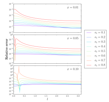
Figure 1: The fractional relative error $|((u_{\textnormal{num}}-l)-(u_{\textnormal{anl}}-l))/(u_{\textnormal{num}}-l)|$ as a function of the mean anomaly $l$ for different $e_{t}$ and $x$ values. We let $\eta=0.25$ and truncate the analytic series solution at $j=200$. $x\approx 0.01$ corresponds to a binary neutron star system entering the aLIGO band at 10 Hz, while a binary black hole system with masses around $10M_{\odot}$ enters at $x\approx 0.03$.

We invoke the more familiar integrated error over one period using the $L^{2}$ norm, namely

$$\lVert f\rVert_{L^{2}} =\left(\frac{1}{2\pi}\int_{0}^{2\pi}f^{2}dl\right)^{1/2}\,,$$ (21)

where $f$ stands for the above-mentioned fractional relative error. In Fig. 2, we show this error estimate as a function of $e_{t}$ for a number of $x$ values. We find that our $L^{2}$ norm error estimate is small ($<1\%$) for eccentricities up to $e_{t}=0.95$ for $x$ values relevant for the early inspiral phase like $x\approx 0.01$. However, it diverges quickly for higher $x$ values and this is true even for moderate $e_{t}$ values like $0.5$. A possible explanation is that this behavior happens when $e_{\phi}\sim e_{t}(1+x(4-\eta))+\mathcal{O}(x^{2})$ approaches unity. It is easy to infer that this happens when $e_{t}\approx 1/(1+4x)$ and this is consistent with our plots.

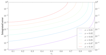
Figure 2: Integrated relative error as a function of $e_{t}$ for different $x$ values. The other parameters are as in Fig. 1.

In what follows, we introduce a new parameter to specify cleanly where our analytic solution is accurate, trustable and devoid of the above divergences. This post-Newtonian parameter is defined to be

$$y=\frac{(Gm\omega)^{1/3}}{\sqrt{1-e_{t}^{2}}}\,.$$ (22)

It smoothly goes to the standard post-Newtonian parameter $x^{1/2}$ in the circular limit.

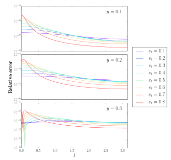
Figure 3: Relative error $|((u_{\textnormal{num}}-l)-(u_{\textnormal{anl}}-l))/(u_{\textnormal{num}}-l)|$ as a function of the mean anomaly $l$ for different $e_{t}$ and $y$ values. In the circular limit $y=0.1$ corresponds to $x=0.01$ and $y=0.316$ to $x=0.1$.

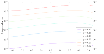
Figure 4: Integrated relative error as a function of the eccentricity $e_{t}$ for different $y$.

We plot in Fig. 3 the fractional relative error as a function of $l$ for several $e_{t}$ and few $y$ values. The sharp maxima, visible in Fig. 1, are absent in such $y$ plots and the maximum relative error is less than $1\%$ for large $y$ values like $0.3$. This is repeated in Fig. 4 for the integrated error as function of $e_{t}$ for several $y$ values. We again find smooth behavior and noticeably lower error estimates (less than $1\%$) for high $y$ and $e_{t}$ values.

In Figs. 1 to 4 we only considered equal mass binaries. We found similar behavior for Neutron star-black hole binaries ($\eta\sim 0.1$). These estimates suggest that our analytic solution should be accurate to compute analytic PN-accurate $h_{+,\times}(l)$ expressions for moderately eccentric inspirals. This is what we pursue in the next section.

III Inputs to compute analytic time-domain amplitude-corrected $h_{+,\times}(l)$

In this section we derive inputs that will be required to compute 3PN-accurate amplitude-corrected expressions for the time-domain $h_{+,\times}$ as a sum over harmonics in $l$. These PN-accurate results, as expected, will also be required to obtain amplitude corrected Fourier-domain inspiral templates with the help of Refs. Yunes et al. (2009); Tanay et al. (2016). Such PN-accurate input expressions can be regarded as nontrivial corollaries to our analytical solution to the 3PN-accurate Kepler equation. The various Fourier series coefficients derived in this section are given in a Mathematica Notebook in the Supplemental Material sup .

We begin by listing quadrupolar, Newtonian order expressions for $h_{+,\times}$ associated with nonspinning compact binaries in eccentric orbits, adapted from Gopakumar and Iyer (2002); Damour et al. (2004),

$$h_{+}^{0}= \,\frac{G\,m\,\eta}{2\,R^{\prime}\,c^{2}}\frac{x}{(1-e_{t}\cos u)^{2}}\Big{\{}s_{i}^{2}\left(-e_{t}^{2}+2e_{t}\cos u-e_{t}^{2}\cos(2u)\right)$$

$$-\left(1+c_{i}^{2}\right)\Big{\{}\left[4-3e_{t}^{2}-2e_{t}\cos u+e_{t}^{2}\cos(2u)\right]\cos(2\Phi)-4\sin u\,e_{t}\left(1-e_{t}^{2}\right)^{1/2}\sin(2\Phi)\Big{\}}\Big{\}}\,,$$ (23a)

$$h_{\times}^{0}= \,\frac{G\,m\,\eta}{R^{\prime}\,c^{2}}\frac{x\,c_{i}}{(1-e_{t}\cos u)^{2}}\left\{\left[4-3e_{t}^{2}-2e_{t}\cos u+e_{t}^{2}\cos(2u)\right]\sin(2\Phi)+4\sin u\,e_{t}\left(1-e_{t}^{2}\right)^{1/2}\cos(2\Phi)\right\}\,,$$ (23b)

where $R^{\prime}$ is the luminosity distance and $\Phi=\beta-\phi$. The source direction is specified by $(\iota,\beta)$ while $c_{i}=\cos\iota$, $s_{i}=\sin\iota$. We introduce $\Phi$ that combines the orbital phase $\phi$ with $\beta$. The orbital phase is specified by employing 3PN-accurate generalized quasi-Keplerian parametrization and it reads

$$\phi-\phi_{0}= \;(1+k)v+(f_{4\phi}+f_{6\phi})\sin(2v)$$

$$+(g_{4\phi}+g_{6\phi})\sin(3v)+i_{6\phi}\sin(4v)+h_{6\phi}\sin(5v)\,.$$ (24)

It is customary to split $\phi$ into an angle $\lambda$, which is linear in $l$, and $W(l)$, which is $2\pi$ periodic in $l$ Gopakumar and Iyer (2002); Damour et al. (2004). This allows us to write

$$\phi= \;\lambda+W(l)\,,$$ (25a)

$$\lambda= \;\phi_{0}+(1+k)l\,,$$ (25b)

$$W(l)= \;(1+k)(v-l)+(f_{4\phi}+f_{6\phi})\sin(2v)$$

$$+(g_{4\phi}+g_{6\phi})\sin(3v)+i_{6\phi}\sin(4v)+h_{6\phi}\sin(5v)\,.$$ (25c)

This split of $\phi$ is done to incorporate the advance of periastron explicitly into the GW phase evolution and its implications are discussed in Refs. Gopakumar and Iyer (2002); Tessmer and Gopakumar (2007). A close inspection of Eqs. (23) reveals that we need to express the cosine and sine of $W(l)$ and $(1-e_{t}\cos u)^{-2}$ as functions of the mean anomaly $l$ to obtain $h_{+,\times}$ as a sum over harmonics in $l$. It is not very difficult to infer that the derivations of such series expressions demand additional PN-accurate Fourier series of $\sin(ju)$, $\cos(ju)$, $\sin(jv)$ and $\cos(jv)$. In what follows, we tackle these challenges.

III.1 PN-accurate Fourier series expressions for various trigonometric functions of $u$,$v$ and $W$

We begin by deriving explicit expressions for the coefficients $\sigma_{s}^{ju}$ and $\zeta_{s}^{ju}$ such that 3PN-accurate Fourier series for $\sin(ju)$ and $\cos(ju)$ can be expressed as

$$\sin(ju) =\sum_{s=1}^{\infty}\sigma_{s}^{ju}\sin(sl)\,,$$ (26a)

$$\cos(ju) =\sum_{s=0}^{\infty}\zeta_{s}^{ju}\cos(sl)\,.$$ (26b)

We adopt certain $3$ indices notation to keep track of a number of coefficients that will be derived in this subsection. Let us emphasize that both $\sigma_{s}^{ju}$ and $\zeta_{s}^{ju}$ are not functions of $u$. We briefly describe how these Fourier coefficients are calculated in the Keplerian parametrization. The Fourier coefficients $\sigma_{s}^{ju}$ are defined as

$$\sigma_{s}^{ju}= \;\frac{2}{\pi}\int_{0}^{\pi}\sin(ju)\sin(sl)dl$$

$$= \;\frac{2j}{\pi s}\int_{0}^{\pi}\cos(ju)\cos(sl)du$$

$$= \;\frac{j}{\pi s}\int_{0}^{\pi}\big{\{}\cos((s-j)u-se\sin u)$$

$$+\cos((s-j)u-se\sin u)\big{\}}du$$

$$= \;\frac{j}{s}\left\{J_{s+j}(se)+J_{s-j}(se)\right\}\,,$$ (27)

where we employed the Newtonian Kepler equation $l=u-e\sin u$ and invoked the standard integral definition of Bessel functions of the first kind.

To extend it to 3PN order, we write our PN-accurate Kepler equation as $l=u-e_{t}\,\sin u+\sum_{j}\alpha_{j}\sin(ju)$, due to Eq. (11). We adapt the calculation to obtain $A_{s}$, detailed in Sec. II.2, by expanding $\cos((s+j)u-se_{t}\sin u+s\sum_{j}\alpha_{j}\sin(ju))$ in terms of the small parameters $\alpha_{j}$. The resulting 3PN-accurate Fourier series for $\sin(ju)$ reads

$$\sin(ju)= \;\sum_{s=1}^{\infty}\sigma_{s}^{ju}\sin(sl)\,,$$ (28a)

$$\sigma_{s}^{ju}= \;\frac{j}{s}\left\{J_{s+j}(se_{t})+J_{s-j}(se_{t})\right\}$$

$$+\frac{j}{2}\sum_{i=1}^{\infty}\alpha_{i}\big{\{}J_{s+j+i}(se_{t})-J_{s+j-i}(se_{t})$$

$$+J_{s-j+i}(se_{t})-J_{s-j-i}(se_{t})\big{\}}\,.$$ (28b)

Following similar steps, we can easily obtain 3PN-accurate Fourier series for $\cos(ju)$ as

$$\cos(ju)= \;\sum_{s=0}^{\infty}\zeta_{s}^{ju}\cos(sl)\,,$$ (29a)

$$\zeta_{0}^{ju}= \;\frac{1}{2}\left(-e_{t}\,\delta_{j1}+\alpha_{j}j\right)\,,$$ (29b)

$$\zeta_{s}^{ju}= \;\frac{j}{s}\left\{J_{s-j}(se_{t})-J_{s+j}(se_{t})\right\}$$

$$+\frac{j}{2}\sum_{i=1}^{\infty}\alpha_{i}\big{\{}J_{s-j+i}(se_{t})-J_{s-j-i}(se_{t})$$

$$-J_{s+j+i}(se_{t})+J_{s+j-i}(se_{t})\big{\}}\,,$$ (29c)

where $\delta_{j1}$ stands for the standard Kronecker delta. It is possible to provide a compact expression for $e^{iju}$ by combining the above results for $\cos(ju)$ and $\sin(ju)$ as $e^{iju}=\cos(ju)+i\sin(ju)$. The resulting expression is given by

$$e^{iju}= \;\sum_{s=-\infty}^{\infty}\epsilon_{s}^{ju}\,e^{isl}\,,$$ (30a)

$$\epsilon_{0}^{ju}= \;\frac{1}{2}\left(-e_{t}\,\delta_{j1}+\alpha_{j}j\right)\,,$$ (30b)

$$\epsilon_{s}^{ju}= \;\frac{j}{s}J_{s-j}(se_{t})$$

$$+\frac{j}{2}\sum_{k=1}^{\infty}\alpha_{k}\left\{J_{s-j+k}(se_{t})-J_{s-j-k}(se_{t})\right\}\,.$$ (30c)

We now move to derive the Fourier series of $\sin(jv)$ and $\cos(jv)$ in terms of the mean anomaly $l$ with the help of the above expressions. The plan is to write down a series expansion for $\sin(jv)$ in terms of $u$ as

$$\sin(jv) =\sum_{s=1}^{\infty}\mathcal{E}_{s}^{j}\sin(su)\,.$$ (31)

The above form is justified by our computations as detailed in Appendix B. We invoke the Fourier series of $\sin(ju)$, given by Eq. (28a), to obtain

$$\sin(jv) =\sum_{s=1}^{\infty}\sigma_{s}^{jv}\sin(sl)\,,$$ (32a)

$$\sigma_{s}^{jv} =\sum_{k=1}^{\infty}\mathcal{E}_{k}^{j}\sigma_{s}^{ku}\,,$$ (32b)

where $\mathcal{E}_{k}^{j}$ is given by Eqs. (74). Following similar arguments, we obtain PN-accurate results for $\cos(jv)$ as

$$\cos(jv) =\sum_{s=0}^{\infty}\zeta_{s}^{jv}\cos(sl)\,,$$ (33a)

$$\zeta_{s}^{jv} =\sum_{k=0}^{\infty}\mathcal{E}_{k}^{j}\zeta_{s}^{ku}\,,$$ (33b)

and $e^{ijv}$ as

$$e^{ijv} =\sum_{s=-\infty}^{\infty}\epsilon_{s}^{jv}e^{isl}\,,$$ (34a)

$$\epsilon_{s}^{jv} =\sum_{k=0}^{\infty}\mathcal{E}_{k}^{j}\epsilon_{s}^{ku}\,.$$ (34b)

We are now in a position to derive 3PN-accurate Fourier series expressions for $\cos(mW)$ and $\sin(mW)$. The starting point of our derivation is the following equation

$$W(l)= \;\sum_{s=1}^{\infty}\mathcal{W}_{s}\sin(sl)\,,$$ (35a)

$$\mathcal{W}_{s}= \;(1+k)B_{s}+(f_{4\phi}+f_{6\phi})\sigma_{s}^{2v}$$

$$+(g_{4\phi}+g_{6\phi})\sigma_{s}^{3v}+i_{6\phi}\sigma_{s}^{4v}+h_{6\phi}\sigma_{s}^{5v}\,.$$ (35b)

This equation arises from the 3PN-accurate expression for $W(l)$ given in Ref. Damour et al. (2004)

$$W(l)= \;(1+k)(v-l)+(f_{4\phi}+f_{6\phi})\sin(2v)$$

$$+(g_{4\phi}+g_{6\phi})\sin(3v)+i_{6\phi}\sin(4v)+h_{6\phi}\sin(5v)\,,$$ (36)

and our earlier derived series expressions for $\sin(jv)$, as well as a series expression for the true anomaly $v-l$, derived in Appendix C. We list these relevant expressions again

$$v-l =\sum_{s=1}^{\infty}B_{s}\sin(sl)\,,$$ (37a)

$$\sin(jv) =\sum_{s=1}^{\infty}\sigma_{s}^{jv}\sin(sl)\,.$$ (37b)

A straightforward computation that employs the above three infinite series expressions leads to the following Fourier series of $e^{imW}$ in terms of $l$:

$$e^{imW} =\sum_{n=-\infty}^{\infty}\mathcal{P}_{n}^{mW}e^{inl}\,.$$ (38)

The Fourier coefficients $\mathcal{P}_{n}^{mW}$ are given in Appendix E, where we describe the derivation of Eq. (38) in detail. It is then fairly routine to extract Fourier series of $\cos(mW)$ as

$$\cos(mW) =\sum_{n=0}^{\infty}\mathcal{C}_{n}^{mW}\cos(nl)\,,$$ (39a)

$$\mathcal{C}_{0}^{mW} =\mathcal{P}_{0}^{mW}\,,$$ (39b)

$$\mathcal{C}_{n}^{mW} =\mathcal{P}_{n}^{mW}+\mathcal{P}_{-n}^{mW}\,,$$ (39c)

and $\sin(mW)$ is given by

$$\sin(mW) =\sum_{n=1}^{\infty}\mathcal{S}_{n}^{mW}\sin(nl)\,,$$ (40a)

$$\mathcal{S}_{n}^{mW} =\mathcal{P}_{n}^{mW}-\mathcal{P}_{-n}^{mW}\,.$$ (40b)

Finally, we turn our attention to the derivation of $(1-e_{t}\cos u)^{-n}$. We adapt and extend the approach of Ref. Tessmer and Schäfer (2011) to obtain 3PN-accurate Fourier series of $(1-e_{t}\cos u)^{-n}$. Adapting the relevant result in Ref. Tessmer and Schäfer (2011), we write

$$\frac{1}{(1-e_{t}\cos u)^{n}}= \;\sum_{j=0}^{\infty}b^{n}_{j}\cos(ju)\,,$$ (41a)

$$b^{n}_{0}= \;{}_{2}F_{1}\left(\frac{n}{2},\frac{n+1}{2};1;e_{t}^{2}\right)\,,$$ (41b)

$$b^{n}_{j}= \;\frac{e_{t}^{j}}{2^{j-1}}\binom{n+j-1}{j}$$

$$\times{}_{2}F_{1}\left(\frac{n+j}{2},\frac{n+j+1}{2};j+1;e_{t}^{2}\right)\,,$$ (41c)

where ${}_{2}F_{1}$ stands for the ordinary hypergeometric function. Combining the above expression with the results for $\cos(ju)$, we get a 3PN-accurate Fourier series for $1/(1-e_{t}\cos u)^{n}$ as

$$\frac{1}{(1-e_{t}\cos u)^{n}}= \;\sum_{j=0}^{\infty}\mathcal{A}_{j}^{n}\cos(jl)\,,$$ (42a)

$$\mathcal{A}_{j}^{n}= \;\sum_{k=0}^{\infty}b_{k}^{n}\zeta_{j}^{ku}\,.$$ (42b)

In the next subsection, we apply the 1PN version of these results to demonstrate their utility in computing analytic $h_{+,\times}$ as a sum over harmonics in $l$.

III.2 Analytic $h_{+,\times}(l)$ via small eccentricity expansion

The plan is to apply the above derived PN-accurate series expansions to compute analytic 1PN-accurate amplitude-corrected expressions for $h_{+,\times}(l)$ in the small $e_{t}$ approximation. We begin from the exact 1PN-accurate amplitude-corrected $h_{+,\times}$ expressions that we symbolically write as

$$h_{+,\times} =\frac{G\,m\,\eta}{R^{\prime}\,c^{2}}x\left\{H^{0}_{+,\times}+x^{0.5}\,H^{0.5}_{+,\times}+x\,H^{1}_{+,\times}\right\}\,.$$ (43)

$H^{i}_{+,\times}$ are functions of $\Phi=\beta-\phi=\beta-(\lambda+W)$ and $u$. At the Newtonian order, explicit $H^{0}_{+,\times}$ expressions can be extracted from Eqs. (23), and we list the higher order terms that appear at $0.5$PN and 1PN orders in Appendix F. With the help of 1PN versions of the various relations derived in the previous subsection, we obtain

$$h_{+,\times}= \;\frac{G\,m\,\eta}{R^{\prime}\,c^{2}}x\sum_{p,q=0}^{\infty}\Big{\{}\left[a_{+,\times}^{p,q}\cos(pl)+b_{+,\times}^{p,q}\sin(pl)\right]\cos(q\lambda)$$

$$+\left[c_{+,\times}^{p,q}\cos(pl)+d_{+,\times}^{p,q}\sin(pl)\right]\sin(q\lambda)\Big{\}}\,.$$ (44)

To show a glimpse of our final result, we display certain 1PN-accurate Fourier coefficients, truncated at ${\cal O}(e_{t}^{3})$:

$$a^{0,1}_{+}= \;c_{1\beta}\,s_{i}\,\delta\,\sqrt{x}\left[-\frac{1}{4}\left(1+c_{i}^{2}\right)\left(1+2e_{t}^{2}\right)-1+2e_{t}^{2}\right]\,,$$ (45a)

$$a^{0,2}_{+}= \;c_{2\beta}\bigg{\{}\left(1+c_{i}^{2}\right)\left(-2+5e_{t}^{2}\right)+x\bigg{[}\frac{8}{3}\left(1-5e_{t}^{2}\right)\left(1-3\eta\right)$$

$$+\left(1+c_{i}^{2}\right)\left(3+\frac{11\eta}{3}+\frac{1}{6}e_{t}^{2}\left(315-151\eta\right)+\frac{2}{3}s_{i}^{2}\left(1+e_{t}^{2}\right)\left(1-3\eta\right)\right)\bigg{]}\bigg{\}}\,,$$ (45b)

$$a^{0,3}_{+}= \;\frac{9}{4}\,c_{3\beta}\,s_{i}\,\left(1+c_{i}^{2}\right)\delta\,\sqrt{x}\left(1-6e_{t}^{2}\right)\,,$$ (45c)

$$a^{0,4}_{+}= \;-\frac{8}{3}\,c_{4\beta}\,s_{i}^{2}\,\left(1+c_{i}^{2}\right)x\left(1-3\eta\right)\left(1-11e_{t}^{2}\right)\,,$$ (45d)

$$c^{0,1}_{+}= \;s_{1\beta}\,s_{i}\,\delta\,\sqrt{x}\left[-\frac{1}{4}\left(1+c_{i}^{2}\right)\left(1+2e_{t}^{2}\right)-1+2e_{t}^{2}\right]\,,$$ (45e)

$$c^{0,2}_{+}= \;s_{2\beta}\bigg{\{}\left(1+c_{i}^{2}\right)\left(-2+5e_{t}^{2}\right)+x\bigg{[}\frac{8}{3}\left(1-5e_{t}^{2}\right)\left(1-3\eta\right)$$

$$+\left(1+c_{i}^{2}\right)\left(3+\frac{11\eta}{3}+\frac{1}{6}e_{t}^{2}\left(315-151\eta\right)+\frac{2}{3}s_{i}^{2}\left(1+e_{t}^{2}\right)\left(1-3\eta\right)\right)\bigg{]}\bigg{\}}\,,$$ (45f)

$$c^{0,3}_{+}= \;\frac{9}{4}\,s_{3\beta}\,s_{i}\,\left(1+c_{i}^{2}\right)\delta\,\sqrt{x}\left(1-6e_{t}^{2}\right)\,,$$ (45g)

$$c^{0,4}_{+}= \;-\frac{8}{3}\,s_{4\beta}\,s_{i}^{2}\,\left(1+c_{i}^{2}\right)x\left(1-3\eta\right)\left(1-11e_{t}^{2}\right)\,,$$ (45h)

where $c_{k\beta}$ and $s_{k\beta}$ stand for $\cos(k\beta)$ and $\sin(k\beta)$ and we list only those coefficients that survive in the circular limit. We have verified that these coefficients are consistent with the 1PN-accurate amplitude-corrected $h_{+,\times}$ for quasicircular inspirals, provided in Ref. Blanchet et al. (1996). This exercise demonstrates the ability of our inputs to compute analytic PN-accurate amplitude-corrected expressions for $h_{+,\times}$ as a sum over harmonics in $l$.

Another important check of our approach is that we should also be able to reproduce Eqs. (3.6)-(3.10) in Ref. Yunes et al. (2009) while restricting our attention to the quadrupolar order $h_{+,\times}$ from eccentric binaries in Newtonian eccentric orbits. We use our Eq. (23) which provides the quadrupolar order $h_{+,\times}$ and the Newtonian version of our results from the previous subsection to obtain

$$h^{0}_{+,\times} =-\frac{G\,m\,\eta}{c^{2}\,R^{\prime}}x\sum_{p=0}^{\infty}\left[\mathcal{C}_{+,\times}^{p}\cos(pl)+\mathcal{S}_{+,\times}^{p}\sin(pl)\right]\,.$$ (46)

We list below $p=1$ coefficients accurate to ${\cal O}(e^{8})$:

$$\mathcal{C}_{+}^{1}= \;s_{i}^{2}\left(-e+\frac{e^{3}}{8}-\frac{e^{5}}{192}+\frac{e^{7}}{9216}\right)+c_{2\beta}(1+c_{i}^{2})$$

$$\times\left(-\frac{3e}{2}+\frac{2e^{3}}{3}-\frac{37e^{5}}{768}+\frac{11e^{7}}{7680}\right)\,,$$ (47a)

$$\mathcal{S}_{+}^{1}= \;s_{2\beta}(1+c_{i}^{2})$$

$$\times\left(-\frac{3e}{2}+\frac{23e^{3}}{24}+\frac{19e^{5}}{256}+\frac{371e^{7}}{5120}\right)\,,$$ (47b)

$$\mathcal{C}_{\times}^{1}= \;s_{2\beta}c_{i}\left(3e-\frac{4e^{3}}{3}+\frac{37e^{5}}{384}-\frac{11e^{7}}{3840}\right)\,,$$ (47c)

$$\mathcal{S}_{\times}^{1}= \;c_{2\beta}c_{i}\left(-3e+\frac{23e^{3}}{12}+\frac{19e^{5}}{128}+\frac{371e^{7}}{2560}\right)\,.$$ (47d)

Note that these are Newtonian order expressions and $e$ thus stands for the standard Newtonian eccentricity. A close inspection reveals that our coefficients $\mathcal{S}_{+}^{1}$, $\mathcal{C}_{\times}^{1}$ and $\mathcal{S}_{\times}^{1}$ are identical to those given by Eqs. (3.6)-(3.10) of Ref. Yunes et al. (2009). However, the coefficient of the $s_{i}^{2}$ term that appears in $\mathcal{C}_{+}^{1}$ is the negative of what is listed in Eq. (3.7) of Ref. Yunes et al. (2009). To explore the origin of the above difference, we express our Eq. (23) in terms of the true anomaly (or the orbital phase) with the help of the well-known classical Keplerian formulas $(1-e\,\cos u)=(1-e^{2})/(1+e\,\cos v)$,  $\sin u=(1-e^{2})^{1/2}\,\sin v/(1+e\,\cos v)$, that connect true and eccentric anomaly. The resulting expression for $h_{+}^{0}$ reads

$$h_{+}^{0} =-\frac{G\,m\,\eta}{c^{2}\,R^{\prime}}\,\frac{x}{(1-e^{2})}\left\{\left(1+c_{i}^{2}\right)\left(2\cos(2v-2\beta)+\frac{5e}{2}\cos(v-2\beta)+\frac{e}{2}\cos(3v-2\beta)+e^{2}\cos(2\beta)\right)-s_{i}^{2}\left(e\cos v+e^{2}\right)\right\}\,.$$ (48)

We observe that the above expression differs from Eq. (3.1) of Ref. Yunes et al. (2009) in the sign of the $s_{i}^{2}$ term. This is indeed the reason why the sign of the $s_{i}^{2}$ term in our $\mathcal{C}_{+}^{1}$ differs from its counterpart, given in Eq. (3.7) of Ref. Yunes et al. (2009). In contrast, our Eq. (48) is consistent with Eqs. (30)-(32) of Ref. Wahlquist (1987). Note that the relevant expressions of Ref. Wahlquist (1987) are more general than ours. However, they can be compared to our Eq. (48) by making the following substitutions: $\theta\rightarrow v$, $\theta_{n}\rightarrow\beta$, $\phi\rightarrow 0$, $\theta_{p}\rightarrow 0$, while using $\Phi=v-\beta$ at Newtonian order. It turns out that the above-mentioned sign difference may be associated with the convention adapted for defining ($\iota$, $\beta$) in the above calculations Yunes . At present, it is not very clear to us which convention is more appropriate while constructing GW response function from the amplitude corrected expressions for $h_{+}$ and $h_{\times}$. The amplitude-corrected PN-accurate versions of these GW response functions will be reported elsewhere.

IV A brief summary and possible extensions

We derived a compact and elegant solution to the 3PN-accurate Kepler equation, present in the generalized quasi-Keplerian parametrization for compact binaries in eccentric orbits. This result crucially depends on certain 3PN-accurate infinite series expressions for trigonometric functions of $v$ in terms of $u$. We probed the accuracy and correctness of our solution using analytical and numerical methods. In Sec. III, we provided PN-accurate crucial inputs that will be required to compute amplitude corrected GW polarization states as sum over harmonics in $l$. The explicit use of these PN-accurate relations is demonstrated by computing 1PN-accurate analytic amplitude-corrected expressions for $h_{+,\times}(l)$. Detailed derivations of various PN-accurate relations are provided in the appendices.

It will be interesting to extend the present analysis for compact binaries in hyperbolic orbits. This requires a 3PN-accurate Keplerian-type parametric solution for compact binaries in hyperbolic orbits and this is currently under investigation. It will also be interesting to include spin effects into these computations with the help of Ref. Klein and Jetzer (2010). Additionally, it will be worthwhile to compute fully analytic 3PN-accurate amplitude-corrected expressions for $h_{+,\times}$ with the help of our compact expressions and Ref. Mishra et al. (2015), that provides inputs to compute amplitude-corrected $h_{+,\times}$ in terms of dynamical variables.

Appendix A Alternative solution to the PN-accurate Kepler Equation

An alternative solution to the 3PN-accurate Kepler equation can be obtained in the following way. Rewrite Eq. (II.2) as

$$u-e_{t}\sin u =l^{\prime}\equiv l+\delta l\,,$$ (49)

where $\delta l$, a small perturbation to $l$, is given by

$$\delta l= \;-\left(g_{4t}+g_{6t}\right)(v-u)-\left(f_{4t}+f_{6t}\right)\sin v-i_{6t}\sin(2v)-h_{6t}\sin(3v)\,.$$ (50)

Eq. (49) looks like the classical Kepler equation, but with a mean anomaly $l^{\prime}$. The solution to this equation can be written formally using Eq. (7) as

$$u= \;l^{\prime}+\sum_{k=1}^{\infty}\frac{2}{k}J_{k}(ke_{t})\sin(kl^{\prime})$$ (51)

Expanding in the small parameter $\delta l$,

$$u= \;l+\delta l+\sum_{k=1}^{\infty}\frac{2}{k}J_{k}(ke_{t})\sin(kl)+2\delta l\sum_{k=1}^{\infty}J_{k}(ke_{t})\cos(kl)$$

$$= \;l+\sum_{k=1}^{\infty}\frac{2}{k}J_{k}(ke_{t})\sin(kl)+\delta l\sum_{k=-\infty}^{\infty}J_{k}(ke_{t})\cos(kl)$$ (52)

Using Eqs. (10), we can write $\delta l$ as

$$\delta l =-(f_{4t}+f_{6t})\frac{2\sqrt{1-e_{\phi}^{2}}}{e_{\phi}}\sum_{s=1}^{\infty}\frac{1}{s}\left(\sum_{j=1}^{\infty}\beta_{\phi}^{j}j\left[J_{s-j}(se_{t})+J_{s+j}(se_{t})\right]\right)\sin(sl)$$

$$\quad-(g_{4t}+g_{6t})2\sum_{s=1}^{\infty}\frac{1}{s}\left(\sum_{j=1}^{\infty}\beta_{\phi}^{j}\left[J_{s-j}(se_{t})+J_{s+j}(se_{t})\right]\right)\sin(sl)$$

$$\quad-i_{6t}\frac{4\sqrt{1-e_{\phi}^{2}}}{e_{\phi}^{2}}\sum_{s=1}^{\infty}\frac{1}{s}\left(\sum_{j=1}^{\infty}\beta_{\phi}^{j}j\left(j\sqrt{1-e_{\phi}^{2}}-1\right)\left[J_{s-j}(se_{t})+J_{s+j}(se_{t})\right]\right)\sin(sl)$$

$$\quad-h_{6t}\frac{2\sqrt{1-e_{\phi}^{2}}}{e_{\phi}^{3}}\sum_{s=1}^{\infty}\frac{1}{s}\left(\sum_{j=1}^{\infty}\beta_{\phi}^{j}j\left(4-e_{\phi}^{2}-6j\sqrt{1-e_{\phi}^{2}}+2j^{2}(1-e_{\phi}^{2})\right)\left[J_{s-j}(se_{t})+J_{s+j}(se_{t})\right]\right)\sin(sl).$$ (53)

Invoking Eq. (II.2) for $\alpha_{j}$, we can rewrite

$$\delta l=-\sum_{s=1}^{\infty}\sum_{j=1}^{\infty}\alpha_{j}\frac{j}{s}\left[J_{s-j}(se_{t})+J_{s+j}(se_{t})\right]\sin(sl)\,.$$ (54)

Substituting into Eq. (A), the above solution becomes

$$u= \;l+\sum_{k=1}^{\infty}\frac{2}{k}J_{k}(ke_{t})\sin(kl)-\sum_{s=1}^{\infty}\sum_{j=1}^{\infty}\alpha_{j}\,\frac{j}{s}\left[J_{s-j}(se_{t})+J_{s+j}(se_{t})\right]\sin(sl)\sum_{k=-\infty}^{\infty}J_{k}(ke_{t})\cos(kl)$$

$$= \;l+\sum_{k=1}^{\infty}\frac{2}{k}J_{k}(ke_{t})\sin(kl)-\sum_{s=1}^{\infty}\sum_{j=1}^{\infty}\alpha_{j}\frac{j}{s}\left[J_{s-j}(se_{t})+J_{s+j}(se_{t})\right]\sum_{k=-\infty}^{\infty}J_{k}(ke_{t})\frac{1}{2}(\sin((k+s)l)-\sin((k-s)l))$$

$$= \;l+\sum_{k=1}^{\infty}\left[\frac{2}{k}J_{k}(ke_{t})+\sum_{j=1}^{\infty}\alpha_{j}\sum_{s=1}^{\infty}\frac{j}{s}\left[J_{s-j}(se_{t})+J_{s+j}(se_{t})\right]\left[J_{k+s}((k+s)e_{t})-J_{k-s}((k-s)e_{t})\right]\right]\sin(kl)\,.$$ (55)

Therefore, we have $u=l+\sum_{s=1}^{\infty}\,A_{s}\,\sin(sl)$ with

$$A_{s} =\frac{2}{s}J_{s}(se_{t})+\sum_{j=1}^{\infty}\alpha_{j}\sum_{k=1}^{\infty}\frac{j}{k}\left[J_{k-j}(ke_{t})+J_{k+j}(ke_{t})\right]\left[J_{s+k}((s+k)e_{t})-J_{s-k}((s-k)e_{t})\right]\,.$$ (56)

We have checked that this expression indeed matches with Eq. (17) when expanded to $\mathcal{O}(e_{t}^{40})$.

Appendix B Elegant series expansions for the required $v-u$ and $\sin(jv)$

This appendix, as noted earlier, provides the derivation of Eqs. (10). We begin by expressing the relation between the true and eccentric anomaly as

$$\tan\frac{v}{2}=\sqrt{\frac{1+e}{1-e}}\tan\frac{u}{2}\,,$$ (57)

where $e$ stands for the usual orbital eccentricity in the Newtonian description or $e_{\phi}$ of the post-Newtonian approach. Introduce $\beta$ such that

$$\frac{1+\beta}{1-\beta}=\sqrt{\frac{1+e}{1-e}}\,.$$ (58)

For eccentric binaries, it is convenient to express $\beta$ as $\frac{1-\sqrt{1-e^{2}}}{e}$. This allows us to introduce the following popular series expansion for $v-u$ Colwell (1993)

$$v-u =2\sum_{n=1}^{\infty}\frac{\beta^{n}}{n}\sin(nu)\,.$$ (59)

We have verified that this series expansion is fully consistent with an exact relation for $v-u$, derived in Ref. Königsdörffer and Gopakumar (2006), namely

$$v-u=2\tan^{-1}\left(\frac{\beta\sin u}{1-\beta\cos u}\right)\,.$$ (60)

The above series expansion for $v-u$ is indeed one of the series expansions required to tackle the PN-accurate Kepler equation. We are now in a position to derive similar compact series expansions for $\sin v$, $\sin(2v)$, $\sin(3v)$ etc. The above relation connecting tangents of $v$ and $u$ may be written as

$$\tan\frac{v}{2}=\frac{1+\beta}{1-\beta}\tan\frac{u}{2}\,.$$ (61)

Invoking the complex exponential representation of the tangent function, we write Eq. (61) as

$$\frac{e^{-i\frac{v}{2}}-e^{i\frac{v}{2}}}{e^{-i\frac{v}{2}}+e^{i\frac{v}{2}}}=\frac{1+\beta}{1-\beta}\;\frac{e^{-i\frac{u}{2}}-e^{i\frac{u}{2}}}{e^{-i\frac{u}{2}}+e^{i\frac{u}{2}}}\,.$$ (62)

This leads to

$$e^{iv} =\frac{e^{iu}-\beta}{1-\beta e^{iu}}\,.$$ (63)

Expanding this in powers of $e^{iu}$, we immediately get

$$e^{iv}=-\beta+\frac{2\sqrt{1-e^{2}}}{e}\sum_{s=1}^{\infty}\beta^{s}e^{isu}\,.$$ (64)

Taking the imaginary part, we find

$$\sin(v)=\frac{2\sqrt{1-e^{2}}}{e}\sum_{s=1}^{\infty}\beta^{s}\sin(su)\,.$$ (65)

For $\sin(2v)$, we can expand $e^{2iv}$ in a power series

$$e^{2iv} =\left(-\beta+\frac{2\sqrt{1-e^{2}}}{e}\sum_{s=1}^{\infty}\beta^{s}e^{isu}\right)^{2}=\frac{\left(2-e^{2}\right)-2\sqrt{1-e^{2}}}{e^{2}}+\frac{4\sqrt{1-e^{2}}}{e^{2}}\sum_{s=1}^{\infty}\beta^{s}\left(s\sqrt{1-e^{2}}-1\right)e^{isu}\,.$$ (66)

This leads to

$$\sin(2v)=\frac{4\sqrt{1-e^{2}}}{e^{2}}\sum_{s=1}^{\infty}\beta^{s}\left(s\sqrt{1-e^{2}}-1\right)\sin(su)\,.$$ (67)

It is possible to check the correctness of these expressions by computing them with an independent method. In what follows, we briefly explain a different derivation of the above $\sin(2v)$ expression. This approach requires us to use the above-listed series expansion for $\sin v$ and the following expression for $\cos v$, namely

$$\cos v =-\beta+2\frac{\sqrt{1-e^{2}}}{e}\sum_{s=1}^{\infty}\beta^{s}\cos(su)\,.$$ (68)

We use these series expansions for $\sin v$ and $\cos v$ to express $\sin(2v)$ as

$$\sin(2v) =2\sin v\cos v=2\left(\frac{2\sqrt{1-e^{2}}}{e}\sum_{i=1}^{\infty}\beta^{i}\sin(iu)\right)\left(-\beta+2\frac{\sqrt{1-e^{2}}}{e}\sum_{j=1}^{\infty}\beta^{j}\cos(ju)\right)$$

$$=-\frac{4\sqrt{1-e^{2}}}{e}\sum_{i=1}^{\infty}\beta^{i+1}\sin(iu)+8\frac{1-e^{2}}{e^{2}}\sum_{i,j\geq 1}\beta^{i+j}\sin(iu)\cos(ju)\,.$$ (69)

The double sum in the second part can be rewritten by invoking the Cauchy product formula Watson (1922):

$$\sum_{i,j\geq 1}\beta^{i+j}\sin(iu)\cos(ju) =\sum_{k=1}^{\infty}\sum_{s=1}^{k}\beta^{k}\cos(su)\sin((k-s)u)$$

$$=\frac{1}{2}\sum_{k=1}^{\infty}\beta^{k}\sum_{s=1}^{k}[\sin(ku)-\sin((2s-k)u)]$$

$$=\frac{1}{2}\sum_{k=1}^{\infty}\beta^{k}(k-1)\sin(ku)\,.$$ (70)

With the help of this formula Eq. (B) becomes

$$\sin(2v) =\frac{4\sqrt{1-e^{2}}}{e}\sum_{s=1}^{\infty}\left(\frac{\sqrt{1-e^{2}}}{e}(s-1)-\beta\right)\beta^{s}\sin(su)$$

$$=\frac{4\sqrt{1-e^{2}}}{e^{2}}\sum_{s=1}^{\infty}\beta^{s}\left(s\sqrt{1-e^{2}}-1\right)\sin(su)\,.$$ (71)

This is clearly identical to the earlier derived expression for $\sin(2v)$.

To obtain such elegant series expansions for higher order $\sin(jv)$, we introduce $\varsigma(z)=\left(\frac{1}{\beta}\frac{z-\beta^{2}}{1-z}\right)^{j}$. A close inspection reveals that $e^{ijv}$ is identical to $\varsigma(\beta e^{iu})$. We now give the general Taylor series of $\varsigma(z)$. First note that

$$\frac{1}{(1-z)^{k}} =\sum_{n=0}^{\infty}\frac{1}{n!}\frac{(k+n-1)!}{(k-1)!}z^{n}=\sum_{n=0}^{\infty}\binom{n+k-1}{n}z^{n}\,,$$ (72a)

$$(z-\beta^{2})^{j} =\sum_{k=0}^{j}\binom{j}{k}z^{k}(-\beta^{2})^{j-k}\,.$$ (72b)

From this we find that

$$\varsigma(z)= \;\frac{1}{\beta^{j}}\frac{(z-\beta^{2})^{j}}{(1-z)^{j}}=\frac{1}{\beta^{j}}\left(\sum_{k=0}^{j}\binom{j}{k}z^{k}(-\beta^{2})^{j-k}\right)\left(\sum_{s=0}^{\infty}\binom{s+j-1}{s}z^{s}\right)$$

$$= \;(-\beta)^{j}\sum_{n=0}^{\infty}\left(\sum_{s=0}^{n}\binom{s+j-1}{s}\binom{j}{n-s}(-1)^{s-n}\beta^{2(s-n)}\right)z^{n}\,.$$ (73)

We can give an explicit expression for the inner sum in terms of the hypergeometric function ${}_{2}F_{1}$ and find

$$e^{ijv} =\varsigma(\beta e^{iu})=\sum_{n=0}^{\infty}\mathcal{E}_{n}^{j}e^{inu}\,,$$ (74a)

$$\mathcal{E}_{0}^{j} =(-\beta)^{j}\,,$$ (74b)

$$\mathcal{E}_{n>0}^{j} =\binom{n-1}{n-j}{}_{2}F_{1}(-j,n;n-j+1;\beta^{2})\beta^{n-j}\,.$$ (74c)

Also note that the negative harmonics are simply given by $e^{-ijv}=\sum_{n=0}^{\infty}\mathcal{E}_{n}^{j}e^{-inu}$. From this result the series expansions of $\sin(jv)$ and $\cos(jv)$ are easily extracted to be

$$\sin(jv) =\sum_{n=1}^{\infty}\mathcal{E}_{n}^{j}\sin(nu)\,,$$ (75a)

$$\cos(jv) =\sum_{n=0}^{\infty}\mathcal{E}_{n}^{j}\cos(nu)\,.$$ (75b)

It should be noted that these derivations indeed provide elegant and compact expressions for $\sin v$, $\sin(2v)$ and $\sin(3v)$ that are crucial for computing semianalytic solution to our 3PN-accurate Kepler equation. Explicitly, the first few expressions are

$$\sin v= \;\frac{2\sqrt{1-e^{2}}}{e}\sum_{s=1}^{\infty}\beta^{s}\sin(su)\,,$$ (76a)

$$\sin(2v)= \;\frac{4\sqrt{1-e^{2}}}{e^{2}}\sum_{s=1}^{\infty}\beta^{s}\left(s\sqrt{1-e^{2}}-1\right)\sin(su)\,,$$ (76b)

$$\sin(3v)= \;\frac{2\sqrt{1-e^{2}}}{e^{3}}\sum_{s=1}^{\infty}\beta^{s}\left(2\left(1-e^{2}\right)s^{2}-6\sqrt{1-e^{2}}s+4-e^{2}\right)\sin(su)\,,$$ (76c)

$$\sin(4v)= \;\frac{8\sqrt{1-e^{2}}}{3e^{4}}\sum_{s=1}^{\infty}\beta^{s}\left(\left(1-e^{2}\right)^{3/2}s^{3}-6\left(1-e^{2}\right)s^{2}+\left(1-e^{2}\right)^{1/2}\left(11-2e^{2}\right)s+3\left(e^{2}-2\right)\right)\sin(su)\,,$$ (76d)

$$\sin(5v)= \;\frac{2\sqrt{1-e^{2}}}{3e^{5}}\sum_{s=1}^{\infty}\beta^{s}\Big{(}2\left(1-e^{2}\right)^{2}s^{4}-20\left(1-e^{2}\right)^{3/2}s^{3}$$

$$+10\left(1-e^{2}\right)\left(7-e^{2}\right)s^{2}-20\sqrt{1-e^{2}}\left(5-2e^{2}\right)s+48-36e^{2}+3e^{4}\Big{)}\sin(su)\,.$$ (76e)

Appendix C PN-accurate expression for $v$ in terms of $l$

We begin by describing in detail how one obtains the series expansion for the true anomaly $v=2\arctan{\left(\sqrt{\frac{1+e}{1-e}}\tan{\frac{u}{2}}\right)}$ in terms of the mean anomaly $l$ for the Keplerian parametrization. The definition of $v$ allows us to write

$$v-l=\sum_{s=1}^{\infty}B_{s}\sin(sl)\,,$$ (77)

where the Fourier coefficients are given by

$$B_{s} =\frac{2}{\pi}\int_{0}^{\pi}(v-l)\sin(sl)dl=\frac{2}{s\pi}\int_{0}^{\pi}\cos(sl)\frac{dv}{du}du=\frac{2}{s\pi}\int_{0}^{\pi}\cos(sl)\frac{\sqrt{1-e^{2}}}{1-e\cos u}du\,.$$ (78)

We invoke now a familiar expression, namely

$$\frac{\sqrt{1-e^{2}}}{1-e\cos u} =1+2\sum_{j=1}^{\infty}\beta^{j}\cos(ju)\,,$$ (79)

with $\beta=(1-\sqrt{1-e^{2}})/e$. This leads to

$$B_{s} =\frac{2}{s\pi}\int_{0}^{\pi}\cos(sl)du+\frac{2}{s\pi}\sum_{j=1}^{\infty}\beta^{j}\int_{0}^{\pi}\left\{\cos(sl+ju)+\cos(sl-ju)\right\}du$$

$$=\frac{2}{s}J_{s}(se)+\frac{2}{s}\sum_{j=1}^{\infty}\beta^{j}\left\{J_{s+j}(se)+J_{s-j}(se)\right\}\,.$$ (80)

where in the last step we invoked the usual integral definitions of the Bessel functions of the first kind. This gives us our desired result

$$v =l+\sum_{s=1}^{\infty}\frac{2}{s}\Bigg{(}J_{s}(se)+\sum_{j=1}^{\infty}\beta^{j}\left\{J_{s+j}(se)+J_{s-j}(se)\right\}\Bigg{)}\sin(sl)\,.$$ (81)

In the PN-accurate generalized quasi-Keplerian description, the true anomaly is related to the eccentric anomaly by

$$v=2\arctan\left(\sqrt{\frac{1+e_{\phi}}{1-e_{\phi}}}\tan\frac{u}{2}\right)\,.$$ (82)

We invoke a Fourier series expansion of the true anomaly in terms of the mean anomaly

$$v=l+\sum_{s=1}^{\infty}B_{s}\sin(sl)\,.$$ (83)

It is fairly straightforward to write down the following expression for the constant coefficients $B_{s}$

$$B_{s}= \frac{2}{s}\Bigg{(}J_{s}(se_{t})+\sum_{j=1}^{\infty}\beta_{\phi}^{j}\left\{J_{s+j}(se_{t})+J_{s-j}(se_{t})\right\}\Bigg{)}$$

$$+\sum_{j=1}^{\infty}\Bigg{(}\alpha_{j}\left\{J_{s+j}(se_{t})-J_{s-j}(se_{t})\right\}$$

$$+\beta_{\phi}^{j}\sum_{i=1}^{\infty}\alpha_{i}\left\{J_{s+j+i}(se_{t})-J_{s+j-i}(se_{t})+J_{s-j+i}(se_{t})-J_{s-j-i}(se_{t})\right\}\Bigg{)}\,.$$ (84)

Appendix D Product of Fourier series

In what follows, we derive compact expressions for certain products of Fourier sine and cosine series. Explicitly, we consider the products

$$\left(\sum_{s=1}^{\infty}A_{s}\cos(sl)\right)\left(\sum_{k=1}^{\infty}B_{k}\cos(kl)\right) =\sum_{n=0}^{\infty}P_{n}^{CC}\cos(nl)\,,$$ (85a)

$$\left(\sum_{s=1}^{\infty}A_{s}\sin(sl)\right)\left(\sum_{k=1}^{\infty}B_{k}\sin(kl)\right) =\sum_{n=0}^{\infty}P_{n}^{SS}\cos(nl)\,,$$ (85b)

$$\left(\sum_{s=1}^{\infty}A_{s}\cos(sl)\right)\left(\sum_{k=1}^{\infty}B_{k}\sin(kl)\right) =\sum_{n=1}^{\infty}P_{n}^{CS}\sin(nl)\,,$$ (85c)

that will be crucial to obtain analytic time-domain $h_{+,\times}(l)$. We show in detail the derivation of the first product in the above equations. Multiplying out the product and using the angle sum identity for cosine we get

$$\left(\sum_{s=1}^{\infty}A_{s}\cos(sl)\right)\left(\sum_{k=1}^{\infty}B_{k}\cos(kl)\right) =\frac{1}{2}\sum_{s=1}^{\infty}\sum_{k=1}^{\infty}A_{s}B_{k}\left\{\cos((s+k)l)+\cos((s-k)l)\right\}\,.$$ (86)

We note that the first cosine factor will only contribute to frequencies $n=s+k$, while the second factor will contribute at $n=|s-k|$. The zero mode only appears in the second factor for $s=k$. Thus we can write

$$\frac{1}{2}\sum_{s=1}^{\infty}\sum_{k=1}^{\infty}A_{s}B_{k}\left\{\cos((s+k)l)+\cos((s-k)l)\right\}= \;\frac{1}{2}\sum_{s=1}^{\infty}A_{s}B_{s}$$

$$+\frac{1}{2}\sum_{n=1}^{\infty}\left(\sum_{s=1}^{\infty}\sum_{k=1}^{\infty}A_{s}B_{k}\left\{\delta_{s+k,n}+\delta_{s-k,n}+\delta_{k-s,n}\right\}\right)\cos(nl)$$

$$= \;\frac{1}{2}\sum_{s=1}^{\infty}A_{s}B_{s}$$

$$+\frac{1}{2}\sum_{n=1}^{\infty}\left(\sum_{s=1}^{n-1}A_{s}B_{n-s}+\sum_{s=n+1}^{\infty}A_{s}B_{s-n}+\sum_{s=1}^{\infty}A_{s}B_{s+n}\right)\cos(nl)\,.$$ (87)

This allows us to write

$$\left(\sum_{s=1}^{\infty}A_{s}\cos(sl)\right)\left(\sum_{k=1}^{\infty}B_{k}\cos(kl)\right) =\sum_{n=0}^{\infty}P_{n}^{CC}\cos(nl)\,,$$ (88a)

$$P_{0}^{CC} =\frac{1}{2}\sum_{s=1}^{\infty}A_{s}B_{s}\,,$$ (88b)

$$P_{n>0}^{CC} =\frac{1}{2}\left(\sum_{s=1}^{n-1}A_{s}B_{n-s}+\sum_{s=n+1}^{\infty}A_{s}B_{s-n}+\sum_{s=1}^{\infty}A_{s}B_{s+n}\right)\,.$$ (88c)

The other products can be derived in a similar fashion and they read

$$\left(\sum_{s=1}^{\infty}A_{s}\sin(sl)\right)\left(\sum_{k=1}^{\infty}B_{k}\sin(kl)\right) =\sum_{n=0}^{\infty}P_{n}^{SS}\cos(nl)\,$$ (89a)

$$P_{0}^{SS} =\frac{1}{2}\sum_{s=1}^{\infty}A_{s}B_{s}\,,$$ (89b)

$$P_{n>0}^{SS} =\frac{1}{2}\left(\sum_{s=n+1}^{\infty}A_{s}B_{s-n}+\sum_{s=1}^{\infty}A_{s}B_{s+n}-\sum_{s=1}^{n-1}A_{s}B_{n-s}\right)\,.$$ (89c)

$$\left(\sum_{s=1}^{\infty}A_{s}\cos(sl)\right)\left(\sum_{k=1}^{\infty}B_{k}\sin(kl)\right) =\sum_{n=1}^{\infty}P_{n}^{CS}\sin(nl)\,$$ (90a)

$$P_{n}^{CS} =\frac{1}{2}\left(\sum_{s=1}^{n-1}A_{s}B_{n-s}-\sum_{s=n+1}^{\infty}A_{s}B_{s-n}+\sum_{s=1}^{\infty}A_{s}B_{s+n}\right)\,.$$ (90b)

Appendix E Fourier series of $e^{imW}$

We rewrite the Fourier series for $W$, given by Eq. (35), as

$$W(l) =(v-l)+\sum_{s=1}^{\infty}\omega_{s}\sin(sl)\,,$$ (91)

where $\omega_{s}$ is simply given by

$$\omega_{s}=\mathcal{W}_{s}-B_{s}=kB_{s}+(f_{4\phi}+f_{6\phi})\sigma_{s}^{2v}+(g_{4\phi}+g_{6\phi})\sigma_{s}^{3v}+i_{6\phi}\sigma_{s}^{4v}+h_{6\phi}\sigma_{s}^{5v}\,.$$ (92)

We isolate the $v-l$ part for the ease of calculation. The harmonics $e^{imW}$ can then be written as

$$e^{imW} =e^{im(v-l)}e^{im\sum_{s=1}^{\infty}\omega_{s}\sin(sl)}\,.$$ (93)

The first part of this can be expanded as a Fourier series using the results in Eqs. (34)

$$e^{im(v-l)} =e^{-iml}e^{imv}=e^{-iml}\sum_{s=-\infty}^{\infty}\epsilon_{s}^{mv}e^{isl}=\sum_{s=-\infty}^{\infty}\epsilon_{s+m}^{mv}e^{isl}\,.$$ (94)

The second part contains only PN-accurate quantities, so it can be expanded in $x$ up to 3PN order, resulting in

$$e^{im\sum_{s=1}^{\infty}\omega_{s}\sin(sl)}= \;1+im\sum_{s=1}^{\infty}\omega_{s}\sin(sl)-\frac{m^{2}}{2}\left(\sum_{s=1}^{\infty}\omega_{s}\sin(sl)\right)^{2}-\frac{im^{3}}{6}\left(\sum_{s=1}^{\infty}\omega_{s}\sin(sl)\right)^{3}\,.$$ (95)

We now use the results from Appendix D to expand the products of the Fourier sine series. We immediately see

$$\left(\sum_{s=1}^{\infty}\omega_{s}\sin(sl)\right)^{2}= \;\sum_{n=0}^{\infty}C_{n}\cos(nl)\,,$$ (96a)

$$C_{0}= \;\frac{1}{2}\sum_{s=1}^{\infty}(\omega_{s})^{2}\,,$$ (96b)

$$C_{n>0}= \;\frac{1}{2}\Bigg{(}\sum_{s=n+1}^{\infty}\omega_{s}\omega_{s-n}+\sum_{s=1}^{\infty}\omega_{s}\omega_{s+n}-\sum_{s=1}^{n-1}\omega_{s}\omega_{n-s}\Bigg{)}\,.$$ (96c)

Using this result, the triple product can be written as

$$\left(\sum_{s=1}^{\infty}\omega_{s}\sin(sl)\right)^{3}= \;\left(\sum_{s=1}^{\infty}\omega_{s}\sin(sl)\right)^{2}\left(\sum_{s=1}^{\infty}\omega_{s}\sin(sl)\right)=\;\left(\sum_{n=0}^{\infty}C_{n}\cos(nl)\right)\left(\sum_{s=1}^{\infty}\omega_{s}\sin(sl)\right)$$

$$= \;C_{0}\sum_{s=1}^{\infty}\omega_{s}\sin(sl)+\left(\sum_{n=1}^{\infty}C_{n}\cos(nl)\right)\left(\sum_{s=1}^{\infty}\omega_{s}\sin(sl)\right)\,.$$ (97)

The product of a cosine and sine series can be expanded using the result in Appendix D and we find

$$\left(\sum_{s=1}^{\infty}\omega_{s}\sin(sl)\right)^{3}= \;\sum_{n=1}^{\infty}D_{n}\sin(nl)\,,$$ (98a)

$$D_{n}= \;C_{0}\omega_{n}+\frac{1}{2}\Bigg{(}\sum_{s=1}^{n-1}C_{s}\omega_{n-s}-\sum_{s=n+1}^{\infty}C_{s}\omega_{s-n}+\sum_{s=1}^{\infty}C_{s}\omega_{s+n}\Bigg{)}$$

$$= \;\frac{1}{2}\Bigg{(}\sum_{s=0}^{n-1}C_{s}\omega_{n-s}-\sum_{s=n+1}^{\infty}C_{s}\omega_{s-n}+\sum_{s=0}^{\infty}C_{s}\omega_{s+n}\Bigg{)}\,.$$ (98b)

Eq. (95) can thus be decomposed into a Fourier series as

$$e^{im\sum_{s=1}^{\infty}\omega_{s}\sin(sl)}= \;1-\frac{m^{2}}{2}C_{0}-\sum_{s=1}^{\infty}\frac{m^{2}}{2}C_{s}\cos(sl)+i\sum_{s=1}^{\infty}\left(m\omega_{s}-\frac{m^{3}}{6}D_{s}\right)\sin(sl)\,.$$ (99)

Converting the sine and cosine series to an exponential Fourier series

$$e^{im\sum_{s=1}^{\infty}\omega_{s}\sin(sl)} =\sum_{s=-\infty}^{\infty}\Omega^{m}_{s}e^{isl}\,,$$ (100a)

$$\Omega^{m}_{0} =1-\frac{m^{2}}{2}C_{0}\,,$$ (100b)

$$\Omega^{m}_{s\neq 0} =\frac{1}{2}\left(-\frac{m^{2}}{2}C_{|s|}+\textnormal{sgn}(s)\left(m\omega_{|s|}-\frac{m^{3}}{6}D_{|s|}\right)\right)\,.$$ (100c)

We now put all of this together and find the Fourier decomposition of the harmonics of $W$

$$e^{imW} =e^{im(v-l)}e^{im\sum_{s=1}^{\infty}\omega_{s}\sin(sl)}$$

$$=\left(\sum_{s=-\infty}^{\infty}\epsilon_{s+m}^{mv}e^{isl}\right)\left(\sum_{k=-\infty}^{\infty}\Omega^{m}_{k}e^{ikl}\right)$$

$$=\sum_{s=-\infty}^{\infty}\sum_{k=-\infty}^{\infty}\epsilon_{s+m}^{mv}\Omega^{m}_{k}e^{i(s+k)l}$$

$$=\sum_{n=-\infty}^{\infty}\mathcal{P}_{n}^{mW}e^{inl}\,,$$ (101)

where the constant Fourier coefficients $\mathcal{P}_{n}^{mW}$ are given by

$$\mathcal{P}_{n}^{mW} =\sum_{s=-\infty}^{\infty}\epsilon_{s+m}^{mv}\Omega^{m}_{n-s}\,.$$ (102)

Appendix F 1PN accurate expressions for $h_{+}$ and $h_{\times}$

Employing inputs from Refs. Gopakumar and Iyer (2002); Damour et al. (2004); Tanay et al. (2016), the amplitude corrected 1PN accurate expressions for $h_{+,\times}$ may be written as

$$h_{+,\times}=\frac{G\,m\,\eta}{R^{\prime}\,c^{2}}x\left\{H_{+,\times}^{0}+x^{0.5}\,H_{+,\times}^{0.5}+x\,H_{+,\times}^{1}\right\}\,.$$ (103)

The explicit expressions for $H_{+,\times}^{i}$ are given by

$$H_{+}^{0}= \;\frac{1}{(1-\chi)^{2}}\left(-2\left(c_{i}^{2}+1\right)\sqrt{1-e_{t}^{2}}\xi\sin(2\Phi)+\left(c_{i}^{2}+1\right)\cos(2\Phi)\left(\left(2e_{t}^{2}-\chi^{2}\right)+\chi-2\right)+s_{i}^{2}(1-\chi)\chi\right)\,,$$ (104a)

$$H_{+}^{0.5}= \;\frac{1}{(1-\chi)^{3}}\frac{\delta s_{i}}{4}\left\{\left(c_{i}^{2}+1\right)\sqrt{1-e_{t}^{2}}\left(6\chi^{2}-7\chi-8e_{t}^{2}+9\right)\cos(3\Phi)+2\left(c_{i}^{2}+1\right)\xi\left(\chi^{2}-2\chi-4e_{t}^{2}+5\right)\sin(3\Phi)\right.$$

$$\left.+\sqrt{1-e_{t}^{2}}(1-\chi)\left(\left(6c_{i}^{2}-2\right)\chi-c_{i}^{2}-5\right)\cos(\Phi)+2\left(1-3c_{i}^{2}\right)(1-\chi)^{2}\xi\sin(\Phi)\right\}\,,$$ (104b)

$$H_{+}^{1}= \;\frac{1}{(1-\chi)^{4}}\frac{1}{24}\left\{6(1-3\eta)\xi\sqrt{1-e_{t}^{2}}\left(c_{i}^{2}+1\right)\left(-4\chi^{2}+9\chi+8e_{t}^{2}-13\right)s_{i}^{2}\sin(4\Phi)\right.$$

$$+(1-3\eta)\left(c_{i}^{2}+1\right)\left(-6\chi^{4}+18\chi^{3}+\left(48e_{t}^{2}-61\right)\chi^{2}+\left(65-69e_{t}^{2}\right)\chi-48e_{t}^{4}+117e_{t}^{2}-64\right)s_{i}^{2}\cos(4\Phi)$$

$$+\frac{(1-\chi)}{\sqrt{1-e_{t}^{2}}}4\xi\left[\left((15-45\eta)e_{t}^{2}+45\eta+\chi\left((36\eta-12)e_{t}^{2}-36\eta+12\right)-15\right)c_{i}^{4}\right.$$

$$+\left((20\eta+30)e_{t}^{2}-32\eta+\chi\left((-26\eta-6)e_{t}^{2}+38\eta-30\right)+6\right)c_{i}^{2}$$

$$\left.+(39-7\eta)e_{t}^{2}-5\eta+\chi\left((10\eta-18)e_{t}^{2}+2\eta-18\right)-3\right]\sin(2\Phi)$$

$$+\frac{(1-\chi)}{\left(1-e_{t}^{2}\right)}4\left[\left((27\eta-9)e_{t}^{4}+(13-39\eta)e_{t}^{2}+12\eta+\chi^{3}\left((18\eta-6)e_{t}^{2}-18\eta+6\right)+\chi^{2}\left((12-36\eta)e_{t}^{2}+36\eta-12\right)\right.\right.$$

$$\left.+\chi\left((12-36\eta)e_{t}^{4}+(75\eta-25)e_{t}^{2}-39\eta+13\right)-4\right)c_{i}^{4}$$

$$+\left((34\eta-48)e_{t}^{4}+(30-56\eta)e_{t}^{2}+22\eta+\chi^{2}\left((26\eta+6)e_{t}^{2}-26\eta+18\right)+\chi^{3}\left((-13\eta-3)e_{t}^{2}+13\eta-9\right)\right.$$

$$\left.+\chi\left((26\eta+6)e_{t}^{4}+(51-77\eta)e_{t}^{2}+51\eta-69\right)+18\right)c_{i}^{2}$$

$$+(-11\eta-33)e_{t}^{4}+(49\eta-5)e_{t}^{2}-38\eta+\chi^{3}\left((5\eta-9)e_{t}^{2}-5\eta-3\right)$$

$$\left.+\chi^{2}\left((18-10\eta)e_{t}^{2}+10\eta+6\right)+\chi\left((18-10\eta)e_{t}^{4}+(26-2\eta)e_{t}^{2}+12\eta-56\right)+38\right]\cos(2\Phi)$$

$$+\frac{(1-\chi)}{\left(1-e_{t}^{2}\right)}\left[\left((15-45\eta)e_{t}^{4}+(45\eta-15)e_{t}^{2}+\chi^{2}\left((108\eta-36)e_{t}^{2}-108\eta+36\right)+\chi\left((3-9\eta)e_{t}^{2}+9\eta-3\right)\right.\right.$$

$$\left.+\chi^{3}\left((18-54\eta)e_{t}^{2}+54\eta-18\right)\right)c_{i}^{4}+\left((48\eta+72)e_{t}^{4}+(-48\eta-72)e_{t}^{2}+\chi\left((4\eta-60)e_{t}^{2}-4\eta+108\right)\right.$$

$$\left.+\chi^{3}\left((52\eta+12)e_{t}^{2}-52\eta+36\right)+\chi^{2}\left((-104\eta-24)e_{t}^{2}+104\eta-72\right)\right)c_{i}^{2}+(-3\eta-87)e_{t}^{4}+(3\eta+87)e_{t}^{2}$$

$$\left.\left.+\chi^{3}\left((2\eta-30)e_{t}^{2}-2\eta-18\right)+\chi\left((5\eta+57)e_{t}^{2}-5\eta-105\right)+\chi^{2}\left((60-4\eta)e_{t}^{2}+4\eta+36\right)\right]\frac{\text{}}{}\right\}\,,$$ (104c)

$$H_{\times}^{0}= \;\frac{1}{(1-\chi)^{2}}2c_{i}\left(2\sqrt{1-e_{t}^{2}}\xi\cos(2\Phi)+\left(2e_{t}^{2}-\chi^{2}+\chi-2\right)\sin(2\Phi)\right)\,,$$ (104d)

$$H_{\times}^{0.5}= \;\frac{1}{(1-\chi)^{3}}\frac{\delta}{2}c_{i}s_{i}\left\{2\xi\left(-\chi^{2}+2\chi+4e_{t}^{2}-5\right)\cos(3\Phi)+\sqrt{1-e_{t}^{2}}\left(\left(6\chi^{2}-8e_{t}^{2}\right)-7\chi+9\right)\sin(3\Phi)\right.$$

$$\left.+\sqrt{1-e_{t}^{2}}\left(1-\chi\right)\left(2\chi-3\right)\sin(\Phi)+2\xi\left(1-\chi\right)^{2}\cos(\Phi)\right\}\,,$$ (104e)

$$H_{\times}^{1}= \;\frac{1}{(1-\chi)^{4}}\frac{1}{12\left(1-e_{t}^{2}\right)}\left\{\frac{}{}(1-3\eta)c_{i}\left(1-e_{t}^{2}\right)s_{i}^{2}\left(\chi^{2}\left(48e_{t}^{2}-61\right)+\chi\left(65-69e_{t}^{2}\right)-48e_{t}^{4}+117e_{t}^{2}-6\chi^{4}+18\chi^{3}-64\right)\sin(4\Phi)\right.$$

$$+6(1-3\eta)\left(1-e_{t}^{2}\right){}^{3/2}c_{i}s_{i}^{2}\xi\left(4\chi^{2}-9\chi-8e_{t}^{2}+13\right)\cos(4\Phi)$$

$$+2c_{i}\left[e_{t}^{4}\left(50\eta+\chi^{2}\left(20\eta+(12-36\eta)s_{i}^{2}-36\right)+\chi\left(-70\eta+(99\eta-33)s_{i}^{2}+126\right)+(21-63\eta)s_{i}^{2}-90\right)\right.$$

$$-46\eta e_{t}^{2}+\chi^{4}e_{t}^{2}\left(-10\eta+(18\eta-6)s_{i}^{2}+18\right)+\chi^{3}e_{t}^{2}\left(30\eta+(18-54\eta)s_{i}^{2}-54\right)+\chi^{2}e_{t}^{2}\left(-16\eta+(111\eta-37)s_{i}^{2}-16\right)$$

$$+\chi e_{t}^{2}\left(42\eta+(62-186\eta)s_{i}^{2}+14\right)+(111\eta-37)s_{i}^{2}e_{t}^{2}+38e_{t}^{2}-4\eta+\chi^{4}\left(10\eta+(6-18\eta)s_{i}^{2}+6\right)$$

$$+\chi^{3}\left(-30\eta+(54\eta-18)s_{i}^{2}-18\right)+\chi^{2}\left(-4\eta+(25-75\eta)s_{i}^{2}+124\right)+\chi\left(28\eta+(87\eta-29)s_{i}^{2}-164\right)$$

$$\left.+(16-48\eta)s_{i}^{2}+52\right]\sin(2\Phi)+4(1-\chi)c_{i}\sqrt{1-e_{t}^{2}}\xi\left[e_{t}^{2}\left(16\eta+\chi\left(-10\eta+(18\eta-6)s_{i}^{2}+18\right)+(9-27\eta)s_{i}^{2}-42\right)-4\eta\right.$$

$$+\left.\chi\left(-2\eta+(6-18\eta)s_{i}^{2}+18\right)+(27\eta-9)s_{i}^{2}+6\right]\cos(2\Phi)-\left.6(3\eta-1)(1-\chi)c_{i}\xi\left(1-e_{t}^{2}\right)^{3/2}s_{i}^{2}\right\}\,,$$ (104f)

where $c_{i}=\cos(\iota)$, $s_{i}=\sin(\iota)$, $\chi=e_{t}\cos u$, $\xi=e_{t}\sin u$, $\Phi=\phi-\beta$ and $\delta=(m_{1}-m_{2})/m$. The above expressions, as noted earlier, are required to compute fully analytic $h_{+,\times}(l)$, given Eqs. (III.2) and (45).