Model for Constructing an Option’s Portfolio with a Certain Payoff Function

Abstract

The portfolio optimization problem is a basic problem of financial analysis. In the study, an optimization model for constructing an option’s portfolio with a certain payoff function has been proposed. The model is formulated as an integer linear programming problem and includes an objective payoff function and a system of constraints. In order to demonstrate the performance of the proposed model, we have constructed the portfolio on the European call and put options of Taiwan Futures Exchange. The optimum solution was obtained using the MATLAB software. Our approach is quite general and has the potential to design option’s portfolios on financial markets.

Proceedings of 3rd International Conference on Information Technologies and Nanotechnologies - 2017, Samara, Russia, 2017: CEUR Workshop Proceedings Volume. Copyright 2017 by the author(s).

1 Introduction

Interest to the options market steadily grows. In general case, brokers are creating financial portfolios based on a combination of standard European call and put options, cash, and the underlying assets itself, which are not associated with an investor’s goal. Sometimes this goal is simply to insurance and hedge [1, 2], while, in other cases, the investor will wish to gain access to cash without currently paying tax [3] or the manager will can choice an investment technology [4] as well as speculative purposes [5]. The option’s structures appeared in 1990’s and became a popular tool of protection against falling prices [5, 6, 7]. Most of the company’s hedges were conducted through option’s portfolio (three-way collars), which involve selling a call, buying a put, and selling a put [1, 2, 7].

In the study [1] the theoretical model of zero-cost option’s strategy in hedging of sales was demonstrated. In the model the options prices were evaluated by banks. There are seven different cases and it is shown that the put option was not exercised in either one of the researched cases. Therefore, it is difficult to talk about the positive effect of hedging.

In the study [2] authors provide an empirical analysis of the zero cost collar option contracts for commodity hedging and its financial impact analysis. Authors assessed option’s portfolio as the hedging instrument on a quantitative basis using two scenarios in which assets prices are changed in the certain range.

In the study [8] authors proved that option’s combinations are very popular on major option markets. They show the most popularly traded combinations in order of contract volume: straddles, ratio spreads, vertical spreads, and strangles. If European options were available with every single possible strike, any smooth payoff function could be created [9]. Authors [9] gives the decomposition formula for the replication of a certain payoff, was shown that any twice differentiable payoff function can be written as a sum of the payoffs from a static position on bonds, calls, and puts. Note that authors did not impose assumption regarding the stochastic price path. Analytical forms and graphs of the typical payoff profiles of option trading strategies can be found in publications [3, 10].

The portfolio optimization problem is a basic problem of financial analysis. In modern portfolio theory, developed by H. Markowitz, investors attempt to construct the portfolios by taking some alternatives into account: a) the portfolios with the lowest variance correspond to their preferred expected returns and vice versa, b) the portfolios with the highest expected returns correspond to their preferred variance. The Markowitz optimization is usually carried out by using historical data. The objective is to optimize the security’s weight so that the overall portfolio variance is minimum for a given portfolio return. In this approach, options and structured products do not have a chance to be included into optimal mean-variance portfolios, but they have a place in optimal behavioral portfolios [9]. Theoretical option pricing models generally assume that the underlying asset return follows a normal distribution.

Another possible alternative is to apply some criterions to the payoff function as well as to the initial cost of a portfolio: for example, market risk measure [10, 11], probabilistic [12], fuzzy goal problem [13].

In the paper [11] authors have proposed a method to optimize portfolios without the normal distribution assumption of the portfolio’s return. The objective function of the portfolio optimization problem is the expected return which is written as an integral over product of portfolio weights underlying assets and the joint density function of underlying asset returns. Also, the optimization problem includes constraints on short sale as well as the probability of not reaching thresholds.

In the study [5] authors have described a class of stock and option strategies, involving a long or short position in a stock, combined with a long or short position in an option. It was found that only the standard deviation, skewness, and kurtosis of the returns distribution of the underlying stock affected the optimal strategy, i.e. yield maximum returns. In the study [10] also, first four moments (mean, variance, skewness and kurtosis) were used to approximate the empirical distributions of the returns. Then the authors [10] have stated the multi-asset stochastic portfolio optimization model that incorporates European options and the portfolio has a multi-currency structure. The objective function is to minimize the tail risk of the portfolio’s value at the end of the strategy term, $T$. In the model, the Conditional Value-at-Risk (CVaR) metric of tail losses over the strategy term was used. The hedge option’s portfolio is optimal in the sense of the CVaR metric. However, the proposed model depends on the quality of a scenario tree which additionally must be test on containing arbitrage opportunities.

Authors [10, 11] have found that optimal behavioral portfolios are likely to include the combination of derivative securities: put options, call options, and other structured products. Moreover, it must be noted that portfolios might include put options as well as call options on the same underlying assets.

In the paper [14] there is a proposed model for constructing a multi-period hedged portfolio which includes an European-type options. The objective function of optimization problem is recorded as the difference between the expected value of the portfolio and the expected regret of an investor. The model takes into account, the features of long-term investment: the risk aversion level is added into the objective function as well as the options contract with the different time to maturity were used.

In the paper [12] the two-step problem of optimal investment using the probability as an optimality criterion was studied. Various cases of distribution of returns were investigated. It was found that the structure of the optimal investment portfolio is almost identical despite of one or another distribution.

In the paper [13] a model for the construction of an option’s hedged portfolio was proposed under a fuzzy objective function. The model does not explicitly takes transaction costs into account, but the entered membership functions are aimed at minimizing transaction lots. Thus, the authors have implicitly tried to reduce the potential transaction costs.

In the study [4] proposed a model based on using exotic options – lookback call options. Authors denoted that lookback calls have positive payoffs for both maximum and minimum asset’s prices, and thus have features similar to a portfolio on call and put options.

In the paper [15] a computer-based system of identifying the informed trader activities in European-style options and their underlying asset was proposed, then the mathematical procedure of informed trader activity monitoring was built.

Previous studies considered the set of option’s prices as a price function of an underlying asset: $(1+\delta)\times S_{t}$, where $|\delta|\leq 0.1$. In contrast, in this paper the optimization is performed over the ask- and bid-prices and their combinations. We do not use the historical empirical distribution of returns.

Options are popular in Europe, USA, Russia, India and Taiwan [2, 4, 5, 8, 11, 15]. In the paper [8] authors have collected market data sets and shown that more than 55 percent of the trades of 100 contracts or larger are option’s combinations and they account for almost 75 percent of the trading volume attributable to trades of 100 contracts or larger. In the numerical examples section of this article we will use the prices quoted on the Taiwan Futures Exchange (TAIFEX). According to the Report in 2016 options amounted to almost 70 percent of total volume of derivative market in Taiwan.

The purpose of this study is to construct an option’s strategy with the piecewise linear payoff function. With this in mind, the purpose for this study can be defined as the following problem statement: How does the personal investor’s goal can be realized with an option’s portfolio? In order to answer this, two research questions have been put forward.

• Q1: How can the method of establishment of the option’s strategy be described from a theoretical perspective?

• Q2: How to validate a proposed method on option’s market?

The remainder of this paper is organized as follows. In Section 2 we present the main definitions and assumptions which allow us to formulate the model as an optimization problem, including the objective function and the constraints for option’s strategy. Section 3 then demonstrates the results of numerical experiments, including data description, and the integer solution of the optimization problem. Finally, Section 4 presents conclusions and future research.

2 Basic Definitions and Method

Option contracts were originally developed and put into circulation in order to reduce financial risks (hedging, insurance), associated with the underlying assets. In addition to existing standard option strategies [3] actively developing trading models, oriented to the objectives of a particular trader (speculative trading) [5], construction of synthetic positions [10], .

An option is a contract that will give an option holder a right to buy (or sell) the underlying asset. An options premium is the amount of money that investors pay for a call or put option.

A call option is a contract that will give its holder a right, but not the obligation, to purchase at a specified time, in the future, certain identified underlying assets at a previously agreed price. A put option is a security that will give its holder a right, but not the obligation, to sell at a specified time, in the future, certain identified underlying assets at a previously agreed price.

The strike price (exercise price) is defined as the price at which the holder of an options can buy (in the case of a call option) or sell (in the case of a put option) the underlying security when the option is exercised.

An American option may be exercised at the discretion of the option buyer at any time before the option expires. In contrast, a European option can only be exercised on the day the contract expires.

A covered option involves the purchase of an underlying asset (equity, bond or currency) and the writing a call option on that same asset. Short selling is the sale of a security that is not owned by a trader, or that a trader has borrowed.

A zero-cost option strategy is an option trading strategy in which one could take a free options position for hedging or speculating in equity, forex and commodity markets.

There are main types of option’s portfolio in real-world applications in terms of the time to expiration: American-, European-type options [16], and their combination.

The various option combinations represent strategies designed to exploit expected changes of the options values: the price of the underlying asset, its volatility, the time to expiration, the risk-free interest rate, the cost to enter [3, 8]. There is a large number of possible option combinations. When there are only two possible strike prices and two times to expiration we can design $36$ combinations on one call and one put which may be either bought or sold. This number of combinations will increase significantly when any options values (strike prices, times to expiration, underlying assets) will be expanded insignificantly.

In this study we propose the strategy which involves European call and put options on the same underlying asset with the same maturity date $T$, but different strikes in a series. Let $K_{c}=\{k^{i}_{c}\in\mathbb{Z}_{>0},i\in I\}$ and $K_{p}=\{k^{i}_{p}\in\mathbb{Z}_{>0},i\in I\}$ be the call and put strikes, $K_{c}$, $K_{p}$ are the increasing sequence of positive integers:

$$k^{i}_{c}<k^{i+1}_{c},k^{i}_{p}<k^{i+1}_{p},\forall i=1,2,\ldots,n-1,$$

$K=\{K_{c}\cup K_{p}\}$ is the set of unique strikes, $\mathbb{Z}_{>0}=\{x\in\mathbb{Z}:x>0\}$ denotes the set of positive integers. Let the number of call and put options be

$$X_{c}=\{x_{i}^{c}\in\mathbb{Z}:L\leq x_{i}^{c}\leq U,L<0,U>0,i\in I\},$$

$$X_{p}=\{x_{i}^{p}\in\mathbb{Z}:L\leq x_{i}^{p}\leq U,L<0,U>0,i\in I\},$$

with $x_{i}^{c},x_{i}^{p}>0$ for buying, $x_{i}^{c},x_{i}^{p}<0$ for selling, if $x_{i}^{c}$ or $x_{i}^{p}$ equal to $0$ it means that the contract does not include in the portfolio, $L$ and $U$ represents the lower and upper bounds of the integer search space, respectively, $I=\{1,2,\ldots,n\}$ is the set of indices, and $S_{t}$ is a price of the underlying asset at calendar time, $0\leq t\leq T$, $\hat{S}_{T}$ is an expected (forecasting) price of the underlying asset at the end of the strategy term, $T$ (single period). Prices $S_{t},\hat{S}_{T}\in\mathbb{R}_{>0}$, where $\mathbb{R}_{>0}=\{x\in\mathbb{R}:x>0\}$ denotes the set of positive real numbers. We assume that the initial capital $W$ is given and that no funds are added to or extracted from the portfolio, $0\leq t\leq T$.

In order to determine the number of call and put options $X=\{X_{c}$, $X_{p}\}$ for the implementation of the individual investor goal we propose the following assumptions that have impact on the payoff $V(T,X)$ and an initial cost $C(t,X)$ of portfolio:

• (i) the strategy should have protection on the downside and upside of strike prices,

• (ii) the strategy should effectively limit the upside earnings and downside risk with a maximal loss, $\mathcal{L}$,

• (iii) the strategy should have the certain initial cost to enter $C(t,X)$ at time $t=0$.

2.1 Objective Function of Payoff

To establish the strategy we propose to use a combination long and short positions in put and call contracts based on the same underlying asset with different strike prices. We consider that one can take a static position (buy-and-hold), and the portfolio can include $x_{i}^{c}$, $x_{i}^{p}$ units of European call and put options, $i\in I$. Its value at time $t$ is given by the formula

$$V(T,X)=\sum_{i=1}^{n}x_{i}^{c}(S_{t}-k_{c}^{i})^{+}+x_{i}^{p}(k_{p}^{i}-S_{t})^{+},$$ (1)

the first term is the value of the call option payoff and the second is the value of the put option payoff, and

$$X^{+}=\max(X,0).$$

Let the best ask- and bid-prices for buying and selling of call and put options at time $t=0$ be

$$A_{c}=\{a_{c}^{i}\in\mathbb{R}_{>0},i\in I\},B_{c}=\{b_{c}^{i}\in\mathbb{R}_{>0},i\in I\},$$

$$A_{p}=\{a_{p}^{i}\in\mathbb{R}_{>0},i\in I\},B_{p}=\{b_{p}^{i}\in\mathbb{R}_{>0},i\in I\},$$

which we will name the input constants:

$$b_{c}^{i}<a_{c}^{i},b_{p}^{i}<a_{p}^{i},i\in I\text{ and}$$

$$a_{c}^{i}>a_{c}^{i+1},a_{p}^{i}<a_{p}^{i+1},b_{c}^{i}>b_{c}^{i+1},b_{p}^{i}<b_{p}^{i+1},$$

$i=1,2,\ldots,n-1$. The initial cost portfolio at time $t=0$ can be expressed as

$$C(t,X)=\sum_{i=1}^{n}x_{i}^{c}\cdot g_{c}(x_{i}^{c})+x_{i}^{p}\cdot g_{p}(x_{i}^{p}),$$ (2)

where the functions $g_{c}(x_{i}^{c})$ and $g_{p}(x_{i}^{p})$ are defined as

$$g_{c}(x_{i}^{c})=\begin{cases}a_{c}^{i}\in A_{c},&\text{if }x_{i}^{c}>0,\\ b_{c}^{i},\in B_{c},&\text{if }x_{i}^{c}\leq 0,\\ \end{cases}$$ (3)

$$g_{p}(x_{i}^{p})=\begin{cases}a_{p}^{i}\in A_{p},&\text{if }x_{i}^{p}>0,\\ b_{p}^{i},\in B_{p},&\text{if }x_{i}^{p}\leq 0,\\ \end{cases}$$ (4)

$i\in I$. Thus taking into account Eq. (1) and Eq. (2) the overall profit and loss at time $T$ will be the final payoff minus the initial cost. So the objective function can be expressed as

$$F(X)=V(T,X)-C(t,X)=\sum_{i=1}^{n}x_{i}^{c}((\hat{S}_{T}-k_{c}^{i})^{+}-g_{c}(x_{i}^{c}))+x_{i}^{p}((k_{p}^{i}-\hat{S}_{T})^{+}-g_{p}(x_{i}^{p})),$$ (5)

which is a linear function of the decision variable $X=\{X_{c},X_{p}\}$. The objective functional $F(X)$ maps the entire stochastic process (cash flow) to a single real number

$$F(X):\mathbb{Z}^{n}\mapsto\mathbb{R},\text{where }\mathbb{Z}^{n}\mapsto\mathbb{Z}\times\stackrel{{\scriptstyle n}}{{\cdots}}\times\mathbb{Z}.$$

2.2 Selection of Input Parameters

Using the conditional functions $g_{c}(\cdot)$ and $g_{p}(\cdot)$ in the objective function Eq. (5) leads us to solve a sequence of optimization problems. There are four input parameter values for each call and put options: ($A_{c}$ or $B_{c}$) and ($A_{p}$ or $B_{p}$). In this case, the number of permutations based on the selection between alternative prices (ask or bid) and possible contracts (call or put) equal to $N=2^{n}\times 2^{n}=2^{2n}$. In the numerical examples section of this article (Section 3) we will use the ask- and bid-prices quoted on the Taiwan Futures Exchange (TAIFEX).

Let $\mathcal{C}$ denote the set of all $2\times n$-tuples of elements of given ordered sets of ask- and bid-prices $A_{c}$, $B_{c}$, $A_{p}$ and $B_{p}$. The set $\mathcal{C}$ can be expressed as

$$\mathcal{C}=\{(x_{1},x_{2},\dots,x_{n},y_{1},y_{2},\ldots,y_{n}):x_{i}=a_{c}^{i}\text{ or }b_{c}^{i},y_{i}=a_{p}^{i}\text{ or }b_{p}^{i},i\in I\}.$$ (6)

Thus $\mathcal{C}=\{c_{1},c_{2},\ldots,c_{N}\}$ is the set of ordered permutations without replacement of two $n$-elements sets $A_{c}$, $B_{c}$ and two $n$-elements sets $A_{p}$, $B_{p}$.

The calculation of the portfolio’s terminal payoff under each price combination in the vector notation takes the form:

$$\max_{X}\{X_{c}^{\top}((\hat{S}_{T}-K_{c})^{+}-G_{c}(X_{c}))+X_{p}^{\top}((K_{p}-\hat{S}_{T})^{+}-G_{p}(X_{p}))\}=\max_{X}\{F_{\mathcal{C}}(X)\},$$ (7)

where $\mathcal{C}$ denotes the set of ordered permutations of model input constants Eq. (6), and $G_{c}(X_{c})$, $G_{p}(X_{p})$ are the vector notation of conditional functions defined in Eq. (3) and Eq. (4). The objective function Eq. (7) maximizes the option’s payoff over the holding period $[0,T]$.

2.3 System of Constraints

Each objective function $F_{\mathcal{C}}(X)$ from the set Eq. (7) is the piecewise linear function. Taking into account the assumptions mentioned in Section 2 we should determine the slope of the objective function Eq. (7) in the unique strike intervals. We separately investigate the intervals $0\leq S_{T}\leq k_{1}$, $k_{2}\leq S_{T}\leq k_{3}$, $\ldots$, $k_{m}\leq S_{T}<+\infty$, here $k_{1}=\min(K_{c},K_{p})$ is the smallest strike and $k_{m}=\max(K_{c},K_{p})$ is the largest strike.

The horizontal slope of the function (7) in the first closed interval $[0,k_{1}]$ and the left-closed interval $[k_{m},+\infty)$ are specified respectively by:

$$\sum_{i=1}^{n}x_{i}^{c} = 0,\mbox{ if }S_{T}\in[0,k_{1}],$$ (8)

$$\sum_{i=1}^{n}x_{i}^{p} = 0,\mbox{ if }S_{T}\in[k_{m},+\infty).$$ (9)

Positive and negative slopes of the function (7) in the interior intervals $[k_{q},k_{q+1}]$ are provided by:

$$\sum_{i:k_{c}^{i}\leq k_{q}}{x_{i}^{c}}-\sum_{j:k_{p}^{j}\geq k_{q+1}}{x_{j}^{p}}\text{ is }\begin{cases}\geq 0,&\text{if $k_{q}\leq k$},\\ \leq 0,&\text{if $k_{q}>k$},\end{cases}$$ (10)

here $k\in K$ is an inflection point of the function (7).

The next balance constraint defines the bound of the downside risk with a maximal loss, $\mathcal{L}$, over the holding period $0\leq t\leq T$:

$$V(T,X)=-\mathcal{L}.$$ (11)

The objective function value (7) at the terminal time $T$ must be positive:

$$V(T,X)>0,S_{T}=\hat{S}_{T}.$$ (12)

The model has the liquidity constraints, we assume that an investor can buy at least $U$ and sell at least $L$ contracts at each strike price $k_{c}^{i},k_{p}^{i}\in K$:

$$L\leq x_{i}^{c},x_{i}^{p}\leq U,L<0,U>0,i\in I.$$ (13)

The inflection point $k$ introduced in Eq. (10), the maximal loss $\mathcal{L}$, and the expected (forecasting) price $\hat{S}_{T}$ Eq. (12) should be specified by an investor. Thus to address research question Q1 we formulated the integer linear programming of option’s portfolio selection problem (7), subject to the portfolio constraints (8)-(13).

We assume that an investor can use the money received from the sale of some contracts to buy other contracts in the portfolio, then the initial cost of portfolio $C(t,X)$ Eq. (2) can be either a positive number or zero, or even negative number. In the Section 3 we will represent the series of numerical experiments for these three cases. Thus, the system of constraints (8)-(13) can be (optionally) extended with the constraint on the initial cost of portfolio:

$$C(t,X)\gtreqqless 0.$$

Another series of numerical experiments will be conducted to define the sensitivity of the solution on the liquidity constraints Eq. (13).

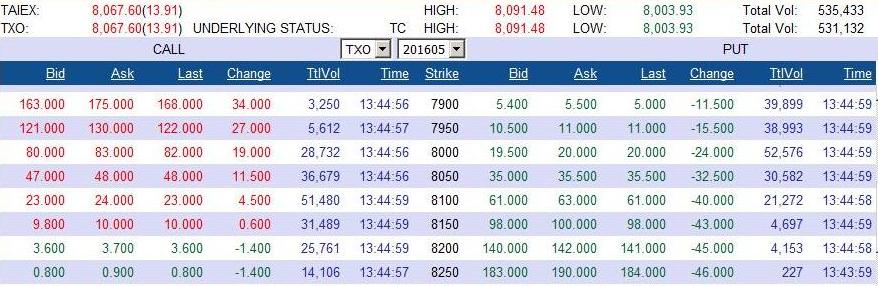
Fig. 1: Option Snapshot Quotes of the Taiwan Futures Exchange at May 16, 2016.

3 Data Collection and Processing

To address research question Q2 we apply the optimization problem (7)–(13) and construct the option’s strategy with the certain payoff function on the derivatives of Taiwan Futures Exchange. All options in the Taiwan’s market are European-style. The expiration periods of TXO options have spot month, the next two months, and the next two quarterly calendar months. We will be designing option’s portfolio from the daily closing ask- and bid-prices for TXO options. We select TXO options; they are liquid assets and comprise above $60\%$ of trading volume of TAIFEX. Here we have taken a single date, May 16, 2016, selected at random, to illustrate the portfolio design in practice.

The strikes and the ask- and bid-prices of options are required inputs to the portfolio optimization model. The available TXO prices are denominated in New Taiwan Dollars (NTD). The TAIFEX index closed at $8,067.60$ on May 16, 2016 (Fig. 1), and the May options contracts expired $9$ days later, on May 25, 2016. The option price equals to $S_{0}=8,067.60$ NTD at May 16, 2016. Next, we will consider two cases for the expected price, $\hat{S}_{T}$. Suppose that the price will significant move up to 1) $\hat{S}_{T}=8{,}300.00$ NTD, 2) $\hat{S}_{T}=8{,}400.00$ NTD at May 25, 2016.

The investor then wants to monetize his position, $C(t,X)=100$ NTD at the time of purchase, $t=0$, and to limit the maximum loss by $\mathcal{L}=-100$ NTD, if the price of underlying asset will come out of the certain range from $8{,}000$ to $8{,}400$ NTD, respectively. The margin requirement for short positions and transaction costs are not accounted.

Table 1: Optimal portfolios with the different initial costs, $C$, and the expected price $\hat{S}_{T}$, NTD

	$\hat{S}_{T}=8400$						$\hat{S}_{T}=8300$
Strike Price	$C=100$		$C=-100$		$C=0$		$C=100$		$C=-100$		$C=0$
	Call	Put	Call	Put	Call	Put	Call	Put	Call	Put	Call	Put
7850		0		0		0		0		0		0
7950		0		0		0		0		0		0
8050	4	-3	7	-6	3	-3	7	-7	3	-2	5	-5
8150	-8	8	-10	9	1	2	-8	9	-2	4	-4	6
8250	10	-5	4	0	-5	6	4	3	0	0	0	4
8350	-8	0	-3	-3	-5	-5	-3	-5	-1	-2	-5	-5
8400	-5		-2		2		-9		-7		-2
8500	7		4		4		9		7		6
$\max\limits_{X}\{F_{\mathcal{C}}(X)\}$	700		400		600		400		250		300
Total number of contracts	58		48		36		64		28		42

Table 2: Optimal portfolios with the different liquidity constraints, $|L|=U$, contracts, and the expected price $\hat{S}_{T}$, NTD

	$\hat{S}_{T}=8400$						$\hat{S}_{T}=8300$
Strike Price	$|L|=10^{a)}$		$|L|=50$		$|L|=100$		$|L|=10^{a)}$		$|L|=50$		$|L|=100$
	Call	Put	Call	Put	Call	Put	Call	Put	Call	Put	Call	Put
7850		0		0		0		0		0		0
7950		0		0		0		0		0		0
8050	4	-3	-24	24	-51	51	7	-7	-24	24	-50	50
8150	-8	8	50	-50	100	-100	-8	9	47	-47	100	-100
8250	10	-5	-11	30	-4	49	4	3	-4	22	-12	50
8350	-8	0	-27	-4	-89	0	-3	-5	-21	1	-40	0
8400	-5		-1		21		-9		-15		-35
8500	7		13		23		9		17		37
$\max\limits_{X}\{F_{\mathcal{C}}(X)\}$	700		1800		4400		400		800		1800
Total number of contracts	58		234		488		64		222		474
a) The column $|L|=10$ corresponds to the column $C=100$ of Table 1.

To establish the proposed strategy we use $12$ strike prices: sequential $n=6$ strike prices are corresponding to call

$$K_{c}=(\textbf{8050},8150,8250,8350,8400,8500)$$

and sequential $n=6$ strike prices are corresponding to put

$$K_{p}=(7850,7950,\textbf{8050},8150,8250,8350)$$

at the same expiration date May 25, 2016. The central strike of the option is $K=8050$, is marked with bold. The number of combinations of ask- and bid-price for the $12$ options equal to $2^{n}\times 2^{n}=2^{6}\times 2^{6}=4096$, thus the cardinality of set of feasible portfolios $|\mathcal{C}|=4096$. The cardinality of the set $|K|=|K_{p}\cup K_{c}|$ is $8$, therefore, we have $7$ pairs of sequential strike prices $[k_{q},k_{q+1}]$, and that these pairs produce the system of $7$ inequalities from Eq. (10), and we should add two equalities on the first closed interval and the left-closed interval from Eq. (8). In our example, we assumed that one can buy or sell at least $L=-10$, $U=10$ contracts at each strike price. This assumption does not limit our approach because the total volume (TtlVol, Fig. 1) is bigger for all strike prices. Then we calculate the price for call and put in accordance with the specific strike (Fig. 1). Next, we maximized the objective function $F_{\mathcal{C}}(X)$, proposed in Eq. (7) with the system of constraints (8)–(13). The optimal portfolio was obtained in approximately two minutes on a personal computer, using the MATLAB software.

As a result, the optimum solution in the case $\hat{S}_{T}=8400$, $C=100$ is

$$X=(\underbrace{4,-8,10,-8,5,7}_{\text{call}},\underbrace{0,0,-3,8,-5,0}_{\text{put}})$$

the first six elements correspond to call options, the second six – to put options, the total number of contracts are 58 out of which 34 are for buying and 24 are for selling, with objective function value equal to 700 NTD (bold in Table 1). The optimum solution in the case $\hat{S}_{T}=8300$, $C=100$ is

$$X=(\underbrace{7,-8,4,-3,-9,9}_{\text{call}},\underbrace{0,0,-7,9,3,-5}_{\text{put}})$$

– the total number of contracts are 64 out of which 32 are for buying and 32 are for selling, with objective function value equal to 400 NTD (bold in Table 1). From the Table 1 one can see that the maximum values of the payoff function are achieved at $C=100$ NTD, and the minimum values at $C=-100$ NTD.

At the end of the strategy term, May 25, 2016, the price of underlying index increased to $S_{T}=8{,}396.20$ NTD. The forecast come true, the amount of loss was limited by the maximal loss $\mathcal{L}=-100$.

3.1 The Sensitivity of the Solution to the Constraints Variation

The initial cost $C(t,X)$ Eq. (2) can be either a positive number or zero, or even negative number. We calculated the alternative portfolios with the different initial costs $C(t,X)=\{-100,0,100\}$ with fixed liquidity constraints $|L|=U=10$ Eq. (13), and then the values of liquidity constraints were varied $|L|=U=\{10,50,100\}$ with the fixed initial cost $C(t,X)=100$, results are represent in Tables 1, 2. Table 2 shows the strong dependence: with the increase in the number of liquidity constraints, i.e. $|L|=U$, the maximum value of the payoff function grows too.

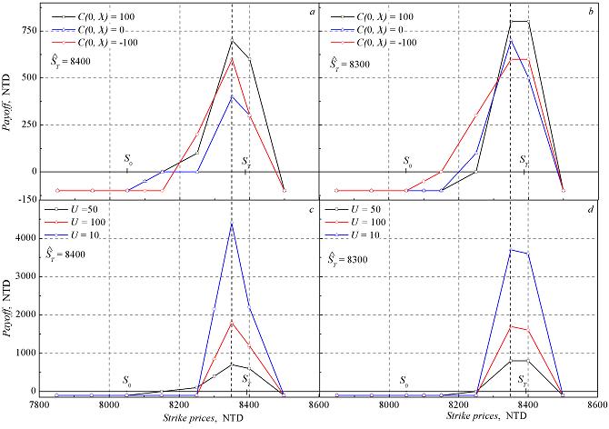
Fig. 2: Payoff functions of proposed option’s portfolios, underlying $S_{0}=8{,}067.60$ NTD. Different initial costs $C(t,X):100,0,-100$ NTD: a) $\hat{S}_{T}=8{,}400.00$ NTD, b) $\hat{S}_{T}=8{,}300.00$ NTD. Different liquidity constraints $L$, $U$, contracts: 10, 50, 100: c) $\hat{S}_{T}=8{,}400.00$ NTD, d) $\hat{S}_{T}=8{,}300.00$ NTD.

Fig. 2 show the payoff functions from the proposed option’s portfolio, taking into account, the different values of: a), b) the initial cost $C(t,X)$, Eq. (2) and c), d) liquidity constraints $L$, $U$, Eq. (13), respectively. Our strike prices are the $x$-axis and the payoff functions are the $y$-axis.

The expansion of the boundaries on the liquidity constraints $|L|=U\in\{10,50,100\}$ makes the options portfolio more attractive from the point of view of the terminal payoff amount. On the other hand, there is the difficulty of forming a strategy in view of the buy/sell of a sufficiently large number of underlying assets, a transaction which is difficult to implement for a short time.

4 Conclusion and Future Research

In this study, the description of the method of construction of the option’s strategy with the piecewise linear payoff function is carried out. We take into account the next set of assumptions of the proposed option’s strategy: strategy should effectively limit the upside earnings and downside risks; strategy should have an initial cost to enter; strategy should have protection on the downside and upside of the underlying asset price.

To address research question Q1 we have formulated the mathematical model as an integer linear programming problem which includes the system of constraints in the form of equalities and inequalities. The optimum solution was obtained using the MATLAB software.

To address research question Q2 we have demonstrated the possibility of the proposed model on the European-style TXO options of Taiwan Futures Exchange.

In the study we do not use the historical empirical distribution of returns. Our approach is statical, quite general and has the potential to design option’s portfolios on financial markets.

In option’s strategies, in addition to the forecast of the price of the underlying asset, various parameters can be taken into account: exercise price, volatility, the time to expiration, the risk-free interest rate, option premium, transaction costs. In this case, even an insignificant change of the parameter’s values can lead to a significant change in the number of possible combinations of option’s strategies. In our numerical experiments the total number of contracts for different cases varieties from 28 to 64 (Table 1) and from 58 to 488 (Table 2). In papers [14, 17, 18], it is noted that transactional costs in the dynamic management of the portfolio of options are one of the key factors without which it is impossible to talk about the feasibility of using the proposed models. The use of option strategies, including covered options, leads to deformation of the initial distribution of returns – it becomes truncated and asymmetric. The payoff of the option’s portfolio is asymmetric and non-linear, therefore, from the point of view of risk management. The use of a portfolio with various options contracts is preferable and effective, but the problem of choosing an optimal portfolio is significantly complicated too.

In this paper, we used the European type options in a series only. Pricing and valuation of the American option, even the single-asset option, is a hard problem in a quantitative finance [16, 19]. One of possible approach in the pricing and considering early exercise of the American option is dynamic programming.

The further research of our study can be continued in the following directions. At first, it is a portfolio optimization under transaction costs (exchange commissions, brokerage fees) and the margin requirement for short positions which are essential in the options market. At second, it is using options with different time to the expiration. At third, it is necessary to extend the system of constraints and add the budget constraint. Such extensions allows us to make the proposed approach more realistic and flexible.

5 Acknowledgments

Thanks to the editor and referees for several comments and suggestions that were instrumental in improving the paper. We are grateful to Dr. Sergey V. Kurochkin (National Research University Higher School of Economics, Russia) and Mr. Ashu Prakash (Indian Institute of Technology, Kanpur, India) for valuable comments and suggestions that improved the work and resulted in a better presentation of the material.

References

- [1] Bartonova, M. Hedging of sales by zero-cost collar and its financial impact [Text] / Marie Bartonova // Journal of Competitiveness. —2012. —Vol. 4, no. 2. —P. 111–127. —Access mode: http://www.cjournal.cz/files/99.pdf.
- [2] Kaur, A. Commodity hedging through zero-cost collar and its financial impact [Text] / Amandeep Kaur, Amandeep Singh Rattol // Journal of Energy and Management. —2016. —Vol. 1, no. 1. —P. 44–57. —Access mode: http://www.pdpu.ac.in/downloads/4.commodity_hedging.pdf.
- [3] Hull, J. Fundamentals of Futures and Options Markets [Text] / J.C. Hull. —New Jersey : Financial Times, 2002.
- [4] Ju, N. Options, option repricing in managerial compensation: Their effects on corporate investment risk [Text] / Nengjiu Ju, Hayne Leland, Lemma W. Senbet // Journal of Corporate Finance. —2013. —Access mode: http://dx.doi.org/10.1016/j.jcorpfin.2013.11.003.
- [5] A study of optimal stock and options strategies [Text] / M. Dash, V. Kavitha, K.M. Deepa, S. Sindhu // Social Science Research Network. —2007. —Access mode: http://dx.doi.org/10.2139/ssrn.1293203.
- [6] Garrett, S. An Introduction to the Mathematics of Finance. A Deterministic Approach [Text] / S.J. Garrett. —[S. l.] : Elsevier Ltd., 2013.
- [7] Griffin, B. Review of collar options for cotton industry [Text] / B. Griffin // Chemonics International Inc. —2007. —Access mode: http://pdf.usaid.gov/pdf{_}docs/PNADK976.pdf.
- [8] Ederington, L. Option spread and combination trading [Text]. —2002. —Access mode: http://optionsoffice.ru/wp-content/uploads/2013/08/Option-spread-combination-trading-{_}-Research-paper.pdf.
- [9] Carr, P. Towards a theory of volatility trading [Text] / P. Carr, D. Madan // Volatility: New Estimation Techniques for Pricing Derivatives / Ed. by R.A. Jarrow. —London : Risk Books, 1998. —P. 417–427.
- [10] Topaloglou, N. Optimizing international portfolios with options and forwards [Text] / N. Topaloglou, H. Vladimirou, S.A. Zenios // Journal of Banking and Finance. —2011. —Vol. 35. —P. 3188–3201.
- [11] Das, S. Options and structured products in behavioral portfolios [Text] / S.R. Das, M. Statman // Journal of Economic Dynamics and Control. —2013. —Vol. 37. —P. 137–153.
- [12] Kibzun, A. The two-step problem of investment portfolio selection from two risk assets via the probability criterion [Text] / A.I. Kibzun, A.N. Ignatov // Automation and Remote Control. —2015. —Vol. 76. —P. 1201–1220.
- [13] Lin, C.-C. Hedging an option portfolio with minimum transaction lots: A fuzzy goal programming problem [Text] / Chang-Chun Lin, Yi-Ting Liu, An-Pin Chen // Applied Soft Computing. —2016. —Vol. 47. —P. 295–303.
- [14] Davari-Ardakani, H. Multistage portfolio optimization with stocks and options [Text] / Hamed Davari-Ardakani, Majid Aminnayeri, Abbas Seifi // International Transactions in Operational Research. —2016. —Vol. 23, no. 3. —P. 593–622.
- [15] Moshenets, M. K. Automatic system of detecting informed trading activities in european-style options [Text] / M. K. Moshenets, O.L. Kritski // Journal of Engineering and Applied Sciences. —2016. —Vol. 11, no. 9. —P. 5727–5731.
- [16] Hajizadeh, E. Optimized radial basis function neural network for improving approximate dynamic programming in pricing high dimensional options [Text] / Ehsan Hajizadeh, Masoud Mahootchi // Neural Computing and Applications. —2016. —P. 1–12.
- [17] Goyal, A. Option returns and volatility mispricing [Text] / Amit Goyal, Alessio Saretto // Social Science Research Network. —2007. —Access mode: https://ssrn.com/abstract=889947.
- [18] Primbs, J. A. Dynamic hedging of basket options under proportional transaction costs using receding horizoncontrol [Text] / James A. Primbs // International Journal of Control. —2009. —Vol. 192, no. 3. —P. 1841–1855.
- [19] Mitchell, D. Boundary evolution equations for american options [Text] / D. Mitchell, J. Goodman, K Muthuraman // Math. Finance. —2014. —Vol. 24, no. 3. —P. 505?–532.