InferSpark: Statistical Inference at Scale

Abstract

The Apache Spark stack has enabled fast large-scale data processing. Despite a rich library of statistical models and inference algorithms, it does not give domain users the ability to develop their own models. The emergence of probabilistic programming languages has showed the promise of developing sophisticated probabilistic models in a succinct and programmatic way. These frameworks have the potential of automatically generating inference algorithms for the user defined models and answering various statistical queries about the model. It is a perfect time to unite these two great directions to produce a programmable big data analysis framework. We thus propose, InferSpark, a probabilistic programming framework on top of Apache Spark. Efficient statistical inference can be easily implemented on this framework and inference process can leverage the distributed main memory processing power of Spark. This framework makes statistical inference on big data possible and speed up the penetration of probabilistic programming into the data engineering domain.

1 Introduction

Statistical inference is an important technique to express hypothesis and reason about data in data analytical tasks. Today, many big data applications are based on statistical inference. Examples include topic modeling [5, 21], sentiment analysis [22, 13, 16], spam filtering [19], to name a few.

One of most critical steps of statistical inference is to construct a statistical model to formally represent the underlying statistical inference task [8]. The development of a statistical model is never trivial because a domain user may have to devise and implement many different models before finding a promising one for a specific task. Currently, most scalable machine learning libraries (e.g. MLlib [4]) only contain standard models like support vector machine, linear regression, latent Dirichlet allocation (LDA) [5], etc. To carry out statistical inference on customized models with big data, the user has to implement her own models and inference codes on a distributed framework like Apache Spark [26] and Hadoop [1].

Developing inference code requires extensive knowledge in both statistical inference and programming techniques in distributed frameworks. Moreover, model definitions, inference algorithms, and data processing tasks are all mixed up in the resulting code, making it hard to debug and reason about. For even a slight alteration to the model in quest of the most promising one, the model designer will have to re-derive the formulas and re-implement the inference codes, which is tedious and error-prone.

In this paper, we present InferSpark, a probabilistic programming framework on top of Spark. Probabilistic programming is an emerging paradigm that allows statistician and domain users to succinctly express a model definition within a host programming language and transfers the burden of implementing the inference algorithm from the user to the compilers and runtime systems [3]. For example, Infer.NET [17] is a probabilistic programming framework that extends C#. The user can express, say, a Bayesian network in C# and the compiler will generate code to perform inference on it. Such code could be as efficient as the implementation of the same inference algorithm carefully optimized by an experienced programmer.

So far, the emphasis of probabilistic programming has been put on the expressiveness of the languages and the development of efficient inference algorithms (e.g., variational message passing [24], Gibbs sampling [6], Metropolis-Hastings sampling [7]) to handle a wider range of statistical models. The issue of scaling out these frameworks, however, has not been addressed. For example, Infer.NET only works on a single machine. When we tried to use Infer.NET to train an LDA model of 96 topics and 9040-word vocabulary on only 3% of Wikipedia articles, the actual memory requirement has already exceeded 512GB, the maximum memory of most commodity servers today. The goal of InferSpark is thus to bring probabilistic programming to Spark, a predominant distributed data analytic platform, for carrying out statistical inference at scale. The InferSpark project consists of two parts:

• Extending Scala to support probabilistic programming

  Spark is implemented in Scala due to its functional nature. The fact that both preprocessing and post-processing can be included in one Scala program substantially eases the development process. In InferSpark, we extend Scala with probabilistic programming constructs to leverage its functional features. Carrying out statistical inference with InferSpark is simple and intuitive, and implicitly enjoys the distributed computing capability brought by Spark. As an example, the LDA statistical model was implemented using 503 lines of Scala code in MLlib (excluding comments, javadocs, blank lines, and utilities of MLlib). With InferSpark, we could implement that using only 7 lines of Scala code (see Figure 1).

• Building an InferSpark compiler and a runtime system

  InferSpark compiles InferSpark models into Scala classes and objects that implement the inference algorithms with a set of API. The user can call the API from their Scala programs to specify the input (observed) data and query about the model (e.g. compute the expectation of some random variables or retrieve the parameters of the posterior distributions).

⬇

1@Model

2class LDA(K: Long, V: Long, alpha: Double, beta: Double){

3 val phi = (0L until K).map{_ => Dirichlet(beta, K)}

4 val theta = ?.map{_ => Dirichlet(alpha, K)}

5 val z = theta.map{theta => ?.map{_ => Categorical(theta)}}

6 val x = z.map{_.map{z => Categorical(phi(z))}}

7}

Figure 1: Definition of Latent Dirichlet Allocation Model

Currently, InferSpark supports Bayesian network models. Bayesian network is a major branch of probabilistic graphical model and it has already covered models like naive Bayes, LDA, TSM [16], etc. The goal of this paper is to describe the workflow, architecture, and Bayesian network implementation of InferSpark. We will open-source InferSpark and support other models (e.g., Markov networks) afterwards.

To the best of our knowledge, InferSpark is the first endeavor to bring probabilistic programming into the (big) data engineering domain. Efforts like MLI [20] and SystemML [10] all aim at easing the difficulty of developing distributed machine learning techniques (e.g., stochastic gradient descent (SGD)). InferSpark aims at easing the complexity of developing custom statistical models, with statistician, data scientists, and machine learning researchers as the target users. This paper presents the following technical contributions of InferSpark so far.

• We present the extension of Scala’s syntax that can express various sophisticated Bayesian network models with ease.

• We present the details of compiling and executing an InferSpark program on Spark. That includes the mechanism of automatic generating efficient inference codes that include checkpointing (to avoid long lineage), proper timing of caching and anti-caching (to improve efficiency under memory constraint), and partitioning (to avoid unnecessary replication and shuffling).

• We present an empirical study that shows InferSpark can enable statistical inference on both customized and standard models at scale.

The remainder of this paper is organized as follows: Section 2 presents the essential background for this paper. Section 3 then gives an overview of InferSpark. Section 4 gives the implementation details of InferSpark. Section 5 presents an evaluation study of the current version of InferSpark. Section 6 discusses related work and Section 7 contains our concluding remarks.

2 Background

This section presents some preliminary knowledge about statistical inference and, in particular, Bayesian inference using variational message passing, a popular variational inference algorithm, as well as its implementation concerns on Apache Spark/GraphX stack.

2.1 Statistical Inference

Statistical inference is a common machine learning task of obtaining the properties of the underlying distribution of data. For example, one can infer from many coin tosses the probability of the coin turning up head by counting how many tosses out of the all tosses are head. There are two different approaches to model the number of heads: the frequentist approach and the Bayesian approach.

Let $N$ be the total number of tosses and $H$ be the number of heads. In frequentist approach, the probability of coin turning up head is viewed as an unknown fixed parameter so the best guess $\phi$ would be the number of heads $H$ in the results over the total number of tosses $N$.

$$\phi=\frac{H}{N}$$

In Bayesian approach, the probability of head is viewed as a hidden random variable drawn from a prior distribution, e.g., $\mathrm{Beta}(1,1)$, the uniform distribution over [0, 1]. According to the Bayes Theorem, the posterior distribution of the probability of coin turning up head can be calculated as follows:

$$p(\phi|x) =\frac{\phi^{H}(1-\phi)^{N-H}f(\phi;1,1)}{\int_{0}^{1}\phi^{H}(1-\phi)^{N-H}f(\phi;1,1)\mathrm{d}\phi}$$

$$=f(\phi;H+1,N-H+1)$$ (1)

where $f(\cdot;\alpha,\beta)$ is the probability density function (PDF) of $\mathrm{Beta}(\alpha,\beta)$ and $x$ is the outcome of $N$ coin tosses.

The frequentist approach needs smoothing and regularization techniques to generalize on unseen data while the Bayesian approach does not because the latter can capture the uncertainty by modeling the parameters as random variables.

2.2 Probabilistic Graphical Model

Probabilistic graphical model [14] (PGM) is a graphical representation of the conditional dependencies in statistical inference. Two types of PGM are widely used: Bayesian networks and Markov networks. Markov networks are undirected graphs while Bayesian networks are directed acyclic graphs. Each type of PGM can represent certain independence constraints that the other cannot represent. InferSpark currently supports Bayesian networks and regards Markov networks as the next step.

Figure 2: Bayesian network of the coin flip model (observed/unobserved random variable are in dark/white)

In a Bayesian network, the vertices are random variables and the edges represent the conditional dependencies between the random variables. The joint probability of a Bayesian network can be factorized into conditional probabilities of each vertex $\theta$ conditioned on their parents $\mathrm{F}(\theta)$. Figure 2 is the Bayesian network of the coin flip model. Here, the factors in the joint probability are $p(\phi)$ and $p(x|\phi)$. The plate surrounding $x$ represents repetition of the random variables. The subscript $N$ is the number of repetitions. The outcome of coin tosses $x$ is repeated $N$ times and each depends on the probability $\phi$. The Bayesian network of the coin flip model encodes the joint probability $p(\phi,x)=p(\phi)\prod_{i=1}^{N}p(x_{i}|\phi)$.

Bayesian networks are generative models, which describes the process of generating random data from hidden random variables. The typical inference task on generative model is to calculate the posterior distribution of the hidden variables given the observed data. In the coin flip model, the observed data are the outcomes of coin tosses and the hidden random variable is the probability of head. The inference task is to calculate the posterior in Equation 1.

2.3 Bayesian Inference Algorithms

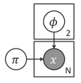
Figure 3: Bayesian network of the two-coin model

Inference of the coin flip model is simple because the posterior (Equation 1) has a tractable analytical solution. However, most real-world models are more complex than that and their posteriors do not have a familiar form. Moreover, even calculating the probability mass function or probability density function at one point is hard because of the difficulty of calculating the probability of the observed data in the denominator of the posterior. The probability of the observed data is also called evidence. It is the summation or integration over the space of hidden variables and is hard to calculate because of exponential growth of the number of terms.

Consider a two-coin model in Figure 3, where we first decide which coin to toss, with probability $\pi_{1}$ to choose the first coin and probability $\pi_{2}$ to choose the second coin ($\pi_{1}=1-\pi_{2}$). We then toss the chosen coin, which has probability $\phi_{i}$ to turn up head. This process is repeated $N$ times. The two-coin model is a mixture model, which represents the mixture of multiple sub-populations. Each such sub-population, in this case $\phi_{1}$ and $\phi_{2}$, have their own distributions, while the observation can only be obtained on the overall population, that is the number of heads after $N$ tosses. The two-coin model has no tractable analytical solution. Assuming Beta priors for $\pi$, $\phi_{1}$ and $\phi_{2}$, the posterior distribution is:

$$p(\pi,\phi|x)=\frac{p(\pi,\phi,x)}{\int p(\pi,\phi,x)\mathrm{d}\pi\mathrm{d}\phi_{1}\mathrm{d}\phi_{2}}$$

where the joint distribution $p(\pi,\phi,x)$ is:

$$f(\pi)f(\phi_{1})f(\phi_{2})(\pi_{1}\phi_{1}+\pi_{2}\phi_{2})^{H}(\pi_{1}(1-\phi_{1})+\pi_{2}(1-\phi_{2}))^{N-H}$$

The integral in the denominator of the posterior is intractable because it has $2^{N}$ terms and takes exponential time to compute. Since solving for the exact posterior is intractable, approximate inference algorithms are used instead. Although approximate inference is also NP-hard, it performs well in practical applications. Approximate inference techniques include Markov Chain Monte Carlo (MCMC) method, variational inference and so on. MCMC algorithms are inherently non-deterministic, and single random number generator is required to ensure randomness. In a distributed setting, sharing a single random number generator across the nodes in a cluster is a serious performance bottleneck. Having different generators on different nodes would risk the correctness of the MCMC algorithms. On the other hand, variational inference methods such as Variational Message Passing (VMP) [24] is a deterministic graph-based message passing algorithm, which can be easily adapted to a distributed graph computation model such as GraphX [25]. InferSpark currently supports VMP. Support of other techniques (e.g., MCMC) is included in InferSpark’s open-source agenda.

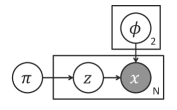
Figure 4: Expanded Bayesian network of the two-coin model

To infer the posterior of the two-coin model using VMP, the original Bayesian network has to be expanded by adding some more hidden random variables. Figure 4 shows Bayesian network with hidden random variables added, where $z_{i}$ is the index (1 or 2) of the coin chosen for the $i^{th}$ toss.

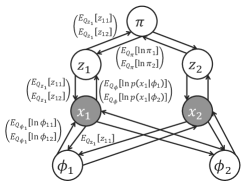
Figure 5: Message passing graph of the two-coin model

The VMP algorithm approximates the posterior distribution with a fully factorized distribution $Q$. The algorithm iteratively passes messages along the edges and updates the parameters of each vertex to minimize the KL divergence between $Q$ and the posterior. Because the true posterior is unknown, VMP algorithm maximizes the evidence lower bound (ELBO), which is equivalent to minimizing the KL divergence [24]. However, ELBO involves only the expectation of the log likelihoods of the approximated distribution $Q$ and is thus straightforward to compute.

Figure 5 shows the message passing graph of VMP for the two-coin model with $N=2$ tosses. There are four types of vertices in the two-coin model’s message passing graph: $\phi$, $\pi$, $z$, and $x$, with each type corresponding to a variable in the Bayesian network. Vertices in the Bayesian network are expanded in the message passing graph. For example, the repetition of vertex $\phi$ is 2 in the model. So, we have $\phi_{1}$ and $\phi_{2}$ in the massage passing graph. Edges in the two-coin model’s message passing graph are bidirectional and different messages are sent in different directions. The three edges $\pi\rightarrow z$, $z\rightarrow x$, $\phi_{k}\rightarrow x$ in the Bayesian network thus create six types of edges in the message passing graph: $\pi\rightarrow z_{i}$, $\pi\leftarrow z_{i}$, $z_{i}\rightarrow x_{i}$, $z_{i}\leftarrow x_{i}$, $\phi_{k}\rightarrow x_{i}$, and $\phi_{k}\leftarrow x_{i}$.

Each variable (vertex) is associated with the parameters of its approximate distribution. Initially the parameters can be arbitrarily initialized. For edges whose direction is the same as in the Bayesian network, the message content only depends on the parameters of the sender. For example, the message $m_{\pi\rightarrow z_{1}}$ from $\pi$ to $z_{1}$ is a vector of expectations of logarithms of $\pi_{1}$ and $\pi_{2}$, denoted as $\left(\hskip-5.0pt\begin{array}[]{r}E_{Q_{\pi}}[\ln\pi_{1}]\@arraycr E_{Q_{\pi}}[\ln\pi_{2}]\end{array}\hskip-5.0pt\right)$ in Figure 5. For edges whose direction is opposite of those in the Bayesian network, in addition to the parameters of the sender, the message content may also depend on other parents of the sender in the Bayesian network. For example, the message $m_{x_{1}\rightarrow z_{1}}$ from $x_{1}$ to $z_{1}$ is $\left(\hskip-5.0pt\begin{array}[]{r}E_{Q_{\pi}}[\ln p(x_{1}|\phi_{1})]\@arraycr E_{Q_{\pi}}[\ln p(x_{1}|\phi_{2})]\end{array}\hskip-5.0pt\right)$, which depends both on the observed outcome $x_{1}$ and the expectations of $\ln\phi_{1}$ and $\ln\phi_{2}$.

Based on the message passing graph, VMP selects one vertex $v$ in each iteration and pulls messages from $v$’s neighbor(s). If the message source $v_{s}$ is the child of $v$ in the Bayesian network, VMP also pulls message from $v_{s}$’s other parents. For example, assuming VMP selects $z_{1}$ in an iteration, it will pull messages from $\pi$ and $x_{1}$. Since $x$ is the child of $z$ in the Bayesian network (Figure 4), and $z$ depends on $\phi$, VMP will first pull a message from $\phi_{1}$ to $x_{1}$, then pull a message from $x_{1}$ to $z_{1}$. This process however is would not be propagated and is restricted to only $v_{s}$’s direct parents. On receiving all the requested messages, the selected vertex updates its parameters by aggregating the messages.

Implementing the VMP inference code for a statistical model (Bayesian network) $M$ requires (i) deriving all the messages mathematically (e.g., deriving $m_{x_{1}\rightarrow z_{1}}$) and (ii) coding the message passing mechanism specifically for $M$. The program tends to contain a lot of boiler-plate code because there are many types of messages and vertices. For the two-coin model, $x$ would be coded as a vector of integers whereas $z$ would be coded as a vector of probabilities (float), etc. Therefore, even a slight alteration to the model, say, from two-coin to two-coin-and-one-dice, all the messages have to be re-derived and the message passing code has to be re-implemented, which is tedious to hand code and hard to maintain.

2.4 Inference on Apache Spark

When a domain user has crafted a new model $M$ and intends to program the corresponding VMP inference code on Apache Spark, one natural choice is to do that through GraphX, the distributed graph processing framework on top of Spark. Nevertheless, the user still has to go through a number of programming and system concerns, which we believe, should better be handled by a framework like InferSpark instead.

First, the Pregel programming abstraction of GraphX restricts that only updated vertices in the last iteration can send message in the current iteration. So for VMP, when $\phi_{1}$ and $\phi_{2}$ (Figure 5) are selected to be updated in the last iteration (multiple $\phi$’s can be updated in the same iteration when parallelizing VMP), $x_{1}$ and $x_{2}$ cannot be updated in the current iteration unfortunately because they require messages from $z_{1}$ and $z_{2}$, which were not selected and updated in the last iteration. Working around this through the use of primitive aggregateMessages and outerJoinVertices API would not make life easier. Specifically, the user would have to handle some low level details such as determining which intermediate RDDs to insert to or evict from the cache.

Second, the user has to determine the best timing to do checkpointing so as to avoid performance degradation brought by the long lineage created by many iterations.

Last but not the least, the user may have to customize a partition strategy for each model being evaluated. GraphX built-in partitioning strategies are general and thus do not work well with message passing graphs, which usually possess (i) complete bipartite components between the posteriors and the observed variables (e.g., $\phi_{1}$, $\phi_{2}$ and $x_{1},\ldots,x_{N}$ in Figure 5), and (ii) large repetition of edge pairs induced from the plate (e.g., $N$ pairs of $\langle z_{i},x_{i}\rangle$ in Figure 5). GraphX adopts a vertex-cut approach for graph partitioning and a vertex would be replicated to multiple partitions if it lies on the cut. So, imagine if the partition cuts on $x$’s in Figure 5, that would incur large replication overhead as well as shuffling overhead. Consequently, that really requires the domain users to have excellent knowledge on GraphX in order to carry out efficient inference on Spark.

3 InferSpark Overview

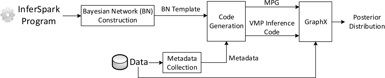
Figure 6: InferSpark Architecture

The overall architecture of InferSpark is shown in Figure 6. An InferSpark program is a mix of Bayesian network model definition and normal user code. The Bayesian network construction module separates the model part out, and transforms it into a Bayesian network template. This template is then instantiated with parameters and meta data from the input data at runtime by the code generation module, which produces the VMP inference code and message passing graph. These are then executed on the GraphX distributed engine to produce the final posterior distribution. Next, we describe the three key modules in more details with the example of the two-coin model (Figure 4).

3.1 Running Example

⬇

1@Model class TwoCoins(alpha: Double, beta: Double) {

2 val pi = Beta(alpha)

3 val phi = (0L until 2L).map(_ => Beta(beta))

4 val z = ?.map(_ => Categorical(pi))

5 val x = z.map(z => Categorical(phi(z)))

6}

7object Main {

8 def main() {

9 val xdata: RDD[Long] = /* load (observed) data */

10 val m = new TwoCoins(1.0, 1.0)

11 m.x.observe(xdata)

12 m.infer(steps=20)

13 val postPhi: VertexRDD[BetaResult] = m.phi.getResult()

14 /* postprocess */

15 ...

16 }

17}

Figure 7: Definition of two-coin model in InferSpark

Figure 7 shows the definition of the two-coin model in InferSpark. The definition starts with “@Model” annotation. The rest is similar to a class definition in scala. The model parameters (“alpha” and “beta”) are constants to the model. In the model body, only a sequence of value definitions are allowed, each defining a random variable instead of a normal deterministic variable. The use of “val” instead of “var” in the syntax implies the conditional dependencies between random variables are fixed once defined. For example, line 2 defines the random variable $\pi$ having a symmetric Beta prior $\mathrm{Beta}(\alpha,\alpha)$.

InferSpark model uses “Range” class in Scala to represent plates. Line 3 defines a plate of size 2 with the probabilities of seeing head in the two coins. The “?” is a special type of “Range” representing a plate of unknown size at the time of model definition. In this case, the exact size of the plate will be provided or inferred from observed variables at run time. When a random variable is defined by mapping from a plate of other random variables, the new random variable is in the same plate as the others. For example, line 5 defines the outcomes $x$ as the mapping from $z$ to Categorical mixtures, therefore $x$ will be in the same plate as $z$. Since the size of the plate surrounding $x$ and $z$ is unknown, we need to specify the size at run time. We can either explicitly set the length of the “?” or let InferSpark set that based on the number of observed outcomes $x$ (line 11).

At the first glance, “?” seems redundant since it can be replaced by a model parameter $N$ denoting the size of the plate. However, “?” becomes more useful when there are nested plates. In the two-coin model, suppose after we choose one coin, we toss it multiple times. Figure 8 shows this scenario. Then the outcomes $x$ are in two nested plates where the inner plate is repeated $M$ times, and each instance may have a different size $N_{i}$. Using the “?” syntax for the inner plate, we simply change line 5 to

Ψval x = z.map(z => ?.map(_ => Categorical(phi(z))))Ψ

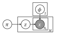
Figure 8: Two-coin Model with Nested Plates

3.2 Bayesian Network Construction

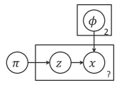
Figure 9: Bayesian Network Template Constructed from the Two-coin Model

An input InferSpark program is first parsed and separated into two parts: the model definition (“@Model class TwoCoins” in Figure 7) and the ordinary scala program (“object Main” in Figure 7). The model definition is analyzed and transformed into valid scala classes that define a Bayesian network constructed from the model definition (e.g., Figure 9) and the inference/query API. Note the Bayesian network constructed at this stage is only a template (different than Figure 4) because some of the information is not available until run time (e.g., the outcomes $x$, the number of coin flippings and the model parameters $\alpha$ and $\beta$).

3.3 Metadata Collection

Metadata such as the observed values and the plate sizes missing from the Bayesian networks are collected at runtime. In the two-coin model, an instance of the model is created via the constructor invocation (e.g. “val m = new TwoCoin(1.0, 1.0)” on line 10 of Figure 7). The constructor call provides the missing constants in the prior distributions of $\pi$ and $\phi$. For each random variable defined in the model definition, there is an interface field with the same name in the constructed object. Observed values are provided to InferSpark by calling the “observe” (line 11 of Figure 7) API on the field. There, the user provides an RDD of observed outcomes “xdata” to InferSpark by calling “m.x.observe(xdata)”. The observe API also triggers the calculation of unknown plate sizes. In this case, the size of plate surrounding $z$ and $x$ is automatically calculated by counting the number of elements in the RDD.

3.4 Code Generation

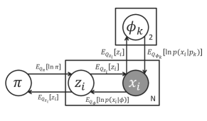
Figure 10: Bayesian Network with Messages for Two-coin Model

When the user calls “infer” API (line 12 of Figure 7) on the model instance, InferSpark checks whether all the missing metadata are collected. If so, it proceeds to annotate the Bayesian network with messages used in VMP, resulting in Figure 10. The expressions that calculate the messages (e.g., $E_{Q_{\pi}}[\ln\pi]$) depend on not only the structure of the Bayesian network and whether the vertices are observed or not, but also practical consideration of efficiency and constraints on GraphX.

To convert the Bayesian network to a message passing graph on GraphX, InferSpark needs to construct a VertexRDD and an EdgeRDD. This step generates the MPG construction code specific to the data. Figure 11 shows the MPG construction code generated for the two-coin model. The vertices are constructed by the union of three RDD’s, one of which from the data and the others from parallelized collections (lines 8 and line 9 in Figure 11). The edges are built from the data only. A partition strategy specific to the data is also generated in this step.

⬇

1class TwoCoinsPS extends PartitionStrategy {

2 override def getPartition /**/

3}

4def constrMPG() = {

5 val v1 = Categorical$13$observedValue.mapPartitions{

6 initialize z, x */

7 }

8 val v2 = sc.parallelize(0 until 2).map{ /* initialize phi */ }

9 val v3 = sc.parallelize(0 until 1).map{ /* initialize pi */ }

10 val e1 = Categorical$13$observedValue.mapParititons{

11 /* initialize edges */

12 }

13 Graph(v1 ++ v2 ++ v3, e1).partitionBy(new TwoCoinsPS())

14}

Figure 11: Generated MPG Construction Code

In addition to generating code to build the large message passing graph, the codegen module also generates code for VMP iterative inference. InferSpark, which distributes the computation, needs to create a schedule of parallel updates that is equivalent to the original VMP algorithm, which only updates one vertex in each iteration. Different instances of the same random variables can be updated at the same time. An example update schedule for the two-coins model is ($\pi$ and $\phi$) $\rightarrow$ $x$ $\rightarrow$ $z$ $\rightarrow$ $x$. VMP inference code that enforces the update schedule is then generated.

3.5 Getting the Results

The inference results can be queried through the “getResult” API on fields in the model instance that retrieves a VertexRDD of approximate marginal posterior distribution of the corresponding random variable. For example, in Line 13 of Figure 7, “m.phi.getResult()” returns a VertexRDD of two Dirichlet distributions. The user can also call “lowerBound” on the model instance to get the evidence lower bound (ELBO) of the result, which is higher when the KL divergence between the approximate posterior distribution and the true posterior is smaller.

⬇

1var lastL: Double = 0

2m.infer(20, { m =>

3 if ((m.roundNo > 1) ||

4 (Math.abs(m.lowerBound - lastL) <

5 Math.abs(0.001 * lastL))) {

6 false

7 } else {

8 lastL = m.lowerBound

9 true

10 }

11})

Figure 12: Using Callback function in “infer” API

The user can also provide a callback function that will be called after initialization and each iteration. In the function, the user can write progress reporting code based on the inference result so far. For example, this function may return false whenever the ELBO improvement is smaller than a threshold (see Figure 12) indicating the result is good enough and the inference should be terminated.

4 Implementation

The main jobs of InferSpark are Bayesian network construction and code generation (Figure 6). Bayesian network construction first extracts Bayesian network template from the model definition and transforms it into a Scala class with inference and query APIs at compile time. Then, code generation takes those as inputs and generates a Spark program that can generate the messaging passing graph with VMP on top. Afterwards, the generated program would be executed on Spark.

We use the code generation approach because it enables a more flexible API than a library. For a library, there are fixed number of APIs for user to provide data, while InferSpark can dynamically generate custom-made APIs according to the structure of the Bayesian network. Another reason for using code generation is that compiled programs are always more efficient than interpreted programs.

4.1 Bayesian Network Construction

In this offline compilation stage, the model definition is first transformed into a Bayesian network. We use the macro annotation, a compile-time meta programming facility of Scala. It is currently supported via the macroparadise plugin. After the parser phase, the class annotated with “@Model” annotation is passed from the compiler to its transform method. InferSpark treats the class passed to it as model definition and transforms it into a Bayesian network.

ModelDef	::=	‘@Model’ ‘class’ id
		‘(’ ClassParamsOpt ‘)’ ‘{’ Stmts ‘}’
ClassParamsOpt	::=	‘’ /* Empty */
	|	ClassParams
ClassParams	::=	ClassParam [‘,’ ClassParams]
ClassParam	::=	id ‘:’ Type
Type	::=	‘Long’ | ‘Double’
Stmts	::=	Stmt [[semi] Stmts]
Stmt	::=	‘val’ id = Expr
Expr	::=	‘{’ [Stmts [semi]] Expr ‘}’
	|	DExpr
	|	RVExpr
	|	PlateExpr
	|	Expr ‘.’ ‘map’ ‘(’ id => Expr ‘)’
DExpr	::=	Literal
	|	id
	|	DExpr (‘+’ | ‘-’ | ‘*’ | ‘/’) DExpr
	|	(‘+’ | ‘-’) DExpr
RVExpr	::=	‘Dirichlet’ ‘(’ DExpr ‘,’ DExpr ‘)’
	|	‘Beta’ ‘(’ DExpr ‘)’
	|	‘Categorical’ ‘(’ Expr ‘)’
	|	RVExpr RVArgList
	|	id
RVArgList	::=	‘(’ RVExpr ‘)’ [ RVArgList ]
PlateExpr	::=	DExpr ‘until’ DExpr
	|	DExpr ‘to’ DExpr
	|	‘?’
	|	id

Figure 13: InferSpark Model Definition Syntax

Figure 13 shows the syntax of InferSpark model definition. The expressions in a model definition is divided into 3 categories: deterministic expressions (DExpr), random variable expressions (RVExpr) and plate expressions. The deterministic expressions include literals, class parameters and their arithemetic operations. The random variable expressions define random variables or plates of random variables. The plate expressions define plate of known size or unknown size. The random variables defined by an expression can be binded to an identifier by the value definition. It is also possible for a random variable to be binded to multiple or no identifiers. To uniquely represent the random variables, we assign internal names to them instead of using the identifiers.

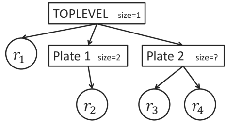
Figure 14: Internal Rep. of Bayesian Network

Internally, InferSpark represents a Bayesian network in a tree form, where the leaf nodes are random variables and the non-leaf nodes are plates. The edges in the tree represent the nesting relation between plates or between a plate and random variables. The conditional dependencies in the Bayesian network are stored in each node. The root of the tree is a predefined plate TOPLEVEL with size 1. Figure 14 is the internal representation of the two-coin model in Figure 9, where $r_{1}$, $r_{2}$, $r_{3}$, $r_{4}$, correspond to $\pi$, $\phi$, $z$, $x$, respectively. Plate 1 and Plate 2 correponds to the plates defined on lines 3–5 in Figure 7.

If a plate is nested within another plate, the inner plate is repeated multiple times, in which case, the size attribute of the plate node will be computed by summing the size of each repeated inner plate. We call the size attribute in the tree flattened size of a plate. For example, in Figure 8, the flattened size of the innermost plate around $x$ is $\sum_{i}N_{i}$.

InferSpark recursively descends on the abstract syntax tree (AST) of the model definition to construct the Bayesian network. In the model definition, InferSpark follows the normal lexical scoping rules. InferSpark evaluates the expressions to one of the following three results

• a node in the tree

• a pair $(r,\textrm{plate})$ where $r$ is a random variable node and plate is a plate node among its ancestors, which represents all the random variables in the plate

• a determinstic expression that will be evaluated at run time

At this point, apart from constructing the Bayesian network representation, InferSpark also generates the code for metadata collection, a module used in stage 2. For each random variable name bindings, a singleton interface object is also created in the resulting class. The interface object provides “observe” and “getResult” API for later use.

4.2 Code Generation

Code generation happens at run time. It is divided into 4 steps: metadata collection, message annotation, MPG construction code generation and inference execution code generation.

Metadata collection aims to collect the values of the model parameters, check whether random variables are observed or not, the flattened sizes of the plates. These metadata can help to assign VertexID to the vertices on the message passing graph. After the flattened sizes of plates are calculated, we can assign VertexIDs to the vertices that will be constructed in the message passing graph. Each random variable will be instantiated into a number of vertices on the MPG where the number equals to the flattened size of its innermost plate. The vertices of the same random variable are assigned consecutive IDs. For example, $x$ may be assigned ID from $0$ to $N-1$. The intervals of IDs of random variables in the same plate are also consecutive. A possible ID assignment to $z$ is $N$ to $2N-1$. Using this ID assignment, we can easily i) determine which random variable the vertex is from only by determining which interval the ID lies in; ii) find the ID of the corresponding random variable in the same plate by substracting or adding multiples of the flattened plate size (e.g. if $x_{i}$’ ID is $a$ then $z_{i}$’s ID is $a+N$).

Message annotation aims to annotate the Bayesian Network Template from the previous stage (Section 4.1) with messages to be used in VMP algorithm. The annotated messages are stored in the form of AST and will be incorporated into the the generated code, output of this stage. The rules of the messages to annotate are predefined according to the derivation of the VMP algorithm. After the messages are generated, we generate for each type of random variable a class with the routines for calculating the messages and updating the vertex.

The generated code for constructing the message passing graph requires building a VertexRDD and an EdgeEDD. The VertexRDD is an RDD of VertexID and vertex attribute pairs. Vertices of different random variables are from different RDDs (e.g., v1, v2, and v3 in Figure 11) and have different initialization methods. For unobserved random variables, the source can be any RDD that has the same number of elements as the vertices instantiated from the random variable. For observed random variables, the source must be the data provided by the user. If the observed random variable is in an unnested plate, the vertex id can be calculated by first combining the indices to the data RDD then adding an offset.

One optimization of constructing the EdgeRDD is to reverse the edges. If the code generation process generates an EdgeRDD in straightforward manner, the aggregateMessages function has to scan all the edges to find edges whose destinations are of $v$ type because GraphX indexes the source but not the destination. Therefore, when constructing the EdgeRDD, we generate code that reverses the edge so as to enjoy the indexing feature of GraphX. When constructing the graphs, we also take into account the graph partitioning scheme because that has a strong influence on the performance. We discuss this issue in the next section.

The final part is to generate the inference execution code that implements the iterative update of the VMP algorithm. We aim to generate code that updates each vertex in the message passing graph at least once in each iteration. As it is safe to update vertices that do not have mutual dependencies, i.e., those who do not send messages to one another, we divide each iteration into substeps. Each substep updates a portion of the message passing graph that does not have mutual dependencies.

A substep in each iteration consists of two GraphX operations: aggregateMessages and outerJoinVertices. Suppose g is the message passing graph, the code of a substep is:

⬇

1val prevg = g

2val msg = g.aggregateMessages(sendMsg, mergeMsg, TripletFields)

3g = g.outerJoinVertices(msg)(updateVertex).persist()

4g.edges.count()

5prevg.unpersist()

The RDD msg does not need to be cached because it is only used once. But the code generated has to cache the graph g because the graph is used twice in both aggregateMessages and outerJoinVertices. However, only caching it is not enough, the code generation has to include a line like 4 above to activate the caching process. Once g is cached, code generation evicts the previous (obsolete) graph prevg from the cache. To avoid the long lineage caused by iteratively updating message passing graph, which will overflow the heap space of the drive, the code generation process also adds a line of code to checkpoint the graph to HDFS every $k$ iterations.

4.3 Execution

The generated code at run time are sent to the Scala compiler. The resulting byte code are added to the classpath of both the driver and the workers. Then InferSpark initiates the inference iterations via reflection invocation.

4.4 Discussion on Partitioning Strategies

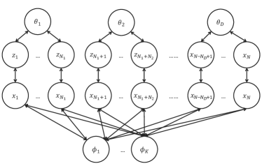
Figure 15: Message Passing Graph of a Mixture Model

GraphX adopts a vertex-cut partitioning approach. The vertices are replicated in edge partitions instead of edges being replicated in vertex partitions. The four built-in partition strategies in GraphX are: EdgePartition1D (1D), EdgePartition2D (2D), RandomVertexCut (RVC), and CanonicalRandomVertexCut (CRVC). In the following, we first show that these general partitioning strategies perform badly for the VMP algorithm on MPG. Then, we introduce our own partitioning strategy.

Figure 15 shows a more typical message passing graph of a mixture model instead of the toy two-coin model that we have used so far. $N$ is the number of $x$ and $z$, $K$ is the number of $\phi$, $D$ is the number of $\theta$. Typically, $N$ is very large because that is the data size (e.g., number of words in LDA), $K$ is a small constant (e.g., number of topics in LDA), and $D$ could be a constant or as large as $N$ (e.g., number of documents in LDA).

EdgePartition1D essentially is a random partitioning strategy, except that it co-locates all the edges with the same source vertex. Suppose all the edges from $\phi_{k}$ are assigned to partition $k$. Since there’s an edge from $\phi_{k}$ to each one of the $N$ vertices $x$, partition $k$ will have the replications of all $x_{1},x_{2},\ldots,x_{N}$. In the best case, edges from different $\phi_{k}$ are assigned to different partitions. Then the largest edge partition still have at least $N$ vertices. When $N$ is very large, the largest edge partition is also very large, which will easily cause the size of an edge partition to exceed the RDD block size limit. However, the best case turns out to be the worst case when it comes to the number of vertex replications because it actually replicates the size $N$ data $K$ times, which is extremely space inefficient. The over-replication also incurs large amount of shuffling when we perform outer joins because each updated vertex has to be shipped to every edge partition, prolonging the running time.

We give a more formal analysis of the number of vertices in the largest edge partition and the expected number of replications of $x_{i}$ under EdgePartition1D. As discussed above, there’s at least one edge partition that has replications of all the $x_{i}$’s. Observe that the graph has an upper bound of $3N+K$ vertices, so the number of vertices in the largest edge partition is $O(N)$. Let $N_{x_{i}}$ be the number of replications of $x_{i}$, then the expected number of replication of $x_{i}$ is

$$E[N_{x_{i}}] =M(1-(1-\frac{1}{M})^{K+1})$$

$$=\left\{\begin{array}[]{ll}(K+1)+o(1)&K=O(1)\\ M+o(1)&K=O(M)\end{array}\right.$$

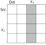
Figure 16: EdgePartition2D. Each grid is a partition. The possible partitions in which $x_{i}$ is replicated is shaded

EdgePartition2D evenly divides the adjacency matrix of the graph into $\sqrt{M}\times\sqrt{M}$ partitions. The vertices are uniformly distributed along the edges of the adjacency matrix by hashing into $\sqrt{M}$ buckets. The upper bound of the number of replications of a vertex $x_{i}$ is $\sqrt{M}$ because all the edges that point to it are distributed to at most $\sqrt{M}$ partitions in shown as Figure 16. Meanwhile, there are $K+1$ edges pointing to $x_{i}$, so the number of replications of $x_{i}$ cannot exceed $K+1$ as well. Therefore, the upper bound of replications of $x_{i}$ is actually $\min(K+1,\sqrt{M})$. On the other hand, suppose each of the $\phi_{k}$ is hashed to different bucket and $N$ $x$’s are evenly distributed into the $\sqrt{M}$ buckets, then the number of largest partition is at least $\frac{N}{\sqrt{M}}$, which is still huge when the average number of words per partition is fixed. Following is the formal analysis of the EdgePartition2D.

Let $B$ be an arbitrary partition in the dark column on Figure 16. Let $Y_{x_{i},B}$ be the indicator variable for the event that $x_{i}$ is replicated in Then the expectation of $Y_{x_{i},B}$ is

$$E[Y_{x_{i},B}] =1-(1-\frac{1}{\sqrt{M}})^{K+1}$$

The number of vertices $N_{B}$ in the largest partition $B$ is at least the expectation of the number of vertices in a partition, which is also at least the expectation of the number of $x_{i}$ in it:

$$E[N_{B}] =\sum_{v}E[Y_{v,B}]$$

$$\geq\frac{N}{\sqrt{M}}E[Y_{x_{i},B}]$$

$$=\left\{\begin{array}[]{ll}(K+1)\eta+o(1)&K=O(1)\\ \sqrt{M}\eta+o(1)&K=O(M)\end{array}\right.$$

The expected number of replications of $x_{i}$ is

$$E[N_{x_{i}}] =\sqrt{M}E[Y_{x_{i},B}]$$

$$=\left\{\begin{array}[]{ll}(K+1)+o(1)&K=O(1)\\ \sqrt{M}+o(1)&K=O(M)\end{array}\right.$$

RandomVertexCut (RVC) uniformly assigns each edge to one of the $M$ partitions. The expected number of replications of $x_{i}$ tends to be $O(K)$ when $K$ is a constant and tends to be $O(N)$ when $K$ is proportional to the number of partitions. The number of vertices in the largest partition is also excessively large. It is $O(K\frac{N}{M})$ when K is a constant and $O(N)$ when $K$ is proportional to the number of partitions. CanonicalRandomVertexCut assigns two edges between the same pair of vertices with opposite directions to the same partition. For VMP, it is the same as RandomVertexCut since only the destination end of an edge is replicated. For example, if $x_{i}$ has $K+1$ incoming edges, then the probability that $x_{i}$ will be replicated in a particular partition is independent from whether edges in opposite direction are in the same partition or randomly distributed. Therefore CRVC will have the same result as RVC. Table 1 and Table 2 summarize the comparison of different partition strategies.

InferSpark’s partitioning strategy is actually tailor-made for VMP’s message passing graph. The intuition is that the MPG has a special structure. For example, in Figure 15, we see that the MPG essentially has $D$ “independent” trees rooted at $\theta_{i}$, where the leaf nodes are $x$’s and they form a complete bipartite graph with all $\phi$’s. In this case, one good partitioning strategy is to form $D$ partitions, with each tree going to one partition and the $\phi$’s getting replicated $D$ times. We can see that such a partition strategy incurs no replication on $\theta$, $z$, and $x$, and incurs $D$ replications on $\theta$.

Generally, our partitioning works as follows: Given an edge, we first determine which two random variables (e.g. $x$ and $z$) are connected by the edge. It is quite straightforward because we assign ID to the set of vertices of the same random variable to a consecutive interval. We only need to look up which interval it is in and what the interval corresponds to. Then we compare the total number of vertices correponding to the two random variables and choose the larger one. Let the Vertex ID range of the larger one to be $L$ to $H$. We divide the range from $L$ to $H$ into $M$ subranges. The first subrange is $L$ to $L+\frac{H-L+1}{M}$; the second is $L+\frac{H-L+1}{M}+1$ to $L+2\frac{H-L+1}{M}$ and so on. If the vertex ID of the edge’s chosen vertex falls into the $m^{th}$ subrange, the edge is assigned to partition $m$.

In the mixture case, at least one end of every edge is $z$ or $x$. Since the number of $z$’s and $x$’s are the same, each set of edges that link to the $z_{i}$ or $x_{i}$ with the same $i$ are co-located. This guarantees that $z_{i}$ and $x_{i}$ only appears in one partition. All the $\phi_{k}$’s are replicated in each of the $M$ partitions as before. The only problem is that many $\theta_{j}$ with small $N_{j}$ could be replicated to the same location. In the worst case, the number of $\theta$ in one single partition is exactly $\eta$. However, it is not an issue in that case because the number of vertices in the largest partition is still a constant $3\eta+K$. It is also independent from whether $K=O(1)$ or $K=O(M)$.

Table 1: Analysis of Different Partition Strategies When $K=O(1)$

Partition Strategy	$E[N_{x_{i}}]$	$E[N_{B}]$
1D	$O(K)$	$O(N)$
2D	$O(K)$	$O(K\frac{N}{M})$
RVC	$O(K)$	$O(K\frac{N}{M})$
CRVC	$O(K)$	$O(K\frac{N}{M})$
InferSpark	1	$3\frac{N}{M}+1$

Table 2: Analysis of Different Partition Strategies When $K=O(M)$

Partition Strategy	$E[N_{x_{i}}]$	$E[N_{B}]$
1D	$O(M)$	$O(N)$
2D	$O(\sqrt{M})$	$O(\sqrt{M}\frac{N}{M})$
RVC	$O(M)$	$O(N)$
CRVC	$O(M)$	$O(N)$
InferSpark	1	$3\frac{N}{M}+1$

5 Evaluation

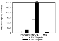
(a) LDA

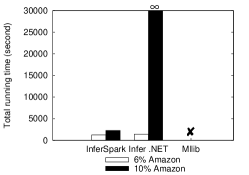
(b) SLDA

(c) DCMLDA

Figure 17: Running Time

In this section, we present performance evaluation of InferSpark, based on constructing and carrying out statistic inference on three models: Latent Dirichlet Allocation (LDA), Sentence-LDA (SLDA) [13], and Dirichlet Compound Multinomial LDA (DCMLDA) [9]. LDA is a standard model in topic modeling, which takes in a collection of documents and infers the topics of the documents. Sentence-LDA (SLDA) is a model for finding aspects in online reviews, which takes in online reviews, and infers the aspects. Dirichlet Compound Multinomial LDA (DCMLDA) is another topic model that accounts for burstiness in documents. All models can be implemented in InferSpark using less than 9 lines of code (see Figure 1 and Appendix A). For comparison, we include MLlib in our study whenever applicable. MLlib includes LDA as standard models. However, MLlib does not include SLDA and DCMLDA. There are other probabilistic programming frameworks apart from Infer.NET (see Section 6). All of them are unable to scale-out onto multiple machines yet. Infer.NET so far is the most predominant one with the best performance, so we also include it in our study whenever applicable.

All the experiments are done on nodes running Linux with 2.6GHz quad-core, 32GB memory, and 700GB hard disk. Spark 1.4.1 with scala 2.11.6 is installed on all nodes. The default cluster size for InferSpark and MLlib is 24 data nodes and 1 master node. Infer.NET can only use one such node. The data for running LDA, SLDA, and DCMLDA are listed in Table 3. The wikipedia dataset is the wikidump. Amazon is a dataset of Amazon reviews used in [13]. We run 50 iterations and do checkpointing every 10 iterations for each model on each dataset.

Table 3: Datasets

Wikipedia words topics 0.2% 541,644 96 0.5% 1,324,816 96 LDA	Amazon words topics 6% 349,569 96 10% 607,430 96 SLDA
Wikipedia words topics 0.5% 1,324,816 10 1% 2,596,155 10 DCMLDA

5.1 Overall Performance

Figure 17 shows the time of running LDA, SLDA, and DCMLDA on InferSpark, Infer.NET, and MLlib. Infer.NET cannot finish the inference tasks on all three models within a week. MLlib supports only LDA, and is more efficient than InferSpark in that case. However, we remark that MLlib uses the EM algorithm which only calculates Maximum A Posterior instead of the full posterior and is specific to LDA. In contrast, InferSpark aims to provide a handy programming platform for statistician and domain users to build and test various customized models based on big data. It would not be possible to be done by any current probabilistic frameworks nor with Spark/GraphX directly unless huge programming effort is devoted. MLlib versus InferSpark is similar to C++ programs versus DBMS: highly optimized C++ programs are more efficient, but DBMS achieves good performance with lower development time. From now on, we focus on evaluating the performance of InferSpark.

Table 4 shows the time breakdown of InferSpark. The inference process executed by GraphX, as expected, dominates the running time. The MPG construction step executed by Spark, can finish within two minutes. The Bayesian network construction and code generation can be done in seconds.

Table 4: Time Breakdown (in seconds and %)

Model	B.N. Construction		Code Generation		Execution				Total
					MPG Construction		Inference
LDA 541644 words	21.911	1.34%	11.15	0.68%	38.147	2.33%	1566.692	95.65%	1637.9
LDA 1324816 words	21.911	0.70%	12.25	0.39%	79.4	2.55%	3002.1	96.36%	3115.661
SLDA 349569 words	21.867	1.76%	11.05	0.89%	26.33	2.12%	1182.2	95.23%	1241.447
SLDA 607430 words	21.867	0.96%	11.69	0.52%	41.152	1.81%	2193.391	96.71%	2268.1
DCMLDA 1324816 words	22.658	0.65%	10.52	0.30%	20.923	0.60%	3448.699	98.46%	3502.8
DCMLDA 2596155 words	22.658	0.28%	11.55	0.14%	39.549	0.48%	8153.969	99.10%	8227.726

5.2 Scaling-Up

Figure 18 shows the total running time of LDA, SLDA, and DCMLDA on InferSpark by scaling the data size (in words). InferSpark scales well with the data size. DCMLDA exhibits even super-linear scale-up. This is because as the data size goes up, the probability of selecting larger documents goes up. Consequently, the growth in the total number of random variables is less than proportional, which gives rise to the super-linearity.

Figure 18: Scaling-up

5.3 Scaling-Out

Figure 19 shows the total running time of LDA on InferSpark in different cluster sizes. For each model, we use fixed size of dataset. DCMLDA and LDA both use the 2% Wikipedia dataset. SLDA uses the 50% amazon dataset. We observe that InferSpark can achieve linear scale-out.

Figure 19: Scaling-out

5.4 Partitioning Strategy

Figure 20 shows the running time of LDA(0.2% Wikipedia dataset, 96 topics) on InferSpark using our partitioning strategy and GraphX partitioning strategies: EdgePartition2D (2D) RandomVertexCut (RVC), CanonicalRandomVertexCut (CRVC), and EdgePartition1D (1D). We observe that the running time is propotional to the size of EdgeRDD. Our partition strategy yields the best performance for running VMP on the message passing graphs. Our analysis shows that RVC and CRVC should have the same results. The slight difference in the figure is caused by the randomness of different hash functions.

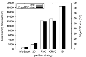
Figure 20: Comparison of Different Partition Strategies

6 Related Work

To the best of our knowledge, InferSpark is the only framework that can efficiently carry out statistical inference through probabilistic programming on a distributed in-memory computing platform. MLlib, Mahout [2], and MADLib [12] are machine learning libraries on top of distributed computing platforms and relational engines. All of them provide many standard machine learning models such as LDA and SVM. However, when a domain user, say, a machine learning researcher, is devising and testing her customized models with her big data, those libraries cannot help. MLBase [15] is related project that shares a different vision with us. MLBase is a suite of machine learning algorithms and provides a declarative language for users to specify machine learning tasks. Internally, it borrows the concept of query optimizer in traditional databases and has an optimizer that selects the best set of machine learning algorithms (e.g., SVM, Adaboost) for a specific task. InferSpark, on the other hand, goes for a programming language approach, which extends Scala with the emerging probabilistic programming constructs, and carries out statistical inference at scale. MLI [20] is an API on top of MLBase (and Spark) to ease the development of various distributed machine learning algorithms (e.g., SGD). In the same vein as MLI, SystemML [10] provides R-like language to ease the development of various distributed machine learning algorithms as well. In [23] the authors present techniques to optimize inference algorithms in a probabilistic DBMS.

There are a number of probabilistic programming frameworks other than Infer.NET [17]. For example, Church [11] is a probabilistic programming language based on the functional programming language Scheme. Church programs are interpreted rather than compiled. Random draws from a basic distribution and queries about the execution trace are two additional type of expressions. A Church expression defines a generative model. Queries of a Church expression can be conditioned on any valid church expressions. Nested queries and recursive functions are also supported by Church. Church supports stochastic-memoizer which can be used to express nonparametric models. Despite the expressive power of Church, it cannot scale for large dataset and models. Figaro is a probabilistic programming language implemented as a library in Scala [18]. It is similar to Infer .NET in the way of defining models and performing inferences but put more emphasis to object-orientation. Models are defined by composing instances of Model classes defined in the Figaro library. Infer.NET is a probabilistic programming framework in C# for Bayesian Inference. A rich set of variables are available for model definition. Models are converted to a factor graph on which efficient built-in inference algorithms can be applied. Infer.NET is the best optimized probabilistic programming frameworks so far. Unfortunately, all existing probabilistic programming frameworks including Infer.NET cannot scale out on to a distributed platform.

7 Conclusion

This paper presents InferSpark, a probabilistic programming framework on Spark. Probabilistic programming is an emerging paradigm that allows statistician and domain users to succinctly express a statistical model within a host programming language and transfers the burden of implementing the inference algorithm from the user to the compilers and runtime systems. InferSpark, to our best knowledge, is the first probabilistic programming framework that builts on top of a distributed computing platform. Our empirical evaluation shows that InferSpark can successfully express some known Bayesian models in a very succinct manner and can carry out distributed inference at scale. InferSpark will open-source. The plan is to invite the community to extend InferSpark to support other types of statistical models (e.g., Markov networks) and to support more kinds of inference techniques (e.g., MCMC).

8 Future Directions

Our prototype InferSpark system only implements the variational message passing inference algorithm for certain exponential-conjugate family Bayesian networks (namely mixtures of Categorical distributions with Dirichlet priors). In our future work, we plan to include support for other common types of Bayesian networks (e.g. those with continuous random variables or arbitrary priors). The VMP algorithm may be no longer applicable to these Bayesian networks because they may have non-conjugate priors or distributions out of exponential family. In order to handle wider classes of graphical models, we also plan to incorporate other inference algorithms (e.g. Belief propagation, Gibbs Sampling) into our system, which could be quite challenging because we have to 1) deal with arbitrary models 2) adapt the algorithm to distributed computing framework.

Another interesting future direction is to allow implementation of customized inference algorithms as plugins to the InferSpark compiler. To make the development of customized inference algorithms in InferSpark easier than directly writing them in a distributed computing framework, we plan to 1) revise the semantics of the Inferspark model definition language and expose a clean Bayesian network representation 2) provide a set of framework-independent operators for implementing the inference algorithms 3) investigate how to optimize the operators on Spark.

Appendix A SLDA and DCMLDA in InferSpark

⬇

1@Model

2class SLDA(K: Long, V: Long, alpha: Double, beta: Double) {

3 val phi = for (i <- 0L until K) yield Dirichlet(beta, V)

4 val theta = for (i <- ?) yield Dirichlet(alpha, K)

5 val z = theta.map{theta => for (i <- ?) yield Categorical(theta)}

6 val x = z.map(_.map(z => ?.map(_ => Categorical(phi(z)))))

7}

Figure 21: SLDA Model in InferSpark

⬇

1@Model

2class DCMLDA(K: Long, V: Long, alpha: Double, beta: Double) {

3 val doc = for (i <- ?) yield {

4 val phi = (0L until K).map(_ => Dirichlet(beta, V))

5 val theta = Dirichlet(alpha, K)

6 val z = ?.map(_ => Categorical(theta))

7 val x = z.map(z => Categorical(phi(z)))

8 }

9}

Figure 22: DCMLDA Model in InferSpark

References

- [1] Apache Hadoop. http://hadoop.apache.org/.
- [2] Apache Mahout. http://mahout.apache.org.
- [3] Probabilistic programming. http://probabilistic-programming.org/wiki/Home.
- [4] Spark MLLib. http://spark.apache.org/mllib/.
- [5] D. M. Blei, A. Y. Ng, and M. I. Jordan. Latent dirichlet allocation. JMLR, 3:993–1022, 2003.
- [6] W. Bolstad. Introduction to Bayesian Statistics. Wiley, 2004.
- [7] S. Chib and E. Greenberg. Understanding the metropolis-hastings algorithm. The American Statistician, 49(4):327–335, Nov. 1995.
- [8] D. R. Cox. Principles of statistical inference. Cambridge University Press, Cambridge, New York, 2006.
- [9] G. Doyle and C. Elkan. Accounting for burstiness in topic models. Icml, (Dcm):281–288, 2009.
- [10] A. Ghoting, R. Krishnamurthy, E. Pednault, B. Reinwald, V. Sindhwani, S. Tatikonda, Y. Tian, and S. Vaithyanathan. Systemml: Declarative machine learning on mapreduce. In Proceedings of the 2011 IEEE 27th International Conference on Data Engineering, ICDE ’11, pages 231–242, 2011.
- [11] N. D. Goodman, V. K. Mansinghka, D. M. Roy, K. Bonawitz, and J. B. Tenenbaum. Church: a language for generative models. In UAI, 2008.
- [12] J. M. Hellerstein, C. Ré, F. Schoppmann, D. Z. Wang, E. Fratkin, A. Gorajek, K. S. Ng, C. Welton, X. Feng, K. Li, and A. Kumar. The madlib analytics library: Or mad skills, the sql. Proc. VLDB Endow., 5(12):1700–1711, Aug. 2012.
- [13] Y. Jo and A. Oh. Aspect and Sentiment Unification Model for Online Review Analysis. In Proceedings of the fourth ACM international conference on Web search and data mining, 2011.
- [14] D. Koller and N. Friedman. Probabilistic graphical models: principles and techniques. 2009.
- [15] T. Kraska, A. Talwalkar, J. C. Duchi, R. Griffith, M. J. Franklin, and M. I. Jordan. Mlbase: A distributed machine-learning system. In CIDR, 2013.
- [16] Q. Mei, X. Ling, M. Wondra, H. Su, and C. Zhai. Topic sentiment mixture: modeling facets and opinions in weblogs. Proceedings of the 16th international conference on World Wide Web - WWW ’07, page 171, 2007.
- [17] T. Minka, J. Winn, J. Guiver, S. Webster, Y. Zaykov, B. Yangel, A. Spengler, and J. Bronskill. Infer.NET 2.6, 2014. Microsoft Research Cambridge. http://research.microsoft.com/infernet.
- [18] A. Pfeffer. Figaro: An object-oriented probabilistic programming language. Technical report, Charles River Analytics, 2009.
- [19] M. Sahami, S. Dumais, D. Heckerman, and E. Horvitz. A bayesian approach to filtering junk E-mail. In Learning for Text Categorization: Papers from the 1998 Workshop, Madison, Wisconsin, 1998. AAAI Technical Report WS-98-05.
- [20] E. R. Sparks, A. Talwalkar, V. Smith, J. Kottalam, X. Pan, J. E. Gonzalez, M. J. Franklin, M. I. Jordan, and T. Kraska. Mli: An api for distributed machine learning. In ICDM, pages 1187–1192, 2013.
- [21] I. Titov and R. McDonald. Modeling Online Reviews with Multi-grain Topic Models. 2008.
- [22] I. Titov, I. Titov, R. McDonald, and R. McDonald. A joint model of text and aspect ratings for sentiment summarization. Acl-08, 51(June):61801, 2008.
- [23] D. Z. Wang, M. J. Franklin, M. Garofalakis, J. M. Hellerstein, and M. L. Wick. Hybrid in-database inference for declarative information extraction. In Proceedings of the 2011 ACM SIGMOD International Conference on Management of Data, SIGMOD ’11, pages 517–528, New York, NY, USA, 2011. ACM.
- [24] J. M. Winn and C. M. Bishop. Variational message passing. In JMLR, pages 661–694, 2005.
- [25] R. S. Xin, J. E. Gonzalez, M. J. Franklin, and I. Stoica. Graphx: A resilient distributed graph system on spark. In GRADES ’13, pages 2:1–2:6.
- [26] M. Zaharia, M. Chowdhury, M. J. Franklin, S. Shenker, and I. Stoica. Spark: Cluster computing with working sets. In Proceedings of the 2Nd USENIX Conference on Hot Topics in Cloud Computing, HotCloud’10, pages 10–10, Berkeley, CA, USA, 2010. USENIX Association.