Constraints on the mass-richness relation from the abundance
and weak lensing of SDSS clusters

Abstract

We constrain the scaling relation between optical richness ($\lambda$) and halo mass ($M$) for a sample of SDSS redMaPPer galaxy clusters within the context of the Planck cosmological model. We use a forward modeling approach where we model the probability distribution of optical richness for a given mass, $P(\ln\lambda|M)$. To model the abundance and the stacked lensing profiles, we use an emulator specifically built to interpolate the halo mass function and the stacked lensing profile for an arbitrary set of halo mass and redshift, which is calibrated based on a suite of high-resolution $N$-body simulations. We apply our method to 8,312 SDSS redMaPPer clusters with $20\leq\lambda\leq 100$ and $0.10\leq z_{\lambda}\leq 0.33$, and show that the log-normal distribution model for $P(\lambda|M)$, with four free parameters, well reproduces the measured abundances and lensing profiles simultaneously. The constraints are characterized by the mean relation, $\left\langle\ln{\lambda}\right\rangle(M)=A+B\ln(M/M_{\rm pivot})$, with $A=3.207^{+0.044}_{-0.046}$ and $B=0.993^{+0.041}_{-0.055}$ (68% CL), where the pivot mass scale $M_{\rm pivot}=3\times 10^{14}h^{-1}M_{\odot}$, and the scatter $\sigma_{\mathrm{\ln\lambda}|M}=\sigma_{0}+q\ln(M/M_{\rm pivot})$ with $\sigma_{0}=0.456^{+0.047}_{-0.039}$ and $q=-0.169^{+0.035}_{-0.026}$. We find that a large scatter in halo masses is required at the lowest richness bins ($20\leq\lambda\lesssim 30$) in order to reproduce the measurements. Without such a large scatter, the model prediction for the lensing profiles tends to overestimate the measured amplitudes. This might imply a possible contamination of intrinsically low-richness clusters due to the projection effects. Such a low-mass halo contribution is significantly reduced when applying our method to the sample of $30\leq\lambda\leq 100$.

1. INTRODUCTION

The abundance of galaxy clusters is a powerful tool to constrain the primordial fluctuations as well as cosmological parameters: e.g., see White et al. (1993) for the pioneering theoretical work, Eke et al. (1996), Kitayama & Suto (1997) and Vikhlinin et al. (2009) for the cosmological constraints using the sample of X-ray clusters, Planck Collaboration et al. (2016b) for the sample of clusters selected via the Sunyaev-Zel’dovich (SZ) effect, and Rozo et al. (2010) for the sample of optically-selected clusters. In particular, the time evolution of the cluster abundance, if measured precisely, can be used to constrain properties of dark energy that govern the cosmic accelerating expansion (Haiman et al., 2001; Lima & Hu, 2005; Takada & Bridle, 2007; Oguri & Takada, 2011) (also see Weinberg et al., 2013, for a thorough review). Ongoing and upcoming wide-area galaxy surveys promise to further improve cluster-based cosmology, if systematic errors are under control. Such surveys include the Subaru Hyper Suprime-Cam (HSC) Survey (Aihara et al., 2017), the Dark Energy Survey, and ultimately the Large Synoptic Survey Telescope, the Euclid satellite mission, and the WFIRST satellite mission (Spergel et al., 2013).

The theoretical predictions for cluster observables are primarily given by the the halo mass for a given cosmological model. Therefore, to attain the full potential of cluster cosmology with upcoming wide-area surveys, we need to infer the “masses” of individual clusters or the average mass of a sample of clusters. In many cases we have to resort to mass-observable relations, which are calibrated by intensive observations of a subsample of clusters under consideration. Well-calibrated, unbiased mass-observable relations can allow us to infer the cluster masses on individual or statistical basis, thereby bridging the gap between theory and measurements and to obtain cosmological constraints from the comparison.

The weak gravitational lensing (Bartelmann & Schneider, 2001, for a review) has emerged as a powerful observable to constrain cluster masses. Gravitational lensing causes a coherent distortion pattern in the shapes of galaxies that lie in the background of galaxy clusters. Measurements of such distortions allow a direct measure of the projected mass density profile for the clusters, which in turn can be used to calibrate the cluster mass-observable relations (Johnston et al., 2007; Okabe et al., 2010, 2013; Hoekstra et al., 2015; van Uitert et al., 2016; Miyatake et al., 2016; Battaglia et al., 2016; Simet et al., 2017; Melchior et al., 2017). However, the weak lensing signal is too noisy to measure for individual clusters and is measurable only in a statistical sense, e.g., stacking shapes of many background galaxies for a sample of clusters. To obtain an unbiased estimation of the mass for the sampled clusters, we need to take into account the underlying distribution of clusters masses for the sample. In addition to this, the sample is usually affected by the measurement errors as well as intrinsic scatters in the mass-observable relation. These effects need to be carefully taken into account.

The main purpose of this paper is to calibrate the mass-observable relation from a joint measurement of the abundance (number counts) and the stacked cluster weak lensing profiles. We develop and apply our method to the SDSS redMaPPer cluster catalog that is constructed by identifying overdensities of red-sequence galaxies with similar colors as galaxy clusters from the SDSS $ugriz$ photometries (Rykoff et al., 2014; Rozo & Rykoff, 2014; Rozo et al., 2015a, b) (most recently Rykoff et al., 2016, for the details of the method). Since the cluster finder gives an estimation of the optical richness, $\lambda$, for each cluster, we will constrain the scaling relation between the optical richness and mass for the clusters. In this paper we develop a forward modeling approach, where we constrain the probability distribution of richness for a given halo mass, $P(\ln\lambda|M)$. This is in contrast with previous studies (Baxter et al., 2016; Simet et al., 2017; Melchior et al., 2017; Jimeno et al., 2017), where the backward modeling approach is employed to constrain the probability of mass for a given richness, $P(\ln M|\lambda)$. The forward modeling approach has several advantages. Firstly, we can use the abundance measurements more easily to constrain the mass-observable relation, as Saro et al. (2015) constrained $P(\ln\lambda|M)$ from the abundance measurements of SZ selected clusters after matching to redMaPPer clusters. Secondly, $P(\ln M|\lambda)$ can be inferred from $P(\ln\lambda|M)$ once the halo mass function $P(\ln M)$ is given, based on the Bayes theorem, while the opposite transformation, i.e, inferences of $P(\ln\lambda|M)$ from $P(\ln M|\lambda)$, is not straightforward, because this requires knowledge of the richness function $P(\ln\lambda)$ over the whole range of $\lambda$, which is not generally available, or is at least very noisy (and possibly affected by contamination), for richness below a threshold richness in cluster catalogs. Thirdly, the forward modeling is convenient to generate mock catalogs of clusters by populating halos in $N$-body simulations with galaxies, e.g. to test systematics in a cluster-finding algorithm.

In order to accurately constrain halo masses for a sample of the SDSS redMaPPer clusters, we need to properly model the mass density profile around the clusters for an assumed cosmological model (the Planck cosmological model (Planck Collaboration et al., 2016a) in our case). For this purpose we use a halo emulator, which is an interpolator for the halo mass function and the halo-matter cross-correlation function for an input set of parameters (halo mass, redshift, and correlation separation length or wavenumber). The emulator is built using a suite of high-resolution $N$-body simulations and their halo catalogs (Nishimichi et al. in prep.). The $N$-body simulation-calibrated emulator properly models both the 1-halo term, the 2-halo term and the transition regime of the mass profile, each of which is sensitive to the halo mass. In addition, the relation of halo concentration with mass, more generally variations in the halo profiles in the 1-halo regime, is automatically included in the emulator prediction. On the other hand, if an analytical model of the halo profile such as the Navarro-White-Frenk model (Navarro et al., 1996) is adopted, one needs to model the halo mass-concentration relation in order to compute the lensing profile, and such an analytical halo model ceases to be accurate at scales in the transition regime between the 1- and 2-halo terms, unless a sufficient number of free parameters are introduced (Diemer & Kravtsov, 2014). In order to model statistical errors in the abundance and the stacked lensing measured from the SDSS data over the survey footprint (about 10,000 ${\rm deg}^{2}$), we use 108 mock catalogs of the redMaPPer clusters and source galaxies for the entire SDSS footprint, which are generated based on the full-sky ray-tracing simulations and the resultant halo catalogs (Shirasaki et al., 2017; Takahashi et al., 2017). Thus we extensively use $N$-body simulation calibrated models and mocks in preparation for high-precision cosmology with cluster observables that will become available with upcoming surveys. Although we apply this method to the SDSS redMaPPer clusters, it is applicable to any cluster sample including the high-redshift cluster catalog that is built based on the deep Subaru HSC data (Oguri et al., 2017).

This paper is organized as follows. In Section 2, we describe details of cluster observables we measure from the SDSS data: the cluster abundance and the stacked lensing profile. In Section 3, we introduce a model to describe the mass-richness relation, $P(\ln\lambda|M)$, and then formulate the method to model the cluster observables in a forward modeling approach way, where all the observables in a given richness bin are modeled from $P(\ln\lambda|M)$ for an assumed cosmology. In Section 4.1, we describe the halo emulator to model the lensing profile and the halo mass function for the Planck cosmology, and then, in Section 4.2, describe details of the mock catalogs of the SDSS data which are used to estimate the error covariance matrix for the cluster observables. In Section 5, we show the results obtained by applying the method to the SDSS data, which include constraints on the mass-richness relation, and compare our results with previous work in Simet et al. (2017). In Section 6, we discuss the impact of possible residual systematic errors on our results. Section 7 is devoted to conclusion and summary. Throughout this paper we use natural units in which the speed of light is set equal to one, $c=1$. We adopt $M\equiv M_{\rm 200m}=4\pi(R_{200{\rm m}})^{3}\bar{\rho}_{\rm m0}\times 200/3$ for the halo mass definition, where $R_{\rm 200m}$ is the spherical halo boundary radius within which the mean mass density is $200$ times the present-day mean mass density. As for the fiducial cosmological model, we adopt the Planck cosmology (Planck Collaboration et al., 2016a): $\Omega_{\rm b0}h^{2}=0.02225$ and $\Omega_{\rm c0}h^{2}=0.1198$ for the density parameters of baryon and cold dark matter, respectively, $\Omega_{\Lambda}=0.6844$ for the cosmological constant, and $\ln(10^{10}A_{s})=3.094$ and $n_{s}=0.9645$ for the primordial power spectrum.

2. DATA AND CLUSTER OBSERVABLES

In this section we describe details of the data and cluster observables used in this paper: the abundance and stacked cluster lensing.

2.1. The SDSS redMaPPer cluster catalog

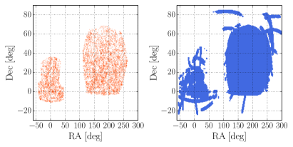
We use the catalog of galaxy clusters identified from the SDSS DR8 photometric galaxy catalog (Aihara et al., 2011) by the red-sequence Matched-filter Probabilistic Percolation (redMaPPer) cluster finder algorithm of v6.3 (Rykoff et al., 2014; Rozo et al., 2015b; Rykoff et al., 2016). We also refer to the website for further details. The cluster finder uses the SDSS $ugriz$ magnitudes and their errors to identify overdensities of red-sequence galaxies with similar colors. For each cluster, the catalog contains an optical richness estimate $\lambda$, a photometric redshift $z_{\lambda}$, the angular position and centering probabilities of five candidate central galaxies. Throughout this paper we use the position of the most probable central galaxy in each cluster region as a proxy of the cluster center. We denote the centering probability for the chosen central galaxy in each cluster region by $p_{\rm cen}$. A separate member galaxy catalog provides a list of members for each cluster, with assigned membership probability, $p_{\mathrm{mem}}$. The typical photometric redshift error, $\sigma(z_{\lambda})$, has been shown to be of order 0.01 (Rykoff et al., 2016). In addition, the typical richness estimate error, $\sigma(\lambda)$, is about $3$. Following Miyatake et al. (2016), in this paper we adopt the parent cluster catalog consisting of 8,312 redMaPPer clusters with $20\leq\lambda\leq 100$ and $0.10\leq z_{\lambda}\leq 0.33$, which is an approximately volume-limited sample (also see More et al., 2016). The average and median redshift of the clusters are $0.24$ and $0.25$, respectively. We assume $\Omega_{\mathrm{tot}}=10,401\ \mathrm{deg}^{2}$ for the total survey area which takes into account the cut of contiguous high-quality data based on the masks defined in the BOSS analysis (Dawson et al., 2013), compared to the original DR8 imaging catalog covering approximately $14,000~{}$deg² (see Section 2.2 in Rykoff et al., 2016, for details). Figure 1 shows the SDSS survey footprint, where the redMaPPer clusters are defined.

The optical richness $\lambda$ for each cluster is estimated as the sum of membership probability $p_{\mathrm{mem}}$ for all the potential member galaxies, as described in Rozo et al. (2009) and Rykoff et al. (2012):

$$\frac{\lambda}{S}=\sum_{\mathrm{gals}}p_{\mathrm{mem}},$$ (1)

where $S$ is a scale factor to correct for the effects of masks and depth variation on optical richness estimation.

Since a cluster is a finite size object and the projected size depends on richness and redshift of a cluster, a detection efficiency of the cluster depends on the richness and redshift as well as observational effects such as the survey boundary and masked regions. The redMaPPer finding algorithm adopts a richness-dependent, circular aperture to estimate the richness for each cluster (Rykoff et al., 2012; Rozo et al., 2015b):

$$R_{\rm aperture}(\lambda,z)=1.0\times\left(\frac{\lambda}{100}\right)^{0.2}(1+z)~{}~{}[h^{-1}{\rm Mpc}],$$ (2)

in comoving coordinates. In order to estimate the most probable richness for each cluster, the richness is iteratively determined by varying the aperture size.

To measure the stacked cluster lensing profiles, we use 120 times larger number of random points (therefore one million points) than the number of clusters in our samples, which was defined in Rykoff et al. (2016). These random points incorporate the survey geometry, depth variations (hence the detection rate of a cluster), and distributions of clusters in redshift and richness; accordingly each random point has the assigned richness and redshift from the clusters in the real catalog. Furthermore, Rykoff et al. (2016) used the random catalog to estimate a detection efficiency for each cluster with $\lambda$ and $z_{\lambda}$:

$$w_{\mathrm{rand}}(\lambda,z_{\lambda})=\frac{n_{\rm samp}(\lambda,z_{\lambda})}{n_{\rm keep}(\lambda,z_{\lambda})}.$$ (3)

Here $n_{\rm samp}(\lambda,z_{\lambda})\sim 1000$ is the total number of random points, which are injected into the survey footprint, for each of the clusters (here the cluster with $(\lambda,z_{\lambda})$), and $n_{\rm keep}(\lambda,z_{\lambda})$ is the number of the random points that pass the mask and richness threshold cuts, $f_{\rm mask}\leq 0.2$ and $\lambda/S\geq 20$, where $f_{\rm mask}$ is the weighted area fraction of masks within the aperture around the chosen position. The detection efficiency is given by $1/w_{\rm rand}$ and has a lower value for lower richness clusters, because such clusters are more affected by the survey boundary, masks and depth variations. We can use this to estimate an effective area for clusters with $\lambda$ and $z_{\lambda}$:

$$\Omega_{\rm eff}(\lambda,z_{\lambda})=\frac{\Omega_{\rm tot}}{w_{\rm rand}(\lambda,z_{\lambda})},$$ (4)

where $\Omega_{\rm eff}(\lambda,z_{\lambda})\leq\Omega_{\rm tot}$.

Figure 1.— Left: The distribution of SDSS redMaPPer clusters in the celestial coordinates, where each dot corresponds to a cluster (Rykoff et al., 2016). We use $8,312$ clusters with richness and redshift range of $20\leq\lambda\leq 100$ and $0.10\leq z_{\lambda}\leq 0.33$, which makes the sample nearly volume-limited, over the total area of $\Omega_{\rm tot}=10,401~{}\mathrm{deg^{2}}$. Right: The distribution of galaxies in the SDSS shape catalog, used for the stacked lensing analysis, taken from Mandelbaum et al. (2013). There are approximately 39 million source galaxies used for the lensing analysis in this paper, which have a slightly different distribution from that of the redMaPPer clusters based on the different cuts of the data (image quality and depth). For illustrative purpose, we show the distribution after assigning the source galaxies to rectangular pixels in the RA and Dec coordinates.

2.2. Cluster abundance

Table 1Binning scheme for the redMaPPer clusters and characteristics in each bin

bin index (abundance)	bin index (lensing)	$\lambda_{\mathrm{min}}$	$\lambda_{\mathrm{max}}$	$\left<\lambda\right>$	$z_{\mathrm{min}}$	$z_{\mathrm{max}}$	$\left<z_{\lambda}\right>$	$\left<p_{\mathrm{cen}}\right>$	$N^{\rm raw}_{\lambda_{\alpha}}$	$N^{\rm corr}_{\lambda_{\alpha}}$
1	1	20.0	25.0	22.3	0.10	0.33	0.25	0.87	3133	3488.4 (11.3%)
2	1	25.0	30.0	27.2	0.10	0.33	0.24	0.86	1762	1790.8 (1.6%)
3	2	30.0	35.0	32.3	0.10	0.33	0.24	0.86	1146	1164.1 (1.6%)
4	2	35.0	40.0	37.4	0.10	0.33	0.24	0.86	734	745.7 (1.6%)
5	3	40.0	47.5	43.5	0.10	0.33	0.24	0.87	596	605.2 (1.5%)
6	3	47.5	55.0	51.0	0.10	0.33	0.24	0.88	381	386.8 (1.5%)
7	4	55.0	77.5	63.6	0.10	0.33	0.24	0.87	434	440.4 (1.5%)
8	4	77.5	100	85.8	0.10	0.33	0.23	0.89	126	127.8 (1.4%)

Note. — In this paper we use the abundance and lensing measurements in eight and four richness bins, respectively, where each richness bin is defined by $\lambda_{\rm min}$ and $\lambda_{\rm max}$ as denoted in the third and fourth columns. For the redshift range, we use the same cut, $0.10\leq z_{\lambda}\leq 0.33$ for all the bins. The fifth and eighth columns give the mean richness and the mean redshift of the clusters in each richness bin. The ninth column gives the mean of the centering probability of the chosen central galaxies in each sample. The tenth column shows the number of clusters, and the eleventh shows the number after correcting for the effective survey area due to the effects of survey boundary and masks according to equation (5). The number in parenthesis in the eleventh column shows the ratio of the abundances before and after the correction.

As the first cluster observable, we consider the abundance of redMaPPer clusters, the total number of clusters observed across the entire SDSS footprint in a given richness bin. Throughout this paper, we use a single redshift bin, i.e. $0.10\leq z_{\lambda}\leq 0.33$, and do not consider smaller bins in redshift. Instead we divide the clusters into eight richness bins, as given in Table 1. In addition, we use the point estimate of richness and redshift for the clusters to calculate the abundance in this section and lensing profile in Section 2.3.

We use the abundance of the clusters in each richness bin correcting for the detection efficiency:

$$\widehat{N}_{\lambda_{\alpha}}=\sum_{l;{\lambda_{l}\in\lambda_{\alpha}}}\frac{\Omega_{\rm tot}}{\Omega_{\rm eff}(z_{l},\lambda_{l})},$$ (5)

where $\lambda_{\alpha}$ denotes the $\alpha$-th richness bin in Table 1, and the summation runs over all the clusters residing in the richness bin. The factor $\Omega_{\rm tot}/\Omega_{\rm eff}$ corrects for the detection efficiency we discussed. Equation (5) gives an estimator of the abundance of the clusters we could observe under the perfect conditions for the survey area of $\Omega_{\rm tot}$, i.e. the abundance without masking and depth-variation effects. With this correction, we need not consider the effects of survey boundary and masks on the model prediction. The number of clusters in the $\alpha$-th richness bin before and after the detection efficiency correction are given by $N_{\lambda_{\alpha}}^{\rm raw}$ and $N_{\lambda_{\alpha}}^{\rm corr}$, respectively, in Table 1. The correction is larger for a lower richness bin; the correction is about 11% for the lowest richness bin ($20\leq\lambda\leq 25$). In order to study the impact of the lowest richness bin on our results, in what follows, we will consider two samples defined by $20\leq\lambda\leq 100$ and $30\leq\lambda\leq 100$, respectively, and compare the results.

2.3. Stacked cluster lensing

The cross-correlation of positions of the redMaPPer clusters with shapes of background galaxies allows us to measure the average excess mass density profile around the clusters – hereafter the stacked cluster lensing profile. We use the catalog of source galaxy shapes in Mandelbaum et al. (2013) (also see Reyes et al., 2012), constructed after the carefully-tuned selection based on the imaging quality, data reduction quality, galactic extinction, apparent magnitude, photometric redshift and galaxy size. We use approximately the 39 million source galaxies. The area coverage is approximately $9,000~{}\mathrm{deg^{2}}$ and the footprint is overlapped with that of the redMaPPer catalog on the sky as shown in Figure 1.

The galaxy shapes in this catalog are measured using the re-Gaussianization technique (Hirata & Seljak, 2003), and the systematic uncertainties on shape measurements have been investigated in detail (Mandelbaum et al., 2005). Following Mandelbaum et al. (2013), we use the photometric redshift derived from a template-fitting method; the Zurich Extragalactic Bayesian Redshift Analyzer, or $\mathtt{ZEBRA}$ (Feldmann et al., 2006). For each galaxy, we use the best-fitting photometric redshift estimate after marginalizing over the SED templates. We correct for a bias in the lensing signal due to the photometric redshift errors by using the method in Nakajima et al. (2012). For the redshift binning ($0.10\leq z_{\lambda}\leq 0.33$), the debias factor is found to be about $1.08$ for all the richness bins, and we applied these correction factors for all the lensing signals.

To estimate the excess surface mass density profile for a sample of redMaPPer clusters in a given richness bin, we use the estimator defined in Mandelbaum et al. (2013):

$$\widehat{\Delta\Sigma_{\lambda_{\beta}}}(R) = \frac{1}{2\mathcal{R}}\left[\frac{1}{N_{ls,\beta}(R)}\left.\sum_{l,s;\lambda_{l}\in\lambda_{\beta}}w_{ls}\Sigma_{\rm cr}(z_{l},z_{s})\epsilon_{+}({\boldsymbol{\theta}}_{s})\right|_{R=\chi_{l}|\boldsymbol{\theta}_{l}-\boldsymbol{\theta}_{s}|}\right.$$

$$\left.-\frac{1}{N_{rs,\beta}(R)}\left.\sum_{r,s;\lambda_{r}\in\lambda_{\beta}}w_{rs}\Sigma_{\rm cr}(z_{r},z_{s})\epsilon_{+}({\boldsymbol{\theta}}_{s})\right|_{R=\chi_{r}|\boldsymbol{\theta}_{r}-\boldsymbol{\theta}_{s}|}\right],$$

where the index $\beta$ denotes the $\beta$-th richness bin as given in Table 1, the subscripts $s,l$ or $r$ stand for source, lens (cluster) or random, and $\epsilon_{+}$ is the tangential component of source galaxy ellipticity with respect to the cluster center or the random point. The shear responsivity (Bernstein & Jarvis, 2002) is given as $\mathcal{R}\simeq 0.87$ (Mandelbaum et al., 2013), which represents the statistically-averaged response of galaxy ellipticities to the lensing shear in the weak lensing regime. The summation runs over all pairs of source galaxies and clusters (or randoms) in a given projected separation $R=\chi_{l}|\boldsymbol{\theta}_{l}-\boldsymbol{\theta}_{s}|$ (or $R=\chi_{r}|\boldsymbol{\theta}_{r}-\boldsymbol{\theta}_{s}|$) to within the bin width, where $\chi_{l}\equiv\chi(z_{l})$ (or $\chi_{r}\equiv\chi(z_{r})$) is the comoving angular diameter distance to each cluster (or random). As given in Table 1, we divide the redMaPPer clusters into four richness bins, where we adopt a binning scheme similar to that in Simet et al. (2017) to enable comparison to their work. We use 19 radial bins that are equally spaced logarithmically from $0.2\ h^{-1}\mathrm{Mpc}$ to $50\ h^{-1}\mathrm{Mpc}$. The lensing efficiency function is defined for a system of lens and source at $z_{l}$ and $z_{s}$ for a flat universe as

$$\Sigma_{\rm cr}^{{{\color[rgb]{0,0,0}-1}}}(z_{l},z_{s})=4\pi G(1+z_{l})\chi_{l}\left(1-\frac{\chi_{l}}{\chi_{s}}\right).$$ (7)

The second term in equation (LABEL:eq:DSigma_est) denotes the lensing signals around the random points. As stressed in Sheldon et al. (2004) and Mandelbaum et al. (2005) (also see Singh et al., 2017, for a recent detailed study), the subtraction of the random signal from the signals around the clusters (the first term) allows us to measure the excess mass density profile around the clusters with respect to the background density. The random subtraction can also correct for an additive bias in the estimated shear e.g. due to PSF ellipticity errors (Mandelbaum et al., 2005). For a given subsample of the clusters, we use those random points, which fall in the same richness and redshift bins, to estimate the random signal. The lens-source pair weight $w_{ls}$ is given as

$$w_{ls}=\frac{\Omega_{\rm tot}}{\Omega_{\rm eff}(z_{l},\lambda_{l})}\Sigma^{{{\color[rgb]{0,0,0}-2}}}_{\mathrm{cr}}(z_{l},z_{s})w_{s},$$ (8)

where $w_{s}$ is the source weight as

$$w_{s}=\frac{1}{\sigma_{e}^{2}+\sigma_{\rm SN}^{2}},$$ (9)

where $\sigma_{e}$ is the measurement error of galaxy ellipticity and $\sigma_{\rm SN}$ is the intrinsic ellipticity amplitude, for which we used a fixed value, $\sigma_{\rm SN}=0.365$ following Reyes et al. (2012). The factor of $\Omega_{\rm eff}(\lambda_{l},z_{l})/\Omega_{\rm tot}$ in equation (8) corrects for the effective area as we did for the abundance estimator in equation (5). Similarly, the weight $w_{rs}$ for the random points is given as

$$w_{rs}=\left(\frac{\Omega_{\rm tot}}{\Omega_{\rm eff}(z_{r},\lambda_{r})}\right)^{2}\Sigma^{{{\color[rgb]{0,0,0}-2}}}_{\mathrm{cr}}(z_{r},z_{s})w_{s}.$$ (10)

The extra factor $\Omega_{\rm tot}/\Omega_{\rm eff}$ in this weight is from the fact that the number of random points in each richness bin accounts for the detection efficiency in the construction as described around equation (3). Note that, although the richness and redshift distributions of the original random catalog is different from that of actual clusters, the distributions of the random catalog after accounting for the correction factor $\Omega_{\rm tot}/\Omega_{\rm eff}$ become the same as that of actual clusters. The denominator of the first term on the right hand side of equation (LABEL:eq:DSigma_est) is the weighted number of cluster-source pairs in each separation bin, defined as

$$N_{ls,\beta}(R)\equiv\left.\sum_{l,s;\lambda_{l}\in\lambda_{\beta}}w_{ls}\right|_{R=\chi_{l}|\boldsymbol{\theta}_{l}-\boldsymbol{\theta}_{s}|},$$ (11)

and $N_{rs,\beta}(R)$ in the second term is the weighted number of random-source pairs, similarly to the above equation.

Following Mandelbaum et al. (2005) (also see Mandelbaum et al., 2013; Miyatake et al., 2015), we use the redMaPPer random catalog to correct for a possible dilution effect, which might arise from a contamination of unlensed, member galaxies in the source galaxy catalog due to imperfect photometric redshifts. To correct for this, we multiply the measured lensing signals by the boost factor, estimated as

$$C_{\beta}(R)=\frac{N_{r,\beta}}{N_{l,\beta}}\frac{N_{ls,\beta}(R)}{N_{rs,\beta}(R)},$$ (12)

where $N_{r,\beta}$ and $N_{l,\beta}$ are the number of random points and clusters after correcting for an effective area: $N_{r,\beta}\equiv\sum_{r;\lambda_{r}\in\lambda_{\beta}}(\Omega_{\rm tot}/\Omega_{\rm eff})^{2}$ and $N_{l,\beta}\equiv\sum_{l;\lambda_{l}\in\lambda_{\beta}}(\Omega_{\rm tot}/\Omega_{\rm eff})$, respectively. We show the boost factor for the clusters in each richness bin in Appendix A.

As described above, we include the $\Omega_{\rm eff}(\lambda_{l},z_{l})$ correction for the lensing weight in equations (8) and (10) to properly account for the detection efficiency. This correction is however not important for the lensing measurement since the stacked lensing is the average of lensing profile from the clusters (the correction factor cancels out to some extent in the numerator and denominator in each term of the estimator, equation LABEL:eq:DSigma_est). The correction changes the lensing profile measured for the lowest richness bin ($20\leq\lambda\leq 30$), only by a level of 3% at most in the amplitude from that without the weight correction. In addition, the correction directions are in both positive and negative sides at different radii. This effect is negligible for the higher richness bins ($30\leq\lambda\leq 100$). We thus confirmed that the $\Omega_{\rm eff}$ correction is important only for the abundance measurement as shown in Table 1, given the error bars we will show below.

3. Forward Modeling of Cluster Observables

In this paper, we adopt a forward modeling approach to model cluster observables for the fiducial Planck cosmology (Planck Collaboration et al., 2016a). In this method we model the probability distribution function of optical richness for halos with a given mass, $P(\ln\lambda|M)$. An alternative approach is a backward approach, where $P(\ln M|\lambda)$, the probability distribution of halo mass for a given richness, is considered as studied in the previous works (e.g., Baxter et al., 2016; Simet et al., 2017; Melchior et al., 2017).

3.1. Mass-richness relation

Following Lima & Hu (2005) (also see Oguri & Takada, 2011), we assume that the probability distribution of the observed richness $\lambda$ for halos with a fixed mass $M$ is given by a log-normal distribution:

$$P(\ln\lambda|M)\mathrm{d}\ln\lambda\equiv\frac{1}{\sqrt{2\pi}\sigma_{\ln\lambda|M}}\exp\left(-\frac{x^{{\color[rgb]{0,0,0}2}}(\lambda,M)}{2\sigma_{\ln\lambda|M}^{2}}\right)\mathrm{d}\ln\lambda,$$ (13)

where $x(\lambda,M)$ models the mean relation with two model parameters $A$ and $B$ as

$$x(\lambda,M)\equiv\ln\lambda-\left[A+B\ln\left(\frac{M}{M_{\mathrm{pivot}}}\right)\right].$$ (14)

Hence $x(\lambda,M)=0$, where the probability peaks at a fixed halo mass, gives the mean relation. Or equivalently the mean relation is defined by the following average:

$$\langle\ln\lambda\rangle(M) \equiv \int_{-\infty}^{+\infty}{\rm d}\ln\lambda~{}P(\ln\lambda|M)\ln\lambda$$ (15)

$$= A+B\ln\left(\frac{M}{M_{\mathrm{pivot}}}\right).$$

Throughout this paper we adopt $M_{\mathrm{pivot}}=3\times 10^{14}\ h^{-1}M_{\odot}$ for the pivot mass scale, roughly corresponding to the typical mass scale of the redMaPPer clusters. We assumed that the mean relation simply follows a power-law relation between $\lambda$ and $M$ (a linear relation between $\ln\lambda$ and $\ln M$): $A$ determines the normalization and $B$ specifies a power-law index for the halo mass dependence. In addition, we assume that the scatter in the richness around the mean relation at a fixed halo mass is modeled by two parameters, the normalization $\sigma_{0}$ and the mass dependence $q$, as

$$\sigma_{\ln\lambda|M}=\sigma_{0}+q\ln\left(\frac{M}{M_{\mathrm{pivot}}}\right),$$ (16)

where $q=0$ means that the scatter is independent of halo mass. In our treatment, $\sigma_{\ln\lambda|M}$ should be considered as a total scatter, including contributions of the richness measurement errors and the intrinsic scatters, as we will discuss later.

Hence we model the mass-richness relation in equation (13) by four model parameters: $\{A,B,\sigma_{0},q\}$. We will explore the best-fitting model parameters that can reproduce both the abundance and lensing profile measurements simultaneously. In this fiducial model, we ignore possible redshift dependence of the mass-richness relation for simplicity.

3.2. Abundance in richness bin

Once the mass-richness relation $P(\ln\lambda|M)$ is given, we can compute a model prediction for the abundance of the redMaPPer clusters for the Planck cosmology. For the $\alpha$-th richness bin $(\lambda_{\alpha,{\rm min}}\leq\lambda\leq\lambda_{\alpha,{\rm max}})$ and a redshift range $(z_{\rm min}\leq z\leq z_{\rm max})$, the abundance of the clusters for the total survey area is given as

$$N_{\lambda_{\alpha}} \equiv\Omega_{\rm tot}\int_{z_{\rm min}}^{z_{\rm max}}\!\mathrm{d}z~{}\frac{\mathrm{d^{2}}V}{\mathrm{d}z\mathrm{d}\Omega}\int_{M_{\rm min}}^{M_{\rm max}}\!\!\mathrm{d}M~{}\frac{\mathrm{d}n}{\mathrm{d}M}\int_{{{\color[rgb]{0,0,0}\lambda_{\alpha,{\rm min}}}}}^{{{\color[rgb]{0,0,0}\lambda_{\alpha,{\rm max}}}}}\!\!\ {{\color[rgb]{0,0,0}\frac{{\rm d}\lambda}{\lambda}}}~{}P(\ln\lambda|M)$$ (17)

$${{\color[rgb]{0,0,0}=}}\Omega_{\rm tot}\int_{z_{\rm min}}^{z_{\rm max}}\!\!\ \mathrm{d}z~{}\frac{\mathrm{\chi}^{{{\color[rgb]{0,0,0}2}}}(z)}{H(z)}\int_{M_{\rm min}}^{M_{\rm max}}\!\!\mathrm{d}M~{}\frac{\mathrm{d}n}{\mathrm{d}M}\,S(M|\lambda_{\alpha,{\rm min}},\lambda_{\alpha,{\rm max}}),$$

where $\chi^{{{\color[rgb]{0,0,0}2}}}(z)/H(z)$ is the comoving volume per unit redshift interval and per unit steradian, $\mathrm{d}n/\mathrm{d}M$ is the halo mass function in the mass range $[M,M+\mathrm{d}M]$ at redshift $z$. The selection function of halo mass in the richness bin, $S(M|\lambda_{\alpha,{\rm min}},\lambda_{\alpha,{\rm max}})$, is obtained by integrating the log-normal distribution $P(\ln\lambda|M)$ over the richness range as

$$S(M|\lambda_{\alpha,{\rm min}},\lambda_{\alpha,{\rm max}}) \equiv \int_{\ln\lambda_{\alpha,{\rm min}}}^{\ln\lambda_{\alpha,\rm{max}}}\!\!\mathrm{d}\ln\lambda~{}P(\ln\lambda|M)$$ (18)

$$=\frac{1}{2}\left[{\rm erf}\left(\frac{x(\lambda_{\alpha,{\rm max}},M)}{\sqrt{2}\sigma_{\ln\lambda|M}}\right)-{\rm erf}\left(\frac{x(\lambda_{\alpha,{\rm min}},M)}{\sqrt{2}\sigma_{\ln\lambda|M}}\right)\right],$$

where ${\rm erf}(x)$ is the error function.

3.3. Stacked cluster lensing in richness bin

In this subsection we describe details of how we model the stacked lensing profile for the redMaPPer clusters based on the forward modeling approach. The stacked lensing profile for halos with mass $M$ and at redshift $z_{l}$ probes the average radial profile of matter distribution around the halos, $\rho_{\rm hm}(r;M,z_{l})$. Due to statistical isotropy, the average distribution is one-dimensional, given as a function of separation from the halo center. Here $r$ is in the comoving coordinates. For convenience of the following discussion we express the average mass density profile in terms of the cross-correlation function between the halo distribution and the matter density fluctuation field, $\xi_{\rm hm}(r;M,z_{l})$:

$$\rho_{\rm hm}(r;M,z_{l})=\bar{\rho}_{\rm m0}\left[1+\xi_{\rm hm}(r;M,z_{l})\right].$$ (19)

Note that we used the present-day mean mass density, $\bar{\rho}_{\rm m0}$, in the above equation since we use the comoving coordinates rather than the physical coordinates. The cross-correlation is related to the cross-power spectrum $P_{\rm hm}(k;M,z_{l})$ via the Fourier transform as

$$\xi_{\rm hm}(r;M,z_{l})=\int_{0}^{\infty}\!\!\frac{k^{2}\mathrm{d}k}{2\pi^{2}}~{}P_{\rm hm}(k;M,z_{l})j_{0}(kr),$$ (20)

where $j_{0}(x)$ is the zeroth-order spherical Bessel function. The lensing fields are obtained from a projection of the three-dimensional profile along the line-of-sight direction. Once $\xi_{\rm hm}(r)$ or $P_{\rm hm}(k)$ is given, the average surface mass density profile is given as

$$\Sigma(R;M,z_{l}) = \bar{\rho}_{\rm m0}\int_{-\infty}^{\infty}\!\mathrm{d}\chi~{}\xi_{\rm hm}\left(r=\sqrt{R^{2}+\chi^{2}};M,z_{l}\right)$$ (21)

$$= \bar{\rho}_{\rm m0}\int_{0}^{\infty}\!\frac{k\mathrm{d}k}{2\pi}~{}P_{\rm hm}(k;M,z_{l})J_{0}(kR),$$

where $J_{0}(x)$ is the zeroth-order Bessel function (e.g. Oguri & Takada, 2011; Hikage et al., 2012, 2013), and $R$ is the projected separation from the halo center in the comoving coordinates.

Similarly, the excess surface mass density profile around halos, which is a direct observable from the weak lensing measurement, is given as

$$\Delta\Sigma(R;M,z_{l}) = \left\langle\Sigma(R;M,z_{l})\right\rangle_{<R}-\Sigma(R;M,z_{l})$$ (22)

$$= \bar{\rho}_{\rm m0}\int_{0}^{\infty}\!\frac{k\mathrm{d}k}{2\pi}~{}P_{\rm hm}(k;M,z_{l})J_{2}(kR),$$

where $\left\langle\Sigma(R;M,z_{l})\right\rangle_{<R}$ denotes the average of $\Sigma(R;M,z_{l})$ within a circular aperture of radius $R$, and $J_{2}(x)$ is the second-order Bessel function.

Taking into account the distribution of halo masses and redshifts for the clusters in the $\beta$-th richness bin $(\lambda_{\beta,{\rm min}}\leq\lambda\leq{\lambda_{\beta,{\rm max}}})$, similarly to equation (17), we can compute a model prediction for the stacked lensing profile as

$$\Delta\Sigma_{\lambda_{\beta}}(R) \equiv \frac{1}{N_{\Delta\Sigma}(R;\lambda_{\beta,{\rm min}},\lambda_{\beta,{\rm max}})}\int_{z_{\rm min}}^{z_{\rm max}}\!\!\mathrm{d}z\!\!\int_{M_{\rm min}}^{M_{\rm max}}\!\!\mathrm{d}M~{}\frac{\mathrm{\chi}^{{{\color[rgb]{0,0,0}2}}}(z)}{H(z)}$$ (23)

$$\times w_{l}(z;R)\frac{\mathrm{d}n}{\mathrm{d}M}S(M|\lambda_{\beta,{\rm min}},\lambda_{\beta,{\rm max}})\Delta\Sigma(R;M,z)$$

$$\times\left[1+\left\langle\frac{1}{\Sigma_{\mathrm{cr}}}\right\rangle_{\beta}(R)~{}\Sigma(R;M,z)\right].$$

The term in the square bracket on the r.h.s. accounts for nonlinear contribution of the reduced shear that might not be negligible at very small radii (e.g. Johnston et al., 2007), where $\left<1/\Sigma_{\rm cr}\right>_{\beta}(R)$ is measured from the pairs of redMaPPer clusters and source galaxies in each radial bin for the $\beta$-th richness bin. The weight $w_{l}(z_{l};R)$ is introduced to take into account the dependence of lens redshift at each radial bin on the lensing profile measurement in equation (LABEL:eq:DSigma_est), and is defined as

$$w_{l}(z_{l};R)={\left\langle w_{s}\Sigma_{\mathrm{cr}}^{-2}(z_{l},z_{s})\Bigr{|}_{R=\chi_{l}|\boldsymbol{\theta}_{l}-\boldsymbol{\theta}_{s}|}\right\rangle_{z_{s}}},$$ (24)

with equations (7) and (9). We compute $w_{l}$ as follows. First we divide the lens-source pairs into nine lens redshift bins, which are linearly spaced in $z_{l}\in[0.10,0.33]$. Secondly we estimate the weight $w_{l}$ from the average over all the sources in each redshift and radial bin. Then we interpolate them linearly as a function of $z_{{l}}$ for each radial bin. Even if we ignore the weight in equation (23), it does not largely change the model prediction (only by about $1\%$ in the lensing profile amplitude). The normalization factor in the denominator of equation (23) is similar to the abundance prediction in equation (17), but is defined by taking into account the weight $w_{l}$ as

$$N_{\Delta\Sigma}(R;\lambda_{\beta,{\rm min}},\lambda_{\beta,{\rm max}}) \equiv \int_{z_{\rm min}}^{z_{\rm max}}\!\!\mathrm{d}z\int_{M_{\rm min}}^{M_{\rm max}}\!\!\mathrm{d}M~{}\frac{\mathrm{\chi}^{{{\color[rgb]{0,0,0}2}}}(z)}{H(z)}w_{l}(z;R)$$ (25)

$$\times\frac{\mathrm{d}n}{\mathrm{d}M}S(M|\lambda_{\beta,{\rm min}},\lambda_{\beta,{\rm max}}).$$

Furthermore, although we employ the most probable central galaxy in each cluster region as a proxy of the cluster center, the central galaxy might be off-centered from the true center. Following Oguri & Takada (2011) and Hikage et al. (2012, 2013) (also see More et al., 2015), we will marginalize over the effect of off-centered clusters on the lensing profiles $\Sigma(R;M,z_{l})$ and $\Delta\Sigma(R;M,z_{l})$, by modifying the halo-matter cross-power spectrum as

$$P_{\rm hm}(k;M,z_{l})\rightarrow\left[f_{{\rm cen},\beta}+(1-f_{{\rm cen},\beta})\tilde{p}_{\rm off}(k;R_{\rm off,\beta})\right]P_{\rm hm}(k;M,z_{l})$$ (26)

when computing equations (21) and (22) for the clusters in the $\beta$-th richness bin. Here $f_{{\rm cen},\beta}$ is a parameter to model a fraction of the centered clusters in the $\beta$-th richness bin, while $(1-f_{{\rm cen},\beta})$ is a fraction of the off-centered clusters. The function of ${p}_{\rm off}(r;R_{\rm off,\beta})$ is the normalized radial profile of off-centered “central” galaxies with respect to the true center for which we assume a Gaussian distribution given as $p_{\rm off}(r;R_{\rm off,\beta})=\exp(-r^{2}/2R_{\rm off,\beta}^{2})/[(2\pi)^{3/2}R_{\rm off,\beta}^{3}]$, where $R_{\rm off,\beta}$ is a parameter to model the typical off-centering radius. The Fourier transform of $p(r;R_{\rm off,\beta})$, $\tilde{p}_{\rm off}(k;R_{\rm off,\beta})$, is given as $\tilde{p}_{\rm off}(k;R_{\rm off,\beta})=\exp(-k^{2}R_{\rm off,\beta}^{2}/2)$. We parametrize the off-centering radius relative to the richness-dependent aperture radius in equation (2) by a dimension-less parameter $\alpha_{\rm off}$ as $R_{\rm off,\beta}=\alpha_{\rm off}R_{\lambda_{\beta}}$, where $R_{\lambda_{\beta}}$ is the weighted average of the richness-aperture radii, estimated as

$$\widehat{R}_{\lambda_{\beta}}=\frac{\sum_{l;\lambda_{l}\in\lambda_{\beta}}[\Omega_{\rm tot}/\Omega_{\rm eff}(\lambda_{l},z_{l})]\times R_{\rm aperture}(\lambda_{l},z_{l})}{\sum_{l;\lambda_{l}\in\lambda_{\beta}}[\Omega_{\rm tot}/\Omega_{\rm eff}(\lambda_{l},z_{l})]}~{}[h^{-1}\mathrm{Mpc}]{{\color[rgb]{0,0,0}.}}$$ (27)

As is evident from equations (21), (22), (23) and (26), once the halo mass function $\mathrm{d}n(M,z)/\mathrm{d}M$ and the three-dimensional halo-matter cross-correlation $\xi_{\rm hm}(r;M,z)$ or $P_{\rm hm}(k;M,z)$ are provided, we can compute the model prediction for the stacked cluster lensing profile in each richness bin. The model is specified by nine parameters in total for the cluster sample of $20\leq\lambda\leq 100$: the four parameters $\{A,B,\sigma_{0},q\}$ for the mass-richness relation $P(\ln\lambda|M)$ and the five parameters $\{f_{{\rm cen},\beta},\alpha_{\rm off}\}$ for the off-centering effect for four richness bins ($\beta=1,2,3$ or $4$ as given in Table 1). For the sample of $30\leq\lambda\leq 100$ based on the same binning scheme, we will use eight parameters (three $f_{{\rm cen},\beta}$-parameters instead of four). For the Fourier transform we use the FFTLog algorithm (Hamilton, 2000), which allows a quick, but sufficiently accurate computation of the relevant quantities.

4. $N$-body Simulation Based Emulator and Covariance

To have accurate model predictions for the redMaPPer cluster observables, we use an emulator for the halo mass function and the halo-matter cross-correlation function for the Planck cosmology, which is built based on a set of high-resolution, cosmological $N$-body simulations (Nishimichi et al. in prep.). For the error covariance matrix that models statistical uncertainties in the cluster observables, we use mock catalogs of the SDSS data, which we describe in detail in this section.

4.1. Halo emulator

In order to estimate model parameters in an unbiased way from the measurements of cluster observables (abundances and lensing profiles in this paper), the model predictions have to be as accurate as the precision of the measurements. Nishimichi et al. (in prep.) developed a scheme for predicting statistical quantities of halos, which include the mass function, the halo-matter cross power spectrum, and the halo auto-spectrum, as a function of halo mass, redshift, wavenumber (or separation length), and cosmological models, based on a large set of high-resolution, cosmological $N$-body simulations. The emulator is named Dark Emulator. We briefly summarize details of the emulator below.

Each of the $N$-body simulations used in to construct the emulator were run with the parallel Tree-Particle Mesh code $\mathtt{Gadget2}$ (Springel, 2005). In this paper, we use an emulator constructed based on 24 realizations of the simulations for one particular cosmology, the Planck cosmology (Planck Collaboration et al., 2016a): $\Omega_{\rm b0}h^{2}=0.02225$ and $\Omega_{\rm c0}h^{2}=0.1198$ for the density parameters of baryon and CDM, respectively, $\Omega_{\Lambda}=0.6844$ for the cosmological constant, and $\ln(10^{10}A_{s})=3.094$ and $n_{s}=0.9645$ for the primordial power spectrum. We assume a flat geometry, and include $\Omega_{\nu 0}h^{2}=0.00064$ corresponding to $m_{\nu,{\rm tot}}=0.06~{}$eV for the sum of three-flavor neutrino masses. The baseline model of Planck Collaboration et al. (2016a) employed this value from the lower bound for the normal mass hierarchy inferred in the neutrino oscillation experiments (e.g., see Olive et al., 2014, for review). For this model, $\Omega_{\rm m0}=0.3156$ for the present-day non-relativistic matter density, and $\sigma_{8}=0.831$ for the present-day rms mass density fluctuations within a top-hat sphere of $8~{}h^{-1}$Mpc radius. Note that our simulations did not include the effect of massive neutrinos in $N$-body simulations, and we include $\Omega_{\nu 0}$ to compute the linear matter power spectrum to set the initial conditions for $N$-body simulations. All the matter component corresponding to a density of ${\Omega_{\rm m0}}$ was assumed to be collisionless and modelled as a single species.

The simulations track the evolution of $2048^{3}$ $N$-body particles in a box size of $1~{}h^{-1}\mathrm{Gpc}$ on a side, where the mass resolution is about $1\times 10^{10}~{}h^{-1}M_{\odot}$. The initial conditions were generated using second-order Lagrangian perturbation theory to compute the initial displacements of $N$-body particles at the initial redshift $z_{i}=59$ (Nishimichi et al., 2009), using the linear matter power spectrum computed with $\mathtt{CAMB}$ (Lewis et al., 2000) for the above fiducial $\Lambda$CDM cosmology. We stored the outputs of each $N$-body realizations in 21 redshift bins in the range of $0\leq z\leq 1.47$, equally stepped by the linear growth rate for the fiducial model. In this paper, we use 24 realizations of the $N$-body simulations with the fiducial cosmology, effectively corresponding to the simulation volume of $24~{}(h^{-1}\mathrm{Gpc})^{3}$. This is sufficiently large compared to the SDSS volume, which is $\sim 2~{}(h^{-1}{\rm Gpc})^{3}$. Our simulations are sufficient to accurately estimate the halo mass function and the halo-matter cross-correlation function in each halo mass bin.

To identify dark matter halos in each simulation output, we used $\mathtt{Rockstar}$ (Behroozi et al., 2013) that identifies dark matter halos and subhalos based on a clustering of $N$-body particles in phase space. Throughout this paper we adopt $M\equiv M_{\rm 200m}=4\pi(R_{200{\rm m}})^{3}\bar{\rho}_{\rm m0}\times 200/3$ for the halo mass definition, where $R_{\rm 200m}$ is the spherical halo boundary radius in comoving units within which the mean mass density is $200$ times $\bar{\rho}_{\rm m0}$. We use the potential minimum as the halo center proxy for each halo. Our definition of halo mass includes all the $N$-body particles within the boundary $R_{\rm 200m}$ around the halo center (i.e. including particles even if those are not gravitationally bound by the halo). Every member particle in a halo is counted once; if a separation between different halos (their centers) is smaller than the sum of their $R_{\rm 200m}$ radii, we assign member particles in the overlapping spherical regions to the halo of larger mass. That is, once dark matter particle is counted as a member particle for one halo, we exclude the particle from the list, and then define other halos from the remaining particles. The minimum halo mass in the halo catalog is about $10^{12}h^{-1}M_{\odot}$, while the maximum halo mass with enough statistics is around $2\times 10^{15}h^{-1}M_{\odot}$. Throughout this paper we set $M_{\rm min}=10^{12}~{}h^{-1}M_{\odot}$ and $M_{\rm max}=2\times 10^{15}~{}h^{-1}M_{\odot}$ for the minimum and maximum halo masses to evaluate the halo mass integration in the model predictions for the cluster observables (e.g., equation 17).

Using the catalogs of halos and $N$-body particles in each simulation realization, we compute the halo mass function ($\mathrm{d}n/\mathrm{d}M$) and the halo-matter cross-correlation ($\xi_{\rm hm}$) in different bins of halo mass, redshift and separation length. For the halo mass binning, we employ 20 logarithmically-spacing bins in one decade of halo mass, i.e. $\Delta\log_{10}M=0.05$, for each redshift output. We computed $\xi_{\rm hm}(r;M,z)$ using a direct summation method at small separation, $r<5~{}h^{-1}{\rm Mpc}$ and using the FFT method at larger separations (more exactly, we estimated $P_{\rm hm}(k;M,z)$ for the latter method, and then Fourier-transformed back it to $\xi_{\rm hm}(r;M,z)$). We use $\xi_{\rm hm}(r;M,z)$ to compute the projected mass density profiles, $\Sigma(R;M,z)$ and $\Delta\Sigma(R;M,z)$ based on equations (21) and (22), respectively. We tabulated all the measurements of $\mathrm{d}n(M,z)/\mathrm{d}M$ and $\xi_{\rm hm}(R;M,z)$ from the 24 realizations, and built the emulator that outputs those quantities for an arbitrary input value of halo mass and redshift, using the cubic spline interpolation for $M$ and the linear interpolation for $z$, respectively. We checked that, by employing the best-fit mass-richness relation parameters in Table 2 and shifting the halo mass function and the halo-matter cross-correlation in each bin of halo mass, redshift and separation length by one standard deviation uncertainty in positive sides before the interpolation above, the emulator predicts the lensing profiles in all the richness and radial bins at the precision better than 2% in the amplitude (the largest uncertainty is from the largest radial bin and better than 0.5-1.0% for $R<10\ h^{-1}\rm{Mpc}$). We will introduce a nuisance parameter, with $\pm 5\%$ prior in the fractional amplitude of the lensing profile, to study how the uncertainty in the lensing amplitude affects the results for the mass-richness relation constraints in Section 6.3. Similarly the emulator predicts the abundance at the precision better than 2% (the largest uncertainty is from the largest richness bin). This uncertainty is smaller than the covariance amplitude (${\sim}9\%$ in the standard deviation). Hence we conclude that the uncertainty in the emulator prediction does not largely affect the results we will show below.

We use this emulator to compute the model predictions for the cluster abundance and the cluster lensing profiles, based on equations (17) and (23). Our model of the lensing profiles properly includes all the relevant contributions: the 1-halo term arising from matter inside halo boundary, the 2-halo term arising from matter in the surrounding large-scale structure, and the transition regime between the 1- and 2-halo terms. The 1-halo term, i.e. the average mass profile, includes the halo mass dependence of halo concentration as well as scatters in the halo concentrations for different halos of a given mass.

This emulator allows a quick computation of the cluster observables, abundance and lensing profiles in each richness bin for a given model of the mass-richness relation in equations (13), (15), and (16). In turn the emulator enables us to perform an inference of model parameters given the measurements using a Markov chain Monte Carlo (MCMC) analysis method, as we will show below.

4.2. Covariance estimation based on the SDSS mock catalogs

Figure 2.— The diagonal components of the covariance matrix for measurements of the stacked cluster lensing profiles and the abundance for the redMaPPer clusters. We used 108 mock catalogs of the redMaPPer clusters and source galaxies to estimate the sample variance (see text for details). Left: The solid curves show the full covariance for the lensing profile in each richness bin, while the dashed curves denote the shape noise contribution alone, ${\bf C}^{\rm SN}$, for comparison. Middle: The ratio of the random correction contribution used in the stacked lensing measurements, ${\bf C}^{\rm R}$, to the full covariance matrix ${\bf C}$. Right: The ratio of the full covariance for the number counts of clusters (abundance) in each richness bin, relative to the Poisson contribution. If the ratio is greater than unity, the sample variance gives a dominant contribution to the total power. The curve appears to have an up-and-down feature, but this is due to our richness binning scheme in Table 1 (the number counts has the similar feature).

Figure 3.— The correlation coefficient matrix $r_{ij}$ in equation (28) including the cross-covariances between different richness bins as well as those between the lensing profiles and the abundances. The blocks enclosed by the solid lines denote the covariance matrix for $\Delta\Sigma_{\lambda_{\beta}}$ in the $\beta$-th richness bin or the matrix for the abundance (upper-right corner). Each pixel for the elements of $\Delta\Sigma_{\lambda_{\beta}}$ denotes the radial bin, where we used 19 bins in the range $R=[0.2,50]~{}h^{-1}{\rm Mpc}$, while each pixel for the elements of the abundance ($N_{\lambda_{\alpha}}$) denote each of the eight richness bins in Table 1.

We also need to model the error covariance matrices for both the abundance and the stacked lensing profiles as well as their cross-covariance matrix. We use 108 realizations of the SDSS mock catalogs for source galaxies and clusters, generated based on the method in Shirasaki et al. (2017), in order to estimate the covariance matrices. We describe the details below (also see Appendix B) and summarize the main results.

To make each realization of the mock catalog, we use a full-sky, light-cone cosmological simulation that is constructed from sets of $N$-body simulations (see Takahashi et al., 2017, for details). Each light-cone simulation consists of 27 spherical-shell source planes that are spaced by every 150 $h^{-1}$Mpc in radial direction from an observer (the center of sphere) up to redshift $z\simeq 2.4$. The projected matter fields in each plane are generated by projecting $N$-body particles into the spherical shell of $N$-body simulation output at redshift corresponding to the radial distance from an observer. The lensing effects at a given angular position in each source plane are computed by performing a ray-tracing simulation through the foreground matter distribution based on the multiple lens-plane algorithm (Hamana & Mellier, 2001; Shirasaki et al., 2015). Each source plane in the full-sky, light-cone simulation is given in the HEALPix format (Górski et al., 2005), with angular resolution of about 0.43 arcmin. By fully utilizing the full-sky, light-cone simulation, we generate a mock catalog of SDSS source galaxies according to the following steps. (1) First we assign the celestial coordinates (RA and Dec) to the full-sky simulation. (2) We insert each source galaxy of the real SDSS source catalog into the nearest angular pixel in the nearest source plane according to its angular position (RA and Dec) and photometric redshift, where we use the best-fitting photo-$z$ point estimate. We repeat this assignment for all the 39 million galaxies. (3) We randomly rotate ellipticity of each source galaxy in order to erase the real lensing signal. (4) Simulate the lensing distortion effect on each source galaxy due to the foreground matter distribution by adding the lensing shear and the intrinsic ellipticity. We again repeat this for all the source galaxies. Thus our mock catalogs take into account the effects of SDSS survey footprint (the right plot of Figure 1) and the properties of source galaxies (distributions of angular position, redshift and ellipticity).

Furthermore we need to make a mock catalog of the redMaPPer clusters. We use the catalog of halos in each light-cone simulation realization. To identify halos from $N$-body simulation output at each redshift, we used the $\mathtt{Rockstar}$ software similarly to what we did in the emulator building. We preserve the radial distance to each halo in the line-cone simulation using the position of the halo in the $N$-body simulation box, rather than assigning it to the discrete source planes. In order to assign hypothetical redMaPPer clusters to halos in the light-cone simulation, we need the mass-richness relation. This causes a bit of circularity, because the estimation of the mass-richness relation requires the covariance to perform the parameter estimation, but an estimation of the covariance requires to know the mass-richness relation to build the mock catalogs that are needed for the covariance estimation. Here we adopt the following approach. First, we use the real SDSS catalogs to estimate the covariance matrix taking into account only the shape noise contribution for the lensing measurements and the Poisson noise for the abundance measurements. We ignore the off-diagonal parts of the abundance measurements and the cross-covariance parts between the lensing profile and abundance. Then we estimate the best-fit parameters of the mass-richness relation, based on the MCMC analysis, using the crude covariance. The best-fit parameters for $P(\ln\lambda|M)$ are estimated from MCMC analysis for the sample of $20\leq\lambda\leq 100$: $A=3.225$, $B=1.002$, $\sigma_{0}=0.440$ and $q=-0.175$ as shown in Table 3, with $\chi^{2}_{\rm min}=80.6$ for 75 degrees of freedom ($84-9$ for the 84 data points and nine parameters), as we will again describe later. Then using the estimated probability distribution $P(\ln\lambda|M)$, we randomly assign a hypothetical richness $\lambda$ to each halo that resides inside the SDSS survey footprint in Figure 1 as well as in the redshift range of $0.10\leq z\leq 0.33$, in each light-cone realization. As stressed in Singh et al. (2017) (also see Shirasaki et al., 2017), the use of random catalogs is important for an accurate estimation of the covariance matrix for the stacked cluster lensing. We construct the mock random catalogs in a way that each catalog reproduces the redshift and richness distributions of the real clusters, but randomly distributed the angular distribution of random points within the SDSS survey footprint (without masks). Thus we create 108 realizations of the mock catalogs for both the SDSS source galaxies and the redMaPPer clusters, including the random points, over the entire survey footprint covering the area of $10,401~{}{\rm deg^{2}}$.

We use these mock catalogs to calculate the error covariance as follows. We apply the jackknife (hereafter JK) resampling method to each mock catalog to estimate the covariance matrix of each realization, where we employed 83 subdivisions of the SDSS footprint. Then we average the covariance matrices estimated from the 108 mock catalogs as an estimator of the true covariance matrix. Thus we effectively use about 9,000 (more exactly $83\times 108=8,964$) quasi-independent realizations (resamplings) for the covariance estimation. Since we use the full-sky simulations, our covariance includes the effects of survey geometry, the super-sample covariance contribution (Takada & Hu, 2013), and the cross-covariance between the abundance and the stacked lensing.

Table 2Model parameters and the parameter estimation from the joint fitting of lensing and abundance measurements

Parameter	Description	Prior	Median and error	Median and error
			$20\leq\lambda\leq 100$	$30\leq\lambda\leq 100$
$A$	The amplitude of $\ln{\lambda}$ at pivot mass scale $M_{\rm pivot}=3\times 10^{14}h^{-1}M_{\odot}$	$(0.5,5.0)$	$3.207^{+0.044}_{-0.046}$ $(3.231)$	$3.258^{+0.064}_{-0.057}$ $(3.279)$
	for the mean mass-richness relation
$B$	Power-law index of halo mass dependence for the mean relation	$(0.0,2.0)$	$0.993^{+0.041}_{-0.055}$ $(1.016)$	$0.874^{+0.102}_{-0.109}$ $(0.927)$
$\sigma_{0}$	Scatter in $\ln\lambda$ at the pivot mass scale in $P(\ln\lambda|M)$	$(0.0,1.5)$	$0.456^{+0.047}_{-0.039}$ $(0.429)$	$0.469^{+0.052}_{-0.056}$ $(0.436)$
$q$	Coefficient of the halo mass dependence in the scatter.	$(-1.5,1.5)$	$-0.169^{+0.035}_{-0.026}$ $(-0.184)$	$-0.096^{+0.084}_{-0.066}$ $(-0.132)$
$f_{\rm cen,1}$	A fraction of central galaxy being at the true cluster center	$(0.0,1.0)$	$0.58^{+0.27}_{-0.36}$ $(0.78)$	–
	in the first richness bin
$f_{\rm cen,2}$	Similar to $f_{\rm cen,1}$, but for the clusters in the second richness bin	$(0.0,1.0)$	$0.81^{+0.14}_{-0.34}$ $(0.98)$	$0.84^{+0.10}_{-0.18}$ $(0.92)$
$f_{\rm cen,3}$	Similar to $f_{\rm cen,1}$, but for the clusters in the third richness bin	$(0.0,1.0)$	$0.44^{+0.32}_{-0.30}$ $(0.59)$	$0.61^{+0.20}_{-0.37}$ $(0.77)$
$f_{\rm cen,4}$	Similar to $f_{\rm cen,1}$, but for the clusters in the fourth richness bin	$(0.0,1.0)$	$0.57^{+0.27}_{-0.35}$ $(0.73)$	$0.74^{+0.16}_{-0.33}$ $(0.84)$
$\alpha_{\rm off}$	Off-centering radius parameter relative to the aperture radius	$(10^{-4},1.0)$	$0.064^{+0.051}_{-0.031}$ $(0.139)$	$0.134^{+0.231}_{-0.077}$ $(0.340)$

Note. — Model parameters (equations 15 and 16, and see descriptions above equation 27), a short description of each parameter, the prior, and the median of the MCMC samples for the joint fitting to the abundances and lensing profiles. We parametrize the mass-richness relation relative to the pivot mass scale, $M_{\rm pivot}=3\times 10^{14}h^{-1}M_{\odot}$, which is a typical halo mass of the clusters. For all the model parameters we employ a flat prior in the range denoted. Note that we additionally restrict $\sigma_{\ln\lambda|M}>0$ for the range of halo masses we consider, $10^{12}\leq M/[h^{-1}M_{\odot}]\leq 2\times 10^{15}$. The column labeled as “Median and error” denotes the median, the 16th and 84th percentiles of the posterior distribution. The number in the round parenthesis is the best-fit parameter value for the model with minimum $\chi^{2}$. The fourth and fifth columns denote the results for the sample of $20\leq\lambda\leq 100$ and for the sample of $30\leq\lambda\leq 100$.

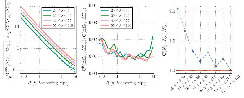
Figure 2 shows diagonal components of the covariance matrix estimated based on the above method. The left panel compares the full covariance with the shape noise contribution for the components involving the lensing profiles in four richness bins. The covariance diagonal amplitude, $\sqrt{{\bf C}(\Delta\Sigma_{\lambda_{\beta}},\Delta\Sigma_{\lambda_{\beta}})}$, decreases with radius as $1/R$ for the logarithmically-spacing bins up to $R\simeq 10~{}h^{-1}{\rm Mpc}$, reflecting the fact that the shape noise gives a dominant contribution in this radial scale. The sample variance starts to be non-negligible at the larger radii. The error amplitude is greater for the larger richness clusters because of the fewer clusters, thereby leading to the fewer lens-source pairs (therefore the larger shape noise contribution in relative). The maximum scale of $R=50~{}h^{-1}{\rm Mpc}$ is set by a size of the JK subregion. The middle panel displays the contribution of the random covariance for the covariance estimation of the lensing profile. We find that the effect of random subtraction is at a few percent level at most in the covariance amplitude and is not significant for the redMaPPer clusters (also see Shirasaki et al., 2017). The right panel shows diagonal components of the covariance involving the abundance ${\bf C}(N_{\lambda_{\alpha}},N_{\lambda_{\alpha}})$, compared to the Poisson term. The figure shows that the sample variance is significant for lower richness bins (Hu & Kravtsov, 2003; Takada & Bridle, 2007), while the Poisson contribution becomes dominate for a larger richness bin due to the fewer clusters.

Another important aspect of the covariance matrix is its off-diagonal components. It describes cross-correlations between observables at different bins. The correlated shape noise arising from a clustering of clusters causes such correlated errors in the lensing profiles at different bins (see equation 47 in Oguri & Takada, 2011). In addition, the sample variance causes such correlated scatters; for example, the same large-scale structure causes coherent scatters in the lensing profiles at different radial and/or richness bins as well as in the abundance (Takada & Bridle, 2007; Takada & Hu, 2013; Takada & Spergel, 2014). In particular, the cross-covariance between the abundance and the lensing profiles is caused by the super sample covariance.

The relative contribution of the off-diagonal components to the diagonal components can be quantified by the cross-correlation coefficient matrix, defined as

$$r_{ij}\equiv\frac{{\bf C}(D_{i},D_{j})}{\sqrt{{\bf C}(D_{i},D_{i}){\bf C}(D_{j},D_{j})}},$$ (28)

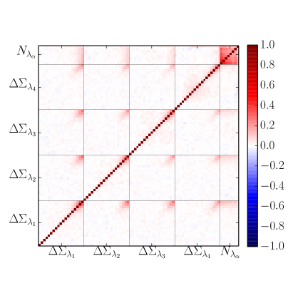
where $D_{i}$ is the $i$-th observables ($N_{\lambda_{\alpha}}$ or $\Delta\Sigma_{\lambda_{\beta}}$). Note $r_{ij}=1$ for $i=j$ by definition, and $r_{ij}\rightarrow 1$ means a strong correlation between data at the $i$- and $j$-th bins ($i\neq j$), while $r_{ij}=0$ denotes no correlation. Figure 3 shows the correlation coefficient matrix. There are non-vanishing cross-correlations between different bins of large radii $R\gtrsim 10~{}h^{-1}{\rm Mpc}$ for the lensing profiles and all the richness bins for the abundance. We will discuss the impact of the sample variance on the parameter estimation below.

5. Results

Figure 4.— Comparison of the best-fit model predictions with the lensing profile measurements in four richness bins (the left four panels) and the abundance measurements in eight richness bins (the right-lower panel), for the cluster sample of $20\leq\lambda\leq 100$. The orange shaded regions show the 16th and 84th percentiles of the model predictions computed from the MCMC chains, while the red points with error bars are the measurements. The errors are from the diagonal components of the covariance matrix. The black dashed curves in each panel are from the best-fit model with minimum $\chi^{2}$. The light-blue dashed curves in each panel of the lensing measurements are the best-fit models for the lensing profiles due to off-centered clusters in each richness bin (see around equation 27 for the modeling of the off-centering effects on the lensing profile). Note that the amplitudes of the off-centering lensing profile are not well constrained. At the upper right corner, we give the minimum value of reduced chi-square. We also give $\langle M_{\rm 200m}\rangle$ in each of the lensing plots and at the upper-right corner; the values are the median of the mean halo mass (weighted with the cosmological volume and the halo mass function) and its 16th and 84th percentiles that are computed from the MCMC chains of the mass-richness relation models.

Figure 5.— Similarly to the previous figure, but for the sample of $30\leq\lambda\leq 100$.

In this section, we show the main results of this paper; constraints on the mass-richness relation $P(\ln\lambda|M)$ from a joint fitting of the model to the abundance and lensing profiles, based on our forward modeling approach. In this analysis we do not vary cosmological parameters, and fix those to the Planck cosmology.

Figure 6.— The diagonal panels show the posterior distribution of each parameter of the mass-richness relation, and the other panels show the 68% and 95% CL contours of the MCMC chains in each two-parameter subspace. The red- and yellow-color results are for the samples of $20\leq\lambda\leq 100$ and $30\leq\lambda\leq 100$, respectively. The constraints include marginalization over other parameters including the off-centering parameters. Each parameter is well constrained compared to the flat priors in Table 2. A sharp bound of the contours in some parameters involving $\sigma_{0}$ or $q$, e.g. the lower-left corner of $(\sigma_{0},q$) subspace, is due to the condition $\sigma_{\ln\lambda|M}>0$ over the range of $10^{12}\leq M/[h^{-1}M_{\odot}]\leq 2\times 10^{15}$.

5.1. Parameter estimation

Once the halo emulator and the error covariance matrix are given as discussed in Section 4, we can constrain model parameters in the mass-richness relation, $P(\ln\lambda|M)$, by comparing the model predictions with the measurements of the abundance and the lensing profiles. We perform Bayesian parameter estimation assuming the Gaussian form, $\mathcal{L}\propto\exp(-\chi^{2}/2)$ , for the likelihood:

$$\chi^{2}=\sum_{i,j}~{}\Bigl{[}{\bf D}-{\bf D}^{\rm model}\Bigr{]}_{i}\left({\bf C}^{-1}\right)_{ij}\Bigl{[}{\bf D}-{\bf D}^{\rm model}\Bigr{]}_{j},$$ (29)

where ${\bf D}$ is the data vector that consists of the lensing profiles and the abundance in different radial and richness bins, ${\bf D}^{\rm model}$ is the model predictions, and ${\bf C}^{-1}$ is the inverse of the covariance matrix. Note that we use 19 radial bins in each richness bin, and that

$${\bf D}=\left\{\Delta\Sigma_{\lambda_{1}}(R_{1}),...\Delta\Sigma_{\lambda_{1}}(R_{19}),...\Delta\Sigma_{\lambda_{4}}(R_{19}),N_{\lambda_{1}},...N_{\lambda_{8}}\right\},$$

for the sample of $20\leq\lambda\leq 100$ and

$${\bf D}=\left\{\Delta\Sigma_{\lambda_{2}}(R_{1}),...\Delta\Sigma_{\lambda_{2}}(R_{19}),...\Delta\Sigma_{\lambda_{4}}(R_{19}),N_{\lambda_{3}},...N_{\lambda_{8}}\right\},$$

for the sample of $30\leq\lambda\leq 100$. The index $i$ and $j$ run over the different components of data, $i,j=1,2,\dots,84$ for the sample of $20\leq\lambda\leq 100$, while $i,j=1,2,\dots,63$ for the sample of $30\leq\lambda\leq 100$. We include nine model parameters for the former sample (four for the mass-richness relation and five for the off-centering effect as described in Section 3.3) or eight parameters for the latter sample, respectively. We use a Markov chain Monte Carlo (hereafter MCMC) method to perform an interference of the parameters. We use $\mathit{emcee}$ (Foreman-Mackey et al., 2013) for our parameter estimation. Table 2 summarizes the results of parameter estimation, which gives a description of each parameter, its prior, and the median and $68\%$ CL interval after removing the burn-in chains and marginalizing over other parameters. We use a flat prior for each parameter that has a sufficiently broad width as given in Table 2. The parameters of mass-richness relation $\{A,B,\sigma_{0},q\}$ are well constrained by the cluster observables, for both the samples of $20\leq\lambda\leq 100$ and $30\leq\lambda\leq 100$. The off-centering effects on the lensing profiles need to be included, but some of the off-centering parameters are not well constrained. This can be compared with the recent work in van Uitert et al. (2016), where the off-centering parameters are well constrained by jointly using the lensing profiles and the radial profiles of member galaxies.

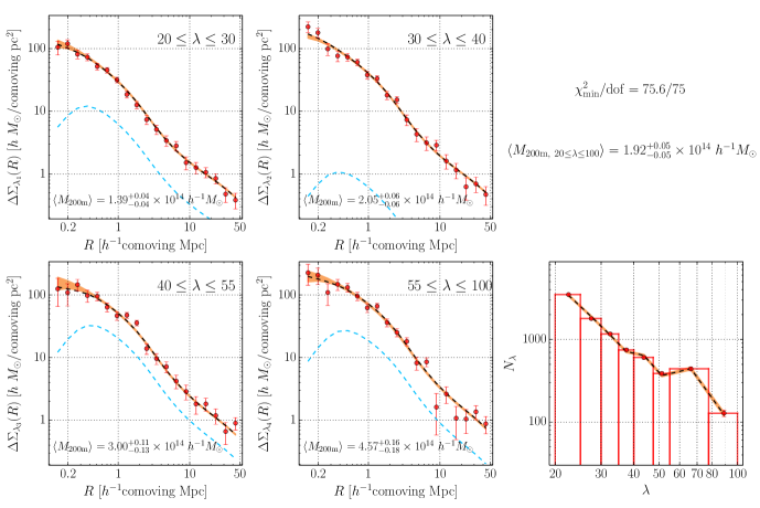
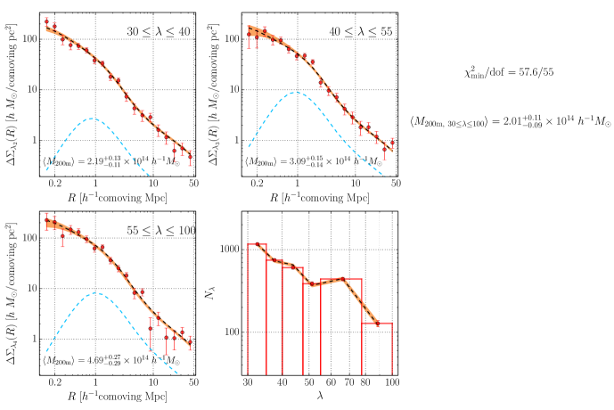
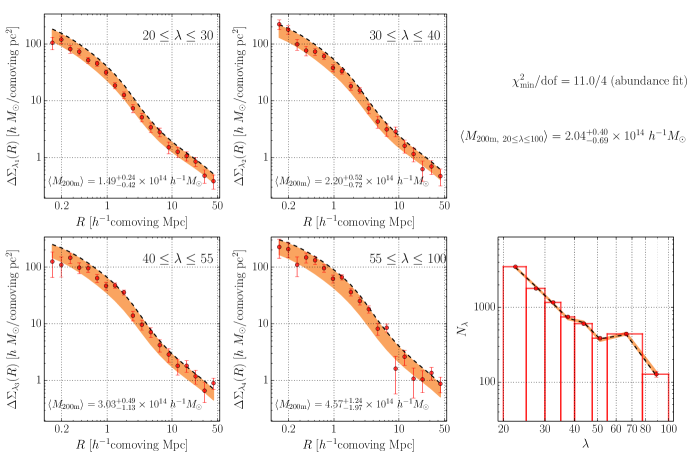
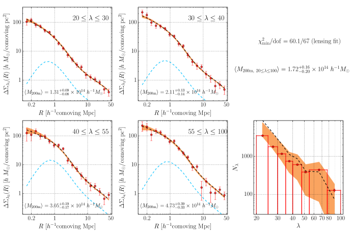
Figure 4 compares the best-fit model predictions with the measurements for both the lensing profiles in four richness bins and the abundance in eight richness bins, for the sample of $20\leq\lambda\leq 100$. The orange-color shaded regions in each panel denote the 68$\%$ CL intervals of the model predictions, obtained from the MCMC chains after marginalizing over the model parameters. The figure shows that our model remarkably well reproduces the lensing profiles and the abundance in the different richness bins simultaneously. The agreement implies the existence of a good model of the mass-richness relation that can reproduce the cluster observables for the Planck cosmology. The model mass-richness relation has sufficient flexibility to reproduce the observables by varying the model parameters. We would also like to stress that the model lensing profiles, computed from the $N$-body simulation based emulator, well reproduce the measurements in the different richness bins, including the 1-halo and 2-halo terms and the intermediate scales. The reduced chi-square for the best-fit model is $\chi^{2}_{\rm min}/{\rm dof}=75.6/75$ for 75 degrees of freedom $(75=84-9)$ with nine model parameters, meaning that the best-fit model gives a good fit. For reference, we show how a shift in each of the mass-richness relation parameters from the best-fit value, by an amount of the 68% CL interval in Table 2, changes the cluster observables in Appendix C, while fixing other parameters to their best-fit values. Figure 18 shows that the shift in each parameter changes the abundances and the lensing profiles in each richness bin in a complex way.

Similarly, even when we restrict ourselves to the subsample of clusters with larger richness $30\leq\lambda\leq 100$, our model can reproduce the measurements, as shown in Figure 5 and Table 2. The best-fit model is slightly different from that for the sample of $20\leq\lambda\leq 100$, but the two models agree with each other within their errors.

Figure 7.— The result of the analysis in the sample of $20\leq\lambda\leq 100$. Left: The joint probability distribution, $P(\ln M,\ln\lambda)$, from the best-fit model parameters for $P(\ln\lambda|M)$ using equation (30). We normalized the joint probability so as to satisfy the normalization condition $\int\!\mathrm{d}\ln\lambda\int\!\mathrm{d}\ln M~{}P(\ln M,\ln\lambda)=1$ for the range of $20\leq\lambda\leq 100$ and $10^{12}\leq M/[h^{-1}M_{\odot}]\leq 2\times 10^{15}$. For comparison, the solid red-color line shows the best-fit model for the mean mass-richness relation, $\langle\ln\lambda\rangle(M)$, given in equation (15) (see Table 3 for the parameter values), while the dashed lines show the 16th and 84th percentiles of $\ln\lambda$ distribution at a fixed mass (i.e. the width of $\sigma_{\ln\lambda|M}$ in equation 16). By projecting the joint probability distribution along halo mass in equation (32), we can compute the probability distribution of richness (i.e. the richness function) as shown in the right panel. It remarkably well reproduces the measurement denoted by the red points with error bars estimated from the Poisson noise at each of finer richness bins. On the other hand, the upper panel shows the probability distribution of halo mass for the redMaPPer clusters, computed by projecting the joint distribution along the richness in equation (33). The mean halo mass is found to be about $2\times 10^{14}h^{-1}M_{\odot}$ as shown in Figure 4. Right: Similarly to the left panel, but the probability distribution of halo mass for each of the four richness bins used in the lensing measurements. The solid curve in each color is the median, and the dashed lines denote the 16th and 84th percentiles computed from the MCMC chains.

Figure 8.— Similarly to the previous figure, but for the sample of $30\leq\lambda\leq 100$. The mass distribution at the lower mass is more suppressed compared to the result from the sample of $20\leq\lambda\leq 100$ in Figure 7.

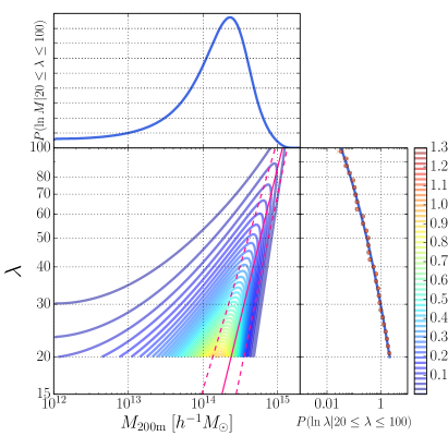
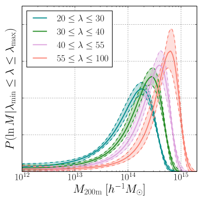
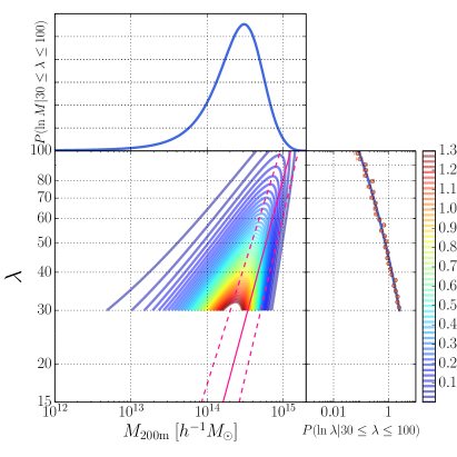
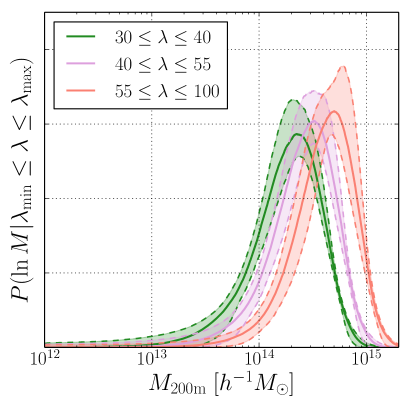
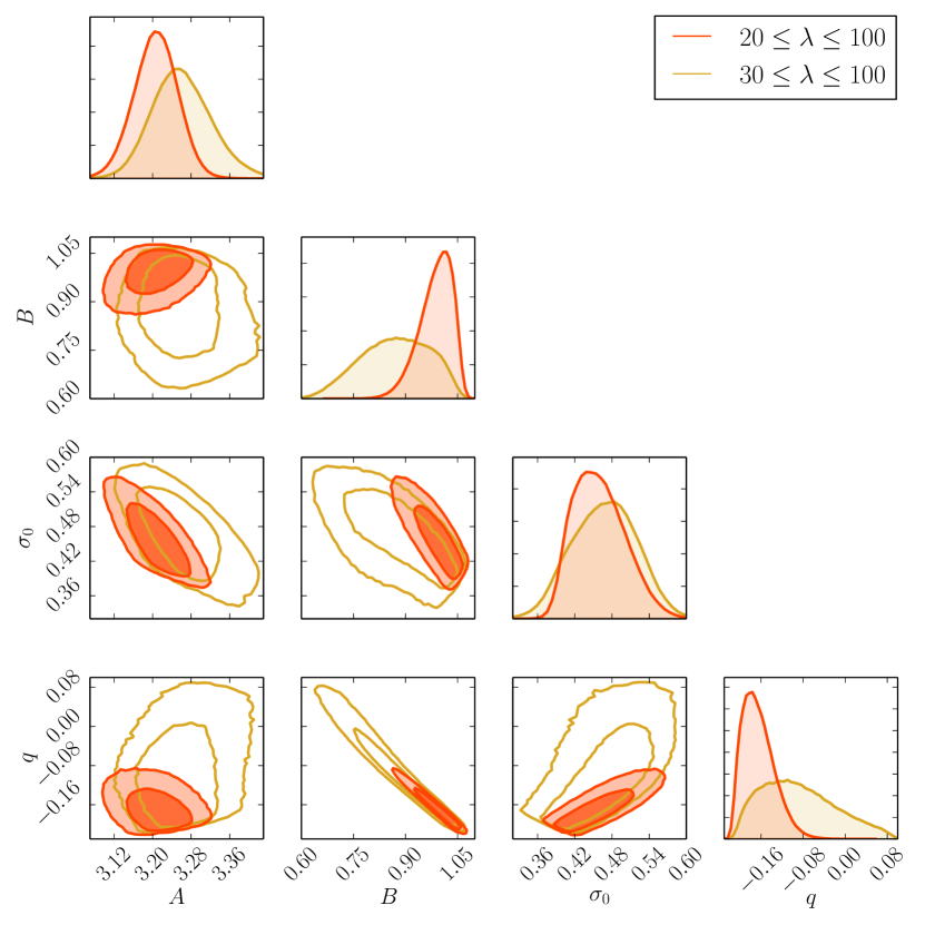
Figure 6 shows 68% and 95% CL contours for each pair of our four parameters used to model the mass-richness relation, after marginalizing over the off-centering parameters, while the one-dimensional histogram shows the posterior distribution of each parameter. Even though we employ a flat prior on each parameter, a joint measurement of the lensing profiles and the abundance allows us to well constrain each parameter. For the sample of $20\leq\lambda\leq 100$, a constant scatter in the mass-richness distribution, i.e. $q=0$, is strongly disfavored at about $5\sigma$. A negative value, $q=-0.169^{+0.035}_{-0.026}$ is favored, as given in Table 2, implying that the scatter starts to increase with decreasing halo mass. On the other hand, for the subsample of $30\leq\lambda\leq 100$, a constant scatter with $q=0$ is acceptable within the error bar. We will discuss the implication of these results below.

We can derive the joint probability distribution of $\lambda$ and $M$:

$$P(\ln M,\ln\lambda)\propto P(\ln\lambda|M)P(\ln M),$$ (30)

where $P(\ln M)$ is the probability distribution of halo mass. Note that the normalization factor is determined so as to satisfy the condition $\int\!\mathrm{d}\ln\lambda\int\!\mathrm{d}\ln M~{}P(\ln M,\ln\lambda)=1$ for the range of $\ln M$ and $\ln\lambda$, and we restrict the domain of $P(\ln M,\ln\lambda)$ to this range. For $P(\ln M)$, we employ the underlying mass function in the SDSS volume for the Planck cosmology:

$$P(\ln M)=\frac{\displaystyle\int_{z_{\rm min}}^{z_{\rm max}}\mathrm{d}z~{}\frac{\chi^{{{\color[rgb]{0,0,0}2}}}(z)}{H(z)}\frac{{\rm d}n(M,z)}{{\rm d}\ln M}}{\displaystyle\int_{\ln M_{\rm min}}^{\ln M_{\rm max}}\mathrm{d}\ln M\int_{z_{\rm min}}^{z_{\rm max}}\mathrm{d}z~{}\frac{\chi^{{{\color[rgb]{0,0,0}2}}}(z)}{H(z)}\frac{{\rm d}n(M,z)}{{\rm d}\ln M}}.~{}$$ (31)

For $P(\ln\lambda|M)$ in equation (30), we use the best-fit model in Table 2.

The contours in Figure 7 show the joint distribution $P(\ln M,\ln\lambda)$ in equation (30). For comparison, the red solid line shows the best-fit model for the mean of the mass-richness relation, $\langle\ln\lambda\rangle(M)$ (see equation 15), while the dashed lines show the 68% percentiles of the distribution of $\ln\lambda$ at a fixed halo mass (i.e. the width of $\sigma_{\ln\lambda|M}$ in equation 16). From equation (30), the joint probability has a power towards lower halo masses for each $\lambda$ bin due to the contribution of less massive halos via the halo mass function $P(\ln M)\propto\mathrm{d}n/\mathrm{d}\ln M$.

Integrating the joint probability $P(\ln M,\ln\lambda)$ along either the halo mass or the richness direction gives the distribution of $\ln\lambda$ or $\ln M$ for the sample of $20\leq\lambda\leq 100$:

$$P(\ln\lambda|\lambda_{\rm min}\leq\lambda\leq\lambda_{\rm max})=\int_{\ln M_{\rm min}}^{\ln M_{\rm max}}\mathrm{d}\ln M~{}P(\ln M,\ln\lambda)$$ (32)

or

$$P(\ln M|\lambda_{\rm min}\leq\lambda\leq\lambda_{\rm max})=\displaystyle\int_{\ln\lambda_{\rm min}}^{\ln\lambda_{\rm max}}\mathrm{d}\ln\lambda~{}P(\ln M,\ln\lambda).$$ (33)

The right panel in the left plot of Figure 7 gives the probability $P(\ln\lambda|20\leq\lambda\leq 100)$, showing that our model remarkably well reproduces the observed richness function at much finer bins than eight bins in Figure 4, over the entire range of richness. Similarly, the upper panel shows our model prediction for the probability of halo masses $P(\ln M|20\leq\lambda\leq 100)$ for the redMaPPer clusters. The probability implies that a typical halo mass of the redMaPPer clusters is about $M_{\rm 200m}=2\times 10^{14}h^{-1}M_{\odot}$. However, the distribution displays a long tail towards low mass, even down to $M=10^{12}h^{-1}M_{\odot}$ that is much smaller than a cluster mass scale. This might be an implication of residual systematic errors in our analysis or the redMaPPer catalog.

In addition, we can compute the expected mass distribution in each richness bin, $\lambda_{\alpha,\rm min}\leq\lambda\leq\lambda_{\alpha,\rm max}$, using equation (33) by replacing $\{\lambda_{\rm min},\lambda_{\rm max}\}$ with $\{\lambda_{\alpha,\rm min},\lambda_{\alpha,\rm max}\}$. The right plot of Figures 7 shows the result for the sample of $20\leq\lambda\leq 100$. The shaded region around each curve shows the 68% CL interval computed from the MCMC chains. Clearly, the lowest richness bin ($20\leq\lambda\leq 30$) favors the existence of low mass halos with $M\lesssim 10^{14}h^{-1}M_{\odot}$ and it requires about 10% contribution from even group- or galaxy-scale halos with $M\lesssim 10^{13}h^{-1}M_{\odot}$.

Figure 8 shows similar plots, but for the sample of $30\leq\lambda\leq 100$. Compared to Figure 7, this sample has a suppressed contribution of low mass halos with $M\lesssim 10^{13}h^{-1}M_{\odot}$.

5.2. Comparison of $P(\ln M|\lambda)$ with Simet et al.

Figure 9.— The conditional probability distribution $P(\ln M|\lambda)$ computed from the best-fit model parameters according to equation (36). The solid red or orange line denotes the median of the mass distribution at a fixed richness for the sample of $20\leq\lambda\leq 100$ or $30\leq\lambda\leq 100$, respectively. The dashed lines denote $\langle M|\lambda\rangle$ in the same colors. The respective shaded regions denote the range of the 16th and 84th percentiles of mass distribution at a fixed richness. Our results for the median and the mean relation agree especially at the high richness with the best-fit result in Simet et al. (2017) calculated from equation (34), denoted by the blue line, where $P(\ln M|\lambda)$ was estimated from the lensing information alone based on a backward modeling approach. However, our result shows the larger scatter than found in Simet et al. (2017) (see text for the discussion).

Figure 10.— Similarly to Figure 9, but a more quantitative comparison of our result with Simet et al. (2017) for the mass-richness relation, $P(\ln M|\lambda)$, for each of the samples of $20\leq\lambda\leq 100$ or $30\leq\lambda\leq 100$. Left: The red- and orange-color inner shaded regions show the 16th and 84th percentiles of the distribution of the mean halo mass $\langle M|\lambda\rangle$, computed from the MCMC chains for each cluster sample. The outer shaded region shows the 2nd and 98th percentiles and the middle line is the median of distribution. These results are shown relative to the S17 result, which is calculated from equations (34) and (35) as $\langle M|\lambda\rangle=\exp(\langle\ln M|\lambda\rangle+\sigma_{\ln M|\lambda}^{2}/2)$, with the best-fit parameters after equation (35). The blue shaded region around unity shows the same regions for the mean relation from the S17 result, inferred from the parameter constraints in S17 described after equation (35). Right: Similarly to the left panel, but this shows the results for the median relation. This shows only the 16th and 84th percentiles of the distribution. These results are also shown relative to the S17 result, which is calculated as $\exp(\langle\ln M|\lambda\rangle)$, with the best-fit parameters after equation (35).

Figure 11.— Similarly to Figure 9, but a more quantitative comparison of our result with Simet et al. (2017) for the mass-richness relation, $P(\ln M|\lambda)$, for each of the samples of $20\leq\lambda\leq 100$ or $30\leq\lambda\leq 100$. The red- and orange-color shaded regions show the 16th and 84th percentiles of the distribution of the scatters, $\sigma_{\ln M|\lambda}$, that characterize the width of halo mass distribution for a fixed richness (the half width of 68% CL region), computed from the MCMC chains for each sample (see text for details). The blue shaded region shows the S17 result from equation (35), where the error on $\sigma_{\ln M|\lambda}$ is estimated by propagating the uncertainties in the parameters in S17, which are described after equation (35). Note that the constraint of S17 on the scatter is mainly from the prior. The solid lines denote the median for the distributions.

We now compare our results with the recent results on redMaPPer clusters presented by Simet et al. (2017) (hereafter S17). S17 constrained the mass-richness relation of the SDSS redMaPPer clusters, $P(\ln M|\lambda)$, from the weak lensing measurements, using the backward modeling approach, and the abundance information was not included to constrain the mass-richness relation. In addition, S17 used an analytical model for the lensing profile, the Navarro-White-Frenk (NFW) model (Navarro et al., 1996), to compare with the measurements, although they instead used a narrow range of radii ($0.3\lesssim R\lesssim 3~{}h^{-1}{\rm Mpc}$), outside which the NFW profile ceases to be accurate, e.g. due to an imperfect treatment of the mass profile at the transition scales between the 1- and 2-halo terms (e.g., Diemer & Kravtsov, 2014). We should note that S17 adopted the flat $\Lambda{\rm CDM}$ model with $\Omega_{\rm m0}=0.30$ while we used the model with $\Omega_{\rm m0}=0.3156$. In the following comparison, we use a scaling in S17 (see their Section 6) to match their result to the model with $\Omega_{\rm m0}=0.3156$ for the definition of $M_{\rm 200m}$. This scaling decreases their normalization by 2.5%. We also note that the number of the clusters after similar richness and redshift cuts in S17 (5,570) is smaller than ours (8,312), mainly because S17 used a conservative shape catalog cut that removed all clusters in the Southern Galactic Cap. Here we briefly summarize the constraint in S17. In their model, the mean in $\log_{10}M$ for a fixed $\lambda$ is related to the mean in $\ln M$ as

$$\langle\log_{10}M|\lambda\rangle \equiv \int_{-\infty}^{+\infty}{\rm d}\ln M~{}P(\ln M|\lambda)\log_{10}M$$ (34)

$$= \log_{10}M_{0}+\alpha\log_{10}{\left(\frac{\lambda}{40}\right)}$$

$$= \frac{\langle\ln M|\lambda\rangle}{\ln{10}}.$$

Similarly, the scatter for a fixed $\lambda$ is expressed in terms of their parameters as

$$\sigma_{\ln M|\lambda}=\sqrt{\frac{\alpha^{2}}{\lambda}+\sigma_{\rm int}^{2}}.$$ (35)

In the following we used their best-fit parameters, $\{\log_{10}M_{0},\alpha,\sigma_{\rm int}\}$ are $\{14.344-0.706(\Omega_{\rm m0}-0.3),1.33,0.25\}$ for $\Omega_{\rm m0}=0.3156$. The standard deviations for $\log_{10}M_{0}$ and $\alpha$ are approximately $0.031$ (including the systematics after the quadrature sum) and $0.095$, respectively, and we checked that the distributions are approximated by Gaussian distributions with negligible correlation between $\log_{10}M_{0}$ and $\alpha$ based on the MCMC contour in S17. The constraint on $\sigma_{\rm int}$ was weak and largely determined by the flat prior of $[0.2,0.3]$. We will use these constraints (the Gaussian distributions for $\log_{10}M_{0}$ and $\alpha$ with the standard deviations, and the flat prior for $\sigma_{\rm int}$) in Figures 9, 10 and 11. Note that the median is calculated for the log-normal distribution as $\exp(\langle\ln M|\lambda\rangle)$ and the mean for $M$ at a fixed richness is $\langle M|\lambda\rangle=\exp(\langle\ln M|\lambda\rangle+\sigma_{\ln M|\lambda}^{2}/2)$.

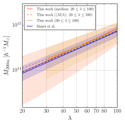
Based on our forward modeling results, we can compute the probability distribution $P(\ln M|\lambda)$ from $P(\ln\lambda|M)$ as

$$P(\ln M|\lambda)=\frac{P(\ln\lambda|M)P(\ln M)}{\displaystyle\int_{\ln M_{\rm min}}^{\ln M_{\rm max}}{\rm d}\ln M~{}P(\ln\lambda|M)P(\ln M)}.$$ (36)

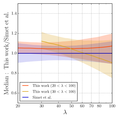
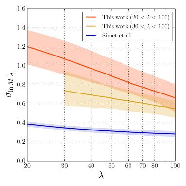
Figure 9 compares our result for $P(\ln M|\lambda)$ with that in S17 using the best-fit parameters. Note that $P(\ln M|\lambda)$ inferred from our model is not symmetric in the $\ln M$ space at a fixed richness, while $P(\ln M|\lambda)$ from S17 are symmetric because S17 assumed the log-normal probability for $P(\ln M|\lambda)$ instead of $P(\ln\lambda|M)$ as in our model. We also note that the mean $\langle M|\lambda\rangle$ is not the same as the median in both results. Here we show the median and the mean of the mass-richness relation for the comparison. Encouragingly the median and the mean relations, denoted by the solid or dashed lines, show a nice agreement with S17. This agreement probably reflects the fact that the average mass for a given richness bin is constrained by the measured amplitude of stacked cluster lensing profiles. The shaded region around each line denotes the 16th and 84th percentiles of $P(\ln M|\lambda)$ at a fixed richness. Our result indicates a much larger scatter than that in S17. As we will show below, the scatter is constrained by the joint abundance and lensing information. In other words, the scatter is very difficult to constrain with either of the two observables alone. The scatter we constrain with our model should include a total contribution of the richness measurement error, intrinsic scatter, orientation effects (Dietrich et al., 2014), and also possible projection effects (Eduardo Rozo for private communication). Rozo & Rykoff (2014) (also see Rozo et al., 2015a) studied the scatters for overlapping clusters between the redMaPPer clusters and the X-ray or Sunyaev-Zel’dovich clusters with high richness and low redshift, finding a smaller scatter $\sigma_{\ln M|\lambda}=0.25\pm 0.05$. However, the overlapping X-ray or SZ clusters are all massive (such as $10^{15}h^{-1}M_{\odot}$), and not necessarily representative of the SDSS redMaPPer clusters. S17 used this range for the flat prior of $\sigma_{\rm int}$ in equation (35), but the constraint on the scatter was largely determined from this prior rather than the data. In other words, the scatter is very difficult to constrain with the lensing information alone.

The orange-color shaded region in Figure 9 denotes the scatter obtained from the sample of $30\leq\lambda\leq 100$. The scatter for this sample is found to be somewhat smaller than that for the sample with $20\leq\lambda\leq 100$, implying that some contribution of the large scatter for the full sample is from low richness halos with $20\leq\lambda\leq 30$. We will discuss a possible origin of the apparently large scatters at lower richness bin in our results.

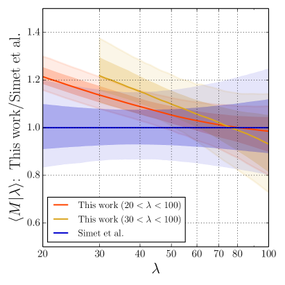
Figures 10 and 11 give a more quantitative comparison of our result with S17, for each of the samples of $20\leq\lambda\leq 100$ or $30\leq\lambda\leq 100$, respectively. The inner and outer shaded regions in the left panel of Figure 10 show the 2nd, 16th, 84th and 98th percentiles of the distribution of the mean for $\langle M|\lambda\rangle$ relation (not $\exp[\langle\ln M|\lambda\rangle]$), which are computed from the MCMC chains as a function of richness, and the middle solid curve is the median of the distribution. Similarly, the right panel of Figure 10 shows the 16th and 84th percentiles of the distribution of the median relation. Although the left panel of Figure 10 shows that our result is consistent with S17 within the confidence intervals, there is a mild disagreement in the mean relation, $\langle M|\lambda\rangle$, at low richness. Since the mean or median of the mass-richness relation is sensitive to the “shape” of $\ln M$ distribution in $P(\ln M|\lambda)$ at a fixed richness, the mild disagreement might be ascribed to the asymmetric distribution in our model, while the shape in S17 is symmetric as shown in Figure 9. Alternatively, this difference might be due to the assumed cosmological models in the parameter estimation where we employed the Planck cosmology in order to model the abundance and stacked lensing profiles. We also found that there is some disagreement in the lensing profiles around $R\sim 3\ h^{-1}{\rm Mpc}$ between the NFW profile and our simulation-calibrated emulator at a fixed halo mass. A further study would be needed to address the origin of the difference in more detail. Similarly, Figure 11 compares the scatter of the mass-richness relation, $\sigma_{\ln M|\lambda}$. Since our model generally predicts a skewed distribution of halo mass for a fixed richness value in $\ln M$ space, we compute the scatter as follows to compare with S17. First we compute the 16th and 84th percentiles of the mass distribution for a fixed richness as we did for the shaded region in Figure 9 from the MCMC chains. Then we assign the width as the half width of $68\%$ CL region in $\ln M$ space to the scatter $\sigma_{\ln M|\lambda}$; $\sigma_{\ln M|\lambda}\equiv(\ln M_{84}-\ln M_{16})/2$, where $M_{84}$ and $M_{16}$ are masses corresponding to the 84th and 16th percentiles, respectively. Then we compute the median and 68% interval of $\sigma_{\ln M|\lambda}$ from the MCMC chains, which are shown by the solid curve and the shaded region in Figure 11. The figure shows that our result implies a larger scatter than that implied in S17.

Finally we note that $P(\ln\lambda|M)$ is generally difficult to obtain if one uses the backward modeling method. In this case, $P(\ln\lambda|M)\propto P(\ln M|\lambda)P(\ln\lambda)$ needs to be computed and it requires a knowledge on the underlying distribution of richness parameters from the catalog for the halos with the smaller richness (i.e. including $\lambda\leq 20$ for the redMaPPer catalog). However, $P(\ln\lambda)$ is not generally available, or at least very noisy, for richness below a threshold richness ($\lambda=20$) in the current redMaPPer cluster catalog, because such low-richness clusters are by definition difficult to identify due to fewer member galaxies and masking effect, and would more suffer from systematic effects such as the projection effect.

6. Discussion

Our analysis we have so far shown involves some assumptions and uncertainties, and in this section we discuss the possible impacts on the results.

6.1. Information content and complementarity of abundance and stacked cluster lensing

Figure 12.— The posterior distribution of each parameter, and the 68% and 95% CL intervals in each two-parameter subspace for the MCMC chains when the mass-richness relation is constrained by the model fitting to the lensing (green) or abundance (blue) information alone. For comparison, the red contours show the results for the joint fitting in Figure 6. Here we used the sample of $20\leq\lambda\leq 100$. The posterior distribution becomes much wider due to strong degeneracies between the parameters. The star symbols in each color contours or the lines in the one-dimensional posterior distribution denote the best-fit model parameters. The best-fit model for the abundance alone is around the corner of the posterior distribution near the sharp bounds from the prior of $\sigma_{\ln\lambda|M}>0$ for the range of the halo mass in consideration.

Figure 13.— The left-side four panels show the model predictions for the lensing profiles computed from the MCMC chains, when the mass-richness relation is constrained by the abundance information alone, as shown by the blue contours in Figure 12. The right panel shows the fitting result for the abundance, and therefore shows that the model well reproduces the measurement. The orange-color shaded regions show the 16th and 84th percentiles computed from the MCMC chains. The black dashed curves in the left-side four panels from the best-fit model for abundance alone appear to be around edge of the intervals in the lensing profiles due to the skewed distribution (see Figure 19 for the detail) of the lensing predictions that are computed from the wide posterior distributions of the parameters in Figure 12. The lensing predictions from the best-fit model for abundance alone show systematically larger amplitudes than the measurement in each richness bin, especially for the lowest richness bin of $20\leq\lambda\leq 30$.

Figure 14.— As in Figure 13, but the right panel shows the model predictions of the abundances in each richness bin from the MCMC chains, when the mass-richness relation is constrained by the lensing information alone. The model inferred from the lensing measurements favors an inclusion of low richness clusters (see Figure 20 for the detail) at $20\leq\lambda\leq 30$, although the significance is not very high.

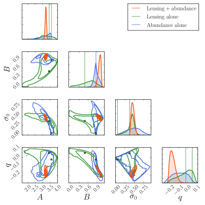
As we have shown, we can constrain the mass-richness relation from a joint fitting of the model predictions to the abundance and the lensing profiles. Firstly we study how the results are changed if using either alone of the two observables, or in other words how the joint fitting helps lift the parameter degeneracies. Figure 12 shows the 68% and 95% CL contours in the two parameter subspaces, as in Figure 6. The figure nicely shows that the two observables are complementary to each other, and the parameter degeneracies are efficiently broken when combining the two measurements. Either of the abundance or lensing information alone gives a wider distribution in each two-parameter subspace. It is also interesting to find that the parameter $B$ (the halo mass dependence of the mean mass-richness relation) or $\sigma_{0}$ (the normalization of the mass-richness scatter) is relatively better constrained by either one of the abundance or lensing information than another, respectively. The different sensitivities of the two observables to each parameter come from the different dependences on model parameters as shown in Figure 18.

We further study the complementarity of the two observables in Figures 13 and 14. Figure 13 shows the results if the mass-richness relation is constrained by the model fitting to the abundance alone. Our model well reproduces the abundance measurements in different richness bins, as shown by the lower right panel. The left-side four panels show the model predictions for the lensing profiles in each richness bin. The curve and the shaded regions in each panel for the lensing profile are not the fitting results, but rather the model predictions computed from the blue-color MCMC chains in Figure 12. Note that we did not include the off-centering parameters in the lensing model predictions, since there is no information in the abundance that can constrain the parameters, and we set $f_{\rm cen,\beta}=1$ to compute the model lensing profiles. The best-fit model for the abundance, denoted by the black dashed curve, predicts a systematically larger amplitude of the lensing profiles than the measurements over a range of the radial bins for each richness bin. In particular, the systematic offset is the largest for the lowest richness bin of $20\leq\lambda\leq 30$. This means that, if we naively reproduce the number of clusters at each richness bin by our model, the best-fit model favors a higher halo mass on average than the lensing measurements. As we discussed above, however, the abundance information alone suffers from severe degeneracies between the parameters. The shaded orange-color regions in each panel show the 68% CL intervals, which fairly well include the lensing measurements in each richness bin. This apparent agreement comes from the skewed distribution of the lensing profiles from the MCMC chains because the best-fit model is located at a corner in the broad posterior distributions of the parameters as shown in Figure 12. Hence, the best-fit model (blue line) appears to be located around the edge of the 68% CL interval of the lensing profiles in each richness bin. Figure 19 in Appendix D shows the posterior distribution of the lensing profile at some representative radial bins for each richness bin, which clearly shows a skewed distribution.

Similarly, Figure 14 shows the results if the mass-richness relation is constrained by the lensing information alone. In this case, we also included the off-centering parameters in the model fitting. Although our model perfectly reproduces the lensing profile measurements, the best-fit model predicts too many low-richness clusters at $\lambda\lesssim 30$. Even if we include the 68% CL intervals of model predictions inferred from the lensing data, shown by the orange color region, the models tend to predict somewhat larger abundances of low-richness clusters at $20\leq\lambda\lesssim 30$. This means that, since lower-richness clusters correspond to less massive halos, the measured lensing amplitudes favor to include a larger number of less massive halos in the low richness bins than the measured abundance. This result is consistent with Figure 13. Figure 20 in Appendix D shows the posterior distribution of the abundance in each richness bin.

Thus, summarizing the results in Figures 13 and 14, the best-fit models from the abundance and lensing measurements indicate a possible tension between the two observables, for the Planck cosmology. However, this does not appear to be very significant given the errors.

6.2. Halo mass information content in the 1- and 2-halo terms of lensing profiles

Figure 15.— The posterior distribution of each parameter as well as the 68% and 95% CL intervals in each two-parameter sub-space when using the lensing information at either of $R<10~{}h^{-1}{\rm Mpc}$ or $R>10~{}h^{-1}{\rm Mpc}$ alone, respectively, for the sample of $20\leq\lambda\leq 100$. Note that we did not use the abundance in these constraints, and the prior range is the same as in Table 2. For comparison, the green-color contours are the results from Figure 12 for the lensing alone using all the radial bins. The constraint from $R>10~{}h^{-1}{\rm Mpc}$ is so weak that the constraint mainly comes from the prior. The upper-left and lower-left boundaries of the contour in the $\sigma_{0}$-$q$ subspace are from the prior with the condition $\sigma_{\ln\lambda|M}>0$ for the range of halo masses we consider.

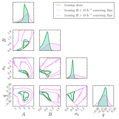
The weak gravitational lensing is a unique means of constraining the halo mass in the sample. The halo mass information is from the two regimes in the lensing profiles: the 1-halo term and the 2-halo term (Oguri & Takada, 2011), where the 2-halo term amplitude depends on halo mass via halo bias, because we have fixed the background cosmological model. Since the 1- and 2-halo terms have different dependences on halo mass, combining the two information might help improve constraints on the halo mass and therefore break the parameter degeneracies in the mass-richness relation. These halo mass dependences are properly included in the halo emulator we used for the model fitting. To study which of the 1- or 2-halo term information gives a dominant contribution to constrain the halo mass, we perform the model fitting only by using the lensing profile information at $R<10~{}h^{-1}{\rm Mpc}$ or $R>10~{}h^{-1}{\rm Mpc}$, which roughly corresponds to the transition between the 1- and 2-halo terms for the redMaPPer cluster-scale halos. Figure 15 shows the marginalized constraints on the parameters in the mass-richness relation, when using either alone of the lensing measurements. The constraint for the mass-richness relation comes dominantly from the lensing profiles at $R<10~{}h^{-1}{\rm Mpc}$. The constraint from $R>10~{}h^{-1}{\rm Mpc}$ comes mainly from the prior we used, and the mass information from the lensing at $R>10~{}h^{-1}{\rm Mpc}$ is very weak for the scales up to $50~{}h^{-1}{\rm Mpc}$. Future wide and deeper surveys might allow us to use more information in the 2-halo term, and helps improve the parameter constraints.

6.3. The impacts of possible systematic effects in the measurements

There might be residual systematic effects in the lensing and abundance measurements. In this subsection, we discuss the impact on the parameter estimation of the mass-richness relation.

An imperfect measurement of galaxy shapes or a systematic bias in photometric redshift estimates affects the lensing amplitudes we can measure via galaxy shapes. Following S17, we introduce an additional parameter, $m_{\rm lens}$, to model the possible residual systematic bias, and then study how this affects our estimation of the mass-richness relation parameters:

$$\widetilde{{\Delta\Sigma}_{\lambda_{\beta}}}(R;m_{\rm lens})=(1+m_{\rm lens}){\Delta\Sigma_{\lambda_{\beta}}}(R).$$ (37)

We assume a constant parameter $m_{\rm lens}$ for the lensing bias amplitudes in all the richness bins, and then allow $m_{\rm lens}$ to vary in the model fitting. We employ a flat prior of $-0.05\leq m_{\rm lens}\leq 0.05$. Table 4 shows that the parameters in the mass-richness relation are little changed, implying that the joint fitting is powerful to extract the parameters or allows for a self-calibration of the systematic errors (Oguri & Takada, 2011).

For the abundance measurement, an estimation of the effective survey area in equation (4) is somewhat tricky, as it requires to properly take into account the effects of survey masks and depth variations on cluster detection efficiency as a function of spatial positions in the survey footprint including the boundary regions. As can be found from Table 1, the correction for the effective survey area is largest for the clusters in the lowest richness bin, $20\leq\lambda\leq 25$, about 11% compared to the raw counts. We study the impact of a possible uncertainty in the effective area correction on the parameter estimation by enlarging the diagonal error bars of the abundance in each richness bin by an amount of the corrections in the counts in Table 1:

$${\bf C}(N_{\lambda_{\alpha}},N_{\lambda_{\alpha}})\rightarrow{\bf C}(N_{\lambda_{\alpha}},N_{\lambda_{\alpha}})+\left(N_{\lambda_{\alpha}}^{\rm corr}-N_{\lambda_{\alpha}}^{\rm raw}\right)^{2}.$$ (38)

As stated above, the second term amounts to about 11% fractional error in the counts for the lowest richness bin ($20\leq\lambda\leq 25$), compared to $1.7\%$ for the Poisson error (from $1/\sqrt{3488.4}$). Table 4 shows that each parameter is consistent with the result for the fiducial analysis in Table 3, to wihin the 68% CL interval.

In Table 4, we also study how the parameters are changed by including both the possible systematic effects in the lensing and abundance measurements. Again the parameters are not largely changed. Thus, the joint fitting seems robust against possible systematic effects because the two observables depend on the parameters in different ways.

Table 3 Variations in the parameters due to different analyses for the sample of $20\leq\lambda\leq 100$

Parameter	Crude covariance	Lensing alone	Abundance alone	1-halo lensing alone	2-halo lensing alone
				$R<10\ h^{-1}{\rm Mpc}$	$R>10\ h^{-1}{\rm Mpc}$
$A$	$3.215^{+0.036}_{-0.037}$ $(3.225)$	$3.191^{+0.415}_{-0.364}\ (3.425)$	$3.241^{+0.252}_{-0.482}\ (3.581)$	$3.194^{+0.420}_{-0.379}\ (3.410)$	$3.275^{+0.699}_{-1.077}\ (3.946)$
$B$	$0.994^{+0.037}_{-0.050}$ $(1.002)$	$0.636^{+0.208}_{-0.301}\ (0.491)$	$0.870^{+0.096}_{-0.066}\ (0.865)$	$0.638^{+0.208}_{-0.309}\ (0.446)$	$1.181^{+0.535}_{-0.543}\ (0.840)$
$\sigma_{0}$	$0.450^{+0.041}_{-0.035}$ $(0.440)$	$0.429^{+0.065}_{-0.114}\ (0.372)$	$0.483^{+0.186}_{-0.214}\ (0.043)$	$0.425^{+0.066}_{-0.117}\ (0.365)$	$0.723^{+0.434}_{-0.328}\ (0.017)$
$q$	$-0.170^{+0.031}_{-0.024}$ $(-0.175)$	$-0.020^{+0.066}_{-0.101}\ (0.048)$	$-0.087^{+0.083}_{-0.086}\ (-0.022)$	$-0.021^{+0.065}_{-0.103}\ (0.062)$	$-0.026^{+0.112}_{-0.148}\ (-0.001)$
$f_{\rm cen,1}$	$0.57^{+0.27}_{-0.36}$ $(0.78)$	$0.66^{+0.22}_{-0.38}\ (0.86)$	–	$0.66^{+0.22}_{-0.38}\ (0.90)$	$0.50^{+0.34}_{-0.34}\ (0.00)$
$f_{\rm cen,2}$	$0.81^{+0.14}_{-0.33}$ $(0.99)$	$0.81^{+0.13}_{-0.32}\ (0.89)$	–	$0.81^{+0.13}_{-0.31}\ (0.89)$	$0.50^{+0.34}_{-0.34}\ (0.70)$
$f_{\rm cen,3}$	$0.44^{+0.32}_{-0.30}$ $(0.70)$	$0.43^{+0.30}_{-0.29}\ (0.72)$	–	$0.43^{+0.30}_{-0.29}\ (0.69)$	$0.49^{+0.35}_{-0.34}\ (0.06)$
$f_{\rm cen,4}$	$0.57^{+0.27}_{-0.35}$ $(0.70)$	$0.58^{+0.26}_{-0.35}\ (0.80)$	–	$0.59^{+0.25}_{-0.35}\ (0.82)$	$0.50^{+0.34}_{-0.34}\ (0.35)$
$\alpha_{\rm off}$	$0.065^{+0.052}_{-0.030}$ $(0.152)$	$0.073^{+0.071}_{-0.034}\ (0.266)$	–	$0.074^{+0.076}_{-0.034}\ (0.304)$	$0.495^{+0.342}_{-0.334}\ (0.218)$

Note. — The first column, labeled by “Crude covariance”, shows the results for parameter estimation when using the covariance that includes only the shape noise contribution for the lensing profiles and the Poisson contribution for the abundances as described in Section 4.2. The second and third columns show the results when using either alone of the lensing or abundance information, respectively. Furthermore, the fourth and fifth columns show the results when using the lensing information at $R<10~{}h^{-1}{\rm Mpc}$ or $R>10~{}h^{-1}{\rm Mpc}$ alone, corresponding to the 1- and 2-halo term information, in the analysis of the lensing information alone. The priors for the parameters are the same as in Table 2.

Table 4 The impacts of possible residual systematic errors on the parameters for the sample of $20\leq\lambda\leq 100$

Parameter	+lensing sys.	+abundance sys.	+lensing and abundance sys.
$A$	$3.212^{+0.054}_{-0.057}\ (3.241)$	$3.207^{+0.043}_{-0.044}\ (3.236)$	$3.210^{+0.055}_{-0.054}\ (3.201)$
$B$	$0.991^{+0.042}_{-0.056}\ (0.988)$	$1.017^{+0.038}_{-0.054}\ (1.030)$	$1.014^{+0.039}_{-0.055}\ (1.044)$
$\sigma_{0}$	$0.453^{+0.048}_{-0.039}\ (0.442)$	$0.452^{+0.044}_{-0.034}\ (0.437)$	$0.450^{+0.045}_{-0.036}\ (0.441)$
$q$	$-0.168^{+0.036}_{-0.027}\ (-0.165)$	$-0.179^{+0.032}_{-0.023}\ (-0.184)$	$-0.177^{+0.034}_{-0.024}\ (-0.197)$
$f_{\rm cen,1}$	$0.57^{+0.27}_{-0.36}\ (0.80)$	$0.57^{+0.27}_{-0.36}\ (0.78)$	$0.57^{+0.27}_{-0.36}\ (0.82)$
$f_{\rm cen,2}$	$0.81^{+0.14}_{-0.35}\ (0.97)$	$0.81^{+0.14}_{-0.35}\ (1.00)$	$0.81^{+0.14}_{-0.35}\ (0.98)$
$f_{\rm cen,3}$	$0.43^{+0.32}_{-0.30}\ (0.55)$	$0.44^{+0.32}_{-0.30}\ (0.53)$	$0.45^{+0.32}_{-0.31}\ (0.61)$
$f_{\rm cen,4}$	$0.57^{+0.27}_{-0.34}\ (0.63)$	$0.57^{+0.27}_{-0.35}\ (0.62)$	$0.57^{+0.28}_{-0.35}\ (0.69)$
$\alpha_{\rm off}$	$0.064^{+0.049}_{-0.031}\ (0.117)$	$0.062^{+0.047}_{-0.031}\ (0.113)$	$0.062^{+0.051}_{-0.031}\ (0.151)$
$m_{\rm lens}$	$-0.005^{+0.036}_{-0.031}\ (-0.013)$	–	$-0.002^{+0.035}_{-0.033}\ (0.032)$

Note. — The second column shows how the parameters are changed by introducing additional parameter $m_{\rm lens}$ to model a possible residual, multiplicative error in the galaxy shape measurements. We employ the flat prior for $m_{\rm lens}$ as $(-0.05,0.05)$. The priors for other parameters are the same as in Table 2. The third column shows the results when enlarging the errors of the abundance measurements in each richness bin by an amount of the effective area correction according to equation (38). The fourth column shows the results when including the two effects.

6.4. The impact of the non-Gaussian sample variance

An accurate estimation of the non-Gaussian sample variance is one of challenging issues for ongoing and upcoming surveys. In this paper we used the 108 SDSS mock catalogs to estimate the error covariance matrix as described in Section 4.2. By using the full-sky simulations, the covariance we estimated includes the super-sample covariance contribution that arises from large-scale density fluctuations over the SDSS footprint, which is difficult to accurately estimate without the full-sky simulations. In Table 2, we show how the parameter estimation is changed when we use the crude covariance as described in Section 4.2 that includes only the shape noise contribution for the weak lensing measurements and the Poisson noise for the abundance. The median and best-fit values of the model are almost unchanged compared to the fiducial result in Table 3, implying that the shape noise and Poisson noise give a dominant contribution to the covariance. The 68% CL interval for each parameter from the fiducial analysis is only slightly enlarged, by up to about 15% for some parameter compared to the analysis using the crude covariance. Thus, we conclude that, for the SDSS data which is a relatively shallow survey, the impact of the non-Gaussian sample variance is not significant.

6.5. Projection effect in the SDSS redMaPPer catalog

Table 5Parameter estimation for the more flexible model of mass-richness relation (equation 39) for the sample of $20\leq\lambda\leq 100$

Parameter	Prior	Median and error
$A$	$(0.5,5.0)$	$3.236^{+0.071}_{-0.075}\ (3.334)$
$B$	$(-2.0,2.0)$	$0.996^{+0.047}_{-0.058}\ (1.066)$
$C$	$(-1.5,1.5)$	$0.001^{+0.035}_{-0.030}\ (-0.004)$
$\sigma_{0}$	$(0.0,1.5)$	$0.441^{+0.065}_{-0.088}\ (0.320)$
$q$	$(-2.0,2.0)$	$-0.158^{+0.046}_{-0.030}\ (-0.187)$
$p$	$(-2.0,2.0)$	$0.006^{+0.017}_{-0.023}\ (0.011)$
$f_{\rm cen,1}$	$(0.0,1.0)$	$0.56^{+0.27}_{-0.35}\ (0.81)$
$f_{\rm cen,2}$	$(0.0,1.0)$	$0.80^{+0.14}_{-0.34}\ (0.97)$
$f_{\rm cen,3}$	$(0.0,1.0)$	$0.43^{+0.32}_{-0.30}\ (0.56)$
$f_{\rm cen,4}$	$(0.0,1.0)$	$0.58^{+0.28}_{-0.35}\ (0.70)$
$\alpha_{\rm off}$	$(10^{-4},1.0)$	$0.062^{+0.049}_{-0.031}\ (0.134)$

Note. — We increased the range of priors for $B$ and $q$ from Table 2 to be more flexible with $C$ and $p$. In addition, we impose the condition $\sigma_{\ln\lambda|M}>0$ over the range of halo masses we consider; $10^{12}\leq M/[h^{-1}M_{\odot}]\leq 2\times 10^{15}$.

Our fitting result in Figure 7 indicates that very low mass halos ($M\lesssim 10^{13}\ h^{-1}M_{\odot}$) contribute to the sample in the lowest richness bin ($20\leq\lambda\leq 30$) by about 10% fraction. As one of the possibilities, this result may indicate the projection effects in the SDSS redMaPPer clusters; i.e. multiple halos along the line-of-sight direction are misidentified as one cluster after projection (Cohn et al., 2007).

As we showed in Figures 9 and 11, our model favors a large scatter in mass at a fixed richness. There are signatures on the existence of such low mass halos from both the lensing and abundance information as described in Section 6.1. If we naively reproduce the abundance of low richness halos just by the mass-richness relation in our model, the model predicts greater amplitudes of the lensing profiles than the measurements (Figure 13). Similarly, if we naively reproduce the lensing amplitudes in the low richness bin, the model predicts somewhat large abundance of low-richness clusters that correspond to less massive halos. To reconcile these discrepancies with our model within the Planck cosmology, we need to introduce a relatively large scatter in the mass-richness relation, which yields an inclusion of such low mass halos into the sample, especially for the sample of $20\leq\lambda\leq 100$. To arrive at these results, we assume a single population of the underlying clusters and the distribution of richness parameters at a fixed halo mass obeys a log-normal distribution. In some sense the scatter amplitude we found could be understood as the total contribution that includes the intrinsic scatter, the richness estimation errors, and a possible contamination of the projection effect. To study the impact of the projection effects, we need mock catalogs that are carefully designed and built in redshift space, using light-cone simulations, in order to estimate how the projection effects affect the redMaPPer cluster finder as well as the lensing and abundance measurements. This is beyond the scope of this paper, and we will study this elsewhere (see below for further discussion).

Figure 16.— Similarly to the right panel of Figure 7, but from the more flexible model. This more flexible model also favors too low mass contribution ($M_{\rm 200m}\lesssim 10^{13}h^{-1}M_{\odot}$) as in the result of the fiducial model in Figure 7.

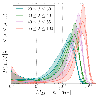
Instead we here study how a more flexible model of the mass-richness relation changes our results within the log-normal model for $P(\ln\lambda|M)$. To study this, we introduce more free parameters to model the mean of the mass-richness relation as well as the scatters from equations (15) and (16):

$$\langle\ln\lambda\rangle(M)=A+B\ln\left(\frac{M}{M_{\rm pivot}}\right)+C\left[\ln\left(\frac{M}{M_{\rm pivot}}\right)\right]^{2},$$

$$\sigma_{\ln\lambda|M}=\sigma_{0}+q\ln\left(\frac{M}{M_{\rm pivot}}\right)+p\left[\ln\left(\frac{M}{M_{\rm pivot}}\right)\right]^{2},$$ (39)

The parameters $C$ and $p$ model nonlinear halo mass dependences in the $\ln\lambda$-$\ln M$ space for the mean relation and the scatter, respectively. Table 5 summarizes the results of parameter estimation, showing that each parameter is consistent with the result in Table 2 for the fiducial analysis to within its 68% CL interval. The parameters $C$ and $p$ are consistent with zero to within the error bars, and thus we do not find a strong evidence on the nonlinear mass dependence in the mean mass-richness relation and its scatter. The minimum chi-square value of the more flexible model is $\chi^{2}_{\rm min}=75.2$, which differs from that of the fiducial analysis only by $\Delta\chi^{2}_{\rm min}=0.4$ ($\chi^{2}_{\rm min}=75.6$ for the fiducial model), suggesting that our fiducial model has a sufficient flexibility to model the mass-richness relation for the redMaPPer clusters, for the Planck cosmology. Figure 16 shows the distribution of halo masses for each richness bin, obtained from the MCMC chains for the more flexible model. Even this model favors an inclusion of low mass halos ($M\lesssim 10^{13}h^{-1}M_{\odot}$) into the sample via a convolution of the mass-richness relation with the halo mass function similarly to what we found in Figure 7.

7. Conclusion

In this paper, we have developed a method to constrain the mass-richness relation from the joint fitting to the abundance and the lensing profiles in different richness bins using the forward modeling approach, where we model the probability distribution of $\lambda$ at a given mass $M$, $P(\ln\lambda|M)$. In contrast the backward approach models the probability distribution of mass at a given richness, $P(\ln M|\lambda)$, which is often employed in the previous works (e.g., Baxter et al., 2016; Simet et al., 2017; Melchior et al., 2017). The forward method allows for a more direct comparison of the model prediction with the measurements.

To accurately model the cluster observables, we have used the halo emulator to interpolate the halo mass function and the stacked lensing profile as a function of halo mass and redshift for the Planck cosmology. We developed a pipeline that allows a sufficiently fast computation of the cluster observables based on the emulator in order to perform parameter estimation using the MCMC technique. We applied this method to the SDSS redMaPPer clusters, and constrained the mass-richness relation for the Planck cosmology.

We showed that, if we employ the log-normal distribution model for $P(\ln\lambda|M)$, our model can well reproduce both the abundance and the lensing profiles in different richness bins simultaneously for the Planck cosmology (see Table 2 and Figure 6). We found that, in these constraints, the lensing and abundance information are complementary to each other, and the combination efficiently lifts the parameter degeneracies as shown in Figure 12. Our method allows us to estimate the probability in the backward method, $P(\ln M|\lambda)$, by transforming the best-fit model of $P(\ln\lambda|M)$ weighted with the halo mass function, based on the Bayes theorem (equation 36). We showed that our result is consistent with that of the median and the mean relation in Simet et al. (2017) (see Figures 9 and 10), which was estimated based on the backward method using the lensing information alone.

However, the models preferred in our method predict a contribution of less massive halos to the sample. When we use the cluster sample with richness $20\leq\lambda\leq 100$, the best-fit model requires a non-negligible contribution ($\simeq 10\%$) of halos with $M\lesssim 10^{13}\ h^{-1}M_{\odot}$ to the sample (see Figure 7). We also showed that the best-fit parameters from either of the abundance or the lensing profiles alone are slightly inconsistent with each other (see Figures 13 and 14). The contributions of too low mass halos are unphysical since such halos cannot be recognized as massive clusters of galaxies. The unphysical contribution might be due to the fact that the Planck cosmology we have assumed throughout this paper is different from the underlying true cosmology of the universe. This would be interesting to further explore. However, we think that a more likely origin is due to residual systematic effects in the redMaPPer cluster catalog as indicated by the recent several works (Zu et al., 2017; Busch & White, 2017) (also see Sunayama, More et al. in preparation). Hence we need to further study the nature of the SDSS redMaPPer clusters.

Our analysis involves several assumptions. The most critical one is that we assumed that the redMaPPer clusters obey statistical isotropy. More exactly, to compute the cluster observables, we first compute the three-dimensional mass function and the halo-matter cross-correlation functions from $N$-body simulation outputs and then constructed the model predictions of the cluster observables, the abundance and the lensing profiles, by projecting the three-dimensional model ingredients along the line-of-sight direction. These procedures are violated if the redMaPPer clusters are affected by the projection effects, such as a mis-identification of different halos (clusters) along the line-of-sight direction as one halo (cluster). The amount of the projection effect would depend on the orientation of a halo shape and/or the surrounding large-scale structure with respect to the line-of-sight direction. In addition the projection effects would be more significant for low-richness clusters, because low mass halos have a higher chance of the projection effect due to their larger abundances, and have the larger measurement errors in the richness estimation due to fewer member galaxies. The larger scatters at low mass bins we found in this work might be a signature of the projection effects.

In order to properly address the projection effects, we need to use the mock catalogs of the SDSS redMaPPer clusters in the light cone simulation. For this purpose, the forward method we developed in this work would be very useful. Firstly, with the initial guess of the mass-richness relation $P(\ln\lambda|M)$, we can populate hypothetical members galaxies into each halo from their mass $M$ in a light-cone realization. This richness assignment to halos in the simulation is difficult for the backward method if using $P(\ln M|\lambda)$. Secondly, we project the mock clusters along the line-of-sight direction to re-define a “hypothetically-observed” richness of each cluster on the sky, based on the SDSS redMaPPer algorithm (circular aperture and redshift width), where multiple halos can be merged into one detection to have the summed richness parameter if the halos are aligned along the line-of-sight direction within a circular aperture ($\simeq 1\ h^{-1}{\rm Mpc}$ radius) in equation (2) on the sky. Then, we can make the hypothetical measurements of the lensing profiles and the abundances from the mock catalogs of the SDSS redMaPPer clusters in the simulations. If the obtained lensing profiles and the abundances show a deviation from the actual measurements, we can perturb the input mass-richness relation, and perform the above procedures again. Such an iterative method enables us to estimate a more accurate model for the mass-richness relation mitigating the projection effects. We believe that this is doable with the forward method, and this is our future work.

Our method further assumes that the cluster observables depend only on halo mass, and the redMaPPer clusters are a representative sample of the underlying halos in terms of their respective masses. Properties of clusters might also depend on a secondary parameter besides mass, such as the assembly history of each cluster – the so-called assembly bias (Miyatake et al., 2016; More et al., 2016). If the redMaPPer clusters are affected by the assembly bias, the constraints on the mass-richness relation would be biased, even if there is no projection effect. This would complicate the method in both theory and observation sides. On theory side, we need to properly take into account such an assembly bias effect in the model prediction. On observation side, a secondary parameter besides richness needs to be inferred for each cluster, in order to track the possible effect in individual cluster basis. For example, the concentration parameter, if estimated from the data itself, can be a good proxy of the assembly bias effect. However, such a secondary parameter is difficult to estimate, or at least it causes an additional scatter in relating the observables to the properties of the underlying halos. This also needs to be studied carefully.

The method and results shown in this paper are the first step towards the use of optical cluster for attaining high-precision cluster based cosmological information. Luckily, there are various kinds of cluster observables: X-ray, the SZ effect, the auto-correlation function, the redshift-space distortions (Okumura et al., 2017), and the cross-correlation with other populations of galaxies. There is a strong hope that we can combine these observables to disentangle cosmological information from systematic/astrophysical effects. The forward modeling approach used in this paper would be useful for such a study.

8. Acknowledgment

We thank Rachel Mandelbaum for making the shape catalog available to us. We thank Nick Battaglia, Eric Baxter, Matteo Costanzi, Masamune Oguri, Eduardo Rozo, Eli Rykoff, Emmanuel Schaan and Melanie Simet for useful discussion. We also thank the anonymous referee for helpful comments that improved the quality of this work. RM and KO acknowledge supports from Advanced Leading Graduate Course for Photon Science, and RM, MS and KO acknowledge supports from Research Fellowships of the Japan Society for the Promotion of Science for Young Scientists. RM also acknowledges a financial support from the University of Tokyo-Princeton strategic partnership grant, and greatly thanks Prof. David Spergel and members at the cosmology group of the Princeton University for their warm hospitality during his stay, where this work was initiated. This work was in part supported by Grant-in-Aid for Scientific Research from the JSPS Promotion of Science (No. 23340061, 26610058, 15H03654, 16H01089, 17J00658, 16J01512, 17K14273, and 17H01131), MEXT Grant-in-Aid for Scientific Research on Innovative Areas (No. 15H05887, 15H05893, 15K21733, and 15H05892) and by JSPS Program for Advancing Strategic International Networks to Accelerate the Circulation of Talented Researchers. TN acknowledges financial support from JST CREST Grant Number JPMJCR1414. HM is supported by the Jet Propulsion Laboratory, California Institute of Technology, under a contract with the National Aeronautics and Space Administration. Numerical computations presented in this paper were in part carried out on the general-purpose PC farm and Cray XC30 at Center for Computational Astrophysics, CfCA, of National Astronomical Observatory of Japan.

Appendix A Boost factor

Here we show the boost factor that is used to correct for a possible contamination of member galaxies in the source catalog for the stacked cluster lensing measurements (equation 12). Figure 17 shows the radial profile of the estimated boost factor for each richness bin. The boost factor correction is significant at radii $R\lesssim 1~{}h^{-1}{\rm Mpc}$ for all richness bins, and becomes small at the larger radii.

Figure 17.— The measurement of the boost factor according to equation (12).

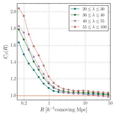
Appendix B Covariance estimation

Motivated by the theory for the covariance matrix of cluster abundance and stacked lensing (Hu & Kravtsov, 2003; Takada & Bridle, 2007; Oguri & Takada, 2011; Takada & Hu, 2013; Shirasaki et al., 2017; Singh et al., 2017), we use the 108 realizations of SDSS mock catalogs to estimate the covariance matrix for the lensing profiles and the abundance by breaking down the matrix into different contributions:

$${\bf C}(D_{i},D_{j}) \equiv \langle D_{i}D_{j}\rangle-\langle D_{i}\rangle\langle D_{j}\rangle$$ (B1)

$$= {\bf C}^{\rm SN}+{\bf C}^{\rm SV}-{\bf C}^{\rm R},$$

where ${\bf C}$ is the full covariance, ${\bf C}^{\rm SN}$ is the covariance matrix arising from the shape noise contribution, ${\bf C}^{\rm SV}$ is the sample variance contribution, and ${\bf C}^{\rm R}$ is the term corresponding to the random catalog subtraction in Section 2.3 of Singh et al. (2017). Here, ${\bf D}$ is the data vector that consists of the lensing profiles and the abundance in different radial and richness bins (see Table 1):

$${\bf D}\equiv\left\{\Delta\Sigma_{\lambda_{1}}(R_{1}),...\Delta\Sigma_{\lambda_{1}}(R_{19}),...\Delta\Sigma_{\lambda_{4}}(R_{19}),N_{\lambda_{1}},...N_{\lambda_{8}}\right\},$$ (B2)

and $D_{i}$ denotes $i$-th component. The dimension of the data vector is 84 for the cluster sample of $20\leq\lambda\leq 100$, while 63 for the sample of $30\leq\lambda\leq 100$, because we use 19 radial bins in each of four or three richness bins for the lensing profiles, and eight or six richness bins for the abundance. In the following, we describe how we estimate each term in equation (B1).

B.1. Shape noise contribution: ${\bf C}^{\rm SN}$

The intrinsic shape causes statistical uncertainties in the stacked cluster lensing measurement, due to a finite number of source-cluster (lens) pairs used in the analysis. For the relatively shallow SDSS data, where a typical number density of source galaxies is about $1~{}$arcmin^-2, the shape noise gives a dominant source of the covariance matrix components involving $\Delta\Sigma_{\lambda_{\beta}}$. To estimate the shape noise contribution, we use the real catalog of source galaxies as well as the redMaPPer clusters, because the real catalog includes various observational effects such as spatial variations of data quality and masks. We estimate the shape noise contribution as follows. Firstly, we randomly rotate the ellipticity orientation of each galaxy, in order to erase the real lensing signal. Then we measure the stacked lensing profile for the redMaPPer clusters, in each richness bin, in the exactly same manner as we did in the actual measurement, including the corrections of boost factor and photo-$z$ errors in Section 2.3. Note that we used the Planck cosmology in this estimation and therefore use the exactly same number of pairs of source galaxies and redMaPPer clusters as in the actual measurement. Using 10,000 realizations of the lensing profile measurements after random rotations, we estimate the shape noise contribution to the covariance matrix as

$${\bf C}^{\rm SN}(D_{i},D_{j})=\frac{1}{N_{\rm SN}-1}\sum_{a=1}^{N_{\rm SN}}[D^{\rm SN}_{a,i}-\overline{D}{}^{\rm SN}_{i}][{D}^{\rm SN}_{a,j}-\overline{D}{}^{\rm SN}_{j}],$$ (B3)

where $N_{\rm SN}=10,000$, quantities with superscript “SN” denote the measurements from the realization after random rotation of individual galaxy ellipticities, $D^{\rm SN}_{a,i}$ is the lensing measurement at the $i$-th lensing bin from the $a$-th realization, i.e. $D^{\rm SN}_{a,i}\equiv\widehat{\Delta\Sigma}_{(a)\lambda_{\beta}}(R_{j})$, and $\overline{D}{}^{\rm SN}_{i}$ is the average, defined as $\overline{D}{}^{\rm SN}_{i}\equiv(1/N_{\rm SN})\sum_{a}D^{\rm SN}_{a,i}$. The estimate of the shape noise covariance is clean since the expected noise in its inverse is at the level of 1% based on Hartlap et al. (2007) from $N_{\rm SN}=10,000$ and the total number of richness and radial bins (76 for the sample of $20<\lambda<100$). The cross-covariance between the abundance and the shape noise term is vanishing because of no correlation between the shape noise and the abundance (Takada & Bridle, 2007; Oguri & Takada, 2011). Hence we ignore the cross-covariance between shape noise and abundance.

B.2. Sample variance: ${\bf C}^{\rm SV}$

The sample variance arises due to an imperfect sampling of the fluctuations in large-scale structure from a finite survey volume. This contribution itself depends on the statistical nature of large-scale structure, and therefore on cosmology. To estimate the sample variance effects on the cluster observables, we use the 108 realizations of the SDSS mock catalogs as follows. Firstly, we insert each source galaxy into the light-cone simulation according to the angular positions and best-fit photo-$z$, and then simulate lensing distortion effect on the galaxy due to foreground structures. Here we ignore intrinsic shapes when creating the mock catalogs. Secondly, we use the halos with assigned hypothetical richness to calculate the covariance for abundance and lensing profile in each realization as below.

There are various contributions to the sample variance; the Gaussian contribution arising from products of two-point correlation functions of lensing fields and cluster distribution, and the non-Gaussian contribution arising from the four-point functions of matter and cluster fields at the lens redshift (Takada & Bridle, 2007; Takada & Hu, 2013; Gruen et al., 2015; Shirasaki et al., 2017). It is still difficult to study these different contributions separately (Takahashi, Takada et al. in prep.).

In this paper, we use the jackknife method (JK) to estimate the sample variance. The JK method is one of the statistical techniques (Efron, 1982), which has also been applied to an estimation of the covariance matrix for the galaxy (cluster)-galaxy weak lensing measurements (e.g. Mandelbaum et al., 2013; Coupon et al., 2015; Miyatake et al., 2016; Clampitt et al., 2017). As carefully shown in Shirasaki et al. (2017), the JK method gives a fairly accurate estimation of the underlying covariance matrix.

We combine the 108 realizations to estimate the sample variance contribution to the covariance matrix based on the JK method, as follows. Firstly, we estimate the covariance matrix from the $\alpha$-th realization; (1) Divide the hypothetical SDSS survey region into different $N_{\rm sub}$ subregions, where the area of each subregion is roughly equal. (2) Measure the abundance and the stacked lensing profiles for mock SDSS redMaPPer clusters in each richness bin, from the survey region excluding the $\beta$-th JK subregion. (3) Repeat the (2) measurement for all the $N_{\rm sub}$ subsamples and build the $N_{\rm sub}$ JK resamples of the measurements. Then we estimate the covariance for the $\alpha$-th realization as

$${\bf\bf C}^{\rm JK}_{\alpha}(D_{i},D_{j}) = \frac{N_{\rm sub}-1}{N_{\rm sub}}\sum_{\beta=1}^{N_{\rm sub}}\left[D^{\rm SV}_{(\beta),i}-\overline{D}{}^{\rm SV}_{i}\right]\left[D^{\rm SV}_{(\beta),j}-\overline{D}{}^{\rm SV}_{j}\right],$$

where quantities with superscript “SV” denotes the measurements from the mock catalog without shape noise for the lensing profiles and the number counts for the abundance, $D^{\rm SV}_{(\beta)i}$ is the data vector measured from the survey region excluding the $\beta$-th JK subregion, and $\overline{D}{}^{\rm SV}_{i}$ is the averaged measurement for the entire survey region (without excluding any JK subregion). In this paper, we use 83 subdivision of the SDSS survey footprints, i.e. $N_{\rm sub}=83$, following Miyatake et al. (2016) (also see the middle panel of Figure 2 in Shirasaki et al., 2017). Then we combine the JK covariances from the 108 realizations to estimate the sample variance contribution to the covariance matrix:

$${\bf C}^{\rm SV}(D_{i},D_{j})=\frac{1}{N_{\rm r}}\sum_{\alpha=1}^{N_{\rm r}}{\bf\rm C}^{\rm JK}_{\alpha}(D^{\rm SV}_{i},D^{\rm SV}_{j}),$$ (B5)

where $N_{\rm r}=108$. With the JK subsamples ($N_{\rm sub}=83$) of each mock catalog for the 108 realizations, we effectively use about 9000 realizations to estimate the sample-variance covariance matrix for the data vector of 84 components, and therefore we believe that the matrix is accurately estimated.

Figure 18.— Each panel shows a ratio in each of the lensing profile and the abundance, caused by shifting each model parameter of the mass-richness relation by an amount of $\pm 1\sigma$ error (a half width of 68% CL region) from the best-fit value in analysis of $20\leq\lambda\leq 100$ (see Table 2), with fixing other parameters to their best-fit values. Note that the best-fit value of $q$ (see equation 16) is negative, meaning that the scatter increases with decreasing halo mass from the pivot mass scale, $M_{\rm pivot}=3\times 10^{14}h^{-1}M_{\odot}$. Hence, when we shift the $q$ value by an amount of $+\sigma_{q}$, it reduces the scatter, which yields greater amplitudes in the lensing profiles and reduces the abundances due to a less up-scatter of low mass halos into a given richness bin. Each parameter changes the cluster observables in the different richness bins and the different radii in a complex way.

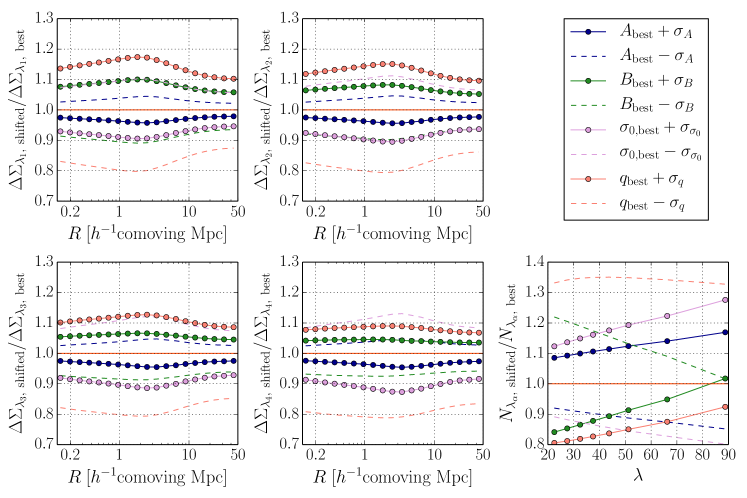
However, we make a further correction to the sample variance estimation. The cosmological model assumed in the actual measurement and the model fitting is the Planck cosmology, which is different from the WMAP cosmology (Hinshaw et al., 2013) used in making the mock catalogs of SDSS data. To correct for the systematic shift in the covariance amplitudes caused by this difference of cosmological models, we scale the sub-matrix of the sample-variance covariance matrix as follows. In particular this effect is significant for the abundance: the WMAP cosmology has smaller values of $\sigma_{8}$ and $\Omega_{\rm m0}$ than those in the Planck cosmology, and therefore gives about 7,000 redMaPPer clusters in each mock catalog, compared to 8,312 in the data. For the sub-covariance matrix involving the abundances, ${\bf C}^{\rm SV}(N_{\lambda_{\alpha}},N_{\lambda_{\alpha^{\prime}}})$, we use the formula in Hu & Kravtsov (2003) to correct for the cosmology difference. We first subtract $N_{\lambda_{\alpha}}^{\it WMAP}\delta^{K}_{\alpha\alpha^{\prime}}$ as the Poisson noise, where $N_{\lambda_{\alpha}}^{\it WMAP}$ is the average over the 108 realizations and $\delta^{K}_{\alpha\alpha^{\prime}}$ is Kronecker delta, from the sub-covariance matrix, and then multiply the remaining term by a factor of $(N_{\lambda_{\alpha}}^{\textit{Planck}}N_{\lambda_{\alpha^{\prime}}}^{\textit{Planck}})/(N_{\lambda_{\alpha}}^{\it WMAP}N_{\lambda_{\alpha^{\prime}}}^{\it WMAP})$ in each richness bin, where $N_{\lambda_{\alpha}}^{\textit{Planck}}$ is the best-fit model value from the crude covariance described in Section 4.2. After this correction, we add the Poisson term for Planck cosmology, $N^{\it Planck}_{\lambda_{\alpha}}\delta^{K}_{\alpha\alpha^{\prime}}$. Similarly, for the cross-covariance matrix, ${\bf C}^{\rm SV}(N_{\lambda_{\alpha}},\Delta\Sigma_{\lambda_{\beta}})$, we multiply a factor of $N_{\lambda_{\alpha}}^{\it Planck}/N_{\lambda_{\alpha}}^{\it WMAP}$ for the correction of the abundance. For the sub-covariance matrix involving the lensing profile $\Delta\Sigma_{\lambda_{\beta}}$, we multiply each component by a factor of $(\Delta\Sigma_{\lambda_{\beta}}^{\it Planck}/\Delta\Sigma_{\lambda_{\beta}}^{\it WMAP})$ for $R>1h^{-1}{\rm Mpc}$ with enough angular resolution in the mock catalogs. Here $\Delta\Sigma_{\lambda_{\beta}}^{\it WMAP}$ is the average over the 108 realizations and $\Delta\Sigma_{\lambda_{\beta}}^{\it Planck}$ is the best-fit model value from the crude covariance. However, since the shape noise gives a dominant contribution to the covariance involving $\Delta\Sigma_{\lambda_{\beta}}$, this correction for $\Delta\Sigma_{\lambda_{\beta}}$is not significant.

B.3. Random Covariance: ${\bf C}^{\rm R}$

The stacked cluster lensing is a cross-correlation of the number density fluctuation field of clusters with the matter perturbation. In analogous to the method in Landy & Szalay (1993), the cross-correlation can be measured by subtracting the stacked lensing profile around random points from that around the clusters. The stacked lensing around random catalogs is generally non-zero due to boundary effects of a general survey geometry. The use of the random subtraction corrects for these effects. Thus the use of the random catalogs in the lensing estimator reduces the covariance, as shown in Section 2.3 of Singh et al. (2017).

To create random catalogs, we randomly assign angular positions to each of the “real” SDSS redMaPPer clusters within the SDSS survey footprint (without masks) that is the same footprint of the mock catalog. In this way we generated 100 times the number of real redMaPPer clusters. Note that, by construction, the random catalogs have the same distributions of richness and redshift as those of the real clusters. We use the same random catalogs for all the 108 mock catalogs. We compute the covariance term of random points in equation (B1) as

$${\bf C}^{\rm R}(D_{i},D_{j})=\frac{1}{N_{\rm r}}\sum_{a=1}^{N_{\rm r}}[D^{\rm R}_{a,i}-\overline{D}{}^{\rm R}_{i}][D^{\rm R}_{a,j}-\overline{D}{}^{\rm R}_{j}],$$ (B6)

where $D^{\rm R}_{a,i}$ is the lensing measurement from the mock catalogs with shape noise around random points or the abundance measurement for the total area, in the $a$-th realization, and $\overline{D}{}^{\rm R}_{i}$ is the average over 108 realizations.

Appendix C Dependences of cluster observables on the parameters in mass-richness relation

To be self-contained within this paper, we here study the dependences of the abundance and the lensing profiles on model parameters in the mass-richness relation. Figure 18 shows the lensing profiles and the abundance in each richness bin when shifting each model parameter by an amount of the 68% CL interval around the best-fit value with fixing other parameters to the best-fit values for the sample of $20\leq\lambda\leq 100$ (see Table 3 for the values).

Appendix D The posterior distributions of cluster observables for the lensing or abundance alone

Figure 19.— The histogram in each panel shows the posterior distribution of the model lensing profile at a given radial bin for each richness cluster sample, which is computed from the MCMC chains when the mass-richness relation is constrained from the model comparison with the abundance information alone, as done in Figure 13. The vertical black dashed line denotes the model prediction for the best-fit model that reproduces the abundance. The shaded region shows the 16th and 84th percentiles of the posterior distribution. For comparison the red point with error bar denotes the measurement with the estimated error.

Figure 20.— Similarly to the previous figure, but the posterior distribution of the abundance in each richness bin, computed from the MCMC chains from the comparison with the lensing information alone, as done in Figure 14.

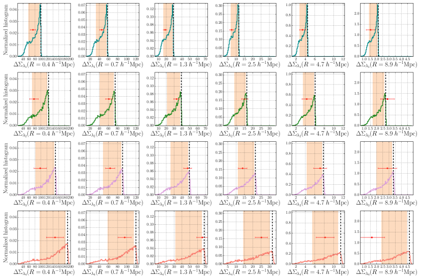
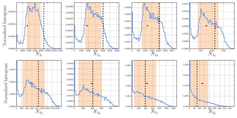
Figures 19 and 20 show the posterior distribution of cluster observables, the lensing profile or the abundance that are computed from the MCMC chains when the mass-richness relation is constrained from the model comparison with either alone of the abundance or the lensing information. These give a supplementary information to the results in Figures 13 and 14. Figure 19 shows that the lensing measurements in the lowest richness bin ($20<\lambda<30$) are systematically smaller than the posterior distributions from the abundance alone fitting result. Figure 20 also shows that the abundance measurements in the first and second richness bins ($20<\lambda<25$ and $25<\lambda<30$) are relatively small values compared to the posterior distributions from the lensing alone fitting result, although the significance is not very high. As discussed in Section 6.5, these results might be a signature of the residual systematics in the data (e.g. the projection effects at the low richness bins).

References

- Aihara et al. (2011) Aihara, H., et al. 2011, ApJS, 193, 29
- Aihara et al. (2017) —. 2017, PASJ, in press
- Bartelmann & Schneider (2001) Bartelmann, M., & Schneider, P. 2001, Phys. Rep., 340, 291
- Battaglia et al. (2016) Battaglia, N., et al. 2016, J. Cosmology Astropart. Phys, 8, 013
- Baxter et al. (2016) Baxter, E. J., Rozo, E., Jain, B., Rykoff, E., & Wechsler, R. H. 2016, MNRAS, 463, 205
- Behroozi et al. (2013) Behroozi, P. S., Wechsler, R. H., & Wu, H.-Y. 2013, ApJ, 762, 109
- Bernstein & Jarvis (2002) Bernstein, G. M., & Jarvis, M. 2002, The Astronomical Journal, 123, 583
- Busch & White (2017) Busch, P., & White, S. D. M. 2017, MNRAS, 470, 4767
- Clampitt et al. (2017) Clampitt, J., et al. 2017, MNRAS, 465, 4204
- Cohn et al. (2007) Cohn, J. D., Evrard, A. E., White, M., Croton, D., & Ellingson, E. 2007, MNRAS, 382, 1738
- Coupon et al. (2015) Coupon, J., et al. 2015, MNRAS, 449, 1352
- Dawson et al. (2013) Dawson, K. S., et al. 2013, AJ, 145, 10
- Diemer & Kravtsov (2014) Diemer, B., & Kravtsov, A. V. 2014, ApJ, 789, 1
- Dietrich et al. (2014) Dietrich, J. P., et al. 2014, MNRAS, 443, 1713
- Efron (1982) Efron, B. 1982, The Jackknife, the Bootstrap and other resampling plans
- Eke et al. (1996) Eke, V. R., Cole, S., & Frenk, C. S. 1996, MNRAS, 282
- Feldmann et al. (2006) Feldmann, R., et al. 2006, MNRAS, 372, 565
- Foreman-Mackey et al. (2013) Foreman-Mackey, D., Hogg, D. W., Lang, D., & Goodman, J. 2013, PASP, 125, 306
- Górski et al. (2005) Górski, K. M., Hivon, E., Banday, A. J., Wandelt, B. D., Hansen, F. K., Reinecke, M., & Bartelmann, M. 2005, ApJ, 622, 759
- Gruen et al. (2015) Gruen, D., Seitz, S., Becker, M. R., Friedrich, O., & Mana, A. 2015, MNRAS, 449, 4264
- Haiman et al. (2001) Haiman, Z., Mohr, J. J., & Holder, G. P. 2001, ApJ, 553, 545
- Hamana & Mellier (2001) Hamana, T., & Mellier, Y. 2001, MNRAS, 327, 169
- Hamilton (2000) Hamilton, A. J. S. 2000, MNRAS, 312, 257
- Hartlap et al. (2007) Hartlap, J., Simon, P., & Schneider, P. 2007, A&A, 464, 399
- Hikage et al. (2013) Hikage, C., Mandelbaum, R., Takada, M., & Spergel, D. N. 2013, MNRAS, 435, 2345
- Hikage et al. (2012) Hikage, C., Takada, M., & Spergel, D. N. 2012, MNRAS, 419, 3457
- Hinshaw et al. (2013) Hinshaw, G., et al. 2013, ApJS, 208, 19
- Hirata & Seljak (2003) Hirata, C., & Seljak, U. 2003, MNRAS, 343, 459
- Hoekstra et al. (2015) Hoekstra, H., Herbonnet, R., Muzzin, A., Babul, A., Mahdavi, A., Viola, M., & Cacciato, M. 2015, MNRAS, 449, 685
- Hu & Kravtsov (2003) Hu, W., & Kravtsov, A. V. 2003, ApJ, 584, 702
- Jimeno et al. (2017) Jimeno, P., Broadhurst, T., Lazkoz, R., Angulo, R., Diego, J.-M., Umetsu, K., & Chu, M.-c. 2017, MNRAS, 466, 2658
- Johnston et al. (2007) Johnston, D. E., et al. 2007, ArXiv e-prints:0709.1159
- Kitayama & Suto (1997) Kitayama, T., & Suto, Y. 1997, ApJ, 490, 557
- Landy & Szalay (1993) Landy, S. D., & Szalay, A. S. 1993, ApJ, 412, 64
- Lewis et al. (2000) Lewis, A., Challinor, A., & Lasenby, A. 2000, ApJ, 538, 473
- Lima & Hu (2005) Lima, M., & Hu, W. 2005, Phys. Rev. D, 72, 043006
- Mandelbaum et al. (2013) Mandelbaum, R., Slosar, A., Baldauf, T., Seljak, U., Hirata, C. M., Nakajima, R., Reyes, R., & Smith, R. E. 2013, MNRAS, 432, 1544
- Mandelbaum et al. (2005) Mandelbaum, R., et al. 2005, MNRAS, 361, 1287
- Melchior et al. (2017) Melchior, P., et al. 2017, MNRAS, 469, 4899
- Miyatake et al. (2016) Miyatake, H., More, S., Takada, M., Spergel, D. N., Mandelbaum, R., Rykoff, E. S., & Rozo, E. 2016, Physical Review Letters, 116, 041301
- Miyatake et al. (2015) Miyatake, H., et al. 2015, ApJ, 806, 1
- More et al. (2015) More, S., Miyatake, H., Mandelbaum, R., Takada, M., Spergel, D. N., Brownstein, J. R., & Schneider, D. P. 2015, ApJ, 806, 2
- More et al. (2016) More, S., et al. 2016, ApJ, 825, 39
- Nakajima et al. (2012) Nakajima, R., Mandelbaum, R., Seljak, U., Cohn, J. D., Reyes, R., & Cool, R. 2012, MNRAS, 420, 3240
- Navarro et al. (1996) Navarro, J. F., Frenk, C. S., & White, S. D. M. 1996, ApJ, 462, 563
- Nishimichi et al. (2009) Nishimichi, T., et al. 2009, PASJ, 61, 321
- Oguri & Takada (2011) Oguri, M., & Takada, M. 2011, Phys. Rev. D, 83, 023008
- Oguri et al. (2017) Oguri, M., et al. 2017, PASJ, in press
- Okabe et al. (2013) Okabe, N., Smith, G. P., Umetsu, K., Takada, M., & Futamase, T. 2013, ApJ, 769, L35
- Okabe et al. (2010) Okabe, N., Takada, M., Umetsu, K., Futamase, T., & Smith, G. P. 2010, PASJ, 62, 811
- Okumura et al. (2017) Okumura, T., Takada, M., More, S., & Masaki, S. 2017, MNRAS, 469, 459
- Olive et al. (2014) Olive, K. A., et al. 2014, Chin. Phys. C, 38, 090001
- Planck Collaboration et al. (2016a) Planck Collaboration et al. 2016a, A&A, 594, A13
- Planck Collaboration et al. (2016b) —. 2016b, A&A, 594, A24
- Reyes et al. (2012) Reyes, R., Mandelbaum, R., Gunn, J. E., Nakajima, R., Seljak, U., & Hirata, C. M. 2012, MNRAS, 425, 2610
- Rozo & Rykoff (2014) Rozo, E., & Rykoff, E. S. 2014, ApJ, 783, 80
- Rozo et al. (2015a) Rozo, E., Rykoff, E. S., Bartlett, J. G., & Melin, J.-B. 2015a, MNRAS, 450, 592
- Rozo et al. (2015b) Rozo, E., Rykoff, E. S., Becker, M., Reddick, R. M., & Wechsler, R. H. 2015b, MNRAS, 453, 38
- Rozo et al. (2009) Rozo, E., et al. 2009, ApJ, 703, 601
- Rozo et al. (2010) —. 2010, ApJ, 708, 645
- Rykoff et al. (2012) Rykoff, E. S., et al. 2012, ApJ, 746, 178
- Rykoff et al. (2014) —. 2014, ApJ, 785, 104
- Rykoff et al. (2016) —. 2016, ApJS, 224, 1
- Saro et al. (2015) Saro, A., et al. 2015, MNRAS, 454, 2305
- Sheldon et al. (2004) Sheldon, E. S., et al. 2004, AJ, 127, 2544
- Shirasaki et al. (2015) Shirasaki, M., Hamana, T., & Yoshida, N. 2015, MNRAS, 453, 3043
- Shirasaki et al. (2017) Shirasaki, M., Takada, M., Miyatake, H., Takahashi, R., Hamana, T., Nishimichi, T., & Murata, R. 2017, MNRAS, 470, 3476
- Simet et al. (2017) Simet, M., McClintock, T., Mandelbaum, R., Rozo, E., Rykoff, E., Sheldon, E., & Wechsler, R. H. 2017, MNRAS, 466, 3103
- Singh et al. (2017) Singh, S., Mandelbaum, R., Seljak, U., Slosar, A., & Vazquez Gonzalez, J. 2017, MNRAS, 471, 3827
- Spergel et al. (2013) Spergel, D., et al. 2013, ArXiv e-prints:1305.5425
- Springel (2005) Springel, V. 2005, MNRAS, 364, 1105
- Takada & Bridle (2007) Takada, M., & Bridle, S. 2007, New Journal of Physics, 9, 446
- Takada & Hu (2013) Takada, M., & Hu, W. 2013, Phys. Rev. D, 87, 123504
- Takada & Spergel (2014) Takada, M., & Spergel, D. N. 2014, MNRAS, 441, 2456
- Takahashi et al. (2017) Takahashi, R., Hamana, T., Shirasaki, M., Namikawa, T., Nishimichi, T., Osato, K., & Shiroyama, K. 2017, ApJ, 850, 24
- van Uitert et al. (2016) van Uitert, E., Gilbank, D. G., Hoekstra, H., Semboloni, E., Gladders, M. D., & Yee, H. K. C. 2016, A&A, 586, A43
- Vikhlinin et al. (2009) Vikhlinin, A., et al. 2009, ApJ, 692, 1060
- Weinberg et al. (2013) Weinberg, D. H., Mortonson, M. J., Eisenstein, D. J., Hirata, C., Riess, A. G., & Rozo, E. 2013, Phys. Rep., 530, 87
- White et al. (1993) White, S. D. M., Efstathiou, G., & Frenk, C. S. 1993, MNRAS, 262, 1023
- Zu et al. (2017) Zu, Y., Mandelbaum, R., Simet, M., Rozo, E., & Rykoff, E. S. 2017, MNRAS, 470, 551