Negative association, ordering and convergence of resampling methods

Abstract

We study convergence and convergence rates for resampling schemes. Our first main result is a general consistency theorem based on the notion of negative association, which is applied to establish the almost sure weak convergence of measures output from Kitagawa’s (1996) stratified resampling method. Carpenter et al’s (1999) systematic resampling method is similar in structure but can fail to converge depending on the order of the input samples. We introduce a new resampling algorithm based on a stochastic rounding technique of Srinivasan, (2001), which shares some attractive properties of systematic resampling, but which exhibits negative association and therefore converges irrespective of the order of the input samples. We confirm a conjecture made by Kitagawa, (1996) that ordering input samples by their states in $\mathbb{R}$ yields a faster rate of convergence; we establish that when particles are ordered using the Hilbert curve in $\mathbb{R}^{d}$, the variance of the resampling error is ${\scriptscriptstyle\mathcal{O}}(N^{-(1+1/d)})$ under mild conditions, where $N$ is the number of particles. We use these results to establish asymptotic properties of particle algorithms based on resampling schemes that differ from multinomial resampling.

Keywords: Negative association, resampling, particle filtering

1 Introduction

A resampling scheme is a randomized procedure that takes as input random samples $X^{n}$ with nonnegative weights $W^{n}\geq 0$, $n=1,\ldots,N$, such that $\sum_{n=1}^{N}W^{n}=1$, and returns as an output resampled variables $X^{A^{n}}$, where $A^{n}$ is a random index in $\{1,\ldots,N\}$, such that, in some sense,

$$\frac{1}{N}\sum_{n=1}^{N}\delta(X^{A^{n}})\approx\sum_{n=1}^{N}W^{n}\delta({X^{n}}).$$ (1)

Here $\delta(x)$ denotes the Dirac measure at point $x$ (this slightly unconventional notation will make our equations more readable).

Resampling appears in various statistical procedures. The present work is primarily motivated by resampling within Sequential Monte Carlo methods, also known as particle filters (Doucet et al.,, 2001). Particle filters approximate recursively a sequence of probability distributions by propagating N ‘particles’ through weighting, resampling and mutation steps. The resampling steps play a crucial role in stabilizing the Monte Carlo error over time (Gordon et al.,, 1993). In particular, without resampling, the largest normalised weight of the particle sample converges quickly to one as the number of iterations increases (Del Moral and Doucet,, 2003). This means that most of the computational effort is wasted on particles that contribute little to the end results.

Resampling also appears in survey sampling under the name of ‘unequal probability sampling’ (Tillé,, 2006), but in a context slightly different from the one we consider in this paper. In survey sampling only $M<N$ ‘units’ are selected and the object of interest after the (re)sampling operation, the Horvitz-Thompson empirical process (HTEP, see e.g. Bertail et al.,, 2017) is another un-normalized weighted sum of Dirac measures. Adapting the statement and the assumptions of our first main result, Theorem 1 in Section 2, in order to study the asymptotic behaviour of the HTEP is possible but beyond the scope of this paper. Yet another statistical procedure where resampling appears is the the weighted bootstrap (Barbe and Bertail,, 1995).

There are various existing resampling methods. Multinomial resampling is perhaps the simplest technique, where given the weights, the indices $A^{n}$ are generated conditionally independently from the finite distribution that assigns probability $W^{n}$ to outcome $n$. In particle filtering it is common practice to replace multinomial resampling with techniques which are computationally faster and empirically more accurate. However, these advanced resampling techniques are generally not straightforward to analyse because they induce complicated dependence between output samples, and various aspects of their behaviour are still not understood.

Following definitions and an account of what is known about existing resampling techniques, our first main result, Theorem 1 in Section 2, is a general consistency result for resampling based on the notion of negative association (Joag-Dev and Proschan,, 1983). An application of this theorem gives, to our knowledge, the first proof of almost sure weak convergence of the random probability measures output from the stratified resampling method of Kitagawa, (1996). A notable feature of Theorem 1 is that, although its assumptions do not require the input particles to be algorithmically ordered in a particular way, its proof involves establishing a necessary and sufficient condition for almost sure weak convergence involving ordering using the Hilbert space-filling curve. Here we build on Gerber and Chopin, (2015), who used the Hilbert curve to derive and analyse a quasi-Monte Carlo version of sequential Monte Carlo samplers.

The systematic resampling method of Carpenter et al., (1999), which involves a sampling technique first proposed by Madow and Madow, (1944), is a very popular and computationally cheap resampling technique, with the property that the number of offspring of any sample with weight $W$ in a population of size $N$ is with probability $1$ either $\left\lfloor NW\right\rfloor$ or $\left\lfloor NW\right\rfloor+1$. However, depending on the order of the input particles, the error variance for systematic resampling can fail to converge to zero as $N\to+\infty$, see Douc et al., (2005) and L’Ecuyer and Lemieux, (2000). We complement this insight by providing a counter-example to almost sure weak convergence. We then introduce a new resampling method, called Srinivasan Sampling Process (SSP) resampling, which corrects this deficiency: it also has the property that offspring numbers are of the form either $\left\lfloor NW\right\rfloor$ or $\left\lfloor NW\right\rfloor+1$, but it provably converges irrespective of the order of input particles, by another application of our Theorem 1.

Kitagawa, (1996) conjectured that in the case that the state-space is $\mathbb{R}$, ordering the particles input to stratified resampling according to their states leads to faster convergence. In particular, he suggested that the integrated square error between empirical cdf’s before and after resampling behaves as $\mathcal{O}(N^{-2})$, compared to the standard Monte Carlo rate $\mathcal{O}(N^{-1})$ in the un-ordered case. We confirm this conjecture by proving, under mild conditions, that for stratified resampling on state-space $\mathbb{R}^{d}$ with input particles ordered by their states using the Hilbert curve, the variance of the resampling error is ${\scriptscriptstyle\mathcal{O}}(N^{-(1+1/d)})$. Kitagawa also examined the behaviour of a deterministic resampling scheme; we identify the variant of it which is optimal in terms of the Kolmogorov metric when the state-space is $\mathbb{R}$. We also prove the almost sure weak consistency of stratified and systematic when the particles are Hilbert-ordered.

Finally, we discuss the implications of our results on particle filtering. In particular, we show that particle estimates are consistent when resampling schemes such as e.g. SSP or stratified resampling are used. In addition, we show that the ordered version of stratified resampling dominates other resampling schemes in terms of asymptotic variance of particle estimates.

All the proofs are gathered in the supplementary materials.

2 Preliminaries

2.1 Notation and conventions

Let $\mathcal{X}$ be an open subset of $\mathbb{R}^{d}$, $\mathbb{X}$ its Borel $\sigma$-algebra, $\mathcal{P}(\mathcal{X})$ the set of probability measures on $(\mathcal{X},\mathbb{X})$, $\mathcal{P}_{b}(\mathcal{X})\subset\mathcal{P}(\mathcal{X})$ the subset of measures in $\mathcal{P}(\mathcal{X})$ which admit a continuous and bounded density with respect to $\lambda_{d}$, the Lebesgue measure on $\mathcal{X}$, and $\mathcal{P}_{f}(\mathcal{X})\subset\mathcal{P}(\mathcal{X})$ the subset of measures in $\mathcal{P}(\mathcal{X})$ whose support is a finite set.

For integers $1\leq a\leq b$, we will often use the index shorthands $z_{a:b}=(z_{a},\dots,z_{b})$ and $z^{a:b}=(z^{a},\dots,z^{b})$, and let $1:N=\{1,\ldots,N\}$.

For any measurable mapping $\varphi$ from $(\mathcal{X},\mathbb{X})$ to some measurable space $(\mathcal{Y},\mathbb{Y})$ and a probability measure $\pi\in\mathcal{P}(\mathcal{X})$, we write $\pi_{\varphi}$ for the pushforward of $\pi$ by $\varphi$. The set of continuous and bounded functions on $\mathcal{X}$ is denoted by $\mathcal{C}_{b}(\mathcal{X})$ and we use the symbol “$\xRightarrow{\text{w}}$” to denote weak convergence; that is, for sequence $(\pi^{N})_{N\geq 1}$ in $\mathcal{P}(\mathcal{X})$ and $\pi\in\mathcal{P}(\mathcal{X})$,

$$\pi^{N}\xRightarrow{\text{w}}\pi\quad\Leftrightarrow\quad\lim_{N\rightarrow+\infty}\pi^{N}(\varphi)=\pi(\varphi),\quad\forall\varphi\in\mathcal{C}_{b}(\mathcal{X}).$$

Throughout the paper we consider a fixed probability space $(\Omega,\mathcal{F},\mathbb{P})$ on which all random variables are defined. With $\mathcal{B}([0,1]^{\mathbb{N}})$ denoting the Borel $\sigma$-algebra on $[0,1]^{\mathbb{N}}$, let $U=(U_{1},U_{2},\ldots)$ be a $([0,1]^{\mathbb{N}},\mathcal{B}([0,1]^{\mathbb{N}}))$-valued random variable on $(\Omega,\mathcal{F},\mathbb{P})$, such that $\mathbb{P}$ makes $(U_{1},U_{2},\ldots)$ independent of each other and all other random variables, and such that each $U_{i}$ is distributed uniformly on $[0,1]$.

We note that one can choose a countable subset of $\mathcal{C}_{b}(\mathcal{X})$ that completely determines weak convergence, hence for random measures $(\pi^{N})_{N\geq 1}$, the event $\{\pi^{N}\xRightarrow{\text{w}}\pi\}$ is measurable.

For $\pi\in\mathcal{P}(\mathcal{X})$, we denote by $\pi(\varphi)$ the expectation $\int_{\mathcal{X}}\varphi(x)\pi(\mathrm{d}x)$, and for a random variable $Z=(Z_{1},\ldots,Z_{d})$ whose distribution is $\pi$ we denote by $F_{\pi}(a)=\mathbb{P}(Z_{1}\leq a_{1},\ldots,Z_{d}\leq a_{d})$, $a=(a_{1},\ldots,a_{d})$, its CDF (cumulative distribution function) and, when $d=1$, by $F^{-}_{\pi}$ its generalized inverse: $F^{-}_{\pi}(u)=\inf\{x:\,F_{\pi}(x)\geq u\}$.

For each $N\geq 1$ we consider a distinguished collection of random variables $\zeta^{N}=(X^{n,N},W^{n,N})_{n=1}^{N}$, with each $X^{n,N}$ valued in $\mathcal{X}$, each $(W^{n,N})_{n=1}^{N}$ valued in $\mathbb{R}_{+}$, and such that $\mathbb{P}$-a.s., $\sum_{n=1}^{N}W^{n,N}=1$. When no confusion may arise, we suppress dependence on $N$ and write $\zeta^{N}=(X^{n},W^{n})_{n=1}^{N}$. We associate with $\zeta^{N}$ the random measure $\pi^{N}=\sum_{n=1}^{N}W^{n}\delta(X^{n})$, the (random) CDF

$$F_{N}(n)=\sum_{m=1}^{N}W^{m}\mathds{1}(m\leq n),\quad n\in 1:N,$$

and its inverse is denoted $F_{N}^{-}$.

To lighten notation we shall write $\mathbb{P}_{\zeta^{N}}(\cdot)$, $\mathbb{E}_{\zeta^{N}}[\cdot]$, $\mathrm{Var}_{\zeta^{N}}[\cdot]$, $\mathrm{Cov}_{\zeta^{N}}[\cdot,\cdot]$ for conditional probability, expectation, variance and covariance given $\zeta^{N}$.

Let $\mathcal{Z}^{N}=\{(x,w)\in\mathcal{X}^{N}\times\mathbb{R}_{+}^{N}:\,\sum_{n=1}^{N}w_{n}=1\}$ and define the disjoint union $\mathcal{Z}\coloneqq\bigcup_{N=1}^{+\infty}\mathcal{Z}^{N}$. So we may think of $\zeta^{N}$ as a random point in $\mathcal{Z}^{N}$, and hence $\mathcal{Z}$.

Definition 1.

$\mathcal{X}\subseteq\mathbb{R}^{d}$ is said to be cubifiable if there exist measurable sets $\mathcal{X}_{i}\subseteq\mathbb{R}$, $i=1,\dots,d$, such that

1. $\mathcal{X}=\times_{i=1}^{d}\mathcal{X}_{i}$;

2. For any $i\in 1:d$, there exists a $C^{1}$-diffeomorphism $\psi_{i}:\mathcal{X}_{i}\rightarrow(0,1)$ which is strictly increasing on $\mathcal{X}_{i}$.

We shall write $\psi(x)=(\psi_{1}(x_{1}),\ldots,\psi_{d}(x_{d}))$, $x=x_{1:d}\in\mathcal{X}$, the resulting $C^{1}$-diffeomorphism from $\mathcal{X}$ into $(0,1)^{d}$.

We recall the reader that function $\psi:\mathcal{X}\rightarrow(0,1)^{d}$ is a $C^{1}$-diffeomorphism if it is a bijection and its inverse $\psi^{-1}:(0,1)^{d}\rightarrow\mathcal{X}$ is continuously differentiable. In what follows, for a cubifiable set $\mathcal{X}$ we denote by $\mathcal{D}(\mathcal{X})$ the set of all $C^{1}$-diffeomorphisms from $\mathcal{X}$ into $(0,1)^{d}$ that verify the conditions of Definition 1.

Cubifiable sets are sets that can be written as $\mathcal{X}=\times_{i=1}^{d}(a_{i},b_{i})$ for some $a_{i},b_{i}\in\mathbb{R}\cup\{-\infty,+\infty\}$. The point of these sets is to be able to work ‘as if’ $\mathcal{X}=(0,1)^{d}$. The hypercube $(0,1)^{d}$ will play a key role below because the Hilbert space-filling curve, which is essential in this work, is defined on this hypercube.

Most of the results presented below assume that the limiting distribution $\pi$ admits a continuous and bounded density. Consequently, to work ‘as if’ $\mathcal{X}=(0,1)^{d}$ we will often assume that $\pi$ belongs to

$$\widetilde{\mathcal{P}}_{b}(\mathcal{X})=\big{\{}\pi\in\mathcal{P}_{b}(\mathcal{X}):\,\exists\psi\in\mathcal{D}(\mathcal{X})\text{ s.t. }\pi_{\psi}\in\mathcal{P}_{b}((0,1)^{d})\Big{\}}.$$

The following result provides a sufficient condition to have $\pi\in\widetilde{\mathcal{P}}_{b}(\mathcal{X})$. We denote by $p_{\pi}$ the density (w.r.t. $\lambda_{d}$) of $\pi\in\mathcal{P}_{b}(\mathcal{X})$ and, for $I\subset 1:d$, we write $x_{I}=(x_{i},\,i\in I)$ and $x_{\setminus I}=(x_{i},\,i\not\in I)$.

Lemma 1.

Let $\mathcal{X}$ be a cubifiable set, $\delta>0$ and $\pi\in\mathcal{P}_{b}(\mathcal{X})$ such that $\forall I\subseteq 1:d$ and $\forall x_{\setminus I}\in\times_{i\not\in I}\mathcal{X}_{i}$ we have $\sup_{x_{I}\in\times_{i\in I}\mathcal{X}_{i}}p_{\pi}(x)\prod_{i\in I}|x_{i}|^{1+\delta}\leq C$ for some $C<+\infty$. Then $\pi\in\widetilde{\mathcal{P}}_{b}(\mathcal{X})$.

Recall that $\sup_{x\in\mathbb{R}}p_{\pi}(x)|x|<+\infty$ for any $\pi\in\mathcal{P}_{b}(\mathbb{R})$. Therefore, as $\delta>0$ is arbitrary in the lemma, very few extra conditions on the tails of $\pi\in\mathcal{P}_{b}(\mathbb{R})$ are needed in order to have $\pi\in\widetilde{\mathcal{P}}_{b}(\mathbb{R})$ when $d=1$. When $d>1$, assuming that $\pi\in\widetilde{\mathcal{P}}_{b}(\mathbb{R}^{d})$ is more restrictive since the lemma requires some uniformity in the behaviour of tails. However, we note that members of $\widetilde{\mathcal{P}}_{b}(\mathbb{R}^{d})$ may not have a first moment and therefore the sufficient condition of Lemma 1 appears to be quite weak.

2.2 Resampling schemes: definitions and properties

Definition 2.

A resampling scheme is a mapping $\rho:[0,1]^{\mathbb{N}}\times\mathcal{Z}\rightarrow\mathcal{P}_{f}(\mathcal{X})$ such that, for any $N\geq 1$ and $z=(x^{n},w^{n})_{n=1}^{N}\in\mathcal{Z}^{N}$,

$$\rho(u,z)=\frac{1}{N}\sum_{n=1}^{N}\delta(x^{a_{N}^{n}(u,z)}),$$

where for each $n$, $a_{N}^{n}:[0,1]^{\mathbb{N}}\times\mathcal{Z}^{N}\to 1:N$ is a measurable function.

Given $u\in[0,1]^{\mathbb{N}}$, the mapping $\rho(u,\cdot)$ therefore takes as input a weighted point set $z=(x^{n},w^{n})_{n=1}^{N}$, selects $N$ indices $(a_{N}^{n}(u,z))_{n=1}^{N}$ in the set $1:N$ and returns a probability measure on $(x^{n})_{n=1}^{N}$ with the property that each $x^{a_{N}^{n}(u,z)}$ has weight $N^{-1}$.

Instances of the function $a_{N}^{n}$ are given below. We shall use the shorthands $\rho(z)$ for the random measure $\rho(U,z)$, $z\in{\mathcal{Z}^{N}}$, and $A^{n}$ for the random indices $a_{N}^{n}(U,\zeta^{N})$. Introducing the quantities,

$$\#^{n}(u,z)=\mathrm{card}\{i\in 1:N\;\;\mathrm{s.t.}\;\;a_{N}^{i}(u,z)=n\},\,\Delta_{\rho,z}^{n}=\#^{n}(U,z)-Nw^{n},$$ (2)

a resampling scheme $\rho$ is said to be unbiased if, for any $N\geq 1$, $n\in 1:N$ and $z\in\mathcal{Z}^{N}$,

$$\mathbb{E}[\Delta_{\rho,z}^{n}]=0.$$

We now define the resampling schemes of primary interest in this work.

• Multinomial resampling: $\rho_{\mathrm{multi}}$ such that

  $$a_{N}^{n}(u,\zeta^{N})=F_{N}^{-}(u_{n}).$$

  In this case the $a^{n}_{N}(U,\zeta^{N})$ are i.i.d. (independent and identically distributed) draws from the distribution which assigns probability $W^{n}$ to outcome $n$.

• Stratified resampling: $\rho_{\mathrm{strat}}$ such that

  $$a_{N}^{n}(u,\zeta^{N})=F_{N}^{-}\left(\frac{n-1+u_{n}}{N}\right).$$

• Systematic resampling: $\rho_{\mathrm{syst}}$ such that

  $$a_{N}^{n}(u,\zeta^{N})=F_{N}^{-}\left(\frac{n-1+u_{1}}{N}\right).$$

The following definition captures the notion of almost sure weak convergence of the random measures $(\pi^{N})_{N\geq 1}$ which we shall study and is similar to condition (9) in (Crisan and Doucet,, 2002).

Definition 3.

Let $\mathcal{P}_{0}\subseteq\mathcal{P}(\mathcal{X})$. Then, we say that a resampling scheme $\rho:[0,1]^{\mathbb{N}}\times\mathcal{Z}\rightarrow\mathcal{P}_{f}(\mathcal{X})$ is $\mathcal{P}_{0}$-consistent if, for any $\pi\in\mathcal{P}_{0}$ and $(\zeta^{N})_{N\geq 1}$ such that $\pi^{N}\xRightarrow{\text{w}}\pi$, $\mathbb{P}$-a.s., one has

$$\rho(\zeta^{N})\xRightarrow{\text{w}}\pi,\quad\mathbb{P}-\mbox{a.s.}$$

It is well known that multinomial, stratified and systematic resampling are unbiased. An account of various properties of these methods can be found in Douc et al., (2005).

Crisan and Doucet, (2002, Lemma 2) shows that multinomial resampling is $\mathcal{P}(\mathcal{X})$-consistent for any measurable set $\mathcal{X}\subseteq\mathbb{R}^{d}$.

It is easy to show (Stein,, 1987; Douc et al.,, 2005) that stratified resampling dominates multinomial resampling in terms of variance, i.e.,

$$\mathrm{Var}\left[\rho_{\mathrm{strat}}(z)(\varphi)\right]\leq\mathrm{Var}\left[\rho_{\mathrm{multi}}(z)(\varphi)\right],\quad\forall z\in\mathcal{Z}$$

for any measurable $\varphi:\mathcal{X}\rightarrow\mathbb{R}$. Similar results are harder to derive for systematic resampling, owing to the strong dependencies between the resampled indices. However, it is known (Douc et al.,, 2005) that the variance of $\rho_{\mathrm{syst}}(\zeta^{N})(\varphi)$ may not converge to $0$ as $N\rightarrow+\infty$ (see also L’Ecuyer and Lemieux,, 2000, for an explanation of this phenomenon).

3 Convergence of resampling schemes based on negative association

3.1 A general consistency result

Before stating the main result of this section we recall the definition of negatively associated (NA) random variables (Joag-Dev and Proschan,, 1983).

Definition 4.

A collection of random variables $(Z^{n})_{n=1}^{N}$ are negatively associated if, for every pair of disjoint subsets $I_{1}$ and $I_{2}$ of $\{1,\dots N\}$,

$$\mathrm{Cov}\Big{(}\varphi_{1}\big{(}Z^{n},n\in I_{1}\big{)},\,\varphi_{2}\big{(}Z^{n},n\in I_{2}\big{)}\Big{)}\leq 0$$

for all coordinatewise non-decreasing functions $\varphi_{1}$ and $\varphi_{2}$ such that for $k\in\{1,2\}$, $\varphi_{k}:\mathbb{R}^{|I_{k}|}\rightarrow\mathbb{R}$, and such that the covariance is well-defined.

Theorem 1.

Let $\mathcal{X}$ be a cubifiable set and $\rho$ be an unbiased resampling scheme such that the following conditions hold:

1. For any $N\geq 1$ and $z\in\mathcal{Z}^{N}$, the random variables $(\#^{n}(U,z))_{n=1}^{N}$ are negatively associated;

2. There exists a sequence $(r_{N})_{N\geq 1}$ of non-negative real numbers such that $r_{N}={\scriptscriptstyle\mathcal{O}}(N/\log N)$ and, for $N$ large enough,

   $$\sup_{z\in\mathcal{Z}^{N}}\sum_{n=1}^{N}\mathbb{E}\big{[}(\Delta_{\rho,z}^{n})^{2}\big{]}\leq r_{N}\,N,\quad\sum_{N=1}^{\infty}\sup_{z\in\mathcal{Z}^{N}}\mathbb{P}\Big{(}\max_{n\in 1:N}\big{|}\Delta_{\rho,z}^{n}\big{|}>r_{N}\Big{)}<+\infty.$$

Then, $\rho$ is $\widetilde{\mathcal{P}}_{b}(\mathcal{X})$-consistent.

The strategy of the proof is the following. In a first step, we show that when $\sigma_{N}^{*}$ is a permutation of $1:N$ which corresponds to ordering input particles using the Hilbert space filling curve (details of which we postpone to Section 4), the resampling scheme $\rho$ is $\widetilde{\mathcal{P}}_{b}(\mathcal{X})$-consistent if and only if

$$\lim_{N\rightarrow+\infty}\max_{m\in 1:N}\big{|}\sum_{n=1}^{m}\Delta_{\rho,z_{N}}^{\sigma_{N}^{*}(n)}\big{|}=0,\quad\mathbb{P}-a.s.$$ (3)

for any sequence $(z_{N})_{N\geq 1}$ with $z_{N}\in\mathcal{Z}^{N}$. In a second step, we show that the hypotheses ($H_{1}$) and ($H_{2}$) are sufficient to establish (3), via a maximal inequality for negatively associated random variables due to Shao, (2000). We stress here that the permutation $\sigma_{N}^{*}$ is introduced solely as a device in the proof; there is no assumption in Theorem 1 that the input particles are algorithmically sorted in any particular way. The reader should note, in fact, that ($H_{1}$) must hold for all $z$, and ($H_{2}$) is uniform in $z$, and hence all permutations of the input particles.

3.2 Discussion of ($H_{1}$) and ($H_{2}$)

From the definition of $\#^{n}(U,z)$ given in (2) it follows that $\sum_{n=1}^{N}\#^{n}(U,z)=N$, $\mathbb{P}$-as. Intuitively, this constraint suggests that at least some random variables in the set $(\#^{n}(U,z))_{n=1}^{N}$ are negatively correlated. ($H_{1}$) may be understood as imposing that all these random variables are negatively correlated.

($H_{2}$) alone is not sufficient to guarantee the consistency of an unbiased resampling scheme. If a resampling scheme $\rho$ violates ($H_{1}$) then it is indeed possible to find examples where the offspring numbers are positively correlated in a way that, with positive probability, prevents the limit in (3) from being zero. The next result formalizes this assertion in the context of systematic resampling. Its proof involves a somewhat technical construction of a counter-example.

Proposition 1.

The systematic resampling scheme $\rho_{\mathrm{syst}}$ is unbiased, satisfies ($H_{2}$) with $r_{N}=1$ but is not $\widetilde{\mathcal{P}}_{b}(\mathcal{X})$-consistent.

On the other hand, ($H_{1}$) alone is not enough to guarantee consistency. If we consider the resampling scheme $\rho$ such that $\#^{n}(U,z)=N$ with probability $w^{n}$, it is easily checked $\rho$ is unbiased and ($H_{1}$) holds, but this resampling scheme is obviously not $\widetilde{\mathcal{P}}_{b}(\mathcal{X})$-consistent. ($H_{2}$) rules out this kind of situation via constraints on the second moments and negligibility of the deviations of the offspring numbers $(\#^{n}(U,z))_{n=1}^{N}$ from their respective means $(Nw^{n})_{n=1}^{N}$.

3.3 Some comments about systematic resampling

Systematic resampling has the property that $\#^{n}(U,z)$ is either $\lfloor Nw^{n}\rfloor$ or $\lfloor Nw^{n}\rfloor+1$, $\mathbb{P}$-a.s., hence $|\Delta_{\rho_{\mathrm{syst}},z^{N}}^{n}|\leq 1$, $\mathbb{P}$-a.s., so that ($H_{2}$) holds with $r_{N}=1$ as stated in Proposition 1.

A corollary of this latter is that systematic resampling violates ($H_{1}$). A simple way to establish this result is to take a $z\in\mathcal{Z}^{N}$ such that we have $Nw^{n}-\lfloor Nw^{n}\rfloor=1/2$ for $n=1,\dots,3$. Then,

$$\mathbb{P}\big{(}\#^{1}(U,z)=\#^{3}(U,z)=1\big{)}=\frac{1}{2}>\mathbb{P}\big{(}\#^{1}(U,z)=1)\mathbb{P}(\#^{3}(U,z)=1\big{)}=\frac{1}{4}$$

showing that the collection of random variables $(\#^{n}(U,z))_{n=1}^{N}$ is not NA.

To overcome the lack of consistency (in the sense of Definition 3) of systematic resampling we introduce below (Section 3.4.3) a new resampling scheme, named SSP (for Srinivasan Sampling Process) resampling, which both satisfies the NA condition ($H_{1}$) and shares the property of systematic resampling that $|\Delta_{\rho_{\mathrm{syst}},z^{N}}^{n}|\leq 1$ for all $n\in 1:N$, $\mathbb{P}$-a.s., so that ($H_{2}$) also holds with $r_{N}=1$ for this new resampling scheme.

3.4 Applications of Theorem 1

3.4.1 Multinomial resampling

As already mentioned, it is a known result that multinomial resampling is $\mathcal{P}(\mathcal{X})$-consistent for any measurable $\mathcal{X}\subseteq\mathbb{R}^{d}$ (Crisan and Doucet,, 2002, Lemma 2). Theorem 1 may be applied to obtain a similar result.

Corollary 1.

Let $\mathcal{X}$ be a cubifiable set. Then, the resampling scheme $\rho_{\mathrm{multi}}$ verifies conditions ($H_{1}$) and ($H_{2}$) of Theorem 1 and is therefore $\widetilde{\mathcal{P}}_{b}(\mathcal{X})$-consistent.

Condition ($H_{1}$) holds for multinomial resampling as shown by Joag-Dev and Proschan, (1983) while ($H_{2}$) is verified using properties of the binomial distribution and Hoeffding’s inequality.

For similar reasons, the conditions of Theorem 1 are also satisfied by the residual resampling scheme of Liu and Chen, (1998).

3.4.2 Stratified resampling

To the best of our knowledge the following corollary of Theorem 1 is the first almost sure weak convergence result for Kitagawa’s (1996) stratified resampling scheme.

Corollary 2.

Let $\mathcal{X}$ be a cubifiable set. Then the resampling scheme $\rho_{\mathrm{strat}}$ verifies conditions ($H_{1}$) and ($H_{2}$) of Theorem 1 and is therefore $\widetilde{\mathcal{P}}_{b}(\mathcal{X})$-consistent.

Verifying ($H_{1}$) in this situation involves the observation that stratified resampling is a “Balls and Bins” experiment (Dubhashi and Ranjan,, 1998) in which $N$ balls are independently thrown into $N$ bins, the total number of balls occupying the $n$th bin is $\#^{n}(U,z)$, and where the probability of falling in a given bin varies across balls, due to the stratified nature of the sampling. The fact that ($H_{1}$) holds is then a direct consequence of Theorem 14 in Dubhashi and Ranjan, (1998), which establishes the NA of occupancy numbers in a slightly more general balls and bins problem where the number of balls is not necessarily equal to the number of bins. ($H_{2}$) holds because $|\Delta_{\rho_{\mathrm{strat}},z}|\leq 2$, $\mathbb{P}$-a.s.

It is worth noting that the conditions of Theorem 1 are also satisfied by the stratified version of the residual resampling scheme of Liu and Chen, (1998), where the multinomial resampling part is replaced by a stratified resampling step. Denoting these two resampling schemes by $\rho_{\mathrm{res/multi}}$ and $\rho_{\mathrm{res/strat}}$ respectively, the stratified version of residual resampling has the interesting property that, for any measurable $\varphi:\mathcal{X}\rightarrow\mathbb{R}$ we have (see Douc et al.,, 2005, for the second inequality)

$$\mathrm{Var}\big{[}\rho_{\mathrm{res/strat}}(z)(\varphi)\big{]}\leq\mathrm{Var}\big{[}\rho_{\mathrm{res/multi}}(z)(\varphi)\big{]}\leq\mathrm{Var}\big{[}\rho_{\mathrm{multi}}(z)(\varphi)\big{]},\quad\forall z\in\mathcal{Z}.$$

In addition, $\rho_{\mathrm{res/strat}}$ has the advantage to be easier and slightly cheaper to implement than $\rho_{\mathrm{res/multi}}$.

3.4.3 SSP resampling

The underlying idea of SSP resampling is to see the resampling scheme as a rounding operation, where the vector of ‘weights’ $(Nw^{1},\dots,Nw^{N})$ is $\mathbb{P}$-a.s. transformed into a point $(Y_{1}(U),\dots,Y_{N}(U))$ in $\mathbb{N}^{N}$ satisfying the constraint $\sum_{n=1}^{N}Y_{n}(U)=N$.

Before proceeding further we recall the terminology that, for $\xi\in\mathbb{R}_{+}$, a random variable $Y:\Omega\rightarrow\mathbb{N}$ is called a randomized rounding of $\xi$ if

$$\mathbb{P}\big{(}Y=\lfloor\xi\rfloor+1\big{)}=\xi-\lfloor\xi\rfloor,\quad\mathbb{P}\big{(}Y=\lfloor\xi\rfloor\big{)}=1-\big{(}\xi-\lfloor\xi\rfloor\big{)}.$$

Hence, any algorithmic technique for constructing randomized roundings that takes as input a vector $(\xi_{1},\dots,\xi_{N})\in\mathbb{R}_{+}^{N}$ and returns $\mathbb{P}$-a.s. as output a vector $(Y_{1}(U),\dots,Y_{N}(U))\in\mathbb{N}^{N}$ verifying $\sum_{n=1}^{N}Y_{n}(U)=\sum_{n=1}^{N}\xi_{n}$ may be used to construct an unbiased resampling mechanism; systematic resampling can be viewed as being constructed in this way.

The SSP resampling scheme $\rho_{\mathrm{ssp}}:[0,1]^{\mathbb{N}}\times\mathcal{Z}\rightarrow\mathcal{P}_{f}(\mathcal{X})$ is based on the Srinivasan’s (2001) randomized rounding technique (also known as pivotal sampling in the sampling survey literature, see e.g. Deville and Tille,, 1998) and is presented in Algorithm 1. To see that this latter indeed defines a randomized rounding process it suffices to note that step (2) leaves unchanged the expectation of the vector $(Y_{\mathrm{ssp}}^{n}(U))_{n=1}^{N}$ while, by construction, each iteration of the algorithm leaves the quantity $\sum_{n=1}^{N}Y_{\mathrm{ssp}}^{n}(U)$ unchanged with $\mathbb{P}$-probability one. By Dubhashi et al., (2007, Theorem 5.1; see also , ) the collection of random variables $(Y_{\mathrm{ssp}}^{n}(U))_{n=1}^{N}$ produced by the SSP described in Algorithm 1 is NA. Together with Theorem 1, this result allows to readily show the consistency of $\rho_{\mathrm{ssp}}$.

Corollary 3.

Let $\mathcal{X}$ be a cubifiable set. Then, the resampling scheme $\rho_{\mathrm{ssp}}$ verifies conditions ($H_{1}$) and ($H_{2}$) of Theorem 1 and is therefore $\widetilde{\mathcal{P}}_{b}(\mathcal{X})$-consistent.

Algorithm 1 has complexity $\mathcal{O}(N)$, like other standard resampling schemes. An open question is whether or not SSP resampling dominates multinomial resampling in terms of variance. See Section 5.5 for a numerical comparison.

Lastly in this section, we note that a resampling scheme proposed in Crisan, (2001) may also be interpreted as a randomized rounding technique. However, to the best of our knowledge, there are no convergence results for this resampling scheme.

Algorithm 1 SSP resampling

Inputs: $u\in[0,1]^{\mathbb{N}}$ and $(\xi_{1},\dots,\xi_{N})\in\mathbb{R}_{+}^{N}$ such that $\sum_{n=1}^{N}\xi_{n}\in\mathbb{N}$.

Output: $\big{(}Y_{\mathrm{ssp}}^{1}(u),\dots,Y_{\mathrm{ssp}}^{N}(u)\big{)}\in\mathbb{N}^{N}$ such that $\sum_{n=1}^{N}Y_{\mathrm{ssp}}^{n}(u)=\sum_{n=1}^{N}\xi_{n}$.

Initialization: $\big{(}Y_{\mathrm{ssp}}^{1}(u),\dots,Y_{\mathrm{ssp}}^{N}(u)\big{)}\leftarrow(\xi_{1},\dots,\xi_{N})$, $(n,m,k)\leftarrow(1,2,1)$

Iterate the following steps until $\big{(}Y_{\mathrm{ssp}}^{1}(u),\dots,Y_{\mathrm{ssp}}^{N}(u)\big{)}\in\mathbb{N}^{N}$:

(1) Let $\delta$ be the smallest number in $(0,1)$ such that at least one of $Y_{\mathrm{ssp}}^{n}(u)+\delta$ or $Y_{\mathrm{ssp}}^{m}(u)-\delta$ is an integer, and let $\epsilon$ be the smallest number in $(0,1)$ such that at least one of $Y_{\mathrm{ssp}}^{n}(u)-\epsilon$ or $Y_{\mathrm{ssp}}^{m}(u)+\epsilon$ is an integer.

(2) If $u_{k}\leq\epsilon/(\delta+\epsilon)$ set $(Y_{\mathrm{ssp}}^{n}(u),Y_{\mathrm{ssp}}^{m}(u))\leftarrow(Y_{\mathrm{ssp}}^{n}(u)+\delta,Y_{\mathrm{ssp}}^{m}(u)-\delta)$; otherwise set $(Y_{\mathrm{ssp}}^{n}(u),Y_{\mathrm{ssp}}^{m}(u))\leftarrow(Y_{\mathrm{ssp}}^{n}(u)-\epsilon,Y_{\mathrm{ssp}}^{m}(u)+\epsilon)$.

(3) Update $n$ and $m$ as follows:

1. If $\big{(}Y_{\mathrm{ssp}}^{n}(u),Y_{\mathrm{ssp}}^{m}(u)\big{)}\in\mathbb{N}^{2}$, $(n,m)\leftarrow(m+1,m+2)$;

2. If $Y_{\mathrm{ssp}}^{n}(u)\in\mathbb{N}$ and $Y_{\mathrm{ssp}}^{m}(u)\not\in\mathbb{N}$ set $(n,m)\leftarrow(m,m+1)$;

3. if $Y_{\mathrm{ssp}}^{n}(u)\not\in\mathbb{N}$ and $Y_{\mathrm{ssp}}^{m}(u)\in\mathbb{N}$ set $(n,m)\leftarrow(n,m+1)$.

(4) $k\leftarrow k+1$

4 Convergence of ordered resampling schemes

Kitagawa, (1996, Appendix A) provided numerical results about the behaviour of stratified resampling in the case that $d=1$ and the input particles are ordered according to their states. He conjectured that in this situation, the error of stratified resampling is of size $\mathcal{O}(N^{-2})$, compared to $\mathcal{O}(N^{-1})$ without the ordering. He also considered a deterministic resampling scheme, and found that in same $d=1$ case and with ordered particles, it also exhibited $\mathcal{O}(N^{-2})$ convergence.

The purpose of this section is to provide a rigorous investigation of this topic. While Kitagawa, (1996) measured the error introduced by a resampling scheme by the integrated square error between empirical CDF’s before and after resampling, we compare below the probability measures before and after resampling by comparing their expectations for some test functions. Notably, we present in this section results on the convergence rate of the variance of stratified resampling when applied on ordered input particles. We first consider the case $d=1$ and then the general $d\geq 1$ case in which particles input to resampling are ordered using the Hilbert space filling curve.

4.1 Ordered resampling schemes on univariate sets

In this subsection we present results for a univariate set $\mathcal{X}$, which is the set-up considered by Kitagawa, (1996). The existence of a natural order in this context greatly facilitates the presentation and allows to derive more precise convergence results than in multivariate settings.

We denote below by $\rho^{*}_{\mathrm{strat}}$ the ordered stratified resampling scheme; that is, $\rho^{*}_{\mathrm{strat}}:[0,1]^{\mathbb{N}}\times\mathcal{Z}\rightarrow\mathcal{P}_{f}(\mathcal{X})$ is defined by

$$\rho^{*}_{\mathrm{strat}}(u,z)=\rho_{\mathrm{strat}}\big{(}u,(z_{\sigma^{*}_{N}(n)})_{n=1}^{N}\big{)},\quad(u,z)\in[0,1]^{\mathbb{N}}\times\mathcal{Z}^{N}$$

with $\sigma^{*}_{N}$ a permutation of $1:N$ such that $z_{\sigma^{*}_{N}(1)}\leq\dots\leq z_{\sigma^{*}_{N}(N)}$. In words, $\rho^{*}_{\mathrm{strat}}(\zeta^{N})$ simply amounts to apply the stratified resampling scheme $\rho_{\mathrm{strat}}$ on the ordered input point set $\zeta^{N,\sigma_{N}^{*}}:=(X^{\sigma_{N}^{*}(n)},W^{\sigma_{N}^{*}(n)})_{n=1}^{N}$. Notice that $\rho^{*}_{\mathrm{strat}}(\zeta^{N})$ is such that

$$X^{A^{n}}=F^{-}_{\pi^{N}}\bigg{(}\frac{n-1+U_{n}}{N}\bigg{)},\quad n\in 1:N;$$ (4)

that is, the resampled particles $(X^{A^{n}})_{n=1}^{N}$ are obtained by sampling from the empirical distribution $\pi^{N}$ using the stratified point set $((n-1+U_{n})/N)_{n=1}^{N}$.

The following theorem shows that under mild conditions the variance induced by ordered stratified resampling converges faster than $N^{-1}$. In addition, it also provides conditions under which one has a non-asymptotic bound of size $N^{-2}$ for this resampling method.

Theorem 2.

Let $\mathcal{X}\subseteq\mathbb{R}$ be a cubifiable set. Then, the following results hold:

1. Let $\pi\in\widetilde{\mathcal{P}}_{b}(\mathcal{X})$ have a strictly positive density and $(\zeta^{N})_{N\geq 1}$ be such that $\pi^{N}\xRightarrow{\text{w}}\pi$, $\mathbb{P}$-a.s., and such that, $\lim_{N\rightarrow+\infty}\big{(}\max_{n\in 1:N}W^{n,N}\big{)}=0$, $\mathbb{P}$-a.s. Then, for any $\varphi\in\mathcal{C}_{b}(\mathcal{X})$, $\mathrm{Var}_{\zeta^{N}}\left[\rho^{*}_{\mathrm{strat}}(\zeta^{N})(\varphi)\right]={\scriptscriptstyle\mathcal{O}}(1/N)$, $\mathbb{P}$-a.s.

2. Let $\varphi:\mathcal{X}\rightarrow\mathbb{R}$ be a continuously differentiable function such that, for a $\delta>0$, we have $\sup_{x\in\mathcal{X}}\frac{\mathrm{d}\varphi}{\mathrm{d}x}(x)|x|^{1+\delta}<+\infty$. Then, there exists a constant $C_{\varphi}<+\infty$ such that, for all $N\geq 1$,

   $$\mathrm{Var}\left[\rho^{*}_{\mathrm{strat}}(z)(\varphi)\right]\leq C_{\varphi}\,N^{-2},\quad\quad\forall z\in\mathcal{Z}^{N}.$$

The second observation of Kitagawa, (1996, p.23) is that deterministic resamplimg mechanisms may be used when applied to the ordered input particles $\zeta^{N,\sigma_{N}^{*}}$. In particular, he considered a resampling scheme defined by (4) but with the random variables $(U_{n})_{n=1}^{N}$ replaced by a deterministic point in $\alpha\in(0,1)$. In the notation of this work, for $\alpha\in(0,1)$ Kitagawa, (1996) considered the resampling scheme $\rho^{*}_{\alpha}$ defined by $\rho^{*}_{\alpha}(u,z)=\rho^{*}_{\mathrm{strat}}(\alpha_{\infty},z)$ with $\alpha_{\infty}$ the vector in $(0,1)^{\mathbb{N}}$ having $\alpha$ in all its entries. The consistency of this deterministic resampling mechanism trivially follows from Corollary 4 (see below) and the fact that (Niederreiter,, 1992, Theorem 2.6, p.15)

$$\|F_{\rho^{*}_{\alpha}(\zeta^{N})}-F_{\pi^{N}}\|_{\infty}\leq\frac{1}{2N}+\Big{|}\frac{\alpha-1/2}{N}\Big{|}.$$ (5)

Notice that the right-hand side of this expression is minimized for $\alpha=0.5$. In fact, it is not difficult to check that the resampling scheme $\rho^{*}_{1/2}$ is optimal in the sense that it minimises $\|F_{\rho(\zeta^{N})}-F_{\pi^{N}}\|_{\infty}$ among all resampling schemes $\rho$. One rationale for trying to minimize this quantity when considering deterministic resampling schemes is given by the generalized Koksma-Hlawka (Aistleitner and Dick,, 2015, Theorem 1) which implies that

$$\big{|}\rho(\zeta^{N})(\varphi)-\pi^{N}(\varphi)\big{|}\leq V(\varphi)\|F_{\rho(\zeta^{N})}-F_{\pi^{N}}\|_{\infty}$$ (6)

with $V(\varphi)$ the variation of $\varphi$ in $\mathcal{X}$.

We end this subsection by noting that inequality (5) shows that systematic resampling is consistent when applied on the ordered input particles $\zeta^{N,\sigma_{N}^{*}}$.

4.2 Hilbert-ordered resampling schemes

In this subsection we generalize the results presented above to any dimension $d\geq 1$. The main challenge when $d>1$ is to find an ordering of particles $\zeta^{N}$ which allows to improve upon the un-ordered version of the resampling scheme. Below we consider an ordering based on the Hilbert space filling curve.

4.2.1 Hilbert space filling curve and related definitions

For $\pi,\pi^{\prime}\in\mathcal{P}(\mathcal{X})$, we use below the shorthand $\|\pi-\pi^{\prime}\|_{\star}=\|F_{\pi}-F_{\pi^{\prime}}\|_{\infty}$; note that the ‘star’ metric $\|\cdot\|_{\star}$ is the multivariate generalization of the Kolmogorov metric. The star discrepancy of the point set $u_{1:N}$ in $[0,1]^{d}$ is defined by

$$D^{\star}_{N}(u_{1:N})=\big{\|}N^{-1}\sum_{i=1}^{N}\delta_{u_{i}}-\lambda_{d}\big{\|}_{\star}.$$

(a) $m=1$

(b) $m=2$

(c) $m=3$

(d) $m=4$

(e) $m=5$

Figure 1: The Hilbert curve in dimension $d=2$ is defined as the limit of this sequence. (source: Marc van Dongen)

The Hilbert curve is a space-filling curve, that is a continuous surjective function $H:[0,1]\rightarrow[0,1]^{d}$. It is defined as the limit of the sequence of functions depicted (for $d=2$) in Figure 1. Precise details of the construction and some important properties of the Hilbert curve are given in Section S1.2 of the supplementary materials. In particular, the function $H:[0,1]\rightarrow[0,1]^{d}$ is Hölder continuous with exponent $1/d$ and is measure-preserving in the sense that $\lambda_{d}(H(I))=\lambda_{1}(I)$ for any measurable set $I\in[0,1]$. This last property plays a crucial role in the derivation of the consistency results presented in the next subsection while the Hölder continuity of the Hilbert curve is central in our analysis of the variance of Hilbert-ordered stratified resampling (Section 4.2.3).

In the construction of the Hilbert curve one is free to choose the value of $H(0)$, and we shall take it to be $(0,\ldots,0)$. The Hilbert curve admits a one-to-one Borel measurable pseudo-inverse $h:[0,1]^{d}\rightarrow[0,1]$ such that $H(h(x))=x$ for all $x\in[0,1]^{d}$, as shown in the next proposition.

Proposition 2.

There exists a one-to-one Borel measurable function $h:[0,1]^{d}\rightarrow[0,1]$ such that $H(h(x))=x$ for all $x\in[0,1]^{d}$.

For $d=1$, we simply take $H(x)=h(x)=x$ for $x\in[0,1]$.

For a cubifiable set $\mathcal{X}$ and diffeomorphism $\psi\in\mathcal{D}(\mathcal{X})$, we denote by $h_{\mathcal{X},\psi}$ the one-to-one mapping $x\mapsto h\circ\psi(x)$. Remark that $h_{\mathcal{X},\psi}(\mathcal{X})=(0,1)$ under the convention $H(0)=(0,\ldots,0)$. To simplify the notation in what follows, we associate to a cubifiable set $\mathcal{X}$ a diffeomorphism $\psi_{\mathcal{X}}\in\mathcal{D}(\mathcal{X})$ and use the shorthand $h_{\mathcal{X}}=h_{\mathcal{X},\psi_{\mathcal{X}}}$. In particular, when $\mathcal{X}=(0,1)^{d}$ we assume henceforth that $\psi_{\mathcal{X}}(x)=x$ for all $x\in\mathcal{X}$.

We now define $\sigma^{*}_{N}$ as a permutation of $1:N$ such that

$$h_{\mathcal{X}}(z_{\sigma_{N}^{*}(1)})\leq\ldots\leq h_{\mathcal{X}}(z_{\sigma_{N}^{*}(N)})$$

and use it to extend the definition of the ordered stratified resampling scheme $\rho^{*}_{\mathrm{strat}}$ introduced in the previous subsection to any $d\geq 1$; that is, for any $d\geq 1$ we define $\rho^{*}_{\mathrm{strat}}:[0,1]^{\mathbb{N}}\times\mathcal{Z}\rightarrow\mathcal{P}_{f}(\mathcal{X})$ by

$$\rho^{*}_{\mathrm{strat}}(u,z)=\rho_{\mathrm{strat}}\big{(}u,(z_{\sigma^{*}_{N}(n)})_{n=1}^{N}\big{)},\quad(u,z)\in[0,1]^{\mathbb{N}}\times\mathcal{Z}^{N}.$$

The resampling scheme $\rho^{*}_{\mathrm{strat}}(\zeta^{N})$ is such that

$$X^{A^{n}}=\psi_{\mathcal{X}}^{-1}\circ H\Bigg{(}F^{-}_{\pi_{h_{\mathcal{X}}}^{N}}\bigg{(}\frac{n-1+U_{n}}{N}\bigg{)}\Bigg{)},\quad n\in 1:N$$ (7)

and thus $\rho^{*}_{\mathrm{strat}}$ amounts to first sample from the empirical distribution $\pi^{N}_{h_{\mathcal{X}}}$ using the stratified point set $((n-1+U_{n})/N)_{n=1}^{N}$ and then to ‘project’ the resulting sample in the original set $\mathcal{X}$ using the mapping $\psi_{\mathcal{X}}^{-1}\circ H$. Note that representation (7) of $\rho^{*}_{\mathrm{strat}}$ extends the one given in (4) for $d=1$ to any $d\geq 1$.

The ordered systematic resampling scheme $\rho^{*}_{\mathrm{syst}}$ is defined in a similar way.

Although this is not apparent from the notation, when $d>1$ the resampling schemes $\rho^{*}_{\mathrm{strat}}$ and $\rho^{*}_{\mathrm{syst}}$ depend on $\psi_{\mathcal{X}}$ through $\sigma^{*}_{N}$, and therefore different choices for $\psi_{\mathcal{X}}$ lead to different resampling mechanisms. Consequently, convergence results for these two resampling schemes will assume that the limiting distribution $\pi$ on $\mathcal{X}$ belongs to the subset $\mathcal{P}^{*}_{b}(\mathcal{X})$ of $\widetilde{\mathcal{P}}_{b}(\mathcal{X})$ defined by $\mathcal{P}^{*}_{b}(\mathcal{X})=\{\pi\in\mathcal{P}_{b}(\mathcal{X}):\,\pi_{\psi_{\mathcal{X}}}\in\mathcal{P}_{b}((0,1)^{d})\}$.

To fix the ideas, when $\mathcal{X}=\mathbb{R}^{d}$ one can take for $\psi_{\mathcal{X}}$ the diffeomorphism $\psi(x)=(\tilde{\psi}(x_{1}),\dots,\tilde{\psi}(x_{d}))$, with $\tilde{\psi}\in\mathcal{D}(\mathbb{R})$ defined by

$$\tilde{\psi}(x)=\frac{1}{2}+\frac{\sqrt{4+x^{2}}-2}{2x}\mathds{1}_{\mathbb{R}\setminus\{0\}}(x),\quad x\in\mathbb{R}.$$

In this case, following Lemma 1, it is easily checked that $\pi\in\mathcal{P}^{*}_{b}(\mathcal{X})$ when $\pi\in\mathcal{P}_{b}(\mathcal{X})$ is such that $\forall I\subseteq 1:d$ and $\forall x_{\setminus I}\in\times_{i\not\in I}\mathcal{X}_{i}$ we have, for some $C<+\infty$, $\sup_{x_{I}\in\times_{i\in I}\mathcal{X}_{i}}p_{\pi}(x)\prod_{i\in I}|x_{i}|^{2}\leq C$.

4.2.2 Consistency

The following theorem provides a necessary and sufficient condition for the consistency of a resampling scheme.

Theorem 3.

Let $\mathcal{X}$ be a cubifiable set. Then, a resampling scheme $\rho$ is $\widetilde{\mathcal{P}}_{b}(\mathcal{X})$-consistent if and only if, for any $\pi\in\widetilde{\mathcal{P}}_{b}(\mathcal{X})$ and sequence $(\zeta^{N})_{N\geq 1}$ such that $\pi^{N}\xRightarrow{\text{w}}\pi$, $\mathbb{P}$-a.s., we have

$$\lim_{N\rightarrow\infty}\|\rho(\zeta^{N})_{h_{\mathcal{X},\psi}}-\pi^{N}_{h_{\mathcal{X},\psi}}\|_{\star}=0,\quad\mathbb{P}-a.s.$$ (8)

for a $\psi\in\mathcal{D}(\mathcal{X})$ such that $\pi_{\psi}\in\mathcal{P}_{b}((0,1)^{d})$.

This result is a consequence of Theorem 9 (see Appendix A) that establishes the equivalence between the weak convergence and the convergence in the sense of star metric, and shows that the Hilbert curve $H$ and its pseudo-inverse $h$ preserve these two modes of convergence.

A direct corollary of Theorem 3 is that any Hilbert-ordered resampling scheme satisfying the discrepancy condition in (10) below is consistent, and in particular the Hilbert-ordered versions of stratified and systematic resampling are consistent.

Corollary 4.

Let $\mathcal{X}$ be a cubifiable set. For each $N\geq 1$ and $n\in 1:N$, let $\phi_{N}^{n}:[0,1]^{\mathbb{N}}\to[0,1]$ be a measurable function and consider a resampling scheme of the form

$$a^{n}_{N}(u,\zeta_{N})=F_{N}^{\sigma_{N}^{*},-}(\phi_{N}^{n}(u))$$ (9)

with $F_{N}^{\sigma_{N}^{*},-}$ the inverse of the CDF $F_{N}^{\sigma_{N}^{*}}(n)=\sum_{m=1}^{N}W^{\sigma_{N}(m)}\mathds{1}(m\leq n)$, $n\in 1:N$. Then, a sufficient condition for such a resampling scheme to be $\mathcal{P}^{*}_{b}(\mathcal{X})$-consistent is that

$$\lim_{N\rightarrow+\infty}D^{\star}_{N}\big{(}\phi_{N}^{1:N}(U)\big{)}=0,\quad\mathbb{P}-\mbox{a.s.}$$ (10)

In particular, $\rho^{*}_{\mathrm{strat}}$ and $\rho^{*}_{\mathrm{syst}}$, which correspond respectively to $\phi_{N}^{n}(u)=(n-1+u_{n})/N$ and $\phi_{N}^{n}(u)=(n-1+u_{1})/N$, are $\mathcal{P}^{*}_{b}(\mathcal{X})$-consistent.

4.2.3 Variance behaviour of Hilbert-ordered resampling

The main goal of this subsection is to study in detail the convergence rate of the error variance for Hilbert-ordered stratified resampling.

The next result generalizes the first part of Theorem 2 to any $d\geq 1$.

Theorem 4.

Let $\mathcal{X}$ be a cubifiable set, $\pi\in\mathcal{P}^{*}_{b}(\mathcal{X})$ have a strictly positive density, and let $(\zeta^{N})_{N\geq 1}$ be such that $\pi^{N}\xRightarrow{\text{w}}\pi$, $\mathbb{P}$-a.s., and such that,

$$\lim_{N\rightarrow+\infty}\big{(}\max_{n\in 1:N}W^{n,N}\big{)}=0,\quad\mathbb{P}-a.s.$$

Then, for any $\varphi\in\mathcal{C}_{b}(\mathcal{X})$,

$$\mathrm{Var}_{\zeta^{N}}\left[\rho^{*}_{\mathrm{strat}}(\zeta^{N})(\varphi)\right]={\scriptscriptstyle\mathcal{O}}(1/N),\quad\mathbb{P}-a.s.$$

Theorem 4 shows that under mild conditions Hilbert-ordered stratified resampling outperforms multinomial resampling asymptotically. The following result establishes its non-asymptotic behaviour under stronger assumptions on the test function $\varphi$.

Theorem 5.

Let $\mathcal{X}$ be a cubifiable set and $\varphi:\mathcal{X}\rightarrow\mathbb{R}$ be a measurable function such that there exist constants $C_{\varphi,\psi}<+\infty$ and $\gamma\in(0,1]$ verifying

$$\big{|}\varphi\circ\psi_{\mathcal{X}}^{-1}(x)-\varphi\circ\psi_{\mathcal{X}}^{-1}(y)\big{|}\leq C_{\varphi,\psi_{\mathcal{X}}}\|x-y\|^{\gamma}_{2},\quad\forall(x,y)\in(0,1)^{d}.$$

Then, for any $N\geq 1$ we have

$$\mathrm{Var}\left[\rho^{*}_{\mathrm{strat}}(z)(\varphi)\right]\leq\big{(}2\sqrt{d+3}\big{)}^{2\gamma}\frac{C_{\varphi,\psi_{\mathcal{X}}}^{2}}{N^{1+\frac{\gamma}{d}}},\quad\forall z\in\mathcal{Z}^{N}.$$

The key tool to establish this result is the generalized Koksma-Hlawka inequality of Aistleitner and Dick, (2015, Theorem 1) that we already used in (6).

Note that, because of the use of the Hilbert curve in the resampling mechanism, the rate given in Theorem 5 cannot be improved by assuming differentiability on $\varphi$. This is true because the Hilbert curve is nowhere differentiable (see e.g. Zumbusch,, 2003, Lemma 4.3, p.96). We also note that the rate reported in Theorem 5 for $\gamma=1$ is in line with the one reported in He and Owen, (2016), where for a random quadrature based on the Hilbert curve a variance of size $\mathcal{O}(N^{-1-1/d})$ is found for a class of discontinuous functions having a Lipschitz component.

It should also be clear that the power $1/d$ appearing in the upper bound of Theorem 5 arises because the Hilbert curve is Hölder continuous with exponent $1/d$. This latter is ‘optimal’ in the sense that $1/d$ is the best possible Hölder exponent for measure-preserving mappings from $[0,1]$ onto $[0,1]^{d}$ (Jaffard and Nicolay,, 2009, Lemma 6). For this reason it seems hard to improve the upper bound of Theorem 5 by considering an alternative ordering of the particles.

An interesting property of Theorem 5 is that it holds for any $N\geq 1$ and requires no conditions on the weights and on the existence of a $\pi\in\mathcal{P}(\mathcal{X})$ such that $\pi^{N}\xRightarrow{\text{w}}\pi$. At the same time, this suggests that the rate of $N^{1+\gamma/d}$ is not optimal when a limiting distribution $\pi$ exists. Indeed, Theorem 5 does not take into account that, in the definition of $\rho^{*}_{\mathrm{strat}}(\pi^{N})$ given in (7), the CDF $F_{\pi_{h_{\mathcal{X}}}^{N}}$ may converge to $F_{\pi_{h_{\mathcal{X}}}}$, the CDF of $\pi_{h_{\mathcal{X}}}$, which is potentially a ‘smooth’ function. This point is corrected in the next result.

Theorem 6.

Consider the set-up of Theorem 5, let $(\zeta^{N})_{N\geq 1}$ and $\pi\in\mathcal{P}^{*}_{b}(\mathcal{X})$ be as in Theorem 4 and assume that

$$\mathrm{Var}_{\zeta^{N}}\bigg{[}\frac{1}{N}\sum_{n=1}^{N}F_{\pi_{h_{\mathcal{X}}}}^{-}\Big{(}\frac{n-1+U_{n}}{N}\Big{)}\bigg{]}={\scriptscriptstyle\mathcal{O}}(N^{-2}),\quad\mathbb{P}-a.s.$$ (11)

Then, for any measurable function $\varphi:\mathcal{X}\rightarrow\mathbb{R}$ satisfying the condition of Theorem 5, we have

$$\mathrm{Var}_{\zeta^{N}}\left[\rho^{*}_{\mathrm{strat}}(\zeta^{N})(\varphi)\right]={\scriptscriptstyle\mathcal{O}}\big{(}N^{-(1+\frac{\gamma}{d})}\big{)},\quad\mathbb{P}-a.s.$$ (12)

When there exists a constant $c>0$ such that $c^{-1}\,\lambda_{d}(A)\leq\pi(A)\leq c\,\lambda_{d}(A)$ for all measurable set $A\subseteq\mathcal{X}$ condition (11) is verified.

We note that the rate in (12) does not only depend on the underlying rate in (11) but also on the speed at which $\pi^{N}$ converges (in some sense) to $\pi$. More precisely, the rate in (12) depends on the rate at which the quantity $v_{N}:=\|F_{\pi^{N}_{h_{\mathcal{X}}}}^{-}(u)-F_{\pi_{h_{\mathcal{X}}}}^{-}(u)\|_{\infty}$ converges to 0 as $N\rightarrow+\infty$. In particular, under the extra assumptions of the second part of the theorem, the rate in (12) becomes $\mathcal{O}\big{(}N^{-(1+\frac{2\gamma}{d})}\big{)}$ when $v_{N}=\mathcal{O}(1/N)$.

5 Implications for particle algorithms

We apply in this section our previous results to the study of particle algorithms.

5.1 Set-up

We consider a generic Feynman-Kac model, consisting of (a) a Markov chain, with initial distribution $\mu(\mathrm{d}x_{0})$, Markov kernels $M_{t}:\mathcal{X}\rightarrow\mathcal{P}(\mathcal{X})$, $t\geq 1$, acting from $\mathcal{X}$ to itself; and (b) a sequence of measurable functions, $G_{0}:\mathcal{X}\rightarrow\mathbb{R}_{+}$, $G_{t}:\mathcal{X}\times\mathcal{X}\rightarrow\mathbb{R}_{+}$ for $t\geq 1$. The corresponding Feynman-Kac distributions are defined as:

$$\mathbb{Q}_{t}(\mathrm{d}x_{0:t})=\frac{1}{L_{t}}\mu(\mathrm{d}x_{0})G_{0}(x_{0})\prod_{s=1}^{t}M_{t}(x_{t-1},\mathrm{d}x_{t})G_{s}(x_{s-1},x_{s})$$

where

$$L_{t}=\int_{\mathcal{X}^{t+1}}\mu(\mathrm{d}x_{0})G_{0}(x_{0})\prod_{s=1}^{t}M_{t}(x_{t-1},\mathrm{d}x_{t})G_{s}(x_{s-1},x_{s}),$$

assuming $L_{t}>0$. In practice, we are usually interested in approximating the so-called filtering distributions, i.e. the marginal distributions $\pi_{t}(\mathrm{d}x_{t})=\int_{x_{0:t-1}\in\mathcal{X}^{t}}\mathbb{Q}_{t}(\mathrm{d}x_{0:t})$. We also define $\ell_{t}=L_{t}/L_{t-1}=\left(\mathbb{Q}_{t-1}M_{t}\right)(G_{t})$ and the operators, $V_{0}(\varphi)=\eta(\{\varphi-\eta(\varphi)\}^{2})$, and for $t\geq 1$,

$$V_{t}(x_{t-1},\varphi)=M_{t}\left(x_{t-1},\left\{\varphi-M_{t}(\varphi)\right\}^{2}\right),$$

where $M_{t}(x_{t-1},\varphi):=\int_{\mathcal{X}}\varphi(x_{t})M_{t}(x_{t-1},\mathrm{d}x_{t})$, and $M_{t}(\varphi)$ is the function $x_{t-1}\rightarrow M_{t}(x_{t-1},\varphi)$.

The subsequent results will rely on the following assumptions.

(G)

Functions $G_{t}$ are continuous and upper bounded.

(M)

The Markov kernels $M_{t}$ define a Feller process; i.e. $M_{t}(\varphi)\in\mathcal{C}_{b}(\mathcal{X})$ for all $\varphi\in\mathcal{C}_{b}(\mathcal{X})$.

A standard particle filter (Algorithm 2) generates at iteration $t$ a weighted sample, $(X_{t}^{n},W_{t}^{n})_{n=1}^{N}$, which approximates $\pi_{t}$ through the random measure $\pi_{t}^{N}(\mathrm{d}x_{t})=\sum_{n=1}^{N}W_{t}^{n}\delta(X_{t}^{n})$.

Algorithm 2 Standard particle filter

At time 0:

(a) Generate (for $n\in 1:N$) $X_{0}^{n}\sim\mu(\mathrm{d}x_{0})$.

(b) Compute (for $n\in 1:N$) $w_{0}^{n}=G_{0}(X_{0}^{n})$ and $W_{0}^{n}=w_{0}^{n}/\sum_{m=1}^{N}w_{0}^{m}$.

Recursively, for times $t=1,\ldots,T$:

(a) Resample: for a given resampling scheme $\rho$, generate ancestor variables $A_{t}^{1:N}$, where $A_{t}^{n}=a_{N}^{n}(U_{t},\zeta_{t-1}^{N})$, $U_{t}\sim\mathbb{P}$, and $\zeta_{t-1}^{N}=(X_{t-1}^{n},W_{t-1}^{n})_{n=1}^{N}$ (as in Definition 3).

(b) Generate (for $n\in 1:N$) $X_{t}^{n}\sim M_{t}(X_{t-1}^{A_{t}^{n}},\mathrm{d}x_{t})$.

(c) Compute (for $n\in 1:N$) $w_{t}^{n}=G_{t}(X_{t-1}^{A_{t}^{n}},X_{t}^{n})$ and $W_{t}^{n}=w_{t}^{n}/\sum_{m=1}^{N}w_{t}^{m}$.

5.2 Consistency

We first state an almost sure weak convergence result for Algorithm 2 under the condition that $\rho$ is consistent for a suitable class of distributions (see Crisan,, 2001, Theorem 2.3.2, p.23, for a proof).

Proposition 3.

Let $\mathcal{P}_{0}\subseteq\mathcal{P}(\mathcal{X})$ and assume that the Feynman-Kac model defined by $(G_{t})_{t\geq 0}$, $\mu$ and $(M_{t})_{t\geq 1}$ is such that Assumptions (G) and (M) hold, and that $\pi_{t}\in\mathcal{P}_{0}$ for all $t\geq 0$. Then, for any $\mathcal{P}_{0}$-consistent resampling scheme $\rho:[0,1]^{\mathbb{N}}\times\mathcal{Z}\rightarrow\mathcal{P}_{f}(\mathcal{X})$ and $t\geq 0$, the particle approximation $\pi_{t}^{N}:=\sum_{n=1}^{N}W_{t}^{n}\delta(X_{t}^{n})$ of $\pi_{t}$ generated by Algorithm 2 is such that

$$\pi_{t}^{N}\xRightarrow{\text{w}}\pi_{t},\quad\mathbb{P}-a.s.$$ (13)

As a corollary, when $\mathcal{X}$ is a cubifiable set and the assumptions of the proposition are satisfied with $\mathcal{P}_{0}=\widetilde{\mathcal{P}}_{b}(\mathcal{X})$, this result shows that Algorithm 2 based on stratified and SSP resampling is consistent in the sense that (13) holds for any $t\geq 0$.

We recall that (13) implies that, for any $\varphi\in\mathcal{C}_{b}(\mathcal{X})$, $\pi^{N}_{t}(\varphi)\rightarrow\pi_{t}(\varphi)$, $\mathbb{P}$-a.s. When stratified resampling is used in Algorithm 2 we note that, because this resampling mechanism dominates multinomial resampling in term of variance (see Section 2.2), it also holds true that $\lim_{N\rightarrow+\infty}N\mathbb{E}\big{[}(\pi^{N}_{t}(\varphi)-\pi_{t}(\varphi))^{2}]<+\infty$ for any $\varphi\in\mathcal{C}_{b}(\mathcal{X})$. For unbounded measurable function $\varphi:\mathcal{X}\rightarrow\mathbb{R}$ such that $\pi_{t}(\varphi)<+\infty$, the results in Cappé et al., (2005, Chapter 9) imply that $\pi^{N}_{t}(\varphi)\rightarrow\pi_{t}(\varphi)$ in $\mathbb{P}$-probability.

5.3 Central limit theorem

As shown in the previous section, the ‘noise’ introduced by the Hilbert ordered stratified resampling scheme $\rho^{*}_{\mathrm{strat}}$ converges to zero faster than the usual $\mathcal{O}(N^{-1})$ Monte Carlo rate. The next result formalises the intuitive idea that, when Algorithm 2 is based on this resampling mechanism, the resampling step does not contribute to the asymptotic variance of the quantity $N^{1/2}\big{(}\pi_{t}^{N}(\varphi)-\pi_{t}(\varphi)\big{)}$. For sake of completeness, Theorem 7 also presents results for the multinomial resampling ($\rho_{\mathrm{multi}})$ and residual reampling ($\rho_{\mathrm{res}/\mathrm{multi}}$) schemes for which a central limit theorem also exists (see Chopin,, 2004; Künsch,, 2005; Douc et al.,, 2005).

Theorem 7.

For Algorithm 2, assuming that $\mathcal{X}$ is a cubifiable set, $\pi_{t}\in\mathcal{P}^{*}_{b}(\mathcal{X})$ for all $t\geq 0$, $\rho\in\{\rho_{\mathrm{multi}},\rho_{\mathrm{res}/\mathrm{multi}},\rho^{\star}_{\mathrm{strat}}\}$ and that the Feynman-Kac model fulfils assumptions (G) and (M), for any test function $\varphi\in\mathcal{C}_{b}(\mathcal{X})$ we have that (for any $t\geq 0$)

$$N^{1/2}\left\{\sum_{n=1}^{N}W_{t}^{n}\varphi(X_{t}^{n})-\pi_{t}(\varphi)\right\}\xRightarrow{\text{w}}\mathcal{N}_{d}\left(0,\mathcal{V}_{t}\left[\varphi\right]\right)$$

where the $\mathcal{V}_{t}(\varphi)$ are defined recursively as follows: $\widetilde{\mathcal{V}}_{0}\left[\varphi\right]=V_{0}(\varphi)$,

$$\mathcal{V}_{t}\left[\varphi\right] =\frac{1}{\ell_{t}^{2}}\widetilde{\mathcal{V}}_{t}\left[G_{t}\left\{\varphi-\pi_{t}(\varphi)\right\}\right]$$

$$\widehat{\mathcal{V}}_{t}\left[\varphi\right] =\mathcal{V}_{t}\left[\varphi\right]+R_{t}\left(\rho,\varphi\right)$$

$$\widetilde{\mathcal{V}}_{t+1}\left[\varphi\right] =\widehat{\mathcal{V}}_{t}\left[M_{t+1}(\varphi)\right]+\pi_{t}\left[V_{t+1}(\varphi)\right]$$

and

$$0=R_{t}(\rho^{\star}_{\mathrm{strat}},\varphi)\leq R_{t}(\rho_{\mathrm{res}/\mathrm{multi}},\varphi)\leq R_{t}(\rho_{\mathrm{multi}},\varphi).$$

The proof is a simple combination of Theorem 4 and the proofs in the aforementioned papers (see the supplementary materials).

An obvious corrolary of this theorem is that ordered stratified resampling dominates multinomial and residual resampling, in terms of the asymptotic variance of particle estimates generated by a particle filter. In fact, since the contribution of the resampling step is zero when ordered stratified resampling is used, this particular scheme may be declared as optimal (again, relative to the asymptotic variance for any test function).

5.4 A note on the auxiliary particle filter

The auxiliary particle filter (APF, Pitt and Shephard,, 1999) is a variation on the standard particle filter, where the resampling weights are ‘twisted’ using some function $\eta_{t}:\mathcal{X}\rightarrow\mathbb{R}_{>0}$; that is, the resampling weight of ancestor $X_{t-1}^{m}$ is $\widetilde{W}_{t}^{m}\propto W_{t-1}^{m}\times\eta_{t-1}(X_{t-1}^{m})$; $\sum_{n=1}^{N}\widetilde{W}_{t-1}^{n}=1$. When a particle $X_{t}^{n}$ originates from ancestor $X_{t-1}^{m}$, i.e. $A_{t}^{n}=m$, it is assigned (un-normalised) weight $w_{t}^{n}=G_{t}(X_{t-1}^{m},X_{t}^{n})W_{t-1}^{m}/\widetilde{W}_{t-1}^{m}$, so as to correct for the discrepancy between the resampling weights and the actual weights.

Of particular interest is particle estimate

$$\ell_{t}^{N}=\frac{1}{N}\sum_{n=1}^{N}w_{t}^{n}=\frac{1}{N}\sum_{n=1}^{N}\frac{W_{t-1}^{A_{t}^{n}}}{\widetilde{W}_{t-1}^{A_{t}^{n}}}G_{t}(X_{t-1}^{A_{t}^{n}},X_{t}^{n})$$

of normalising constant $\ell_{t}$, and the cumulative product $L_{t}^{N}=\prod_{s=0}^{t}\ell_{t}^{N}$, which estimates $L_{t}=\prod_{s=0}^{t}\ell_{t}$. The latter quantity usually corresponds to the likelihood of the data observed up to time $t$ (for a certain model) and thus plays a central role in parameter estimation methods (e.g. particle Markov chain Monte Carlo, Andrieu et al.,, 2010).

Theorem 8.

Consider the APF Algorithm (as described above), a given Feynman-Kac model such that Assumptions (G) and (M) hold, and assume that functions $\eta_{0}$, $\ldots$, $\eta_{t-2}$ are fixed. For $\rho=\rho_{\mathrm{multi}}$, the function $\eta_{t-1}(x_{t-1})=\sqrt{M_{t}(x_{t-1},G_{t}^{2})}$ minimises the variance of particle estimates $\ell_{t}^{N}$ and $L_{t}^{N}$.

For $\rho=\rho^{\star}_{\mathrm{strat}}$, assuming in addition that $\mathcal{X}$ is a compact cubifiable set, the quantities $N\mathrm{Var}[\ell_{t}^{N}]$ and $N\mathrm{Var}[L_{t}^{N}]$ converge to a limit which is minimal for $\eta_{t-1}=\eta_{t-1}^{\star}$, where $\eta_{t-1}^{\star}(x_{t-1})=\sqrt{V_{t}(x_{t-1},G_{t})}$, among functions $\eta_{t-1}\in\mathcal{C}_{b}(\mathcal{X})$ that are positive almost everywhere. (In particular, $\eta_{t-1}^{\star}$ itself is assumed to be positive everywhere.)

The usual recommendation (e.g. Johansen and Doucet,, 2008) is to take $\eta_{t-1}(x_{t-1})=M_{t}(x_{t-1},G_{t})$ (or some approximation of this quantity). Under multinomial resampling, and in the ‘perfectly adapted‘ case (where $G_{t}$ depends only on $x_{t-1}$), the proposition above shows that this choice is indeed optimal. Unfortunately it also shows that the choice of the auxiliary function in the APF should actually depend on the resampling scheme. This point deserves further study, which we leave for future research. We refer to Douc et al., (2009) for related results on optimal auxiliary functions (relative to the asymptotic variance for a given test function) and Cornebise et al., (2008) for some numerical scheme to approximate these optimal auxiliary functions within a parametric family. But again both papers assume multinomial resampling, and their results and proposed methodology should be adapted if another resampling scheme is used.

5.5 Numerical experiments

We compare in this section the approximation $(\pi^{N}_{t})_{t=0}^{T}$ of $(\pi_{t})_{t=0}^{T}$ generated by Algorithm 2 under the resampling schemes $\rho_{\mathrm{strat}}$ (stratified resampling), $\rho^{*}_{\mathrm{strat}}$ (ordered stratified resampling) and $\rho_{\mathrm{ssp}}$ (SSP resampling).

Following Guarniero et al., (2017), we consider the linear Gaussian state-space models where $X_{0}\sim\mathcal{N}_{d}(0,I_{d})$, and, for $t=1,\dots,T$,

$$X_{t} =FX_{t-1}+V_{t}, V_{t}\sim\mathcal{N}_{d}(0,I_{d}),$$

$$Y_{t} =X_{t}+W_{t}, W_{t}\sim\mathcal{N}_{d}(0,I_{d}),$$

with $F=(\alpha^{\left|i-j\right|+1})^{d}_{i,j=1}$, $\alpha=0.4$, $T=500$ and $d=5$. We focus on the problem of estimating the log-likelihood of the model, $\log p(y_{1:T})$, which is estimated from the output of Algorithm 2 by $\log L^{N}_{T}=\sum_{t=0}^{T}\log\ell^{N}_{t}$ (see Section 5.4).

We consider two Feynman-Kac models; a ‘bootstrap’ model, where the Markov kernel $M_{t}(x_{t-1},\mathrm{d}x_{t})$ corresponds to the law of $X_{t}|X_{t-1}=x_{t-1}$, $G_{t}(x_{t-1},x_{t})$ is the probability density of $Y_{t}|X_{t}=x_{t}$; and a ‘guided’ model, where $M_{t}(x_{t-1},\mathrm{d}x_{t})$ is the Gaussian distribution $\mathcal{N}_{d}\left((y_{t}+Fx_{t-1})/2,I_{d}/2\right)$, $G_{t}(x_{t-1},x_{t})$ is the probability density of $\mathcal{N}_{d}(Fx_{t-1},2I_{d})$ at point $y_{t}$. Both Feynman-Kac formalisms are such that $\pi_{t}$ is the filtering distribution at time $t$ of the model above. The point of the guided formalism is to reduce the variance of the weights (at each time $t$), and thus to reduce the variance of particle estimates.

Figure 2 shows the variance of the estimator $\log L^{N}_{T}$ obtained under the two above Feynman-Kac formalisms, as a function of $t\in 1:T$, and for the resampling schemes $\rho_{\mathrm{strat}}$, $\rho^{*}_{\mathrm{strat}}$ and $\rho_{\mathrm{ssp}}$. For each resampling scheme, the results of Figure 2 are based on 1 000 independent runs of the two particle algorithms we are considering, with $N=2^{13}$ particles.

As expected from the results of Section 4, the variance of $\log L_{t}^{N}$ is smaller with $\rho^{*}_{\mathrm{strat}}$ than with $\rho_{\mathrm{strat}}$; the relative gains are larger when the guided formalism is used (where the variances under $\rho_{\mathrm{strat}}$ are about 40% higher than under $\rho^{*}_{\mathrm{strat}}$). The results presented in Figure 2 suggest that $\rho_{\mathrm{ssp}}$ is preferable to $\rho_{\mathrm{strat}}$. This is particularly true with the guided formalism where the variances under $\rho_{\mathrm{strat}}$ are about 20% higher than when $\rho_{\mathrm{ssp}}$ is used. Lastly, the variances under SSP resampling are larger than under ordered stratified resampling but $\rho_{\mathrm{ssp}}$ has the advantage to be faster. Indeed, SSP resampling requires $\mathcal{O}(N)$ operations against $\mathcal{O}(N\log N)$ for $\rho^{*}_{\mathrm{strat}}$.

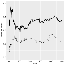
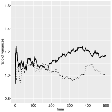
Figure 2: Estimation of the log-likelihood function as a function of $t$. The left (resp. right) plot gives the variance of SMC based on unordered stratified resampling divided by that of SMC based on Hilbert-ordered stratified resampling (resp. unordered SSP resampling). Continuous lines are for SMC based on the guided proposal while the dotted line is for the bootstrap particle filter. Results are based on 1 000 independent runs of the algorithms with $N=2^{13}$ particles.

6 Conclusion

Our results support the practice in the SMC literature to abandon multinomial resampling for stratified resampling by providing strong theoretical guarantees for this resampling scheme, which has the remarkable property to be both cheaper and more accurate than multinomial resampling. For the same reasons, our results should encourage practitioners to abandon residual resampling for a version of this residual method where the multinomial resampling step is replaced by a stratified resampling step.

The systematic resampling scheme fails to produce offspring numbers that are negatively associated. As an alternative to it we have introduced the SSP resampling algorithm which (1) is similar to systematic resampling in term of offspring numbers and (2) verifies the conditions of our general consistency result. We also built an example suggesting that any general consistency results for systematic resampling would require to take into account the order of the input particles and have established its validity when they are ordered along the Hilbert curve.

Our practical recommendation is to prefer SSP resampling to systematic resampling since both have similar properties while only the former has been proven to be consistent. Systematic resampling has the advantage to be faster than SSP resampling but in most cases this gain is likely to be imperceptible. Our simulation study suggests that SSP resampling outperforms also stratified resampling in term of variance but no theoretical result exists to support this observation.

We have also derived various results showing that the variance of stratified resampling goes to zero faster than $N^{-1}$ when applied on an input point set ordered along the Hilbert curve, and notably a non-asymptotic bound of size $N^{-1-\frac{1}{d}}$. Unsurprisingly, when the dimension of the state-space is small and/or when a good proposal distribution is available, our simulation results show that ordering the particle before applying stratified resampling may lead to important variance reduction. These theoretical results on the variance of Hilbert ordered stratified resamplig are also of particular interest for sequential quasi-Monte Carlo (Gerber and Chopin,, 2015), a quasi-Monte Carlo version of SMC, that converges at a faster but currently unknown rate.

Appendix A Convergent sequences of probability measures: star norm and transformations through the Hilbert curve and its inverse

The following theorem is the main tool for establishing Theorem 3.

Theorem 9.

Let $\mathcal{X}$ be a cubifiable set, $(\pi^{N})_{N\geq 1}$ be a sequence in $\mathcal{P}(\mathcal{X})$, $\pi\in\widetilde{\mathcal{P}}_{b}(\mathcal{X})$ and $\psi\in\mathcal{D}(\mathcal{X})$ be such that $\pi_{\psi}\in\mathcal{P}_{b}((0,1)^{d})$. Then, the following assertions are equivalent

1. $\pi^{N}\xRightarrow{\text{w}}\pi$;

2. $\lim_{N\rightarrow+\infty}\|\pi^{N}-\pi\|_{\star}=0$;

3. $\lim_{N\rightarrow+\infty}\|\pi_{h_{\mathcal{X},\psi}}^{N}-\pi_{h_{\mathcal{X},\psi}}\|_{\star}=0$;

4. $\pi_{h_{\mathcal{X},\psi}}^{N}\xRightarrow{\text{w}}\pi_{h_{\mathcal{X},\psi}}$.

Implications $(ii)\Rightarrow(iii)$ and $(iii)\Rightarrow(ii)$ respectively are due to Gerber and Chopin, (2015, Theorem 3) and Schretter et al., (2016, Theorem 1). Implications $(ii)\Rightarrow(i)$ and $(iii)\Rightarrow(iv)$ are direct applications of the Portmanteau lemma (e.g. van der Vaart,, 1998, Lemma 2.2, p.6). Implication $(i)\Rightarrow(ii)$ for $d=1$ holds by Polyà’s theorem (Pólya,, 1920; see also Bickel and Millar,, 1992, result (A.1)); note that Polyà’s theorem only requires that $\pi\in\mathcal{P}(\mathcal{X})$ is such that $F_{\pi}$ is continuous. Implication $(i)\Rightarrow(ii)$ for $d>1$ is new and proved following a similar argument as in Kuipers and Niederreiter, (1974, Theorem 1.2, p.89) while implication $(iv)\Rightarrow(iii)$ is a consequence of Polyà’s Theorem and of the continuity of $F_{\pi_{h_{\mathcal{X},\psi}}}$, which is established in the next lemma.

Lemma 2.

Let $\mathcal{X}$ be a cubifiable set, $\pi\in\widetilde{\mathcal{P}}_{b}(\mathcal{X})$ and $\psi\in\mathcal{D}(\mathcal{X})$ be such that $\pi_{\psi}\in\mathcal{P}_{b}((0,1)^{d})$. Then, $\pi_{h_{\mathcal{X},\psi}}$ is a continuous probability measure on $(0,1)$.

We also note the proofs of implications $(ii)\Rightarrow(iii)$ and $(iii)\Rightarrow(ii)$ in Gerber and Chopin, (2015, 2017); Schretter et al., (2016) implicitly assume that the sequence $(\pi^{N})_{N\geq 1}$ is such that (with $\mathcal{X}=(0,1)^{d}$)

$$\pi^{N}(\mathcal{H}_{d})=0,\quad\text{for all $N$ large enough}$$

where $\mathcal{H}_{d}$ is the set of points of $[0,1]^{d}$ that have more than pre-image through $H$. This point is corrected in the supplementary materials where a complete proof of Theorem 9 is provided.

See pages - of supplement.pdf

References

• Aistleitner and Dick, (2015) Aistleitner, C. and Dick, J. (2015). Functions of bounded variation, signed measures, and a general Koksma-Hlawja inequality. Acta Arith., 167(2):143–171.
• Andrieu et al., (2010) Andrieu, C., Doucet, A., and Holenstein, R. (2010). Particle Markov chain Monte Carlo methods. J. R. Stat. Soc. Ser. B Stat. Methodol., 72(3):269–342.
• Barbe and Bertail, (1995) Barbe, P. and Bertail, P. (1995). The weighted bootstrap, volume 98 of Lecture Notes in Statistics. Springer-Verlag, New York.
• Bertail et al., (2017) Bertail, P., Chautru, E., and Clémençon, S. (2017). Empirical processes in survey sampling with (conditional) poisson designs. Scand. J. Stat., 44(1):97–111.
• Bickel and Millar, (1992) Bickel, P. and Millar, P. (1992). Uniform convergence of probability measures on classes of functions. Statist. Sinica, pages 1–15.
• Cappé et al., (2005) Cappé, O., Moulines, E., and Rydén, T. (2005). Inference in hidden Markov models. Springer Series in Statistics. Springer, New York.
• Carpenter et al., (1999) Carpenter, J., Clifford, P., and Fearnhead, P. (1999). Improved particle filter for nonlinear problems. IEE Proc. Radar, Sonar Navigation, 146(1):2–7.
• Chopin, (2004) Chopin, N. (2004). Central limit theorem for sequential Monte Carlo methods and its application to Bayesian inference. Ann. Statist., 32(6):2385–2411.
• Cornebise et al., (2008) Cornebise, J., Moulines, É., and Olsson, J. (2008). Adaptive methods for sequential importance sampling with application to state space models. Stat. Comput., 18(4):461–480.
• Crisan, (2001) Crisan, D. (2001). Particles filters – a theoretical perspective. In Doucet, A., de Freitas, N., and Gordon, N. J., editors, Sequential Monte Carlo methods in practice, Stat. Eng. Inf. Sci., pages 17–41. Springer, New York.
• Crisan and Doucet, (2002) Crisan, D. and Doucet, A. (2002). A survey of convergence results on particle filtering methods for practitioners. IEEE Trans. Signal Process., 50(3):736–746.
• Del Moral and Doucet, (2003) Del Moral, P. and Doucet, A. (2003). On a class of genealogical and interacting Metropolis models. In Séminaire de Probabilités XXXVII, pages 415–446. Springer.
• Deville and Tille, (1998) Deville, J.-C. and Tille, Y. (1998). Unequal probability sampling without replacement through a splitting method. Biometrika, 85(1):89–101.
• Douc et al., (2005) Douc, R., Cappé, O., and Moulines, E. (2005). Comparison of resampling schemes for particle filtering. In ISPA 2005. Proceedings of the 4th International Symposium on Image and Signal Processing and Analysis, pages 64–69. IEEE.
• Douc et al., (2009) Douc, R., Moulines, E., and Olsson, J. (2009). Optimality of the auxiliary particle filter. Probab. Math. Statist., 29(1):1–28.
• Doucet et al., (2001) Doucet, A., de Freitas, N., and Gordon, N. J. (2001). Sequential Monte Carlo Methods in Practice. Springer-Verlag, New York.
• Dubhashi et al., (2007) Dubhashi, D., Jonasson, J., and Ranjan, D. (2007). Positive influence and negative dependence. Combin. Probab. Comput., 16(01):29–41.
• Dubhashi and Ranjan, (1998) Dubhashi, D. and Ranjan, D. (1998). Balls and bins: a study in negative dependence. Random Structures Algorithms, 13(2):99–124.
• Gerber and Chopin, (2015) Gerber, M. and Chopin, N. (2015). Sequential quasi Monte Carlo. J. R. Stat. Soc. Ser. B. Stat. Methodol., 77(3):509–579.
• Gerber and Chopin, (2017) Gerber, M. and Chopin, N. (2017). Convergence of sequential quasi-Monte Carlo smoothing algorithms. Bernoulli, 23(4B):2951–2987.
• Gordon et al., (1993) Gordon, N. J., Salmond, D. J., and Smith, A. F. M. (1993). Novel approach to nonlinear/non-Gaussian Bayesian state estimation. IEE Proc. F, Comm., Radar, Signal Proc., 140(2):107–113.
• Guarniero et al., (2017) Guarniero, P., Johansen, A. M., and Lee, A. (2017). The iterated auxiliary particle filter. J. Amer. Statist. Assoc., 112(520):1636–1647.
• He and Owen, (2016) He, Z. and Owen, A. B. (2016). Extensible grids: uniform sampling on a space filling curve. J. R. Stat. Soc. Ser. B. Stat. Methodol., 78(4):917–931.
• Jaffard and Nicolay, (2009) Jaffard, S. and Nicolay, S. (2009). Pointwise smoothness of space-filling functions. Appl. Comput. Harmon. Anal., 26(2):181–199.
• Joag-Dev and Proschan, (1983) Joag-Dev, K. and Proschan, F. (1983). Negative association of random variables with applications. Ann. Statist., 11(1):286–295.
• Johansen and Doucet, (2008) Johansen, A. M. and Doucet, A. (2008). A note on auxiliary particle filters. Statist. Probab. Lett., 78(12):1498–1504.
• Kitagawa, (1996) Kitagawa, G. (1996). Monte Carlo filter and smoother for non-gaussian state space models. J. Comput. Graph. Statist., 5(1):1–25.
• Kramer et al., (2011) Kramer, J. B., Cutler, J., and Radcliffe, A. J. (2011). Negative dependence and Srinivasan’s sampling process. Combin. Probab. Comput., 20(03):347–361.
• Kuipers and Niederreiter, (1974) Kuipers, L. and Niederreiter, H. (1974). Uniform distribution of sequences. Wiley-Interscience.
• Künsch, (2005) Künsch, H. R. (2005). Recursive Monte Carlo filters: algorithms and theoretical analysis. Ann. Statist., 33(5):1983–2021.
• L’Ecuyer and Lemieux, (2000) L’Ecuyer, P. and Lemieux, C. (2000). Variance reduction via lattice rules. Management Science, 46(9):1214–1235.
• Liu and Chen, (1998) Liu, J. S. and Chen, R. (1998). Sequential Monte Carlo methods for dynamic systems. J. Amer. Statist. Assoc., 93(443):1032–1044.
• Madow and Madow, (1944) Madow, W. G. and Madow, L. H. (1944). On the theory of systematic sampling, i. The Annals of Mathematical Statistics, 15(1):1–24.
• Niederreiter, (1992) Niederreiter, H. (1992). Random number generation and quasi-Monte Carlo methods, volume 63 of CBMS-NSF Regional Conference Series in Applied Mathematics. Society for Industrial and Applied Mathematics (SIAM), Philadelphia, PA.
• Pitt and Shephard, (1999) Pitt, M. K. and Shephard, N. (1999). Filtering via simulation: auxiliary particle filters. J. Amer. Statist. Assoc., 94(446):590–599.
• Pólya, (1920) Pólya, G. (1920). Über den zentralen grenzwertsatz der wahrscheinlichkeitsrechnung und das momentenproblem. Mathematische Zeitschrift, 8(3):171–181.
• Schretter et al., (2016) Schretter, C., He, Z., Gerber, M., Chopin, N., and Niederreiter, H. (2016). Van der Corput and golden ratio sequences along the Hilbert space-filling curve. In Monte Carlo and Quasi-Monte Carlo Methods, pages 531–544. Springer.
• Shao, (2000) Shao, Q.-M. (2000). A comparison theorem on moment inequalities between negatively associated and independent random variables. J. Theoret. Probab., 13(2):343–356.
• Srinivasan, (2001) Srinivasan, A. (2001). Distributions on level-sets with applications to approximation algorithms. In Foundations of Computer Science, 2001. Proceedings. 42nd IEEE Symposium on, pages 588–597. IEEE.
• Stein, (1987) Stein, M. (1987). Large sample properties of simulations using Latin hypercube sampling. Technometrics, 29(2):143–151.
• Tillé, (2006) Tillé, Y. (2006). Sampling algorithms. Springer Series in Statistics. Springer, New York.
• van der Vaart, (1998) van der Vaart, A. W. (1998). Asymptotic statistics, volume 3 of Cambridge Series in Statistical and Probabilistic Mathematics. Cambridge University Press, Cambridge.
• Zumbusch, (2003) Zumbusch, G. (2003). Parallel multilevel methods. Springer.