Quench dynamics in superconducting nanojunctions: metastability and dynamical Yang-Lee zeros

Abstract

We study the charge transfer dynamics following the formation of a phase or voltage biased superconducting nano-junction using a full counting statistics analysis. We demonstrate that the evolution of the zeros of the generating function allows one to identify the population of different many body states much in the same way as the accumulation of Yang-Lee zeros of the partition function in equilibrium statistical mechanics is connected to phase transitions. We give an exact expression connecting the dynamical zeros to the charge transfer cumulants and discuss when an approximation based on “dominant” zeros is valid. We show that, for generic values of the parameters, the system gets trapped into a metastable state characterized by a non-equilibrium population of the many body states which is dependent on the initial conditions. We study in particular the effect of the switching rates in the dynamics showing that, in contrast to intuition, the deviation from thermal equilibrium increases for the slower rates. In the voltage biased case the steady state is reached independently of the initial conditions. Our method allows us to obtain accurate results for the steady state current and noise in quantitative agreement with steady state methods developed to describe the multiple Andreev reflections regime. Finally, we discuss the system dynamics after a sudden voltage drop showing the possibility of tuning the many body states population by an appropriate choice of the initial voltage, providing a feasible experimental way to access the quench dynamics and control the state of the system.

I Introduction

The physics of superconducting devices is receiving a renewed attention in parallel with ongoing proposals of applications in quantum technologies Devoret and Schoelkopf (2013). While most common designs are based on conventional tunnel junctions, proposals based on hybrid nanostructures like those being explored in the search of Majorana bound states are generating a great research activity Alicea (2012); Beenakker (2015).

In these devices a challenging issue is to avoid decoherence for certain low energy states while at the same time being able to manipulate them coherently by means of external fields Plugge et al. (2017). An important source of decoherence arises from quasiparticle tunneling Martinis et al. (2009); Catelani et al. (2011); Ristè et al. (2013); Avriller and Pistolesi (2015). The so-called quasiparticle “poisoning” can become an obstacle towards the implementation of Majorana qubits Rainis and Loss (2012); Colbert and Lee (2014); Bespalov et al. (2016); Albrecht et al. (2017). Conversely, long lived states arising from trapped quasiparticles in Andreev bound states (ABS) Zgirski et al. (2011); Olivares et al. (2014) have been suggested as possible realizations of a spin qubit Padurariu and Nazarov (2012).

Superconducting nanodevices are also of fundamental interest as an example of an interacting open quantum system, which can be driven out of equilibrium by different means and can exhibit highly non-trivial dynamical behavior Nazarov and Yaroslav (2009). While the theory has traditionally focused on the stationary transport properties, advances in single electron sources and detection techniques are allowing to explore the response of nanodevices in the time domain over increasingly smaller time scales Fève et al. (2007); Bocquillon et al. (2013); Dubois et al. (2013). Moreover, it is becoming clear that the dynamics of open quantum systems can exhibit singular features which are not necessarily reflected in their stationary properties Garrahan and Lesanovsky (2010); Heyl et al. (2013); Karrasch and Schuricht (2013). These features can be revealed from the full counting statistics (FCS) analysis of time-integrated observables Hickey et al. (2013a). The analogy between equilibrium statistical mechanics and FCS methods suggests that the behavior of the zeros of the generating function in FCS theory could allow to identify dynamical transitions much in the same way as the Yang-Lee zeros Yang and Lee (1952); Lee and Yang (1952) of the partition function are connected to phase transitions in the static case Utsumi et al. (2013); Peng et al. (2015); Ivanov and Abanov (2013).

In a recent work we have presented a FCS analysis of the quench dynamics in the formation of a superconducting nanojuction Souto et al. (2016). We showed that, under rather general conditions, many body states with different parity get a significant population and that their relaxation towards thermal equilibrium requires the interaction with external degrees of freedom. In the present work we discuss the phenomenon from the broader perspective which is provided by analyzing the dynamics of the FCS Yang-Lee zeros. In contrast to previous works in this direction Flindt and Garrahan (2013); Hickey et al. (2014); Brandner et al. (2017); Flindt et al. (2009), we consider the system evolution at time scales shorter than the typical Markovian times Zgirski et al. (2011). We study the connection between the structure of the dynamical Yang-Lee zeros (DYLZ) in the complex plane and the formation of metastable many body states. Moreover, we show that by tuning a counting parameter, the current cumulants tend to exhibit a singular behavior which is reminiscent of the divergences of correlation functions in a first order phase transition.

The paper is organized as follows: In Sec. II we introduce the model used for describing the dynamics of a nanoscale normal region coupled to superconducting leads and discuss the FCS formalism. We pay particular attention to the definition of the DYLZ within this context and their connection to the current cumulants. In Sec. III we explore in detail the transient dynamics in quantities like the mean charge and current. The influence of the initial conditions in the formation of ABSs and their effect in the system charge and current evolution is also analyzed, showing that it decreases with an increasing coupling to the leads. We also explore in this section the effect of the switching rate in the contact formation. Sec. IV is devoted to the FCS analysis of the quench dynamics. We show how FCS predicts an evolution from a Poissonian distribution at short times into a three-modal distribution at larger times which can be associated to the formation of three different many body states. We discuss how a coarse grained representation can be defined and how the population of the many body states can be extracted from it. We then give the analysis of the evolution of the DYLZ showing how the different many body states can be identified from their accumulation in the complex plane. It is also shown that the scaling of the current cumulants at large times can be extracted from the dominant DYLZ. The analysis is then extended to the case of voltage biased junctions (Sec. V), discussing how the steady state is reached for quantities such as current and noise. This is also illustrated from the evolution of the subgap spectral densities. Furthermore, we study the FCS and analyze the particular accumulation of DYLZ for this voltage biased case. Finally, in Sec. VI we analyze the case of a different initialization procedure consisting in a dc voltage switch off, demonstrating the possibility of controlling the population of the different many body states by a proper selection of the applied bias. Sec. VII is devoted to some concluding remarks.

II Model and formalism

Our model consists of a central region represented by a spin-degenerate quantum level, coupled to two BCS superconducting electrodes. Low energy electron transport in this kind of structure is dominated by multiple Andreev reflections, leading to the formation of subgap states, located at $\pm\epsilon_{A}$ in the zero bias limit. The aim of the present work is the analysis of the transient transport properties through the system after a sudden connection at $t=0$ of the central region to the electrodes, which could be phase or voltage biased.

The system Hamiltonian, $H=H_{leads}+H_{0}+H_{T}$, can be written in terms of Nambu spinors $\hat{\Psi}^{\dagger}_{j}=\left(c^{\dagger}_{j\uparrow},c_{j\downarrow}\right)$, where $j=k\nu,0$ denotes the $\nu=L,R$ lead and the central level states respectively. The uncoupled Hamiltonians are given by $H_{0}=\hat{\Psi}^{\dagger}_{0}\hat{h}_{0}\hat{\Psi}_{0}$, $H_{leads}=\sum_{k\nu}\hat{\Psi}^{\dagger}_{k\nu}\hat{h}_{k\nu}\hat{\Psi}_{k\nu}$, while the tunneling term is $H_{T}=\sum_{k,\nu}\left[\hat{\Psi}^{\dagger}_{k\nu}\hat{V}_{\nu}(t)\hat{\Psi}_{0}+\mbox{h.c.}\right]$, where $\hat{h}_{0}=\epsilon_{0}\sigma_{z}$ and $\hat{h}_{k\nu}=\epsilon_{k\nu}\sigma_{z}+\Delta_{\nu}\sigma_{x}$ ($\sigma_{z}$ and $\sigma_{x}$ denote here Pauli matrices in the Nambu space). The superconducting gap parameter will be taken equal for both electrodes, $\Delta_{L}=\Delta_{R}\equiv\Delta$, and used as the energy unit. For describing the connection between the system and the electrodes we use $\hat{V}_{\nu}(t)=f(t)V^{0}_{\nu}\sigma_{z}e^{i\sigma_{z}\phi_{\nu}(t)/2}$, where $f(t)$ is a function controlling the abruptness of the connection as discussed below and $\phi_{L}(t)-\phi_{R}(t)=\phi(t)$ determines the phase difference between the leads.

For simplicity we consider a constant normal density of states $\rho_{L,R}$ in the leads with a finite bandwidth $W$ taken as the largest energy scale in the model. We define the stationary tunneling rates as $\Gamma_{\nu}=\pi(V^{0}_{\nu})^{2}\rho_{\nu}$, and $\Gamma=\Gamma_{L}+\Gamma_{R}$. For later use, we also define the normal transmission coefficient as $\tau=4\Gamma_{L}\Gamma_{R}/(\Gamma^{2}+\epsilon_{0}^{2})$. Depending on the relative value between the tunneling rates and the superconducting gap, two regimes can be identified: the quantum dot (QD) regime, corresponding to $\Gamma\lesssim\Delta$ and the quantum point contact (QPC) regime, where $\Gamma\gg\Delta$. Finally, the central level initial charge will be denoted by $n_{\sigma}(0)$, where $\sigma\equiv\uparrow,\downarrow$. Hereafter we assume $\hbar=e=1$.

The time-dependent transport properties of the system are fully characterized by the generating function (GF) defined on the Keldysh contour as Levitov (2002)

$$Z(\chi,t)=\left\langle T_{K}exp\left[-i\int_{C}dt^{\prime}H_{T,\chi}(t^{\prime})\right]\right\rangle_{0},$$ (1)

where $T_{K}$ is the contour time order operator, $\chi\equiv\chi_{\nu}(t)$ are counting fields entering as phase factors modulating the hopping terms in $H_{T}$, having opposite values $\pm\chi_{\nu}$ on the two branches of the Keldysh contour. The average in Eq. (1) is taken over the decoupled system. The GF gives access to the charge transfer cumulants, i.e. $C^{n}(t)=(i)^{n}\partial^{n}\mathcal{S}/\partial\chi^{n}\rfloor_{0}$, where $\mathcal{S}(\chi,t)=\ln Z(\chi,t)$. The charge cumulants through the left (right) electrodes can be computed by imposing $\chi_{L}=\chi$ and $\chi_{R}=0$ ($\chi_{L}=0$ and $\chi_{R}=-\chi$), and for the symmetrized charge cumulants $\chi_{L}=\chi/2$ and $\chi_{R}=-\chi/2$. The corresponding current cumulants are given by $I^{n}(t)=\partial C^{n}/\partial t$. The symmetrized cumulants will be denoted $\left\langle I^{n}\right\rangle$, using $\left\langle S\right\rangle=\left\langle I^{2}\right\rangle$ for the symmetrized shot noise. As shown in Cohen et al. (2014); Chen et al. (2016), the occupied Density Of States (DOS) in the transient regime can be computed from the current to an empty normal electrode, weakly coupled to the central region.

It can be shown that $Z(\chi,t)$ can be computed as a Fredholm determinant on the Keldysh contour Kamenev (2011); Esposito et al. (2009); Tang et al. (2014); Tang and Wang (2014); Seoane Souto et al. (2015). A straightforward extension of this formalism to the superconducting case Souto et al. (2016) leads to

$$Z(\chi,t)=\mbox{det}\left[{\bf G}(\chi=0){\bf G}(\chi)^{-1}\right],$$ (2)

where ${\bf G}=-i\left\langle T_{K}\Psi_{0}(t)\Psi_{0}^{\dagger}(t^{\prime})\right\rangle$ is the Green function of the dot coupled to the leads defined in Keldysh-Nambu space. Using the Dyson equation, Eq. (2) can be written as

$$Z(\chi,t)=\det\left[{\bf G}\left({\bf g}_{0}^{-1}-\tilde{\bf\Sigma}\right)\right]\;,$$ (3)

where ${\bf g}_{0}$ denotes the uncoupled central level Green function and $\tilde{\bf\Sigma}=\tilde{\bf\Sigma}_{L}+\tilde{\bf\Sigma}_{R}$ corresponds to the leads self-energy in which the counting field $\chi$ is included. The Keldysh-Nambu components of the self-energy are given by

$$\tilde{\Sigma}^{\alpha\beta}_{\nu,jk}(t,t^{\prime})=f(t)f(t^{\prime})s_{\alpha}s_{\beta}s_{j}s_{k}\left(V^{0}_{\nu}\right)^{2}e^{i(s_{j}-s_{k})\phi_{\nu}/2}$$

$$e^{i(s_{\alpha}s_{j}-s_{\beta}s_{k})\chi_{\nu}/2}g^{\alpha\beta}_{jk}(t-t^{\prime}),$$ (4)

where $\alpha\beta\equiv\pm$ are the Keldysh indexes, $j\,k\equiv\pm$ are the Nambu ones, $\nu=L,R$ denote the leads, $s_{\pm}=\pm 1$, $s_{j}=(-1)^{(j+1)}$ and $g^{\alpha\beta}_{jk}(t-t^{\prime})$ are the uncoupled leads Green functions. Eq. (2) has to be integrated numerically by discretizing the Keldsyh contour as depicted in Fig. 1 (for details see Supplemental Material in Ref. Souto et al. (2016)). Analytical results, which can be obtained in certain limits, will allow us to further clarify our findings as described below.

On the other hand, the GF can be decomposed as

$$Z(\chi,t)=\sum_{n}P_{n}(t)e^{i\chi n}\;,$$ (5)

where $P_{n}(t)$ can be associated with the probability of transferring $n$ charges in the measuring time $t$ Nazarov and Yaroslav (2009). In the superconducting case, the charge in the leads is not well defined, and $P_{n}(t)$ can eventually take negative values Belzig and Nazarov (2001); Shelankov and Rammer (2003); Hofer and Clerk (2016). The $P_{n}(t)$ are therefore referred to in this case as quasi-probabilities.

Figure 1: Keldysh contour considered to analyze the transient regime. $\chi$ indicates the counting field changing sign on the two branches of the contour and $\delta t$ corresponds to the time step in the discretized calculation of the dot Green function and the generating function $Z(\chi,t)$.

II.1 Relation between DYLZs and cumulants

In their seminal papers, T. D. Lee and C. N. Yang demonstrated the connection between thermodynamical phase transitions and the behavior of the roots of the partition function Yang and Lee (1952); Lee and Yang (1952). They discussed how these roots accumulate to form branches in the complex plane of a given variable, $z$, dependent on the system’s temperature. The phase diagram of the system is determined by the interceptions of these branches with the positive real axis in the thermodynamical limit (i.e. as the volume tends to infinity). The crossing points correspond to situations where two (or more phases) coexist. These ideas, originally developed for equilibrium statistical mechanics, have recently been applied to the study of the time evolution of open quantum systems Hickey et al. (2013b); Brandner et al. (2017), with the time playing the extensive role of the volume, the GF of Eq. (5) the role of the partition function and $z\equiv e^{i\chi}$. By analogy, the roots of the GF in the complex $z$ plane are referred to as Dynamical Yang-Lee Zeros (DYLZs). The position of the DYLZs, denoted by $z_{j}(t)$, fully characterize the transport properties through the system, and Eq. (5) can be rewritten as

$$Z(z,t)=\prod_{j}(z-z_{j}(t))\;.$$ (6)

In a previous work we derived exact expressions for the charge cumulants of arbitrary order Seoane Souto et al. (2017). In terms of the DYLZs these can be written as

$$C^{n}(t)=-\sum_{j}\mbox{Li}_{1-n}\left(\frac{1}{z_{j}(t)}\right)$$ (7)

where Li_j denotes the polylogarithm function of order $j$ Abramowitz and Stegun (1964). The main contribution to the charge cumulants is provided by the DYLZs close to $z=1$, where the functions diverge. For the higher order cumulants, the exact expression Eq. (7) can be well approximated by Berry (2005); Flindt et al. (2010); Kambly et al. (2011)

$$C^{n}(t)\approx(-1)^{n-1}(n-1)!\sum_{j}\frac{2\cos\left\{n\,\mbox{arg}\left[z_{j}(t)-1\right]\right\}}{\left|z_{j}(t)-1\right|^{n}}\,.$$ (8)

Additional information can be obtained from the so-called factorial cumulants, which are a generalization of the conventional ones, defined by shifting the measurement point in the z-plane. These quantities provide valuable information about the interactions in mesoscopic systems Kambly et al. (2011); Stegmann et al. (2015); Stegmann and König (2016). The factorial generating function (FGF) can be written as

$$Z_{F}(z,t;s)=\frac{\sum_{n}P_{n}\left(z+s\right)^{n}}{\sum_{n}s^{n}P_{n}}\;,$$ (9)

where $s$ is a biasing field. Notice that the denominator is a normalization factor and does not contribute to the transport properties, since it does not depend on the counting field. One can also define the DYLZs of the FGF, which are just the original $z_{j}(t)$ shifted by $s$. Thus, the factorial cumulants are given by

$$C^{n}_{F}(t;s)=-\sum_{j}\mbox{Li}_{1-n}\left[\frac{1}{z_{j}(t)+s}\right]\;,$$ (10)

The current cumulants ($I^{n}$) and the factorial current cumulants ($I^{n}_{F}$) can be then computed by deriving Eqs. (7) and (10) with respect to time, respectively. Again we shall define $\left\langle I^{2}_{F}\right\rangle=\left\langle S_{F}\right\rangle$ for the symmetrized factorial shot noise.

III Transient dynamics

In this section we analyze the time evolution of single particle observables (charge, current and spectral densities) after a sudden switch on of the central level-leads coupling for the phase biased case. Parameters are chosen in order to study the different behavior from the QD to the QPC regimes. Unless stated differently, we consider in this section the electron hole-symmetric case $\epsilon_{0}=0$ and $\Gamma_{L}=\Gamma_{R}$. This choice corresponds to a case of perfect transmission where the nonequilibrium effects that we are interested in are more pronounced.

III.1 Central level charge evolution and ABSs formation

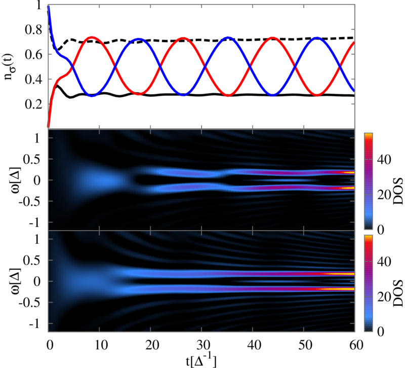
Figure 2: Top panel: Time evolution of the central level population for three different initial configurations: $(n_{\uparrow}(0),n_{\downarrow}(0))=(0,0)$ (red line), $(1,1)$ (blue line), where $n_{\uparrow}(t)=n_{\downarrow}(t)$, and $(0,1)$ (black line, using solid line for $n_{\uparrow}(t)$, and the dashed one for $n_{\downarrow}(t)$). Lower panels: time evolution of the occupied density of states (DOS) for the (0,0) and (0,1) initial configurations. We consider a perfect transmitting junction in the quantum dot regime with $\Gamma=0.5$ (in units of $\Delta$) and $\phi=2$.

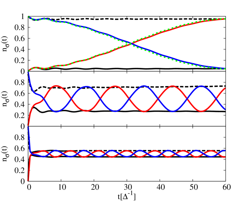
Figure 3: Time evolution of the level population for three different initial configurations: $(n_{\uparrow}(0),n_{\downarrow}(0))=(0,0)$ (red line), $(1,1)$ (blue line) and $(0,1)$ (black line, using solid line for the population of spin up electrons, and the dashed one for spin down). The dotted line in the upper panel shows the comparison to the approximation described in the appendix A. We show the evolution of the behavior of the population for three different couplings between the central level and the electrodes $\Gamma=0.05$, $0.5$ and $2$, from top to bottom, for a phase difference $\phi=2$.

In Fig. 2 we show results for the charge per spin and the subgap occupied spectral density evolution after a sudden connection, i.e. $f(t)=\theta(t)$, for three different initial configurations, $(n_{\uparrow}(0),n_{\downarrow}(0))=(0,0),(1,1)$ and $(0,1)$ and $\Gamma=\Delta/2$. At short times, $t\lesssim 1/\Delta$, the initial excess charge tends to relax through the electrodes. A change in this tendency is observed at times of the order $t\sim 2/\Delta$ coinciding with the incipient formation of the ABSs inside the gap which block the excess charge relaxation. While for the initial configurations $(0,1)$ or $(1,0)$ the system gets trapped in a metastable magnetic state, with $n_{\uparrow}\neq n_{\downarrow}$, for the initial configurations $(0,0)$ and $(1,1)$ the charge oscillates but the system remains non-magnetic. The period of the oscillation is $\sim\pi/|\epsilon_{A}|$, where $\epsilon_{A}\simeq\Gamma\cos(\phi/2)$ corresponds to the ABS energy in the QD regime. It should be also noticed that the oscillations corresponding to the $(0,0)$ and the $(1,1)$ configurations are displaced in half a period. Remarkably, as we show in the next subsection, in all these cases the system exhibits the same symmetrized current.

As shown in Ref. Souto et al. (2016), one can get an analytical insight on this behavior as the spectral weight in this QD regime is mainly concentrated on the ABSs and the retarded dot Green function can be approximated by just the contribution from these states. In Ref. Souto et al. (2016) we analyzed the charge evolution starting from the initial magnetic configuration $(0,1)$. The corresponding analysis for an arbitrary initial configuration is given in Appendix A. As we show in this Appendix the dot charge oscillations for the $(0,0)$ case can be approximated as $2|P_{12}|^{2}[1-\cos(2\epsilon_{A}t)]$, where

$$|P_{12}|^{2}=\frac{\left(1-\Gamma/\Delta\right)^{2}-\epsilon_{0}^{2}/\epsilon_{A}^{2}}{4\left(1+\epsilon_{A}^{2}/\Delta^{2}\right)}\,.$$ (11)

These oscillations remain undamped unless an additional relaxation mechanism is included. The amplitude is determined by the coupling between the two ABSs ($P_{12}$), generated by the initial conditions. This behavior is also reflected in the occupied DOS, shown in the middle panel of Fig. 2 for the $(0,0)$ initial condition. We show that the dot’s charge oscillations are correlated with an intermittent behavior of the population of the ABSs. This behavior is absent in the half-filled initial condition (lower panel in Fig. 2).

In Fig. 3 we show the charge evolution for the same initial configurations studied in Fig. 2 for three different couplings to the electrodes, $\Gamma=0.05$, $0.5$ and $2$ (in units of $\Delta$), from top to bottom. As commented before in the QD regime, $\Gamma\lesssim\Delta$, for initially trapped quasi-particles (i.e. $(0,0)$ and $(1,1)$ configurations), the population exhibits large oscillations. The amplitude of these oscillations is monotonously reduced when increasing the hybridization, $\Gamma$. In the QPC regime, $\Gamma\gg\Delta$, the initial condition is almost fully relaxed at very short times ($t\sim 1/\Gamma)$ and the population tends to reach the expected stationary value $n_{\sigma}\sim 0.5$. However, as shown in Ref Souto et al. (2016), this relaxation of the initial excess charge does not imply a full thermalization of the system. This would be further analyzed in Sec. IV.

III.2 Current evolution

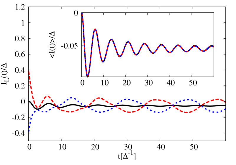
Figure 4: Left current evolution for three different initial configurations $(n_{\uparrow}(0),n_{\downarrow}(0))=(0,0)$ (dashed red line), $(1,1)$ (dotted blue line) and $(0,1)$ (solid black line). The parameters are the same as in Fig. 2. In the inset we show the independence on the initial conditions of the symmetrized current.

In this subsection we analyze the main results for the transient current flowing through the system after a sudden contact formation. In the main panel of Fig. 4 we show the current evolution at the left interface for the three initial configurations studied before. For the case with an initially trapped quasiparticle (blue and red curves), this current exhibits similar oscillations as found in the charge evolution, while for the $(0,1)$ case it approaches the mean value of the previous two cases (solid black like). On the other hand, the transient current becomes independent on the initial charge configuration when it is left-right symmetrized, as shown in the inset of Fig. 4. This fact demonstrates that most of the oscillatory behavior arises from the symmetric transfer of quasiparticles between the central region and the electrodes, which cancel out when the current is symmetrized. From now on we will focus on the properties of the symmetrized current.

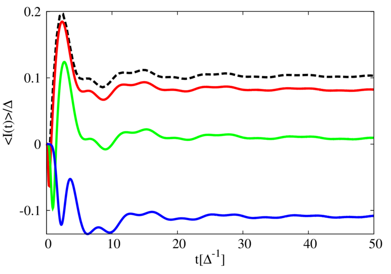
Figure 5: Transient current as a function of the switching rate $\alpha$ of the coupling between the electrodes and the central region (see text) for the case $\Gamma_{L}=\Gamma_{R}=5$. The dashed black curve shows the quench evolution, compared with three different connection rates, $\alpha=5$, $1$ and $0.25$, from top to bottom. The rest of parameters are the same as Fig. 2.

Another characteristic of the current flowing through the system is that the long-time asymptotic value does not reach the expected limit for a thermal equilibrium situation. The characterization of this metastable state has already been done in Ref. Souto et al. (2016) for a sudden quench of the coupling to the electrodes. An issue not addressed in that work was the effect of a decreasing switching rate. In Fig. 5 we show the current evolution in the point contact limit ($\Gamma\gg\Delta$) assuming $f(t)=\theta(t)[1-\exp(-\alpha t)]$, $\alpha$ being the connection rate. For a sufficiently fast connection, we recover the results of Ref. Souto et al. (2016) (dashed black curve). Surprisingly, for slower connection rates, the system gets trapped in a metastable state which deviates more strongly from the equilibrium situation, with a supercurrent which is even inverted for the smaller connection rates. This indicates that the trapping of the system in a metastable state is not an artifact of the abrupt connection, but is a rather general result. The behavior is better understood from the discussion of the Andreev states population in the next section.

III.3 Andreev states population

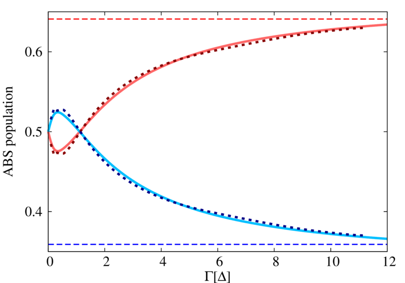
Figure 6: Occupation of the lower (red) and upper (blue) ABSs for the perfect transmitting case ($\epsilon=0$ and $\Gamma_{L}=\Gamma_{R}=\Gamma/2$) and $\phi=2$ as a function of $\Gamma$. The dashed lines show the asymptotic value in the point contact regime, given in Appendix B. The dotted line represents the long time population varying the connection rate $\alpha$, as a function of the effective tunneling rate $\Gamma_{eff}=\Gamma(1-(1-exp(-\alpha t_{A}))/\alpha t_{A})$, with $t_{A}=\sqrt{2}/\Delta$ and $\Gamma=12$.

A property that can be accessed from the transient current behavior is the population of the two ABSs. Using the symmetrized current and the fact that, in average, the two ABSs have to be half-filled, their population can be extracted. The set of equations used to extract the population are

$$\left\langle I\right\rangle = (n_{d}-n_{u})I_{A}+I_{c}$$

$$1 = n_{d}+n_{u}\;,$$ (12)

$n_{u}$ and $n_{d}$ being the population of the upper and lower ABS respectively, $I_{A}$ the equilibrium supercurrent supported by the lower ABS and $I_{c}$ the contribution from the continuum to the current. The long time average occupation of the two ABSs after a quench of the central region-leads coupling is shown in Fig. 6. For $\Gamma\ll\Delta$, the upper ABS is more populated than the lower one, leading to a current flowing in the opposite direction than the expected stationary value. This behavior is inverted at $\Gamma\sim\Delta$, as predicted by the analytical insight described in Appendix A. For $\Gamma\gg\Delta$ the system reaches a universal behavior, represented by the discontinuous lines. This universal behavior can be extracted from simple rate equations, assuming transition rates of the order of the distance between the continuum and the final states (see Appendix B).

Finally, the dotted lines in Fig. 6 show the Andreev states population for the smoother connection case, with an effective tunneling rate, $\Gamma_{eff}$, dependent on the connection rate $\alpha$. We observe similar features to the sudden quench situation, indicating that the quasiparticle relaxation happens at very short times (before the ABSs formation). After that initial stage, the two ABSs move adiabatically to their long time stationary value without exchanging charge.

IV Full Counting Statistics and Dynamical Yang-Lee Zeros

IV.1 Full counting statistics

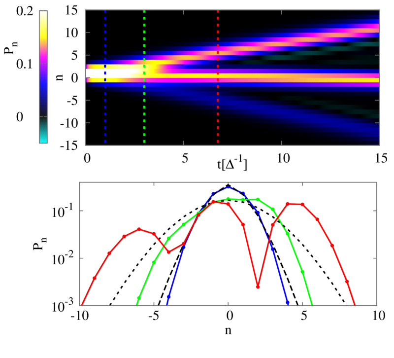
Figure 7: Upper panel: Time evolution of the quasiprobabilities, exhibiting the formation of three different states. In the lower panel we show some cuts at different times $t=1$ (blue) , $3$ (green) and $6$ (red). At short times, the probabilities can be interpreted as a birth-death distribution (discontinuous line) with equal birth and death rates (see appendix C for details). At times of the order of the creation of the ABSs, the distribution tends to deviate from the simple bidirectional poissonian distribution (comparing green curve to dotted one). At longer times (red curve), three states are created, related to the many body representation of the population of the ABSs.

In the QPC regime and for steady state conditions, the quantum state of the system can be characterized through the many body spectrum representation, corresponding to the four possible occupations of the ABSs Zgirski et al. (2011); Zazunov et al. (2014). In the ground state ($-$) only the lower ABS is occupied. An excited state of the same parity corresponds to populate only the upper ABS ($+$). Finally, there are two degenerate excitations involving a change in the parity of the system state, which will be referred to as odd states ($odd$), corresponding to populate or depopulate both ABSs simultaneously. While this simplified description does not hold at short times ($t<1/\epsilon_{A}$) in the transient regime, as it was shown in Ref. Souto et al. (2016), the population of these states can be inferred by analyzing the evolution of the asymptotic quasiprobabilities.

The upper panel of Fig. 7 shows the time evolution of the quasiprobabilities at short times, which evolve from a uni-modal distribution to a tri-modal one, related to the three states described above. In the lower panel of Fig. 7 we show some cuts before (blue) and just after this transition (red). At very short times (blue curve) the charge transfer is a random process that involves charge flowing in both directions, with similar probabilities. This short time dynamics can be described as a bidirectional Poisson distribution (see appendix C), shown as discontinuous lines in the lower panel of Fig. 7. The green line shows the probability distribution at the typical formation time of the ABSs. At this time, the probability distribution becomes asymmetric exhibiting a net charge flowing through the junction which deviates from the fitted bidirectional Poisson distribution (dotted curve). This fit provides an estimated number of $\sim 3$ electrons crossing the junction in each direction to create the subgap states. At longer times, the distribution exhibits three maxima, indicating the coexistence between the different many body states, which in the following will be referred to as (quantum) phases, in analogy with equilibrium statistical mechanics.

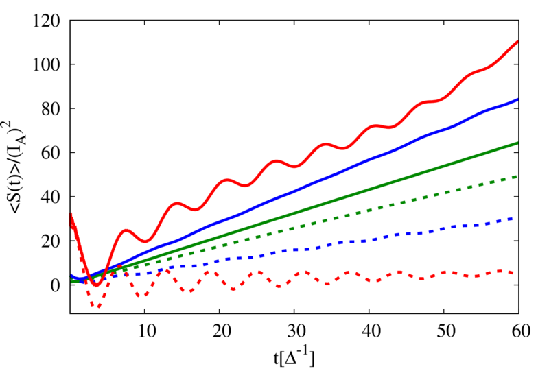
Figure 8: Symmetrized shot noise of the transferred charges for different initial conditions $(n_{\uparrow}(0),n_{\downarrow}(0))=(0,0)$ or $(1,1)$ (continuous lines) and $(1,0)$ (dashed lines) for three different dot electrodes coupling, $\Gamma=0.05$ (red), $0.5$ (blue) and $2$ (green) showing the sensitivity of the symmetrized noise to the initial conditions

Further insight on the system short time dynamics can be obtained by analyzing the current noise. In Fig. 8 we show some results for the symmetrized current noise for different couplings to the electrodes and initial configurations. As can be observed, differently from the symmetrized transient current or the ABS population, Eq. (12), the symmetrized noise is sensitive to the initial conditions. This fact shows that the actual many body state cannot be inferred solely from mean single particle properties, but requires the knowledge of higher order current cumulants. The dashed lines correspond to the evolution for an initial condition $(0,1)$, while the solid ones correspond to the evolution for initially trapped quasiparticles (cases $(0,0)$ and $(1,1)$). In all situations, we observe a linear increase of the noise with time, which can be considered as a signature of the phase coexistence. The noise becomes larger for the case of initially trapped quasi-particles, coinciding with the oscillations observed in the dot population. The dependence on the initial conditions decreases for increasing $\Gamma$. This dependence on the initial conditions is present also in the many body population of the ABSs, which fully characterize the state of the system.

IV.2 Coarse grained statistics

At long times a simplified coarse grained representation of the FCS can be introduced, where we approximate the probability map as three maxima disregarding their width. Their weights ($P_{-}$, $P_{+}$ and $P_{odd}$) can be computed by integrating the quasiprobabilities around their maxima. The three peaks evolve with time as $I_{\mu}t$ ($\mu=-,+,odd$) with

$$I_{-}=-I_{+}=I_{A}+I_{c}\quad\mbox{and}\quad I_{odd}=I_{c}\;.$$ (13)

This representation provides an accurate description of the transport properties in the long time regime, where the width of the three probability peaks becomes negligible compared to their separation. The long time GF can then be written as

$$Z(\chi)\approx P_{-}e^{i\chi I_{-}\,t}+P_{+}e^{i\chi I_{+}\,t}+P_{odd}e^{i\chi I_{odd}\,t}.$$ (14)

From this expression, the asymptotic position of the DYLZs can be obtained as

$$\alpha_{\pm}=z^{I_{A}t}_{\pm}\approx\frac{-P_{odd}\pm\sqrt{P_{odd}-4P_{-}P_{+}}}{2P_{-}}\,,$$ (15)

which corresponds to two branches, converging to the unitary circle centered in the coordinate’s origin. In the thermodynamical limit, a similar shape has already been reported in Ref. Lee and Yang (1952) for the Ising model, which describes the system undergoing a phase transition at $z=1$. The point $z=0$ is also a root of the GF with a degeneracy of $I_{+}t$. Using Eq. (7), simple expressions can be derived for the current cumulants, i.e.

$$\left\langle I^{n}\right\rangle\approx n\,I_{A}^{n}\,t^{n-1}\sum_{\pm}\mbox{Li}_{1-n}\left(\frac{1}{\alpha_{\pm}}\right)\,,$$ (16)

which describe the way the cumulants diverge with time. For instance, this equation characterizes the linear increase in the noise shown in Fig. 8. As it was pointed out in Ref. Souto et al. (2016), the long time current and noise (together with the normalization condition) provide a complete set of equations for determining the population of each of the three phases. Extrapolating this reasoning to the case of $p$ coexistent phases, the population of each of the phases could be determined by measuring the long time behavior of the first $p-1$ cumulants.

IV.3 Dynamical Yang-Lee zeros

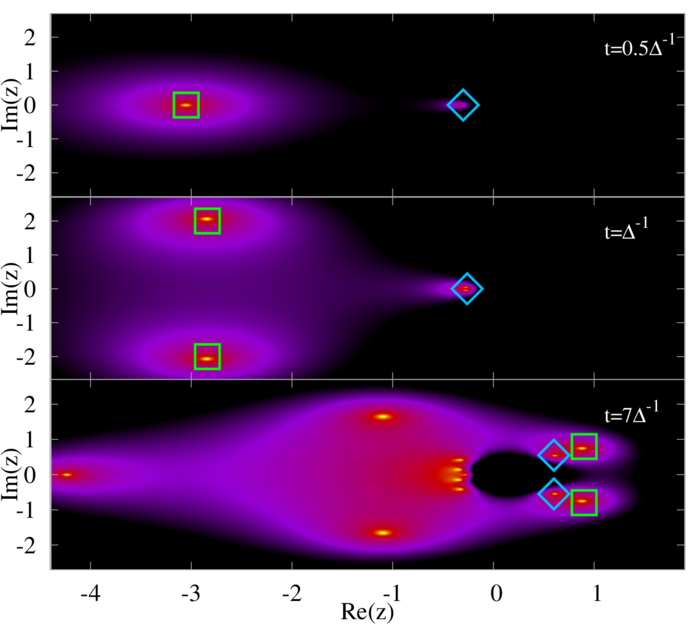
Figure 9: Short time behavior of the modulus of the inverse of the GF ($1/|Z(z,t)|$) as a function of the $z$ complex variable. At short times (top panel) we observe the zeros in the real negative axis, consistent with a non-interacting situation. At times of the order of $t\sim\Delta^{-1}$, the superconducting correlations become important and the zeros can appear as complex conjugate pairs. At longer times, the dominant DYLZs approach the measurement point, $z=1$. For clarity, we use the squares and diamonds to mark the dominant zeros. The parameter values are $\Gamma=2$, $\epsilon=0$, $\Delta=1$, $\phi=2$ and times $t=0.5$, $1$ and $7/\Delta$ (from top to bottom).

An alternative approach to the problem is provided by the analysis of the behavior of the DYLZs, which according to Eq. (7) fully characterize the transport properties of the system. In Fig. 9 we plot $1/|Z(z,t)|$, where the bright spots correspond to the DYLZs. At short times ($t\ll 1/\Delta$), the zeros are distributed along the negative real axis, a signature of uncorrelated electron transport Abanov and Ivanov (2008); Ivanov and Abanov (2010); Kambly et al. (2011); Utsumi et al. (2013). At intermediates times ($t\sim 1/\Delta$), superconducting correlations become important, and the zeros appear as complex conjugate pairs, shown by the green squares in the middle panel. At longer times ($t\gg 1/\Delta$), two pairs of complex conjugated zeros (represented by the symbols in the lower panel of Fig. 9) approach the measurement point $z=1$. These DYLZs will be referred to as dominant zeros, since they provide the main contribution to the cumulants given by Eq. (7). In Fig. 10 we show the accumulation of the DYLZs in the complex $z$-plane in the long time limit forming branches, for two different values of the tunneling rate. The dominant zeros tend to accumulate along the coarse grained result, given by Eq. (15), which describes two concentric circles (black lines). The description of the zeros located farther from the origin is poorer, since they may depend on details, such as the peak’s width, not included in the simplified model. The regions delimited by the two circles can be associated to states where the system is in a single phase, while the circles describe the phase coexistence lines Yang and Lee (1952); Lee and Yang (1952). The nature of each of the phases can be inferred from their transport properties. In the limit $t\to\infty$, the two circles tend to converge to the unitary one ($|z|=1$), leading to the coexistence of three phases at the measurement point, $z=1$, which thus becomes a triple point. This image is consistent with the one provided by the quasi-probabilities in Fig. 7. We would like to emphasize that the radius of the two circles in Fig. 10 is controlled by the divergences at the superconducting gap of the leads BCS density of states. A small broadening of these divergences, which, as discussed in Ref. Souto et al. (2016), causes the relaxation of the system towards the equilibrium stationary state, reduces the radius of the circle moving the transition point towards smaller $|z|$ values.

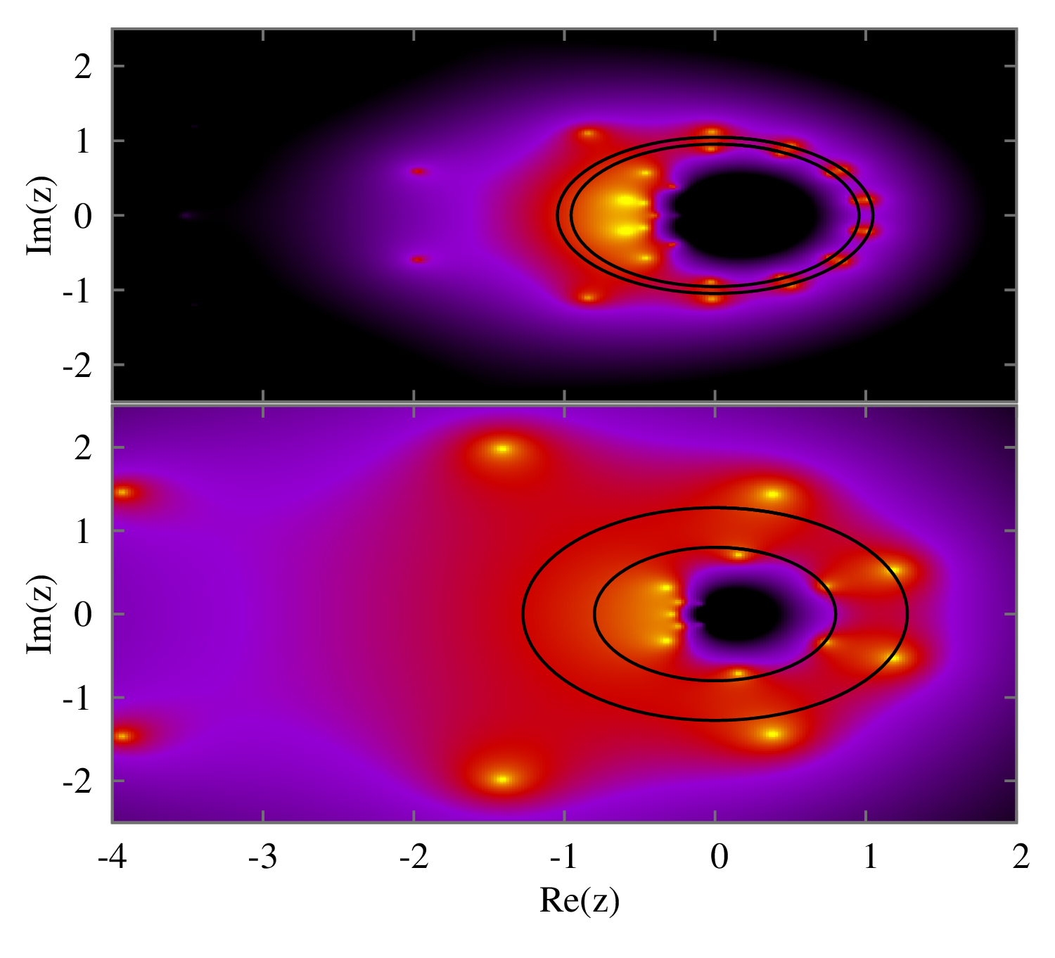
Figure 10: Long time $(t\sim 25/\Delta)$ behavior of $1/|Z|$ illustrating the accumulation of DYLZs around two circles which can be described by the coarse grained expression of Eq. (15). We show two different situations for $\Gamma=2$ (top panel) and $0.5$ (bottom panel). The other parameters are the same as in Fig. 9.

In Fig. 11 we show the shot noise computed from the dominant zeros, using Eq. (7). The time scaling of the shot noise is well described by the four dominant zeros marked with symbols in Fig. 9. This result is at variance with the case analyzed in Ref. Lee and Yang (1952), where only two phases coexist and thus only two dominant zeros are needed. In our case, however, two branches of DYLZs are needed, since $z=1$ becomes a triple point when $t\to\infty$.

Figure 11: Rebuilt noise evolution from the position of the dominant zeros. The green line corresponds to the noise evolution considering only the two dominant zeros (red squares in Fig. 9). For the blue line we consider 4 zeros (the two dominant and 2 subdominant ones, blue diamonds in Fig. 9), recovering the slope of the noise at short times. The dashed red line shows the convergence to the full result (black line) when considering a higher number of zeros (in this case around $10$).

Finally, in Fig. 12 we show the first two factorial cumulants (current and noise) as a function of the measurement point over the positive real $z$-axis, parametrized by the bias field $s$, see Eq. (10), for increasing times. The parameters are the same as in the lower panel of Fig. 10. In the factorial current, we observe a tendency to the formation of a jump at the measurement point, $s=0$, indicated by a dashed line in Fig. 12. This figure provides information about the nature of each of the phases: for $s>0$ (outside the two circles in Fig. 10) the current is positive, which for the choice of parameters, is a signature of the dominance of the ground state. In contrast, for $s<0$ (inside the two circles) the current is negative, indicating the dominance of the even excited state, while for $s\simeq 0$, i.e. between the two circles in Fig. 10 the current almost vanishes. On the other hand, the factorial noise tends to exhibit two maxima approaching the measurement point ($s\sim 0$) marked with arrows in the lower panel of Fig. 12, corresponding roughly to the condition $s+\alpha_{\pm}=1$ associated to the intersections with the phase coexistence lines (i.e. the circles indicated in Fig. 10). Again the increasing noise for $t\to\infty$ is a signature of phase coexistence as shown in Fig. 11. Although not shown, there is another divergence at $s\approx-1$ which corresponds to the point $z=0$, where a divergence naturally occurs due to the presence of charge transfer processes in the opposite direction to the mean current, see Eq. (14).

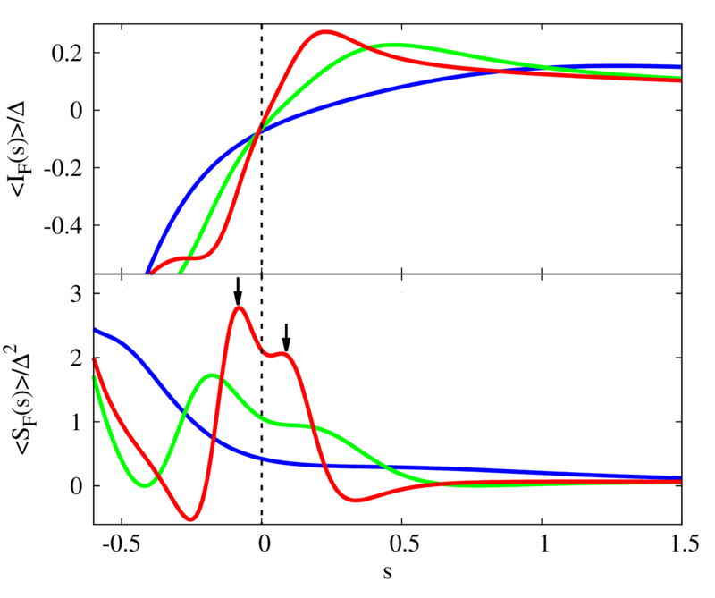
Figure 12: Factorial current (top) and noise (bottom panel) as a function of the bias field $s$. We show the evolution for three times, $t=10$ (blue), $25$ (green) and $50$ (red). The factorial current tends to exhibit jump around the measurement point (black dashed line) while the factorial noise tends to diverge at this point, which can be considered a signature of a dynamical first order transition. The factorial noise also exhibits two maxima, (marked with the arrows), associated to the intersection between the real $z$ axis and the two circles (see Fig. 10). The parameters are the same as in the lower panel of Fig. 10.

V Voltage biased junction

In this section we summarize the main results when a voltage bias is symmetrically applied to the junction $(\mu_{L}=-\mu_{R}=V/2)$. Some previous works have analyzed time resolved transport in superconducting nanojunctions, although focusing on the single particle properties Perfetto et al. (2009); Stefanucci et al. (2010); Albrecht et al. (2013); Weston and Waintal (2016); Taranko and Domanski (2017). The voltage bias can be incorporated in the superconducting phase, using a gauge transformation, leading to $\phi_{\nu}(t)=\phi_{\nu}(0)+\mu_{\nu}t$ ($\nu=L,R$).

V.1 Current evolution

In Fig. 13 we show the time evolution of the mean current for different bias voltages in the $\Gamma\gg\Delta$ regime. Differently from the phase-biased situation, the system relaxes to the stationary regime, with a relaxation time of the order of $t\sim\pi/V$. At longer times, the ac current oscillates around its mean value, represented in the right panel of Fig. 13. The oscillations with period $\pi/V$ correspond to the ac Josephson effect. In Fig. 14 we show the long time averaged (dc) current in the QPC regime for different transmission values. These results are in excellent agreement with the dc current obtained by standard stationary methods in Refs. Bratus et al. (1995); Averin and Bardas (1995); Cuevas et al. (1996), showed as dashed lines in the figure. This agreement is poorer in the low bias regime $V\lesssim\Delta/10$, where the convergence time to reach the steady state becomes larger and the calculation becomes computationally more demanding.

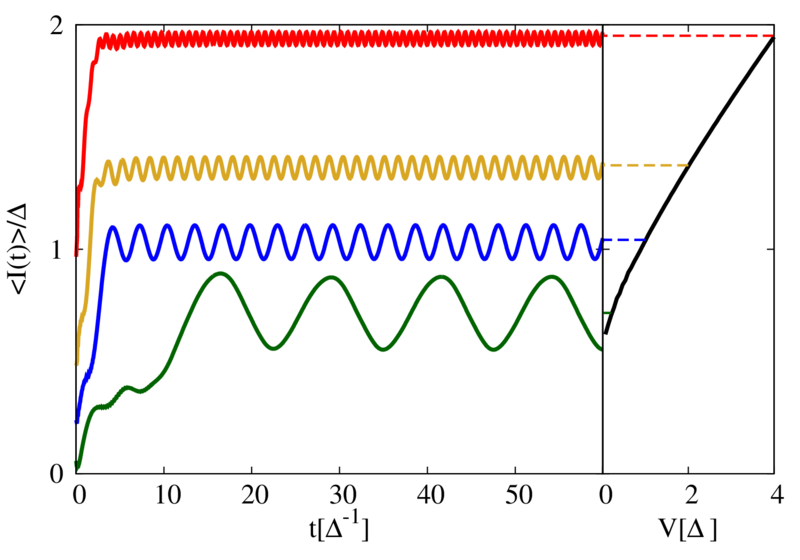
Figure 13: Time evolution of the current of a biased voltage nanojunction. We show the convergence to the stationary current as a function of the time, for $V=4$, $2$, $1$ and $0.25\Delta$, from top to bottom. We study the point contact regime, $\Gamma=10$ for a perfect transmitting junction ($\epsilon=0$ and $\Gamma_{L}=\Gamma_{R}=5$). In the right panel we show the convergence of the long time current Averin and Bardas (1995); Cuevas et al. (1996).

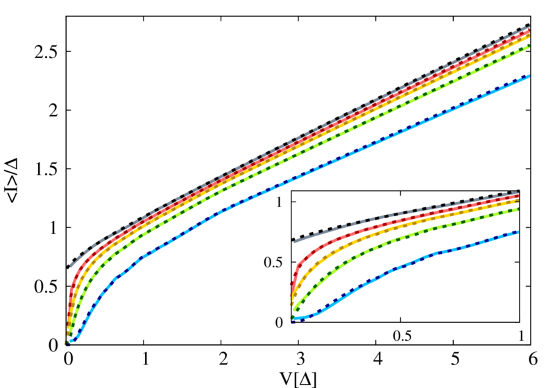
Figure 14: Long time averaged current for different transmissions ($\tau=1$, $0.99$, $0.98$, $0.96$ and $0.9$, from top to bottom) in the QPC regime (we have chosen $\Gamma=60\Delta$), compared to the dc stationary values (dashed lines) Averin and Bardas (1995); Cuevas et al. (1996). Inset: zoom on the low bias limit.

In Fig. 15 we show the dc current for a voltage biased junction in the QD regime. As in the QPC regime, we observe a remarkable agreement between the stationary calculation results Yeyati et al. (1997); Johansson et al. (1999); Yeyati et al. (2003) and the results obtained in this work in the long time limit. In the inset we show results for voltages smaller than the superconducting gap, exhibiting the expected subgap structure due to multiple Andreev reflections.

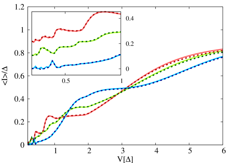
Figure 15: Long time averaged current for different positions, $\epsilon=0$ (red), $0.5$ (green) and $1$ (blue) in units of $\Delta$ (corresponding to transmissions values $\tau=1$, $0.8$ and $0.5$, respectively) for the QD regime (We have chosen $\Gamma=\Delta$), compared to the stationary values (dashed lines) Yeyati et al. (1997). Inset: zoom on the low bias limit. Curves are shifted up for clarity.

The convergence to the stationary situation is also illustrated in the time evolution of the occupied DOS in the QPC regime. In Fig. 16 we show the results for the case of a subgap voltage. Differently to the phase biased situation, the generated non-equilibrium quasi-particles relax when the ABSs approach the continuum of states. After a few cycles, the system reaches the stationary condition with the states pumping charge from the lower to the upper continuum of states Yeyati et al. (2003). In addition to the two main features, which can be associated to the evolution of the ABSs, more structure appears as replicas (or satellites) of the ABSs, due to their non-adiabatic evolution.

In the regime of $V>\Delta$, the evolution of the states becomes strongly non-adiabatic, being progressively difficult to resolve them in the DOS. In this regime, we observe a density of excited quasiparticles which is unable to relax in a time period. In the limit $V\gg\Delta$, we observe an almost homogeneous density of states, in the voltage window.

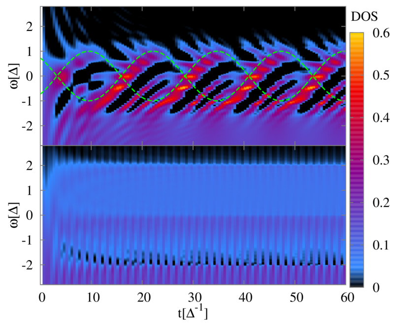
Figure 16: Time evolution of the occupied DOS for a bias voltage nanojunction in the QPC regime. We consider the perfect transmitting situation with two bias voltage, $V=0.25$ (top panel) and $2\Delta$ (bottom panel). For a small voltage we observe an adiabatic evolution of the states (showed by the green dashed line), exchanging charge at their crossing points. This charge is relaxed to the continuum of states, generating quasiparticles which are able to decay in a time period. For a voltage bigger than the superconducting gap (bottom panel), the dynamics of the ABSs cannot be resolved in time. In this situation, the generated quasiparticles are not able to relax in a time period, leading to an almost constant density of states in the voltage window.

For a non-perfect transmitting junction, an energy gap opens between the two ABSs which increases with decreasing $\tau$ as $\Delta_{A}=2\Delta\sqrt{1-\tau}$. This situation was discussed in the stationary and low voltage regime in Refs. Averin and Bardas (1995); Yeyati et al. (2003). In these works the authors demonstrated that the system evolves adiabatically except when $V\ll\Delta_{A}$ Landau-Zener transitions between the states, which happens with a probability $P=\exp[-\pi\Delta(1-\tau)/V]$. In Fig. 17 we show the time evolution of the occupied DOS for a non-perfect transmitting case with a voltage comparable (top panel) and much smaller (bottom panel) than the Andreev gap. In the first case, where the transition probability between the ABSs is $\sim 0.5$, we observe some finite population of the upper ABS. In the second case, the transition probability is negligible and the upper ABS remains almost unpopulated. Remarkably, we observe in both cases a convergence to the steady state, independently from the initial conditions.

Figure 17: Time evolution of the occupied DOS for a bias voltage nanojunction in the QPC regime, with transmissions $\tau=0.96$ (top panel) and $\tau=0.8$ (bottom panel), illustrating the convergence to the steady state independently from the value of the Andreev gap, $\Delta_{A}$. The remaining parameters are the same as in the top panel of Fig. 16.

V.2 Full Counting statistics and dynamical Yang-Lee zeros

In this subsection we present the FCS results for a voltage biased nanojunction after the sudden quench of the tunneling rates. In the upper panel of Fig. 18 we show the time evolution of the quasi-probabilities for the case $V<\Delta$. At very short times, smaller than the inverse of the Josephson frequency ($t\lesssim\pi/V$), three maxima are observed, i.e. a signature of a phase coexistence between the three many body states described above. At longer times, the slopes of the three peaks become equal, reflecting the convergence to the stationary regime characterized by the presence of a single quantum phase. The observation of these three maxima in the GF is related to the fact that the probabilities are accumulated quantities, but it is no longer reflecting a coexistence between three phases at long times. Although not shown, for voltages $V\gtrsim\Delta$, the initially trapped quasiparticles are able to relax before the ABSs are fully developed, avoiding the short time phase coexistence, and exhibiting a single quasiprobability maximum evolving linearly in time.

In the lower panel of Fig. 18 we show the time evolution of the current second cumulant, which can be related to the shot noise, for different bias voltages. At very short times, a linear increase in the noise is observed, consistent with the coexistence between the three phases. At longer times, when the phase coexistence disappears, the noise relaxes to the stationary situation. In the stationary regime, the shot noise exhibits an oscillatory behavior, where the maxima correspond to the subgap states approaching the gap edge leading to a maximum quasiparticle transfer.

Figure 18: Full counting statistics of a dc-biased junction For the same parameters as in the top panel of FIG. 16. In the top panel we show the time evolution of the probability after the contact formation. In the lower panel we show the evolution of the shot noise, which exhibits the linear divergence of the shot noise, due to phase coexistence, which is relax in the time when the state reaches the continuum and quasiparticles are relax.

The long time averaged shot noise behavior in the QPC regime is shown in Fig. 19, comparing our numerical results (solid lines) with the expected stationary value (dashed lines) Cuevas et al. (1999); Cuevas and Belzig (2003, 2004), for different transmission coefficients. As can be more clearly observed in the inset, where we show the shot noise in a enlarged scale for subgap voltages, the agreement with the stationary results is quite remarkable, except for the extremely small voltages where the relaxation time becomes too long to be reached in our simulations. The effect of a finite $\Gamma$ value has also some influence in the deviation between both calculations observed in the limit $V\to 0$ and $\tau\to 1$, as the stationary calculation corresponds strictly to the $\Gamma\to\infty$ limit. As already discussed in Refs. Cuevas et al. (1999); Cuevas and Belzig (2003, 2004), the Fano factor $\left\langle S\right\rangle/\left\langle I\right\rangle$ diverges in the $V\to 0$ limit, reflecting the increase in the effective transmitted charge due to the multiple Andreev reflection processes of increasing order.

In Fig. 20, we present the results for the long time averaged noise for the QD regime for three different level positions. In the inset we show the behavior for small voltages in an enlarged scale. To the best of our knowledge, these results have not been reported before and can be relevant to describe recent experiments Schönenberger . A detailed analysis of the observed features will be the subject of future work. It is worth remarking that, the time-resolved technique used in the present work allows us to obtain results for the steady state properties in parameters regimes which could be inaccessible for other methods.

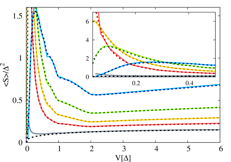
Figure 19: Long time averaged noise for different transmissions ($\tau=1$, $0.99$, $0.98$, $0.96$ and $0.9$, from top to bottom) in the QPC regime (We have chosen $\Gamma=60\Delta$), compared to the stationary values (dashed lines) Cuevas et al. (1999); Cuevas and Belzig (2003, 2004). Inset: zoom on the low biased junction.

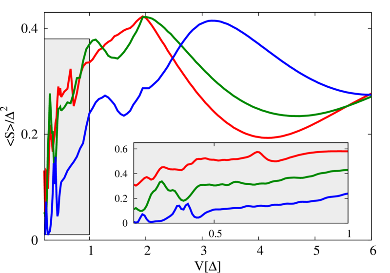
Figure 20: Long time averaged noise for different positions, $\epsilon_{0}=0$, $0.5$ and $1$ (corresponding to transmissions $\tau=1$, $0.8$ and $0.5$, respectively) in the QD regime (We have chosen $\Gamma=\Delta$). Inset: zoom on the low biased junction where the curves are shifted up for clarity. The parameters are the same as in Fig. 15.

In Fig. 21 we show the evolution of the DYLZs for a voltage biased junction with $V>\Delta$. As in the phase driven situation, the zeros appear as complex conjugate pairs for times of the order of the inverse of the superconducting gap (upper panel of Fig. 21). There is a relaxation of the initially trapped quasiparticles in the ABSs when they approach the continuum at $t\sim\pi/V$. This relaxation manifests itself in the appearance of an additional DYLZ in the negative real axis, marked with a black circle, which is absent in the phase biased case (middle panel of Fig. 9). When this zero becomes dominant (i.e. when it approaches the coordinates origin), the rest of the dynamical zeros approach the negative real axis (middle panel of Fig. 21). At longer times we observe that the zeros tend to converge to the negative real axis, showing a small imaginary part close to $z=0$, which decreases with increasing $\Gamma$. In the inset of the lower panel, we show in detail in a different scale the convergence of the DYLZs to the real axis, exhibiting a higher density close to $z=0$. This result is in qualitative agreement with the steady state zeros (shown as green dots in the lower panel of Fig. 21), computed using the CGF described in Refs. Cuevas and Belzig (2003, 2004) and shown as green dots in Fig. 21.

In Fig. 22 we show results for the DYLZs for a subgap bias. At short times (upper and middle panels) the zeros tend to converge to the unitary circle, which is a signature of a phase coexistence. Similarly to the case of voltages bigger than the superconducting gap, the DYLZs converge to their steady state, represented by the green lines in the lower panel of Fig. 22 and computed as above from the steady state results of Refs. Cuevas and Belzig (2003, 2004). The number of stationary branches is related to the number of different multiple Andreev processes contributing to the charge transport through the system at the corresponding bias, roughly given by $2\Delta/V$.

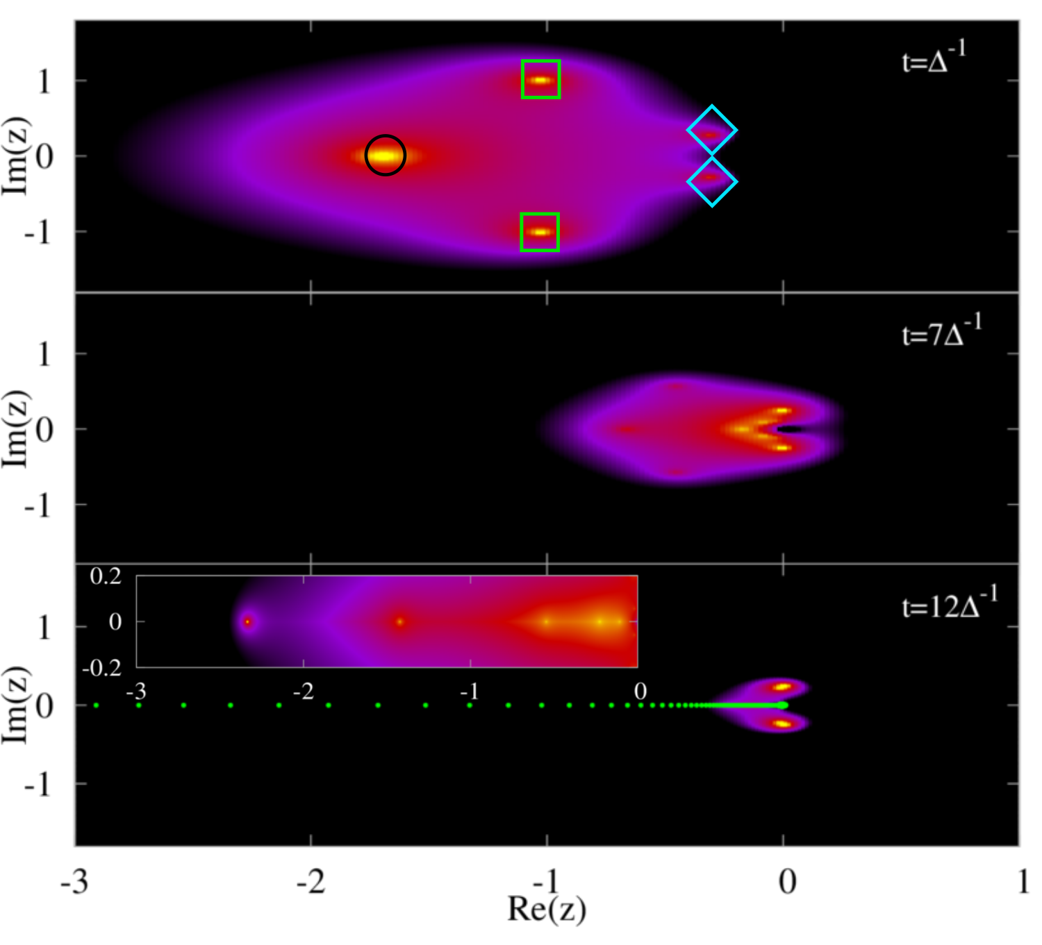
Figure 21: DYLZs in the voltage biased situation for a perfect transmitting junction, $\Gamma=10$, $V=2\Delta$. We observe how the phase coexistence is broken when the ABSs approach the continuum of states. In the top panel we show the result for the dominant zeros, marked as green squares and blue diamonds, as in the middle panel of Fig. 9. We observe an additional DYLZ related to the quasiparticle relaxation, marked with a black circle. For longer times, middle panel, their process become dominant and the zeros tend to converge to the negative real axis (bottom panel), showing and small imaginary part close to $z=0$, which decreases with increasing $\Gamma$. In the lower panel we show also the stationary result, computed using the CGF described in Refs. Cuevas and Belzig (2003, 2004), as green dots. The inset of the lower panel shows a zoom close to the real axis, in order to show the convergence of the DYLZs to the negative real axis, showing a higher density close to $z=0$, in qualitative agreement to the stationary result.

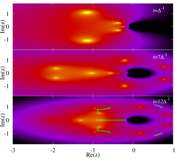
Figure 22: Same as Fig. 21, but with $V=0.25$. In the lower panel we compare the long time distribution of DYLZs with the stationary value, obtained from the CGF described in Refs. Cuevas and Belzig (2003, 2004)

VI Initialization after a dc pulse

VI.1 Current and ABS population

The convergence to the stationary regime in the voltage biased case can be used to initialize the system in a given state, by applying short dc voltage pulses to the junction. This mechanism resembles the antidote protocols proposed in Ref. Zgirski et al. (2011) to overcome quasiparticle poisoning. In Fig. 23 we show the occupied DOS after a bias voltage sudden switch off, in the low voltage regime $V\lesssim\Delta$. We observe how the subgap states evolve towards their stationary values with an almost thermal equilibrium population after the pulse. There is still some small probability of populating the upper state, given by the decaying quasiparticles from the upper continuum. It is important to note that the populated state is the one which has a positive dispersion relation (moving from negative to positive energies). It means that the upper ABS can be populated if the final phase is in the interval $\pi<\phi<2\pi$.

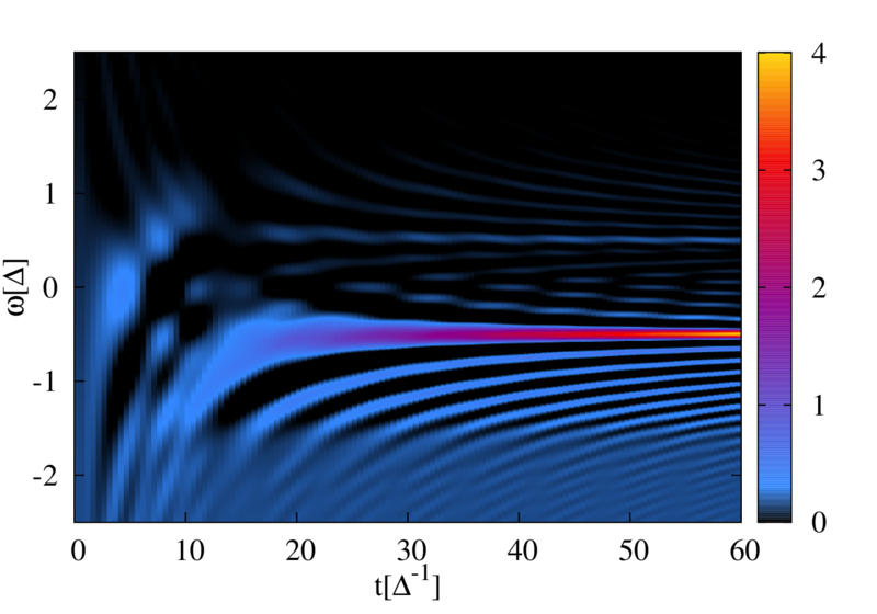
Figure 23: Formation of the ABSs after a dc pulse of amplitude $V=2$, initializing the system in the ground state with a final phase difference $\phi=2$. The other parameters are the same as in Fig. 13.

If a larger bias voltage is chosen ($V\gg\Delta$, $\Gamma$), a higher density of quasiparticles is generated and they are no longer relaxing to the expected thermal equilibrium situation after a suden voltage switch off. These two opposite behaviors are illustrated by the time evolution of the mean current in Fig. 24, showing a convergence to the thermal equilibrium situation for $V\lesssim\Delta$, and to memory-less quench dynamics for $V\gg\Delta$, $\Gamma$.

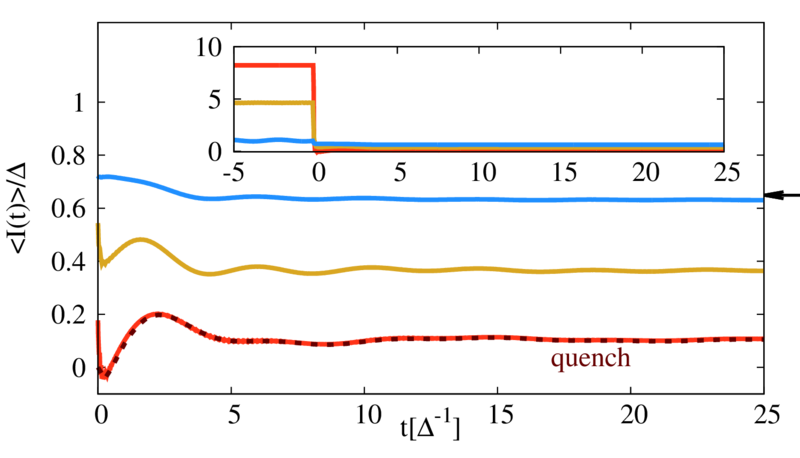
Figure 24: Current after a bias voltage switch off at $t=0$ and a phase difference $\phi=2$. From top to bottom, $V=2$, $16$ and $100\Delta$ showing the transition from the convergence to the stationary current represented by the black arrow ($V\lesssim\Delta$) to the quench result represented by the discontinuous line ($V\gg\Delta$). In the inset we show the current evolution during and just after the dc pulse.

VI.2 Full counting statistics and dynamical Yang-Lee zeros

The final state of the system can be better understood by analyzing the population of the many body states of the ABSs. This is illustrated in Fig. 25. For small voltage pulses (left panel), we observe a probability of populating the ground state (red line) of more than $\sim 90\%$. There is still some small probability of populating the odd state, given by the decaying quasiparticles in the upper continuum. Remarkably, there is no probability of populating the excited even state, meaning that the probability of the charge to be excited from the lower of the upper state is negligible in this regime. When the voltage is increased, we observe an evolution towards the universal quench result (right panel).

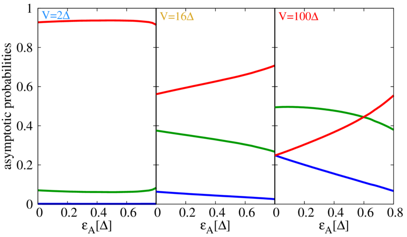
Figure 25: Long time populations of the many body states after the voltage switch off. We show the same three situations represented in Fig. 24, which illustrates the transition from the equilibrium state (left) to the quench result (right) as the voltage is increased.

Finally, in Fig. 26 we show the dynamical Yang-Lee zeros after a voltage quench. The system starts from the situation described in the lower panel of Fig. 21, with most of the DYLZs accumulated at two points close to the origin. With increasing time, we observe the generation of a single circle, converging to the unitary one at long times. This image is compatible with the two phases coexistence, as in the left panel of Fig. 25.

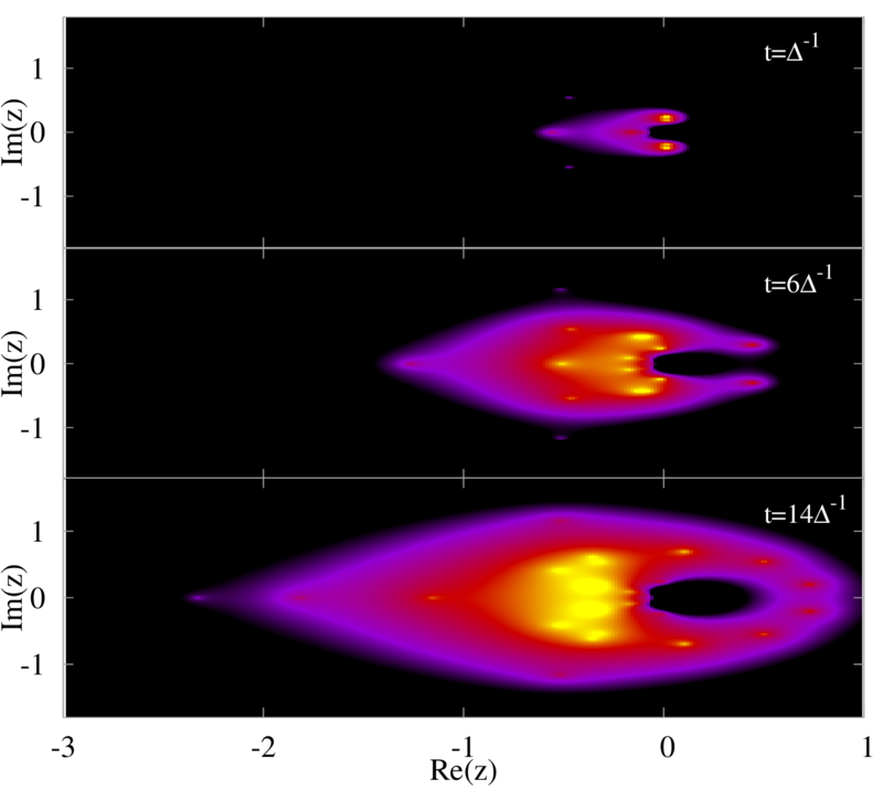
Figure 26: Poles after a voltage pulse. We observe how gradually the zeros tend to describe a single circle, signature of coexistence between two phases (see left panel of Fig. 25). Parameters: $\Gamma=10$, $\tau=1$, amplitude of the pulse $V=2\Delta$, final phase $\phi=2$.

VII Conclusions

We have presented a comprehensive analysis of the transient dynamics associated with the formation of superconducting nanojunctions. We have shown how information on the mean transport quantities and on the many body states population can be extracted from the generating function of the FCS. In particular, we have shown how these properties can be related to the evolution of the zeros of the generating function. We have studied the quench dynamics both in the cases of phase and voltage biased nanojunctions. In the first case the system typically gets trapped in a metastable state which is dependent on the switch-on rate of the connection to the leads. There is also a sensitivity to initial conditions which is more pronounced in the QD regime. In this case we have shown that either magnetic or non-magnetic metastable states can be produced. In the second case, the formation is accompanied by strong oscillations in the dot charge. Although the symmetrized current is not dependent on the initial conditions, their effect can be observed in the higher order cummulants and in the many body states population. In the voltage biased case the system converges to the steady state, independently from the initial conditions. The results thus obtained for current and noise are in quantitative agreement with those obtained using conventional stationary methods. We have also analyzed the possibility of coherently control the system state using a dc voltage drop. For small voltages ($V\lesssim\Delta$), the quasiparticles initially trapped in the system relax, and the system reaches the thermal equilibrium state. For large voltages, ($V\gg\Delta$), we recover the sudden connection result, providing a feasible experimental way to access the quench dynamics and to control the many body states population. We would like to remark that the method developed in this work can be used to study more complex situations which cannot be accessed by conventional stationary approaches, such as the one involving more terminals with non-commensurate applied bias Freyn et al. (2011); Jonckheere et al. (2013); Pfeffer et al. (2014) or the role of the interactions in the system.

Finally it is worth noticing the connection between our work and the recent intense activity on the phenomenon of many body localization (for recent reviews see Nandkishore and Huse (2015); Vasseur and Moore (2016)). Although these works are focused on closed many body systems, there is an analogy in the fact that the system does not necessarily reach the thermal equilibrium state in the absence of coupling to an external bath, preserving the memory of the initial state. We thus believe that our approach could be of interest also in connection to this fundamental field of research.

VIII Acknowledgments

We acknowledge discussions with W. Herrera,T. Jonckheere and J. P. Garrahan and financial support by Spanish MINECO through grant FIS2014-55486-P and the “María de Maeztu” Programme for Units of Excellence in R&D (MDM-2014-0377). We also acknowledge Santander Supercomputacion support group and the Spanish Supercomputing Network (RES) for providing access to the supercomputer Altamira at the Institute of Physics of Cantabria (IFCA-CSIC).

Appendix A Analytical results for the mean charge in the central region

For the calculation of the mean charge and current it is convenient to use the Keldysh formalism in the triangular form, where only the retarded, advanced and Keldysh $+-$ components are involved in the Dyson equation. For an abrupt connection between the leads and the central region, the retarded (advanced) Green functions have a simple form in Nambu space

$$\hat{G}^{R(A)}(t,t^{\prime})=\theta(t)\theta(t^{\prime})\hat{G}_{stat}^{R(A)}(t-t^{\prime})\,,$$ (17)

where $\hat{G}_{stat}^{R(A)}(t-t^{\prime})$ denotes the stationary retarded (advanced) Green function. This expression is completely general for an abrupt connection in the absence of interactions, and it reduces to the expression provided in Ref. Jauho et al. (1994) for normal electrodes. In the frequency domain the stationary retarded (advanced) Green function can be written as

$$\hat{G}_{stat}^{R(A)}(\omega)=\left(\begin{array}[]{cc}\omega-\epsilon_{0}-\Gamma g_{11}^{R(A)}&(\Gamma_{L}e^{i\phi_{L}}+\Gamma_{R}e^{i\phi_{R}})g_{12}^{R(A)}\\ (\Gamma_{L}e^{-i\phi_{L}}+\Gamma_{R}e^{-i\phi_{R}})g_{12}^{R(A)}&\omega+\epsilon_{0}-\Gamma g_{22}^{R(A)}\end{array}\right)^{-1}$$ (18)

where $g^{R(A)}_{\alpha\beta}$ are the BCS Green functions of the uncoupled electrodes Martín-Rodero and Yeyati (2011).

$\hat{G}_{stat}^{R(A)}(\omega)$ have poles for $|\omega|\leq\Delta$ plane, which correspond to the ABSs at $\pm\epsilon_{A}(\phi)$. In the limit $\Gamma/\Delta\ll 1$ the contribution from the continuum spectrum for $|\omega|>\Delta$ becomes negligible and $\hat{G}^{R,A}(t,t^{\prime})$ can be approximated by

$$\hat{G}^{R(A)}(t,t^{\prime})\simeq\theta(t)\theta(t^{\prime})\sum_{\pm}\left(\begin{array}[]{cc}p_{\pm}&\pm p_{12}\\ \pm p^{*}_{12}&p_{\pm}\end{array}\right)e^{\pm i\epsilon_{A}(t-t^{\prime})}$$ (19)

where $|p_{12}|=\sqrt{p_{+}p_{-}}$. The ABS energies and the weights $p_{\pm}$ adopt a simple form when $\epsilon_{0}<\Gamma$, i.e. $\epsilon_{A}=\sqrt{\epsilon_{0}^{2}+\Gamma^{2}\cos^{2}(\phi/2)+(\Gamma_{L}-\Gamma_{R})^{2}\sin^{2}(\phi/2)}$ and

$$P_{\pm}=\frac{\Delta}{2\sqrt{\Delta^{2}+\epsilon_{A}^{2}}}\left(1-\frac{\Gamma}{\Delta}\mp\frac{\epsilon_{0}}{\epsilon_{A}}\right)\,.$$ (20)

The time-dependent level charge can then be obtained through the Dyson equation for the Keldysh Green function $\hat{G}^{+-}$,

$$\hat{G}^{+-}=\hat{G}^{R}\hat{\Sigma}^{+-}\hat{G}^{A}+\left(1+\hat{G}^{R}\hat{\Sigma}^{R}\right)\hat{g}_{0}^{+-}\left(1+\hat{\Sigma}^{A}\hat{G}^{A}\right)\,,$$ (21)

where $\hat{g}_{0}^{+-}$ is the Keldysh Green function of the uncoupled central level in Nambu space,

$$\hat{g}_{0}^{+-}(t,t^{\prime})=ie^{-i\epsilon_{0}(t-t^{\prime})}\left(\begin{array}[]{cc}n_{\uparrow}(0)&0\\ 0&1-n_{\downarrow}(0)\end{array}\right)\,.$$ (22)

$\hat{\Sigma}^{+-}$ is the self energy coupling the level to the electrodes,

$$\hat{\Sigma}^{+-}=\sum_{\nu}\left(G^{R}\Sigma^{R}\right)_{0\nu}g_{\nu}^{+-}\left(\Sigma^{A}G^{A}\right)_{\nu 0}\,,$$ (23)

where $g_{\nu}^{+-}(t,t^{\prime})$ are the BCS Green functions of the superconducting electrodes, given in the supplemental material of Ref. Souto et al. (2016).

For simplicity, the time arguments in Eq. (21) have not been included and all the products represent time convolutions. For an initial condition $(n_{\uparrow}(0),n_{\downarrow}(0))=(0,1)$ only the first term in the equation contributes to $n_{\uparrow}(t)$. Substitution of Eq. 19 in Eq. 21 then yields

$$n_{\uparrow}(t) = \sum_{\pm}n_{\pm}(t)+n_{+-}$$

$$n_{\pm}(t) = -\frac{2p_{\pm}}{\pi}\int_{-\infty}^{-\Delta}\frac{\omega\Gamma\mp 4p_{+}p_{-}\Delta\cdot\epsilon_{A}}{\sqrt{\omega^{2}-\Delta^{2}}\omega_{\mp}}\left[1-\cos\left(\omega_{\mp}t\right)\right]d\omega$$

$$n_{+-} = \frac{2(p_{+}-p_{-})}{\pi}\int_{-\infty}^{-\Delta}\frac{4p_{+}p_{-}\Delta\cdot\epsilon_{A}}{\omega_{+}\omega_{-}\sqrt{\omega^{2}-\Delta^{2}}}\left[1+\cos\left(2\epsilon_{A}t\right)-\cos(\omega_{+}t)-\cos(\omega_{-}t)\right]d\omega$$ (24)

where $\omega_{\pm}=\omega\pm\epsilon_{A}$ (the spin down population is simply given in this limit by $n_{\downarrow}(t)=1-n_{\uparrow}(t)$). As can be observed, the central level occupation is composed by contributions from the upper and lower ABS denoted by $n_{\pm}$ and predicts for $\Gamma\lesssim\Delta$ and this initial condition a long time magnetic solution. Additionally there is an interference term $n_{+-}$, which vanishes for the electron-hole symmetric situation ($\epsilon_{0}=0$). This last term is well approximate at times $t>1/\Delta$ as Souto et al. (2016)

$$n_{+-}(t)\simeq-\frac{\epsilon_{0}}{\pi\Delta}\left(1-\frac{\epsilon_{0}^{2}}{\epsilon_{A}^{2}}\right)\left[1+\cos(2\epsilon_{A}t)+\sqrt{\frac{2\pi}{\Delta\cdot t}}\cos(\epsilon_{A}t)\sin\left(\Delta\cdot t-\frac{\pi}{4}\right)\right]$$ (25)

For a different initial condition, $(n_{\uparrow}(0),n_{\downarrow}(0))=(0,0)$ or $(n_{\uparrow}(0),n_{\downarrow}(0))=(1,1)$ there is a contribution from the second term in Eq. 21. For an initially empty level the solution is non-magnetic ($n_{\uparrow}(t)=n_{\downarrow}(t)$), and we have $n_{\sigma}(t)=\sum_{\pm}n_{\pm}(t)+n_{+-}+n_{\sigma,00}$ where

$$n_{\sigma,00}(t)=2\left|p_{12}\right|^{2}\left[1-\cos(2\epsilon_{A}t)\right]\,,$$ (26)

which describes undamped oscillations (see Fig. 3). Similar expressions can be derived for the other initial fully occupied configuration.

Appendix B Interpretation in terms of rate equations

A simple interpretation of the numerical results for the asymptotic probabilities $P_{\pm}(t)$ and $P_{odd}(t)=P_{odd,\uparrow}(t)+P_{odd,\downarrow}(t)$ can be obtained assuming that they are governed by simple rate equations with time dependent rates. More precisely, these equations are

$$\frac{dP_{-}}{dt} = -2\Gamma_{odd}(t)P_{-}+\Gamma_{-}(t)P_{odd}$$

$$\frac{dP_{odd}}{dt} = 2\Gamma_{odd}(t)P_{-}-\left[\Gamma_{-}(t)+\Gamma_{+}(t)\right]P_{odd}+2\Gamma_{odd}(t)P_{+}$$

$$\frac{dP_{+}}{dt} = \Gamma_{+}(t)P_{odd}-2\Gamma_{odd}(t)P_{+}\;,$$ (27)

where $\Gamma_{odd}(t)$ and $\Gamma_{\pm}(t)$ are the time-dependent rates for transitions between states. Although these quantities are not well defined, an estimate based on perturbation theory would suggest that they should be inversely proportional to the energy distance from the lower gap edge to the corresponding state. For $\Gamma/\Delta\gg 1$ the rates can be considered as time independent and approximated as $\Gamma_{odd}\approx\Gamma^{2}/\Delta$ and $\Gamma_{\pm}\approx\Gamma^{2}/(\Delta\pm\epsilon_{A})$. Using these estimates one obtains the results indicated by the dashed lines in the left panel of Fig. 5 of the main text.

Appendix C Bidirectional Poisson distribution

In this section we show the calculation details for the bidirectional Poisson distribution, also known in the literature as birth-death processes Gardiner (2009). We assume that, starting from an initial population, $n$, there is a birth rate (d) and a death rate (d), which connects the subspaces with different population (see Fig. 27). The distribution supposes that birth and death processes occur with a fixed probability, independently from the history of the system. In our case, the population will describe the number of electrons transfer through the junction, being the initial population $n=0$. Then, a positive (negative) population is interpreted as a net charge flowing from the left (right) electrode to the right (left) one. The results for the short time dynamics can be found in the lower panel of Fig. 4, where equal birth and death probability rates are considered ($b=d$).

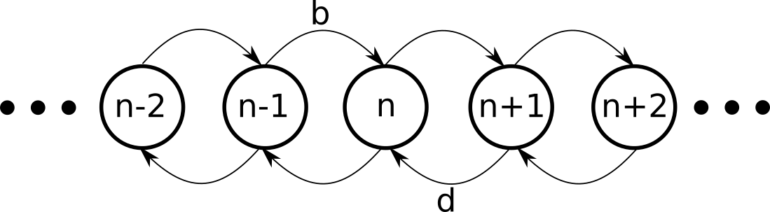
Figure 27: Scheme of the birth-death process. The birth process (which has a probability $b$), allows to go from $n$ to $n+1$ charges transferred through the junction. In the short time limit, we consider $b=d$, due to the absence of bias voltage.

The calculation of the population is done in the following way. We start with an initial population $P(0)=(\ldots,0,1,0,\ldots)^{T}$. The recursive expression for computing the probability distribution can be written as $P(t+dt)=M\cdot P(t)$, being

$$M=\left(\begin{array}[]{cccc}\ddots&\ddots&&\\ \ddots&a&d\,dt&\\ &d\,dt&a&\ddots\\ &&\ddots&\ddots\end{array}\right),$$

and $a=1-(b+d)dt$ is the probability of staying at the same subspace after $dt$. The discontinuous dots mean that we consider enough probabilities to make the border effects negligible. In our problem, the short time state of the system is fully characterize by the parameter $n_{\rightarrow}(t)=b\,dt=d\,dt$, which is the mean charge transfer in one of the directions of the junction (without considering charges flowing in the opposite direction). For fitting the Fig. 7 at short times, we have taken $n_{\rightarrow}(t)\sim 1$ for the discontinuous line and $n_{\rightarrow}(t)\sim 3$ for the dotted one. Then, the mean number of electrons crossing the junction needed necessary for the ABS to be formed is surprisingly small (they are of the order of $3$ electrons crossing the junction in both directions of the junction).

References

- Devoret and Schoelkopf (2013) M. H. Devoret and R. J. Schoelkopf, “Superconducting circuits for quantum information: An outlook,” Science 339, 1169–1174 (2013).
- Alicea (2012) Jason Alicea, “New directions in the pursuit of majorana fermions in solid state systems,” Reports on Progress in Physics 75, 076501 (2012).
- Beenakker (2015) C. W. J. Beenakker, “Random-matrix theory of majorana fermions and topological superconductors,” Rev. Mod. Phys. 87, 1037–1066 (2015).
- Plugge et al. (2017) Stephan Plugge, Asbjørn Rasmussen, Reinhold Egger, and Karsten Flensberg, “Majorana box qubits,” New Journal of Physics 19, 012001 (2017).
- Martinis et al. (2009) John M. Martinis, M. Ansmann, and J. Aumentado, “Energy decay in superconducting josephson-junction qubits from nonequilibrium quasiparticle excitations,” Phys. Rev. Lett. 103, 097002 (2009).
- Catelani et al. (2011) G. Catelani, R. J. Schoelkopf, M. H. Devoret, and L. I. Glazman, “Relaxation and frequency shifts induced by quasiparticles in superconducting qubits,” Phys. Rev. B 84, 064517 (2011).
- Ristè et al. (2013) D. Ristè, C. C. Bultink, M. J. Tiggelman, R. N. Schouten, K. W. Lehnert, and L. DiCarlo, “Millisecond charge-parity fluctuations and induced decoherence in a superconducting transmon qubit,” Nat. Commun. 4, 1913 (2013).
- Avriller and Pistolesi (2015) R. Avriller and F. Pistolesi, “Andreev bound-state dynamics in quantum-dot josephson junctions: A washing out of the transition,” Phys. Rev. Lett. 114, 037003 (2015).
- Rainis and Loss (2012) Diego Rainis and Daniel Loss, “Majorana qubit decoherence by quasiparticle poisoning,” Phys. Rev. B 85, 174533 (2012).
- Colbert and Lee (2014) Jacob R. Colbert and Patrick A. Lee, “Proposal to measure the quasiparticle poisoning time of majorana bound states,” Phys. Rev. B 89, 140505 (2014).
- Bespalov et al. (2016) Anton Bespalov, Manuel Houzet, Julia S. Meyer, and Yuli V. Nazarov, “Theoretical model to explain excess of quasiparticles in superconductors,” Phys. Rev. Lett. 117, 117002 (2016).
- Albrecht et al. (2017) S. M. Albrecht, E. B. Hansen, A. P. Higginbotham, F. Kuemmeth, T. S. Jespersen, J. Nygård, P. Krogstrup, J. Danon, K. Flensberg, and C. M. Marcus, “Transport signatures of quasiparticle poisoning in a majorana island,” Phys. Rev. Lett. 118, 137701 (2017).
- Zgirski et al. (2011) M. Zgirski, L. Bretheau, Q. Le Masne, H. Pothier, D. Esteve, and C. Urbina, “Evidence for long-lived quasiparticles trapped in superconducting point contacts,” Phys. Rev. Lett. 106, 257003 (2011).
- Olivares et al. (2014) D. G. Olivares, A. L. Yeyati, L. Bretheau, Ç. Ö. Girit, H. Pothier, and C. Urbina, “Dynamics of quasiparticle trapping in andreev levels,” Phys. Rev. B 89, 104504 (2014).
- Padurariu and Nazarov (2012) C. Padurariu and Yu. V. Nazarov, “Spin blockade qubit in a superconducting junction,” EPL (Europhysics Letters) 100, 57006 (2012).
- Nazarov and Yaroslav (2009) Yuli V Nazarov and Blanter M Yaroslav, Quantum transport: introduction to nanoscience (Cambridge Univ. Press, Cambridge, 2009).
- Fève et al. (2007) G. Fève, A. Mahé, J.-M. Berroir, T. Kontos, B. Plaçais, D. C. Glattli, A. Cavanna, B. Etienne, and Y. Jin, “An on-demand coherent single-electron source,” Science 316, 1169–1172 (2007).
- Bocquillon et al. (2013) E. Bocquillon, V. Freulon, J.-M Berroir, P. Degiovanni, B. Plaçais, A. Cavanna, Y. Jin, and G. Fève, “Coherence and indistinguishability of single electrons emitted by independent sources,” Science 339, 1054–1057 (2013).
- Dubois et al. (2013) J. Dubois, T. Jullien, F. Portier, P. Roche, A. Cavanna, Y. Jin, W. Wegscheider, P. Roulleau, and D. C. Glattli, “Minimal-excitation states for electron quantum optics using levitons,” Nature (London) 502, 659–663 (2013).
- Garrahan and Lesanovsky (2010) Juan P. Garrahan and Igor Lesanovsky, “Thermodynamics of quantum jump trajectories,” Phys. Rev. Lett. 104, 160601 (2010).
- Heyl et al. (2013) M. Heyl, A. Polkovnikov, and S. Kehrein, “Dynamical quantum phase transitions in the transverse-field ising model,” Phys. Rev. Lett. 110, 135704 (2013).
- Karrasch and Schuricht (2013) C. Karrasch and D. Schuricht, “Dynamical phase transitions after quenches in nonintegrable models,” Phys. Rev. B 87, 195104 (2013).
- Hickey et al. (2013a) James M. Hickey, Sam Genway, Igor Lesanovsky, and Juan P. Garrahan, “Time-integrated observables as order parameters for full counting statistics transitions in closed quantum systems,” Phys. Rev. B 87, 184303 (2013a).
- Yang and Lee (1952) C. N. Yang and T. D. Lee, “Statistical theory of equations of state and phase transitions. i. theory of condensation,” Phys. Rev. 87, 404–409 (1952).
- Lee and Yang (1952) T. D. Lee and C. N. Yang, “Statistical theory of equations of state and phase transitions. ii. lattice gas and ising model,” Phys. Rev. 87, 410–419 (1952).
- Utsumi et al. (2013) Y. Utsumi, O. Entin-Wohlman, A. Ueda, and A. Aharony, “Full-counting statistics for molecular junctions: Fluctuation theorem and singularities,” Phys. Rev. B 87, 115407 (2013).
- Peng et al. (2015) Xinhua Peng, Hui Zhou, Bo-Bo Wei, Jiangyu Cui, Jiangfeng Du, and Ren-Bao Liu, “Experimental observation of lee-yang zeros,” Phys. Rev. Lett. 114, 010601 (2015).
- Ivanov and Abanov (2013) Dmitri A. Ivanov and Alexander G. Abanov, “Characterizing correlations with full counting statistics: Classical ising and quantum spin chains,” Phys. Rev. E 87, 022114 (2013).
- Souto et al. (2016) R. S. Souto, A. Martín-Rodero, and A. L. Yeyati, “Andreev bound states formation and quasiparticle trapping in quench dynamics revealed by time-dependent counting statistics,” Phys. Rev. Lett. 117, 267701 (2016).
- Flindt and Garrahan (2013) Christian Flindt and Juan P. Garrahan, “Trajectory phase transitions, lee-yang zeros, and high-order cumulants in full counting statistics,” Phys. Rev. Lett. 110, 050601 (2013).
- Hickey et al. (2014) James M. Hickey, Christian Flindt, and Juan P. Garrahan, “Intermittency and dynamical lee-yang zeros of open quantum systems,” Phys. Rev. E 90, 062128 (2014).
- Brandner et al. (2017) Kay Brandner, Ville F. Maisi, Jukka P. Pekola, Juan P. Garrahan, and Christian Flindt, “Experimental determination of dynamical lee-yang zeros,” Phys. Rev. Lett. 118, 180601 (2017).
- Flindt et al. (2009) C. Flindt, C. Fricke, F. Hohls, T. Novotný, K. Netočný, T. Brandes, and R.J. Haug, “Universal oscillations in counting statistics,” Proceedings of the National Academy of Sciences of the United States of America 106, 10116–10119 (2009).
- Levitov (2002) L.S. Levitov, Quantum noise in Mesoscopic Physics (Kluwer Academic Press, New York, 2002).
- Cohen et al. (2014) Guy Cohen, Emanuel Gull, David R. Reichman, and Andrew J. Millis, “Green’s functions from real-time bold-line monte carlo calculations: Spectral properties of the nonequilibrium anderson impurity model,” Phys. Rev. Lett. 112, 146802 (2014).
- Chen et al. (2016) Hsing-Ta Chen, Guy Cohen, Andrew J. Millis, and David R. Reichman, “Anderson-holstein model in two flavors of the noncrossing approximation,” Phys. Rev. B 93, 174309 (2016).
- Kamenev (2011) A. Kamenev, Field Theory of Non-Equilibrium Systems (Cambridge University Press, 2011).
- Esposito et al. (2009) Massimiliano Esposito, Upendra Harbola, and Shaul Mukamel, “Nonequilibrium fluctuations, fluctuation theorems, and counting statistics in quantum systems,” Rev. Mod. Phys. 81, 1665–1702 (2009).
- Tang et al. (2014) Gao-Min Tang, Fuming Xu, and Jian Wang, “Waiting time distribution of quantum electronic transport in the transient regime,” Phys. Rev. B 89, 205310 (2014).
- Tang and Wang (2014) Gao-Min Tang and Jian Wang, “Full-counting statistics of charge and spin transport in the transient regime: A nonequilibrium green’s function approach,” Phys. Rev. B 90, 195422 (2014).
- Seoane Souto et al. (2015) R. Seoane Souto, R. Avriller, R. C. Monreal, A. Martín-Rodero, and A. Levy Yeyati, “Transient dynamics and waiting time distribution of molecular junctions in the polaronic regime,” Phys. Rev. B 92, 125435 (2015).
- Belzig and Nazarov (2001) W. Belzig and Yu. V. Nazarov, “Full counting statistics of electron transfer between superconductors,” Phys. Rev. Lett. 87, 197006 (2001).
- Shelankov and Rammer (2003) A. Shelankov and J. Rammer, “Charge transfer counting statistics revisited,” EPL (Europhysics Letters) 63, 485 (2003).
- Hofer and Clerk (2016) Patrick P. Hofer and A. A. Clerk, “Negative full counting statistics arise from interference effects,” Phys. Rev. Lett. 116, 013603 (2016).
- Hickey et al. (2013b) James M. Hickey, Christian Flindt, and Juan P. Garrahan, “Trajectory phase transitions and dynamical lee-yang zeros of the glauber-ising chain,” Phys. Rev. E 88, 012119 (2013b).
- Seoane Souto et al. (2017) R. Seoane Souto, A. Martín-Rodero, and A. Levy Yeyati, “Analysis of universality in transient dynamics of coherent electronic transport,” Fortschr. Phys. 65, 1600062–n/a (2017).
- Abramowitz and Stegun (1964) M. Abramowitz and I.A. Stegun, Handbook of Mathematical Functions: With Formulas, Graphs, and Mathematical Tables, Applied mathematics series (Dover Publications, 1964).
- Berry (2005) M.V Berry, “Universal oscillations of high derivatives,” Proc. R. Soc. of London A 461, 1735–1751 (2005).
- Flindt et al. (2010) Christian Flindt, Tomá š Novotný, Alessandro Braggio, and Antti-Pekka Jauho, “Counting statistics of transport through coulomb blockade nanostructures: High-order cumulants and non-markovian effects,” Phys. Rev. B 82, 155407 (2010).
- Kambly et al. (2011) Dania Kambly, Christian Flindt, and Markus Büttiker, “Factorial cumulants reveal interactions in counting statistics,” Phys. Rev. B 83, 075432 (2011).
- Stegmann et al. (2015) Philipp Stegmann, Björn Sothmann, Alfred Hucht, and Jürgen König, “Detection of interactions via generalized factorial cumulants in systems in and out of equilibrium,” Phys. Rev. B 92, 155413 (2015).
- Stegmann and König (2016) Philipp Stegmann and Jürgen König, “Short-time counting statistics of charge transfer in coulomb-blockade systems,” Phys. Rev. B 94, 125433 (2016).
- Zazunov et al. (2014) A. Zazunov, A. Brunetti, A. L. Yeyati, and R. Egger, “Quasiparticle trapping, andreev level population dynamics, and charge imbalance in superconducting weak links,” Phys. Rev. B 90, 104508 (2014).
- Abanov and Ivanov (2008) A. G. Abanov and D. A. Ivanov, “Allowed charge transfers between coherent conductors driven by a time-dependent scatterer,” Phys. Rev. Lett. 100, 086602 (2008).
- Ivanov and Abanov (2010) D. A. Ivanov and A. G. Abanov, “Phase transitions in full counting statistics for periodic pumping,” EPL (Europhysics Letters) 92, 37008 (2010).
- Perfetto et al. (2009) Enrico Perfetto, Gianluca Stefanucci, and Michele Cini, “Equilibrium and time-dependent josephson current in one-dimensional superconducting junctions,” Phys. Rev. B 80, 205408 (2009).
- Stefanucci et al. (2010) Gianluca Stefanucci, Enrico Perfetto, and Michele Cini, “Time-dependent quantum transport with superconducting leads: A discrete-basis kohn-sham formulation and propagation scheme,” Phys. Rev. B 81, 115446 (2010).
- Albrecht et al. (2013) K.F. Albrecht, H. Soller, L. Mühlbacher, and A. Komnik, “Transient dynamics and steady state behavior of the anderson–holstein model with a superconducting lead,” Phys. E 54, 15–23 (2013).
- Weston and Waintal (2016) Joseph Weston and Xavier Waintal, “Linear-scaling source-sink algorithm for simulating time-resolved quantum transport and superconductivity,” Phys. Rev. B 93, 134506 (2016).
- Taranko and Domanski (2017) R. Taranko and T. Domanski, “How long does it take to form the andreev quasiparticles?” arXiv:1705.08755 (2017).
- Bratus et al. (1995) E. N. Bratus, V. S. Shumeiko, and G. Wendin, “Theory of subharmonic gap structure in superconducting mesoscopic tunnel contacts,” Phys. Rev. Lett. 74, 2110–2113 (1995).
- Averin and Bardas (1995) D. Averin and A. Bardas, “ac josephson effect in a single quantum channel,” Phys. Rev. Lett. 75, 1831–1834 (1995).
- Cuevas et al. (1996) J. C. Cuevas, A. Martín-Rodero, and A. Levy Yeyati, “Hamiltonian approach to the transport properties of superconducting quantum point contacts,” Phys. Rev. B 54, 7366–7379 (1996).
- Yeyati et al. (1997) A. Levy Yeyati, J. C. Cuevas, A. López-Dávalos, and A. Martín-Rodero, “Resonant tunneling through a small quantum dot coupled to superconducting leads,” Phys. Rev. B 55, R6137–R6140 (1997).
- Johansson et al. (1999) G. Johansson, E. N. Bratus, V. S. Shumeiko, and G. Wendin, “Resonant multiple andreev reflections in mesoscopic superconducting junctions,” Phys. Rev. B 60, 1382–1393 (1999).
- Yeyati et al. (2003) A. Levy Yeyati, A. Martín-Rodero, and E. Vecino, “Nonequilibrium dynamics of andreev states in the kondo regime,” Phys. Rev. Lett. 91, 266802 (2003).
- Cuevas et al. (1999) J. C. Cuevas, A. Martín-Rodero, and A. Levy Yeyati, “Shot noise and coherent multiple charge transfer in superconducting quantum point contacts,” Phys. Rev. Lett. 82, 4086–4089 (1999).
- Cuevas and Belzig (2003) J. C. Cuevas and W. Belzig, “Full counting statistics of multiple andreev reflections,” Phys. Rev. Lett. 91, 187001 (2003).
- Cuevas and Belzig (2004) J. C. Cuevas and W. Belzig, “dc transport in superconducting point contacts: A full-counting-statistics view,” Phys. Rev. B 70, 214512 (2004).
- (70) Christian Schönenberger, Private communication .
- Freyn et al. (2011) Axel Freyn, Benoit Douçot, Denis Feinberg, and Régis Mélin, “Production of nonlocal quartets and phase-sensitive entanglement in a superconducting beam splitter,” Phys. Rev. Lett. 106, 257005 (2011).
- Jonckheere et al. (2013) T. Jonckheere, J. Rech, T. Martin, B. Douçot, D. Feinberg, and R. Mélin, “Multipair dc josephson resonances in a biased all-superconducting bijunction,” Phys. Rev. B 87, 214501 (2013).
- Pfeffer et al. (2014) A. H. Pfeffer, J. E. Duvauchelle, H. Courtois, R. Mélin, D. Feinberg, and F. Lefloch, “Subgap structure in the conductance of a three-terminal josephson junction,” Phys. Rev. B 90, 075401 (2014).
- Nandkishore and Huse (2015) R Nandkishore and D A Huse, “Nonequilibrium fluctuations, fluctuation theorems, and counting statistics in quantum systems,” Ann. Rev. Condens. Matter Phys. 6, 201 (2015).
- Vasseur and Moore (2016) Romain Vasseur and Joel E Moore, “Nonequilibrium quantum dynamics and transport: from integrability to many-body localization,” Journal of Statistical Mechanics: Theory and Experiment 2016, 064010 (2016).
- Jauho et al. (1994) Antti-Pekka Jauho, Ned S. Wingreen, and Yigal Meir, “Time-dependent transport in interacting and noninteracting resonant-tunneling systems,” Phys. Rev. B 50, 5528–5544 (1994).
- Martín-Rodero and Yeyati (2011) A. Martín-Rodero and A. Levy Yeyati, “Josephson and andreev transport through quantum dots,” Advances in Physics 60, 899–958 (2011).
- Gardiner (2009) C. Gardiner, Stochastic Methods: A Handbook for the Natural and Social Sciences, Springer Series in Synergetics (Springer Berlin Heidelberg, 2009).