Massively parallel multicanonical simulations

Abstract

Generalized-ensemble Monte Carlo simulations such as the multicanonical method and similar techniques are among the most efficient approaches for simulations of systems undergoing discontinuous phase transitions or with rugged free-energy landscapes. As Markov chain methods, they are inherently serial computationally. It was demonstrated recently, however, that a combination of independent simulations that communicate weight updates at variable intervals allows for the efficient utilization of parallel computational resources for multicanonical simulations. Implementing this approach for the many-thread architecture provided by current generations of graphics processing units (GPUs), we show how it can be efficiently employed with of the order of $10^{4}$ parallel walkers and beyond, thus constituting a versatile tool for Monte Carlo simulations in the era of massively parallel computing. We provide the fully documented source code for the approach applied to the paradigmatic example of the two-dimensional Ising model as starting point and reference for practitioners in the field.

PROGRAM SUMMARY

Manuscript Title: Massively parallel multicanonical simulations
Authors: Jonathan Gross, Johannes Zierenberg, Martin Weigel, Wolfhard Janke
Program Title: cudamuca
Journal Reference:
Catalogue identifier:
Licensing provisions: Creative Commons Attribution license (CC BY 4.0)
Programming language: C, CUDA
Computer: System with an NVIDIA CUDA enabled GPU
Operating system: Linux, Windows, macOS
RAM: $O($100\text{\,}\mathrm{M}\mathrm{B}$)$ depending on system size (about $200\text{\,}\mathrm{M}\mathrm{B}$ for L=32)
Number of processors used: 1 GPU
Keywords: GPU; parallel computing; Monte Carlo simulations; multicanonical; Ising model
Classification: 23
External routines/libraries: NVIDIA CUDA Toolkit 6.5 or newer
Nature of problem: The program determines weights for a multicanonical simulation of the 2D Ising model to result in a flat energy histogram. A final production run with these weights provides an estimate of the density of states of the model.
Solution method: The code uses a parallel variant of the multicanonical method employing many parallel walkers that accumulate a common histogram. The resulting histogram is used to determine the weight function for the next iteration. Once the iteration has converged, simulations visit all possible energies with the same probability.
Restrictions: The system size and size of the population of replicas are limited depending on the memory of the GPU device used.
Code repository at https://github.com/CQT-Leipzig/cudamuca.
Running time: Depends on system size (approx. $40\text{\,}\mathrm{s}$ for L=32 on a Tesla K20m)

1 Introduction

The age of regular rapid increases in serial computational performance of commodity hardware came to an end about 15 years ago. Nonetheless, Moore’s law, predicting an exponential growth in the number of transistors in typical integrated circuits, continues to hold [1]. But now the additional transistors are used to form further parallel computational units, or cores, instead of speeding up single threads. Consequently, the number of cores available to researchers working on cluster machines or supercomputers is growing rapidly, calling for the parallelization of established computational approaches and algorithms or, where this is not efficiently possible, the proposal of alternative solutions to the given computational challenges [2]. In many cases, for instance for Molecular Dynamics or Navier-Stokes simulations, such strategies will utilize domain decompositions, where each processor or thread is assigned to the environment of a subset of particles or cells. For Monte Carlo simulations the same approach works well for simple local-update schemes, where the acceptance probability of a local change is independent of any possible updates in distant areas. For non-local updates such as cluster algorithms domain decompositions become more involved [3]. Replica-exchange Monte Carlo and similar schemes, on the other hand, are inherently parallel [4]. A further important class of methods, namely generalized-ensemble simulations such as the multicanonical [5, 6] and Wang-Landau [7] approaches, cannot be easily treated in the same way, however. There, the acceptance probability for each move depends on the current value of a global variable, typically the energy, thus effectively serializing all updates within the same Markov chain. The natural alternative are approaches with several walkers working in parallel, be it through independent runs for non-overlapping parameter (energy) ranges [8, 9] or through a series of parallel full simulations with rather infrequent synchronization of weights [11, 10].

Graphics processing units (GPUs) are by now rather well established as efficient, massively parallel computational devices in scientific computing [12]. They have been designed for the relatively low-level, highly parallel task of rendering 3D graphics, i.e., with the goal of achieving high performance under loads consisting of thousands of parallel rendering threads busy with predictable arithmetic calculations. In contrast, modern CPU cores are designed to provide good performance with an unpredictable, interactive serial or moderately parallel load. Consequently, CPU dies feature a majority of transistors dedicated to control logic and cache memories, whereas GPU dies are packed with arithmetic units, resulting in significantly higher theoretical peak performances. While for good results GPU codes need to take into account some fundamental design features of such devices, it has been demonstrated that with relatively moderate coding effort GPU based simulations can yield significant speed-ups relative to CPU based codes compared at the same hardware cost [13]. In addition, GPU computing is relatively energy efficient, a significant advantage in particular for supercomputing and the quest for exascale computers. Thus, excellent performance of GPU codes could be demonstrated for local-update and cluster simulations of simple lattice-spin models [14, 15], for disordered systems [16, 17, 18], and for parallel tempering [16, 19]. Here we introduce a GPU implementation of a parallel-updating scheme [10] for multicanonical simulations and discuss its performance for the case of the Ising model in two dimensions (2D). In Sec. 2 we outline the multicanonical sampling method in its serial and parallel versions, and discuss an efficient implementation of this approach on GPUs. Section 3 is devoted to a detailed analysis of the performance of the approach and its implementation for the reference problem of the 2D Ising model. Finally, Sec. 4 contains our conclusions.

2 Parallel Multicanonical Algorithm

2.1 Multicanonical sampling

We confine ourselves here to a short introduction of the multicanonical method [5, 6], more details can be found in the literature. The basic idea is to use additional weight factors to artificially enhance transition states with low canonical probabilities, thus reducing free-energy barriers found in the system. This feature makes the approach particularly suitable for the simulation of first-order phase transitions and for systems with rugged free-energy landscapes. In the standard approach, this results in a flat energy histogram and thus an equal sampling of all energies, including minima as well as suppressed transition states. The determination of appropriate weight factors requires an iteration of runs. Since each iteration is performed for a fixed set of weights, however, an unbiased reweighting to the canonical (or another) ensemble is possible at all times. This approach may be further generalized to other control parameters such as external fields [6, 20], bond and cluster numbers [21, 22], overlap parameters [23], or even background obstacles [24].

For definiteness, consider the standard case of the inverse temperature $\beta=1/k_{B}T$ as control parameter with the conjugate variable being the conformational energy $E$. The canonical energy distribution is

$$P_{\beta}(E)=\frac{1}{Z_{\beta}}\Omega(E)e^{-\beta E},$$ (1)

where $\Omega(E)$ is the density of states and

$$Z_{\beta}=\sum_{\{x_{i}\}}e^{-\beta E(\{x_{i}\})}=\sum_{E}\Omega(E)e^{-\beta E}$$ (2)

is the canonical partition function. The sum can run equivalently over the microscopic configurations $\{x_{i}\}$ or the energies $E$. In general, in a multicanonical simulation we replace the Boltzmann factor $e^{-\beta E}$ with an auxiliary weight function $W(E)$ such that

$$Z_{\rm muca}=\sum_{\{x_{i}\}}W\left(E\left(\{x_{i}\}\right)\right)=\sum_{E}\Omega(E)W(E).$$ (3)

It is easy to see that energy states occur with the same probability, as requested for a flat energy histogram, if the weight function becomes equal to the inverse of the density of states $W(E)=\Omega^{-1}(E)$. Since this is in general not known in advance, however, we need to iteratively adapt $W(E)$ to achieve the goal of a flat histogram. It is straightforward to confirm that an estimator of the inverse density of states (up to a multiplicative constant) from a simulation with weights $W^{(n)}(E)$ and sampled (normalized) energy histogram $H^{(n)}(E)$ is

$$W^{(n+1)}(E)\equiv\hat{\Omega}^{-1,(n)}(E)=W^{(n)}(E)/H^{(n)}(E).$$ (4)

As the range of energies sampled increases with $n$, this approach will ultimately converge to the desired weight function $W(E)=\Omega^{-1}(E)$. More sophisticated schemes may combine neighboring histogram entries and the full statistics of previous iterations [6], but we stick to the simple scheme here as we find it to be more stable for the parallel application we are interested in. Once the weight iteration has converged, which is typically checked by requiring that the corresponding histogram satisfies a flatness criterion, the actual simulation in the multicanonical ensemble (“production run”) is performed and all quantities of interest are sampled. The final results can then easily be reweighted back to the desired physical ensemble using the weight factors $W^{(\mathrm{final})}(E)$. In a generalized formulation of the multicanonical method, the auxiliary weight becomes a function of partial energy or order parameter. The following considerations are completely independent of the updating scheme and equally applicable to generalized formulations.

2.2 Parallel multicanonical sampling

As discussed above, due to the dependence of each update on the global variable $E$, domain decomposition is not a good option for generalized-ensemble simulations. Parallel implementations therefore either use windows in the dependent variable (here the energy) or independent or moderately dependent runs that combine statistics [10, 25, 26, 27]. Here, we follow the scheme proposed in Ref. [10] and consider $p$ Markov chain Monte Carlo simulations (“walkers”) with identical weight functions $W^{(n)}_{i}=W^{(n)}$, $i=1,...,p$. Each simulation has the same, time-independent stationary distribution determined by the weight $W^{(n)}$, and yields a histogram $H^{(n)}_{i}(E)$. Since all histograms are (unnormalized) estimates of the same probability distribution, we may add them directly to obtain the total histogram of a given iteration $H^{(n)}(E)=\sum_{i}H^{(n)}_{i}(E)$. $H^{(n)}(E)$ is then used together with the current $W^{(n)}$ to determine the weight function $W^{(n+1)}$ for the next iteration from Eq. (4), or it might be alternatively determined by a more sophisticated weight iteration scheme [6]. The new weight function is again distributed to all $p$ walkers, and they perform new simulations with fixed weights $W^{(n+1)}_{i}=W^{(n+1)}$. A schematic illustration of this parallel iteration is shown in Fig. 1. Proceeding in this way the computational effort of the iteration procedure may be efficiently distributed onto many cores, yielding the same quality of results in a fraction of time. The production run can be parallelized trivially in the same fashion, with a final accumulation of the sampled histograms.

As the histogram $H^{(n)}(E)=\sum_{i}H^{(n)}_{i}(E)$ is a result of independent sampling processes, one might in fact argue that it is a better estimate than a histogram from a single walker with the same total number of steps but affected by autocorrelations. The situation is not quite as simple, however: while all walkers have the same stationary distribution, still each simulation needs to perform equilibration steps to become stationary. This is the case in each weight iteration step as the starting configuration will be in equilibrium with respect to the previous weight function only which is different from the current one. When distributing the same number of updates over more and more walkers, a larger and larger fraction of the runs needs to be spent on equilibration and can hence not be used to estimate the histogram determining the weights for the next iteration. Note that while in many scalar implementations of multicanonical simulations no thermalization steps are used between iterations, for the large number of parallel walkers employed here and the resulting small number of updates per iteration and walker we find the equilibration steps to be crucial for achieving a stable parallel procedure. Recent applications of the parallel multicanonical method (on CPU clusters) include studies of the Blume-Capel spin model in 2D [28] and 3D [20], lattice and off-lattice particle condensation [29, 30, 31, 32], continuum formulations of the aggregation process of flexible [32, 33] as well as semiflexible [34] polymers, the binding transition of grafted flexible polymers [35], the phase diagram of semiflexible polymers [36], and the interplay of semiflexibility with the adsorption propensity of polymers [37]. In all these different cases, the method proved to be very robust and reliable to use routinely in day-by-day practical work.

Figure 1: Schematic representation of the parallel implementation of the multicanonical method. In each iteration $p$ independent Markov chains run in parallel with the same auxiliary weight function. The independent histograms are merged to a total histogram from which a new weight function is estimated and distributed onto the parallel walkers again. Adapted from Ref. [10].

2.3 Implementation on GPU

In designing an implementation of the parallel multicanonical approach on GPUs, one needs to take some basic architectural facts of such devices into account to achieve decent performance. Of crucial importance here are the parallel computing model and the hierarchy of memories. We restrict our attention and hence the discussion to Nvidia GPUs, which we program using Nvidia CUDA, an extension of the C/C++ programming language for the GPU code. GPUs provide a hybrid environment, combining elements of distributed and shared memory systems: threads in the same thread block all have read and write access to a small but fast on-chip cache memory which, for the GPUs considerd here, is at most $48\text{\,}\mathrm{K}\mathrm{B}$. Threads in a block all reside on the same multiprocessor. Threads in different blocks have read and write access to global memory only and need to use this channel for communication. For the present problem, communication needs between threads are minimal and shared memory is not explicitly required. We hence request shared memory to be used as L1 cache instead where this option is available (using cudaDeviceSetCacheConfig()). Good performance heavily relies on the approach of latency hiding, a process by which the GPU thread scheduler continuously puts threads that are waiting for data accesses into a dormant state and activates other thread groups that are ready for using the compute units. This works well as long as there is a large number of available threads at any time, ideally exceeding the number of available compute units by many times. Due to restrictions in the total number of resident threads and thread blocks, the available registers, as well as the number of available multiprocessors and cores per multiprocessor, a good division of the required threads into thread blocks is not always easy to determine. To facilitate this task, the CUDA toolkit provides an occupancy calculator spreadsheet, which we used to determine an optimal block size of 256 threads for the devices used here. As is discussed below in Sec. 3, the optimal performance for the present problem is reached if each multiprocessor is fully loaded with the maximally allowed number of resident threads.

Probably the most important single optimization consideration relates to the locality of memory accesses that can ensure coalescence of memory transfers: since each access to global memory leads to the transfer of at least $128$ bytes (32 words, a cache line), full utilization of the transfered data and hence the bus capacity is only achieved if 32 consecutive threads (a warp) access memory from the same 128 bytes block simultaneously. This is achieved here via two tricks: as one thread is assigned to each of the parallel walkers and hence works on its own copy of the system (a spin model lattice in the examples discussed below), it is important to choose the right memory arrangement of configurations. While it might seem natural to place all of the spin configurations in a linear order next to each other, we put all of the first spins next to each other, then all of the second spins etc. In this way we ensure that if all walkers access the same lattice sites in their respective replicas the corresponding memory accesses are fully coalesced. If each walker chooses lattice sites for spin flips independently at random, however, no coalescence will typically be achieved and memory accesses remain highly non-local. This problem can be circumvented by using the same random number sequence for selecting the spins for all walkers, such that an update attempt simultaneously occurs at the same site of each replica in a warp of walkers. The acceptance of updates using the Metropolis criterion is then tested with a second stream of random numbers that is chosen independently for each walker (as otherwise, of course, all of the walkers would be highly correlated).

The use of high-quality random-number generators(RNGs) is crucial in order to prevent systematic biases from correlations, especially in the discrete lattice models considered here (see, e.g., Ref. [38]). Due to the high frequency of random-number consumption and the relatively low arithmetic load of the remaining calculations, the method of choice for the present problem is the provision of an independent instance of RNG for each walker. The need to generate large numbers of uncorrelated, parallel streams of random numbers as well as the pressure on memory bandwidth exerted by RNGs with large state vectors lead to somewhat different selection criteria for good RNGs for GPUs as compared to serial applications on CPU [39, 40]. For the present application we decided for the stateless, counter-based RNG Philox proposed in Ref. [41]. This has been thoroughly tested previously for lattice spin systems, and was shown to combine high performance with excellent statistical properties [39]. The counter-based nature means that no RNG state needs to be transferred over the bus between global memory and compute units. The large number of independent sub-streams can be labeled according to lattice site and walker, such that exactly the same random numbers are used for corresponding decisions in all configurations irrespective of the compute environment (GPU or CPU). For details see the discussions in Refs. [39, 41].

Table 1: CPU and GPU hardware used for the comparisons with selected properties, including the clock speed, the number of total cores, the number of (next generation) streaming multiprocessors (SMX), the memory bandwidth and the power consumption (thermal design power TDP). Both GPUs are from the Kepler generation such that each SMX features 192 cores.

	clock speed	cores	SMX	memory bandwidth	peak perf. (SP)	TDP
CPU: $2\times$ Xeon E5-2640	$3072\text{\,}\mathrm{M}\mathrm{H}\mathrm{z}$	12	-	$42.6\text{\,}\mathrm{G}\mathrm{B}\mathrm{/}\mathrm{s}$	$2\times$ $120\text{\,}\mathrm{G}\mathrm{F}\mathrm{l}\mathrm{o}\mathrm{p}\mathrm{/}\mathrm{s}$	$2\times$$95\text{\,}\mathrm{W}$
GPU: Nvidia Tesla K20m (ECC)	$706\text{\,}\mathrm{M}\mathrm{H}\mathrm{z}$	2496	13	$208\text{\,}\mathrm{G}\mathrm{B}\mathrm{/}\mathrm{s}$	$3.5\text{\,}\mathrm{T}\mathrm{F}\mathrm{l}\mathrm{o}\mathrm{p}\mathrm{/}\mathrm{s}$	$225\text{\,}\mathrm{W}$
GPU: Nvidia GTX Titan Black	$980\text{\,}\mathrm{M}\mathrm{H}\mathrm{z}$	2880	15	$336\text{\,}\mathrm{G}\mathrm{B}\mathrm{/}\mathrm{s}$	$5.1\text{\,}\mathrm{T}\mathrm{F}\mathrm{l}\mathrm{o}\mathrm{p}\mathrm{/}\mathrm{s}$	$250\text{\,}\mathrm{W}$

The actual Metropolis updates of spins according to the current weight function $W(E)$ requires the evaluation of $\exp[\omega(E^{\prime})-\omega(E)]$, where $W(E^{\prime})=\exp[\omega(E^{\prime})]$ denotes the weight of the proposed configuration. We are working with logarithmic weights $\omega(E)=\ln W(E)$ to avoid numerical issues such as overflows. The weights are the same for all walkers, and it turns out to improve performance to store them in a texture object, a GPU specific data structure that is optimized for random read accesses. The arithmetically most time consuming step of the update is the evaluation of the exponential function. We store the weights in single precision and hence also use a single precision version of the exponential function. GPUs feature special function units in hardware which provide particularly high performance, however at the cost of a somewhat reduced precision. To ensure identical results between the CPU and GPU versions of the code, the example code provided does not use the hardware version __expf(), however.

The weight iteration involves recording separate energy histograms for all walkers that are then added up to derive the weight for the following iteration, cf. the schematic sketch in Fig. 1. As the energies of walkers will typically be very different from each other, memory accesses for incrementing histogram bins will not be well coalesced. We considered three alternative implementations of the energy histograms: (i) each walker has its own histogram, kept in global memory, and these are added up in a separate kernel after each iteration to form the total histogram; (ii) instead of storing histograms, each walker stores a list (time series) of the energies encountered after each attempted spin flip, and the lists are combined into a histogram in a separate kernel after each iteration; (iii) a single histogram is kept in global memory and each walker increments energy bins using the atomic operation atomicAdd(), which automatically resolves access conflicts, such that a final addition of histograms becomes unnecessary. Variant (ii) avoids the memory coalescence problems of the other implementations, but at the expense of increased memory consumption and a more expensive histogram addition kernel. Overall, however, we find by far the best performance for the atomic-update variant (iii). There, in case of conflict a serialization of accesses must occur, thus slowing down the code. Such events become rare in the limit of flat histograms as soon as the number of possible energies becomes large against the number of cores on GPU. This is only the case for systems larger than those studied here, but we still find excellent performance of the atomic version as discussed below.

To assure a fair comparison of GPU and CPU performance we wrote the same optimized code from scratch for both platforms reusing as much code as possible for both implementations. As discussed above, this includes using exactly the same random number streams for both versions. Performance comparison is a rather subtle task as there are no clear-cut criteria according to which to select the hardware units to use. We here chose to compare CPU nodes with two 6-core Xeon CPUs and hyper-threading enabled (resulting in 24 threads) to nodes with one of two GPU devices, either the high-end consumer card GTX Titan Black or the GPGPU card Tesla K20m, cf. the details collected in Table 1. Both cards are based on the Kepler architecture and have rather similar (integer and single-precision) performance characteristics. The Tesla K20m card provides significantly larger double-precision performance as well as error-correcting code (ECC) to ensure memory integrity. As it turns out, however, both of these features do not have any relevance for the program discussed here. The CPU and GPU systems have similar power consumption and the CPU nodes and the Tesla K20m node were roughly similarly expensive at the time of purchase. A node with the consumer card Titan Black can be constructed at a significantly cheaper price, however.

3 Performance

We test and benchmark our implementation by considering a standard reference problem, the ferromagnetic, nearest-neighbor Ising model on a $L\times L$ patch of the square lattice with Hamiltonian

$$\mathcal{H}=-J\sum_{\langle i,j\rangle}s_{i}s_{j},$$ (5)

where $J=1$ is a coupling constant. Extensive analytical results are available for this problem, turning it into an ideal test case [42]. At $\beta_{0}=\ln\left(1+\sqrt{2}\right)/2$, the system undergoes a second-order phase transition. This is clearly not a prototypical problem for the multicanonical method, since at criticality cluster updates surely outperform multicanonical simulations. However, it is the standard test case with available analytic solutions for the density of states [43].

For the convergence of the multicanonical iteration procedure we require a flat histogram in energy space, i.e., in $[-2L^{2},2L^{2}]$. States are spaced at intervals $\Delta E=4$ and, excluding the forbidden states at $\pm(2L^{2}-4)$, there is a total of $N_{\textrm{bins}}=L^{2}-1$ accessible energies. To assess the flatness of the histogram we consider the Kullback-Leibler divergence [44], sometimes called relative entropy. It measures the similarity of two probability distributions $P(x)$ and $Q(x)$ defined over the same domain and may be written for discrete distributions as

$$d_{k}=\sum_{x}P(x)\ln\frac{P(x)}{Q(x)}.$$ (6)

While $d_{k}\geq 0$ always, it is not symmetric under the exchange of distributions and hence it is not a proper distance. Still, it serves very well as a convergence criterion. Note that due to $\lim_{p_{i}\to 0}p_{i}\ln p_{i}=0$ empty bins do not contribute to $d_{k}$, which is a useful property for the present application.

In our implementation we set $P(E_{i})=H(E_{i})/N_{\textrm{updates}}$, where $N_{\textrm{updates}}$ is the total number of measurement updates (i.e., attempted individual spin flips) in the current iteration, and $Q(E_{i})=1/w$, where $w=\max(w^{\prime},10)$ and $w^{\prime}$ is the current width (in units of $\Delta E$) of the energy range covered in the previous iteration. During the initial iterations, the number of updates after the equilibration phase is taken to be

$$N_{\textrm{updates}}=6w^{z}/W,$$ (7)

where $W$ denotes the number of parallel walkers; the factor of 6 and the power of $z=2.25$ are related to the autocorrelation and the average acceptance rate of the multicanonical update and are justified in Ref. [10]. Once $w=L^{2}+1$, i.e., the whole energy range is covered, we increase the number of measurement updates by a factor of $1.1$ in each iteration. The number of updates is always truncated to an integer value and increased by $1$ (ensuring that $N_{\rm updates}\geq 1$.). The simulation ends if after an iteration we find that $d_{k}<d_{k,{\rm flat}}=10^{-4}$, which turned out to ensure a very well converged weight function.

We found it crucial for arriving at stable results to also include a thermalization phase (updates that are not recorded in the histogram) before each iteration with $N_{\textrm{therm}}=f_{\rm therm}w$ attempted spin flips and $f_{\rm therm}=30$. It is clear that a weight iteration that samples states that are not drawn from the equilibrium distribution for the weight function $W^{(n)}(E)$ will not yield a good estimate for the weight function of the next iteration, leading to oscillatory behavior in the iterations. This is discussed in more detail in A, where we also compare the behavior of the Kullback-Leibler divergence to that of the Chebyshev distance. The latter is related to the more commonly used flatness criterion restricting the maximal deviation from the mean.

In comparing the performance of CPU and GPU implementations of the parallel multicanonical algorithm, we must take into account that the number of iterations is in itself a random variable that, in particular, depends on the number $W$ of parallel walkers. We hence first study the direct or “hardware” performance of a single spin flip in the two codes to only then include the application or “software” performance in a second step.

3.1 Hardware performance

Figure 2: Average time per spin flip in nanoseconds for the two GPUs as a function of the number of walkers, $W$, on GPU. Solid lines are for measurements in steps of $\Delta W=256$, corresponding to one thread block; error bars are shown only for every tenth data point for clarity. The dashed vertical lines indicate multiples of one thread block per SMX for the Titan Black card, corresponding to $3840$ threads. The horizontal lines are reference times obtained from simulations on one CPU node with 12 cores, using 24 threads with hyper-threading.

To assess the performance of our codes on CPU and GPU for systems typically available to users of current workstations and small to medium sized compute clusters, we chose to compare one of two alternative Nvidia Kepler GPUs to a compute node with two Xeon E5-2640 CPUs (for detailed specifications see Table 1). The K20m is from the Tesla range of professional GPU accelerator cards, featuring 13 next-generation streaming multiprocessors (SMX) with 192 cores each, totaling in 2496 CUDA cores. The ECC available on these cards on demand was turned on. The results are contrasted to those of the high-end gaming card GTX Titan Black with 15 Kepler SMX and a total of 2880 cores, featuring somewhat higher clock frequency, but no ECC and lower double-precision performance as compared to the Tesla K20m. In practice, it turns out that the lack of the latter two features is practically irrelevant for the present application.

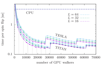
To single out the effect of hardware performance we measured the average spin-flip time in nanoseconds for both GPUs and the CPU. To this end, we ran the simulations for a range of different numbers of parallel walkers for a fixed number of attempted spin flips, starting out from the known perfect multicanonical weights as derived from the density of states [43]. Time measurements were only taken after the equilibration phase. The results for systems of linear sizes $L=16$, $L=32$, and $L=64$ are shown in Fig. 2. Due to the parallelism being only between walkers and not through domain decomposition of single spin lattices, the results are only weakly dependent on system size, the effect being mostly related to the changing degree of locality of memory accesses in incrementing the energy histograms. As expected, we find somewhat smaller times for the Titan card with higher clock frequency. Note, however, that this card performs dynamic frequency scaling in a window below the maximum clock frequency to automatically control the temperature and power consumption. To more clearly exhibit the algorithmic effects, we added a few seconds of sleep after producing each data point, thus preventing the card from clocking down.

The general trend of decreasing spin-flip times as the number of walkers is increased is an effect of the latency hiding approach discussed above that leads to generally improved performance as the cards are overloaded beyond the physical number of cores. There is a hierarchy of two levels of steps in the data which are connected to the commensurability of the loads to the available resources. One block of 256 threads per SMX corresponds to 3328 threads for the Tesla K20m with 13 SMX and 3840 threads for the Titan with 15 SMX. For any walker numbers in between these steps, the SMX are unevenly loaded, leading to sub-optimal performance. The larger-scale steps occur when the maximum number of eight resident 256-thread blocks per SMX is reached, corresponding to $N_{\mathrm{opt}}=8\times 3328=26\,624$ and $N_{\mathrm{opt}}=8\times 3840=30\,720$ threads for the Tesla K20m and Titan Black, respectively. Beyond these optima, the surplus blocks need to run in a separate round, again at sub-optimal uneven load of the SMX. We use these observations to automatically set the number of walkers to be at the first and lowest minimum if the user does not provide $W$ explicitly. This can be achieved using the kernel directive __launch_bounds__.

The straight line in Fig. 2 is the reference time for our CPU node, run with 24 threads on the dual Xeon nodes, which comes in at about $3.3\text{\,}\mathrm{n}\mathrm{s}$, practically independent of system size. The optimal spin-flip times of $0.22\text{\,}\mathrm{n}\mathrm{s}0.27\text{\,}\mathrm{n}\mathrm{s}$ for the Tesla K20m and $0.16\text{\,}\mathrm{n}\mathrm{s}0.17\text{\,}\mathrm{n}\mathrm{s}$ for the Titan Black result in effective hardware speedup factors up to $15$ and $21$, respectively. Note that in this performance comparison we use a whole CPU node with 12 cores as the reference. In the customary comparison to a single CPU core, these numbers thus would have to be multiplied by a factor of 12, resulting in speedups of 180 and 252, respectively. The factor of $1.4\text{\,}1.6\text{\,}$ between the two GPUs is compatible with the ratio of the specified peak performances of the cards as indicated in Table 1 and is a result of the larger number of SMX units and increased clock frequency of the Titan Black card as compared to the Tesla K20m.

3.2 Software performance

Figure 3: Average number of iterations until convergence for the parallel multicanonical method on GPU as a function of the number of walkers. The dashed lines indicate the number of iterations for the CPU (24 walkers) for the three different system sizes. Note that the number of iterations only depends on the number of walkers and the RNG seeds and hence is identical for runs on both GPUs.

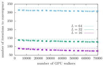
We proceed with the algorithmic or software performance. To capture it, we investigated the number of weight iterations required and the resulting total GPU computing time until convergence as a function of the number of GPU walkers in steps of the block size $256$. The number of iterations in this process is in itself a random variable, and hence to derive meaningful results we averaged over $32$ independent runs performed with different RNG seeds. Error bars were obtained from the fluctuations of the measurements. The parallelization employed here is via independent copies of the system that all contribute to the sampling of the same probability distribution. If in equilibrium, the independence of the copies should improve the estimate due to a reduction in autocorrelations as compared to a purely sequential process.

As outlined above, we employ an equilibration phase of $N_{\mathrm{therm}}\propto w$ updates (with width $w=L^{2}+1$ for the full energy range) at the beginning of each iteration. This is a compromise in that it is not necessarily enough to sufficiently equilibrate. As the number of walkers is increased, the number of histogram samples $N_{\mathrm{updates}}$ is reduced according to Eq. (7), such that the proportion of time spent on equilibration increases with $W$. As a result, it is seen from our results summarized in Fig. 3 that the required number of iterations mildly decreases with $W$ and seemingly settles. The behavior of the required number of iterations depends significantly on the number $N_{\mathrm{therm}}$ of equilibration updates, and for shorter thermalization phases the required number of iterations is found to increase with $W$ (not shown). As expected, the number of iterations increases with the system size $L$ as this increases the range of possible energy values to be covered by the walkers.

Figure 4: Average simulation time until convergence for the parallel multicanonical method on two different GPUs (crosses: Tesla K20m, circles: Titan Black) as a function of the number of walkers. The horizontal lines show the times obtained with the identical algorithm on one CPU node (24 threads using hyper-threading). Vertical dashed lines indicate the optimal occupancy as derived from Fig. 2.

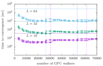
The total GPU computing time as a function of the number of GPU walkers is shown in Fig. 4. Horizontal lines indicate the average computation times on 12 CPU cores (24 threads with hyper-threading). As expected, the total simulation time clearly increases with system size. The GPU simulations finish in shorter time in the full range of cases considered. Comparing the two different GPU environments considered, we find that again the Titan Black card is consistently faster than the Tesla K20m, as expected from the hardware specifications. The marked minima in the total computational time indicated by vertical dashed lines coincide with the minima in the hardware times shown in Fig. 2 and are hence a result of the optimal load of the cards achieved there. Although in some cases the higher-order minima are not significantly worse than the first one, we recommend using the first optimum as automatically chosen by our code, which can also be easily calculated manually in the CUDA Occupancy Calculator spreadsheet as the product of “total number of multiprocessors” and “maximal threads per multiprocessor”.

Figure 5: Estimated speedup, i.e., reduction in wall-clock time required until convergence, for the parallel multicanonical method on different GPUs (Tesla K20m, Titan Black) as a function of the number of walkers. Vertical dashed lines indicate the optimal occupancies. The speedup is obtained compared to reference times from simulations on one CPU node (24 threads with hyper-threading). Data points mark the median speedup and the shaded areas indicate the confidence interval including $2/3$ of the data.

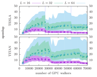
Comparing the computational time to convergence for runs on GPU and CPU we can derive a speedup factor, which is shown in Fig. 5. The average speedup is achieved at the point of optimal occupancy and works out at around $20$ and $25$ for the Tesla K20m and Titan Black cards, respectively. The relative size of these speedups is again compatible with the relative peak performance of these devices. These speedups are slightly larger than those found for the spin-flip times (which were 15 and 21 for the K20m and Titan Black, respectively), which is an effect of the slight decrease in the number of iterations with $W$ shown in Fig. 3. From an environmental perspective this means that if the CPU node requires $2\times$95\text{\,}\mathrm{W}$=$190\text{\,}\mathrm{W}$$ for a given task, the Tesla K20m and Titan Black GPUs would achieve compatible results for $11.3\text{\,}\mathrm{W}$ and $10.0\text{\,}\mathrm{W}$, respectively, according to their thermal design power as indicated in Table 1. Note, however, that this does not take into account the power consumption of the host CPU system in case of the GPUs as well as the power consumption of components other than the CPU itself in the CPU node.

Figure 6: Estimated algorithmic speedup, i.e., ratio of the total number of updates per walker (including thermalization) until convergence for a simulation with $24$ threads (corresponding to the CPU code) and a run with $W$ threads on the Titan Black GPU. Without statistical gain from independent walkers, the optimal ratio is $N_{24}/N_{W}=W/24$ indicated by the dashed black line. Data points mark the median speedup and the shaded areas indicate the confidence interval including $2/3$ of the data.Vertical dashed lines indicate the optimal occupancies.

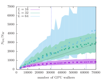
We can go one step further and consider a hardware-independent algorithmic speedup by considering the ratio of the total number of updates (including thermalization) performed per walker until convergence between the CPU and GPU implementations [10]. Figure 6 shows the corresponding strong scaling plot for the Titan Black GPU. The optimal scaling, where each doubling of threads results in a reduction of number of updates by a factor of two, is indicated by the dashed line. We note that for intermediate values of $W$ we observe a super-linear speedup that is an effect of the increased statistical independence of the parallel walkers as compared to the serial run. For very large numbers of walkers, on the other hand, we eventually expect an only sub-linear speedup due to the time spent in thermalization. This effect is only clearly seen for $L=16$, however, while for $L=32$ it just sets in at the edge of the range of $W$ considered here, and it is not visible for $L=64$. For larger system sizes we expect the onset of this effect to be shifted further towards larger numbers of parallel walkers. This clearly indicates that for usual system sizes the method is efficiently applicable for computations on massively parallel machines with many tens of thousands of cores.

3.3 Verification of physical results

To demonstrate the correctness and proper convergence of the method, we compare the final estimate of the density of states resulting from a production run with fixed weights to the known exact result [43]. The estimate of the density of states is obtained from a final production run with a total runtime of $1\text{\,}\mathrm{h}$. Here, we restricted ourselves to the Titan GPU card with $30\,720$ GPU walkers, which is the theoretically optimal choice as discussed above. We use the function of the code that is employed for the weight iterations also in the production run, with the only difference that the resulting histogram is not used to define new weights. To allow for the estimation of statistical errors, we divide the total number of attempted spin flips into $100$ individual calls to the multicanonical simulation function and use the resulting individual histograms to determine error bars from a jackknife analysis [46]. Thus, a single simulation with parallel walkers allows us to determine an estimate of the density of states and an estimate of the error for each energy bin. The result is shown in Fig. 7. As seen in the main panel, there is excellent agreement of the estimate $\overline{\ln\Omega}(E)$, shown in dashed colored lines with occasional error bars, to the exact result $\ln\Omega(E)$, shown as black lines. In order to fix the overall normalization, we ensure that the total number of states represented by $\exp[\overline{\ln\Omega}(E)]$ is $2^{L^{2}}$. All calculations are directly performed for the logarithm of $\Omega$ to avoid numerical overflows. As a result, the error bars shown are errors of the logarithm of the density of states.

Figure 7: Estimate of the logarithm of the density of states of the 2D Ising model from massively parallel multicanonical simulations on the Titan GPU card with $30\,720$ walkers and a fixed runtime of one hour a final production run performed for several system sizes. The solid lines show the exact solution according to Ref. [43], which agrees well with the estimates within error bars. The inset shows the jackknife errors, $\epsilon=\epsilon(\overline{\ln\Omega}(E))$, as dashed lines and absolute deviations from the exact solution, $\Delta=|\overline{\ln\Omega}(E)-\ln\Omega(E)|$, as solid lines.

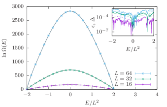
A more detailed quantitative comparison is provided by the absolute deviation from the exact result, $\Delta=|\overline{\ln\Omega}(E)-\ln\Omega(E)|$, in comparison to the jackknife error, $\epsilon=\epsilon(\overline{\ln\Omega}(E))$, as shown in the inset of Fig. 7. We observe the best agreement, i.e., the smallest deviation, around the center of the energy range. Here also the statistical error is smallest. This is a natural consequence of the vastly larger number of available states around $E=0$ as compared to the case of very large or very small energies. The ground state, for instance is only twofold degenerate. These observations notwithstanding, the statistical accuracy observed is very good and it can be systematically improved by using even more statistics in the production run. In general, we recommend to use the multicanonical weights to sample the quantities of interest in a production run. This guarantees a known exponential convergence behavior to equilibrium and allows for the reliable estimation of statistical errors. This is in contrast to the approach of using the estimated weights and density of states directly to estimate quantities such as the average energy and specific heat, where the analysis of systematic and statistical errors is much more difficult. We repeated the production run also for the Tesla K20m with $26\,624$ walkers and a full CPU compute node with $24$ walkers. We define the average statistical gain as the ratio between the squared statistical errors estimated for the density of states, $\epsilon^{2}_{\rm cpu}/\epsilon^{2}_{\rm gpu}$. We find average statistical gains of about $17$ and $23$ for the Tesla K20m and the Titan Black cards, respectively, which are consistent with the speedups found before for the weight iteration.

4 Conclusions

We demonstrated the suitability of parallel multicanonical simulations for massively parallel architectures. As a test platform we considered graphics cards, which play an increasingly important role in high-performance computing at all scales, in particular due to their favorable relation of performance to price and power consumption. To be representative of typical installations accessible to users, we used two Nvidia GPUs, one from the consumer series (GTX Titan Black) and one professional computing card (Tesla K20m). In comparison to a full CPU node with 12 cores (and using 24 hyper-threads) we find a significant speedup if the card is sufficiently occupied, with a median of around 25 for the GTX Titan Black and 20 for the Tesla K20m GPU. For the perhaps more standard comparison to a single CPU core these speedups need to be multiplied by a factor of 12, resulting in improvement factors of 300 and 240, respectively. Such speedups exceed the improvement expected from the measured hardware performance, which is the result of an additional algorithmic advantage due to the statistical independence of the walkers. This effect is also reflected in a reduction of the number of required updates until convergence. The physical result, namely an equilibrium estimate of the density of states, is found to be in statistical agreement with the exact solution up to high precision.

An efficient parallelization of Markov chain approaches is ultimately limited by the need to equilibrate each parallel walker, since the thermalization itself cannot be parallelized. For the present implementation of parallel multicanonical simulations applied to at least 1000 spins, however, we find that this effect sets in only beyond the maximum number of 70 000 threads studied here. For realistic system sizes we hence expect good scaling up to at least $10^{5}$ cores, demonstrating that such schemes are applicable for calculations on the largest computational resources available, including non-GPU hardware such as BlueGene/Q, Cray, or other massively parallel compute cluster architectures.

Appendix A Measures of Convergence

Figure 1: Effect of the number of thermalization sweeps $f_{\rm therm}$ on the convergence of the multicanonical iteration (Tesla K20m, $W=26\,624$) measured with the Kullback-Leibler divergence (top) or the Chebyshev distance (bottom) for an $L=32$ system. The strong oscillations for small numbers of thermalization updates may be attributed to non-equilibrium artifacts which are carried along in the weight estimation.

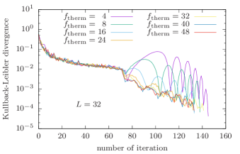
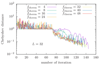
In Fig. 1 we present exemplary results from the multicanonical weight iteration on the Tesla K20m card with $W=26\,624$ walkers showing two different quantities used to assess convergence. The protocol used is described above in Sec. 3, using an initial thermalization phase of $N_{\rm therm}=f_{\rm therm}w$ attempted spin flips followed by $N_{\mathrm{updates}}$ updates to the histograms. According to (7) $N_{\mathrm{updates}}$ is systematically increased once $w=L^{2}+1$ by multiplying it by a factor $1.1$ after each iteration. The Kullback-Leibler divergence is defined in Eq. (6) and once this measure falls below $10^{-4}$ the simulation aborts. In addition, we show the Chebyshev distance $d_{c}$ defined as the maximal deviation of the histogram $H(x)$ from the expected value of a flat distribution, $m=N_{\rm updates}/N_{\rm bins}$

$$d_{c}=\max_{x}(|H(x)/m-1|).$$ (8)

This is closely related to common measures of a maximal deviation from the mean in the context of generalized-ensemble methods. The initial lower bound $d_{c}\geq 1$ observed from the lower panel of Fig. 1 is a result of almost empty histogram bins with $H(x)\approx 0$. From the data shown it is apparent that a convergence criterion $d_{c}<d_{c,\mathrm{flat}}=0.05$ for the Chebyshev distance would lead to a stopping time comparable to that resulting from the Kullback-Leibler criterion.

Both measures are quite sensitive to the behavior at the boundaries of the energy range discovered at any given time and the effect of empty bins. Note, however, that the Kullback-Leibler divergence automatically assigns zero weight to such bins. After the full range of energies has been discovered (here around 70 iterations), the number of updates $N_{\rm updates}$ is increased by a factor of $1.1$ in each iteration, leading to a pronounced change of behavior of the development of the convergence metrics at this point. We notice rather strong oscillations in $d_{k}$ and $d_{c}$ for short thermalization times, which we attribute to the presence of non-equilibrium artefacts in the recorded histograms, leading to distorted weight functions for the following iterations. These are carried over to successive iterations by the weight update and for low statistics per walker they may take a long time to be corrected. In fact, one can easily imagine that a sufficiently strong correction in the weights would require a sizable subset of walkers to transit out of (or into) now less favorable (more favorable) regimes. If the short thermalization pass does not allow for this to happen, the next iteration records again too many (or too few) signals in these regimes, leading to even stronger weight distortion. This explains the oscillatory behavior.

We note that from general random-walk arguments, one might deduce a scaling of $N_{\rm therm}\propto w^{z}$, but we found such a prescription to devote too much time to thermalization. Hence, we chose the heuristic approach with $N_{\rm therm}=f_{\rm therm}w$ and tuned $f_{\rm therm}$ to minimize oscillations. It is clear that this tuning leads to model specific parameters, and for optimal performance it would need to be repeated for different models to be considered.

References

- [1] G.E. Moore, Electronics 38 (1965) 114.
- [2] M. McCool, J. Reinders, A. Robison, Structured Parallel Programming: Patterns for Efficient Computation, Morgan Kaufman, Waltham, MA, 2012.
- [3] M. Weigel, Phys. Rev. E 84 (2011) 036709.
- [4] K. Hukushima, K. Nemoto, J. Phys. Soc. Jpn. 65 (1996) 1604.
- [5] B.A. Berg, T. Neuhaus, Phys. Lett. B 267 (1991) 249; Phys. Rev. Lett. 68 (1992) 9.
- [6] W. Janke, Int. J. Mod. Phys. C 03 (1992) 1137; Physica A 254 (1998) 164; Histograms and All That, in: Computer Simulations of Surfaces and Interfaces, NATO Science Series, Vol. 114, edited by B. Dünweg, D.P. Landau, and A.I. Milchev, Kluwer, Dordrecht, 2003, pp. 137–157; and in: Computational Many-Particle Physics, edited by H. Fehske, R. Schneider, and A. Weiße, Lect. Notes Phys. 739, Springer, Berlin, 2008, pp. 79-140.
- [7] F. Wang, D.P. Landau, Phys. Rev. Lett. 86 (2001) 2050; Phys. Rev. E 64 (2001) 056101.
- [8] B.J. Schulz, K. Binder, M. Müller, D.P. Landau, Phys. Rev. E 67 (2003) 067102.
- [9] M. Weigel, T. Yavors’kii, Physics Procedia 15 (2011) 92.
- [10] J. Zierenberg, M. Marenz, W. Janke, Comput. Phys. Commun. 184 (2013) 1155; Physics Procedia 53 (2014) 55.
- [11] T. Vogel, Y.W. Li, T. Wüst, D.P. Landau, Phys. Rev. Lett. 110 (2013) 210603.
- [12] J.D. Owens, M. Houston, D. Luebke, S. Green, J.E. Stone, J.C. Phillips, in: Proceedings of the IEEE, Institute of Electrical and Electronics Engineers, New York, 2008, p. 879.
- [13] M. Weigel, A. Arnold, P. Virnau (eds.), Computer Simulations on Graphics Processing Units, Eur. Phys. J. – Special Topics 210, Springer, Heidelberg, 2012.
- [14] B. Block, P. Virnau, T. Preis, Comp. Phys. Commun. 181 (2010) 1549.
- [15] M. Weigel, Comput. Phys. Commun. 182 (2011) 1833.
- [16] M. Weigel, J. Comp. Phys. 231 (2012) 3064.
- [17] M. Lulli, M. Bernaschi, G. Parisi, Comput. Phys. Commun. 196 (2015) 290.
- [18] C.A. Navarro, W. Huang, Y. Deng, Comput. Phys. Commun. 205 (2016) 48.
- [19] J. Gross, W. Janke, M. Bachmann, Comput. Phys. Commun. 182 (2011) 1638; Physics Procedia 15 (2011) 29.
- [20] J. Zierenberg, N.G. Fytas, W. Janke, Phys. Rev. E 91 (2015) 032126.
- [21] W. Janke, S. Kappler, Phys. Rev. Lett. 74 (1995) 212.
- [22] M. Weigel, Physics Procedia 3 (2010) 1499.
- [23] B.A. Berg, W. Janke, Phys. Rev. Lett. 80 (1998) 4771.
- [24] S. Schöbl, J. Zierenberg, W. Janke, Phys. Rev. E 84 (2011) 051805.
- [25] T. Sugihara, J. Higo, H. Nakamura, J. Phys. Soc. Jpn. 78 (2009) 074003.
- [26] V.V. Slavin, Low Temp. Phys. 36 (2010) 243.
- [27] A. Ghazisaeidi, F. Vacondio, L.A. Rusch, J. Lightwave Technol. 28 (2010) 79.
- [28] J. Zierenberg, N.G. Fytas, M. Weigel, W. Janke, A. Malakis, Eur. Phys. J. – Special Topics 226 (2017) 789.
- [29] J. Zierenberg, M. Wiedenmann, W. Janke, J. Phys: Conf. Ser. 510 (2014) 012017.
- [30] J. Zierenberg, W. Janke, Phys. Rev. E 92 (2015) 012134.
- [31] A. Nußbaumer, J. Zierenberg, E. Bittner, W. Janke, J. Phys.: Conf. Ser. 759, (2016) 012009.
- [32] J. Zierenberg, P. Schierz, W. Janke, Nat. Commun. 8 (2017) 14546.
- [33] J. Zierenberg, M. Mueller, P. Schierz, M. Marenz, W. Janke, J. Chem. Phys. 141 (2014) 114908.
- [34] J. Zierenberg, W. Janke, Europhys. Lett. 109 (2015) 28002.
- [35] J. Zierenberg, K. Tholen, W. Janke, Eur. Phys. J. – Special Topics 226 (2017) 683.
- [36] M. Marenz, W. Janke, Phys. Rev. Lett. 116 (2016) 128301.
- [37] K. Austin, J. Zierenberg, W. Janke, Macromolecules 50 (2017) 4054.
- [38] A.M. Ferrenberg, D.P. Landau, Y.J. Wong, Phys. Rev. Lett. 69 (1992) 3382.
- [39] M. Manssen, M. Weigel, A.K. Hartmann, Eur. Phys. J. Special Topics 210 (2012) 53.
- [40] L.Yu. Barash, L.N. Shchur, Comput. Phys. Commun. 185 (2014) 1343.
- [41] J.K. Salmon, M.A. Moraes, R.O. Dror, D.E. Shaw, in: Proceedings of 2011 International Conference for High Performance Computing, Networking, Storage and Analysis, ACM, New York, 2011.
- [42] B.M. McCoy, T.T. Wu, The Two-Dimensional Ising Model, Harvard University Press, Cambridge, 1973.
- [43] P.D. Beale, Phys. Rev. Lett. 76 (1996) 78.
- [44] S. Kullback, R.A. Leibler, Ann. Math. Stat. 22 (1951) 79.
- [45] W. Janke, B.A. Berg, M. Katoot, Nucl. Phys. B 382 (1992) 649.
- [46] B. Efron, The Jackknife, the Bootstrap and Other Resampling Plans, Society for Industrial and Applied Mathematics [SIAM], Philadelphia, 1982.