Aspects of the modified regularized long-wave equation

F. ter Braak^† and W. J. Zakrzewski^††

Department of Mathematical Sciences,
University of Durham, Durham DH1 3LE, U.K.

^(†) floris.ter-braak@durham.ac.uk
^(††) w.j.zakrzewski@durham.ac.uk

We study various properties of the soliton solutions of the modified regularized long-wave equation. This model possesses exact one- and two-soliton solutions but no other solutions are known. We show that numerical three-soliton configurations, for which the initial conditions were taken in the form of a linear superposition of three single-soliton solutions, evolve in time as three-soliton solutions of the model and in their scatterings each individual soliton experiences a total phase-shift that is the sum of pairwise phase-shifts. We also investigate the soliton resolution conjecture for this equation, and find that individual soliton-like lumps initially evolve very much like lumps for integrable models but eventually (at least) some blow-up, suggesting basic instability of the model.

1 Introduction

Integrable partial differential equations in $(1+1)$ dimensions, such as the KdV and the non-linear Schrödinger equation, possess infinitely many conservation laws which implies that such systems possess soliton solutions; these solitons are localised waves which preserve their shape and velocity before and after the scattering, but they do experience a phase-shift as a result of the scattering [5]. However, integrable models are quite rare, and some physical events can be described by models which possess soliton-like structures (such as general vortices, skyrmions and baby skyrmions) but are not integrable. Furthermore, the scattering properties of their soliton-like solutions are often not that different, in the sense that the amount of emitted radiation is not very large. Therefore, these models can loosely be described as ‘almost-integrable’. This has lead to various attempts to define the concept of quasi-integrability (see, e.g., paper [2] and references therein). Attempts have also been made to relate this concept to the extra (very special) symmetries satisfied by the two-soliton solutions [3].

In fact, the whole concept of integrability can be defined in various ways [8]. One of such definitions is Hirota integrability, which is based on Hirota’s method for obtaining multi-soliton solutions of non-linear models (and we will, when it is important to stress this fact, refer to them as Hirota solutions). In addition, it is often claimed that if this method leads to the construction of the exact one-, two- and three-soliton Hirota solutions, the model is considered to be Hirota integrable [7]. On the other hand, partial differential equations which only possess one- and two-soliton solutions, also known as partial integrable models, are not Hirota integrable [5]. (Note that this does not necessarily mean that solutions describing three or more solitons do not exist for these models; it only shows that they cannot be obtained using the Hirota method.) One of such models is the modified regularized long-wave (mRLW) equation, which we discuss in detail in this paper.

It has also been observed that if a set of equations is Hirota integrable, they satisfy the more conventional definitions of integrability [6]. Thus it is interesting to try to better understand why, whereas models with only one- and two-soliton Hirota solutions do not appear to satisfy the conventional definitions of integrability, systems which also possesses three-soliton Hirota solutions do satisfy the conventional definitions of integrability. This raises the question: what is so special about three-soliton Hirota solutions?

In this paper we look in detail at various (numerical) properties of the mRLW equation. In the next section we recall this equation and the exact form of its one- and two-soliton solutions. Then we compare the analytical two-soliton scattering with our numerical approximation in order to test the accuracy and stability of our finite difference scheme. We also check whether the numerically evolved linear superposition of two single-soliton solutions is a good approximation to the corresponding analytical two-soliton solution, because we want to use a linear superposition of three single-soliton solutions as the initial conditions for our numerical three-soliton simulations. We find that this approach gives us essentially the same results as the ones obtained by using the exact two-soliton solutions. In section 3 we investigate the time evolution of three-soliton systems obtained in such a way and look at the phase-shifts experienced by these solitons during their interactions. Finally, in section 4 we look at some simulations using lumps (i.e., functions which do not solve the mRLW equation) in order to test the soliton resolution conjecture. The last section of the paper presents our conclusions and plans for future work.

A large part of our results is based on numerical simulations of the mRLW equation. Since we used a numerical procedure which combined explicit and implicit finite difference methods, the work involved the discretisation in both time and space, and so had large memory requirements. Most of the simulations involved grid-spacing of $h=0.1$ and time-steps of $\tau=0.001$. To assess the reliability of our procedures we have altered these values and we are confident that the results presented in the paper are correct. Since our procedure is second order in time, we require an analytic expressions of the fields at the first $2$ time levels. We took them from the expressions of $q(x,t)$ given in the paper and refer to as ‘initial conditions’. The spatial boundary conditions were fixed. More details on the numerical procedure are presented in appendix A.1, and the particular values of various parameters used in the reported simulations are gathered in a table in appendix A.2.

2 The modified regularized long-wave equation

The mRLW equation, introduced by J. D. Gibbon, J. C. Eilbeck and R. K. Dodd [4], is defined by

$$q_{xxtt}+2q_{xx}q_{tt}+4q_{xt}^{2}-q_{xt}-q_{tt}=0\,,$$ (1)

where $q=q(x,t)$ is a real-valued function, and the subscripts $x$ and $t$ denote partial differentiation with respect to these variables. It is known that this equation possesses analytical one- and two-soliton Hirota solutions [4], where the one-soliton solutions are given by

$$q=\ln\left(1+e^{\eta_{1}}\right)$$ (2)

and the two-soliton solutions take the form

$$q=\ln\left(1+e^{\eta_{1}}+e^{\eta_{2}}+A_{12}e^{\eta_{1}+\eta_{2}}\right)\,,$$ (3)

where

$$\eta_{i}=k_{i}x-\omega_{i}t+\delta_{i}\,,\quad i=1,2\,,$$ (4)

and

$$A_{12}=-\frac{(\omega_{1}-\omega_{2})^{2}(k_{1}-k_{2})^{2}+(\omega_{1}-\omega_{2})(k_{1}-k_{2})-(\omega_{1}-\omega_{2})^{2}}{(\omega_{1}+\omega_{2})^{2}(k_{1}+k_{2})^{2}+(\omega_{1}+\omega_{2})(k_{1}+k_{2})-(\omega_{1}+\omega_{2})^{2}}\,.$$ (5)

In these expressions, the parameters $k_{i}$ and $\omega_{i}$ are constrained by the following dispersion relation

$$\omega_{i}=\frac{k_{i}}{1-k_{i}^{2}}\,,\quad i=1,2\,.$$ (6)

The actual soliton fields of Gibbon et al. are defined by $u\equiv-q_{xt}$.

In what follows, for definiteness, we consider only $1>k_{1}>k_{2}>0$. This implies that both the amplitude and velocity of each soliton will be positive. Furthermore, the soliton corresponding to $\eta_{1}$ will have a larger amplitude and velocity than the soliton corresponding to $\eta_{2}$. To illustrate this, in figure 1 the red lines present the plots of the spatial dependence of $u$ at various values of $t$ of an analytical two-soliton simulation. The other curves will be discussed below.

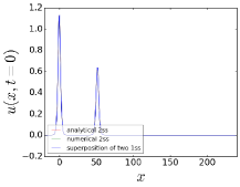
(a) At $t=0$

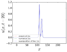
(b) At $t=20$

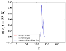
(c) At $t=22.5$

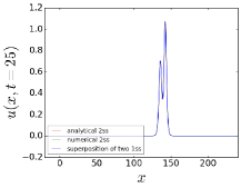
(d) At $t=25$

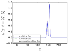
(e) At $t=27.5$

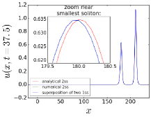
(f) At $t=37.5$

Figure 1: This figure shows two solitons interacting with each other at different points in time for three simulations. The red line is obtained using the analytic expression given by equation (3), the green line shows the numerical time evolution of equation (3) as initial conditions, and the blue line shows the numerical time evolution of equation (7) as initial conditions. (Note that the three simulations are so close that their plots are barely distinguishable with the naked eye.)

The Hirota method does not generate three-soliton solutions for the mRLW equation, which implies that the model is not Hirota integrable. Furthermore, to our knowledge, nobody has found an analytic expression describing three or more solitons (using any method). Thus, we need to use numerical methods (see the appendix for more details) in order to study the time evolution of three-soliton configurations. To test this scheme empirically, we have used the initial field configurations (i.e., the initial conditions) expressed by equation (3) and evolved the configuration in time using our procedures. The green lines in figure 1 shows the plots for such a simulation which is produced using the same values for the angular frequencies $\omega_{i}$ and phase constants $\delta_{i}$ as for the aforementioned analytical simulation (see appendix A.2 for more information). This allows us to compare the numerical solution with the analytical results. Since these two lines in figure 1 are so close to each other that one can hardly distinguish them, the numerical solution is a good approximation of the analytical values.

Furthermore, it will be useful for the simulations discussed in the next section to also consider the time evolution of the following initial conditions

$$q=\ln\left(1+e^{\eta_{1}}\right)+\ln\left(1+e^{\eta_{2}}\right)\,.$$ (7)

The blue lines in figure 1 present the results of this evolution, where again the parameters governing $\eta_{1}$ and $\eta_{2}$ have exactly the same values as for the previously two discussed simulations. All together, figure 1 demonstrates that the numerical time evolution of a linear superposition of two exact one-soliton solutions produces results that are also almost indistinguishable from those of the analytical and numerical two-soliton simulations (provided that the two solitons are initially placed far apart from each other).

The above described three different simulations are so close that with the naked eye they are indistinguishable on the scale used in figure 1. Therefore, in order to illustrate how close the three lines are, in figure 1(f) we have added an insert of the region near the amplitude of the smallest soliton on a much smaller scale. This insert demonstrates very clearly that there is indeed a very small discrepancy between the analytical result and both the numerical simulations, but even on this scale we cannot distinguish between the numerical time evolution of equation (3) and equation (7) (and upon zooming in on the region of the larger soliton, we find that the discrepancies between the simulations are of similarily small magnitudes). This is expected since looking at the time evolution of the two solitons, we see that most of the interaction takes place when the solitons are close together. We see that in this case each soliton has a size of about $L\sim 20$, and since they are initially placed further apart than $L$ (see figure 1(a)), the errors of such an approximation are only in the interaction of their ‘tails’.

When the two solitons scatter, the only result of their interaction after the collision is the phase-shift they experience. In order to determine the analytical expression of this phase-shift, let us introduce two new variables $y\equiv x-\frac{\omega_{1}}{k_{1}}t$ and $z\equiv x-\frac{\omega_{2}}{k_{2}}t$. Then, substituting $y$ into $\eta_{1}$ and $\eta_{2}$ (i.e., $\eta_{1}=k_{1}y+\delta_{1}$ and $\eta_{2}=k_{2}(y+\frac{\omega_{1}}{k_{1}}t)-\omega_{2}t+\delta_{2}$ ) the exact two-soliton solution can be asymptotically approximated as

$$\lim_{t\to-\infty}u(y,t)\approx\frac{k_{1}\omega_{1}e^{\eta_{1}}}{\left(1+e^{\eta_{1}}\right)^{2}}\quad\text{and}\quad\lim_{t\to\infty}u(y,t)\approx\frac{k_{1}\omega_{1}e^{\eta_{1}+\ln A_{12}}}{\left(1+e^{\eta_{1}+\ln A_{12}}\right)^{2}}\,.$$ (8)

Similarly, introducing the variable $z$ gives

$$\lim_{t\to-\infty}u(z,t)\approx\frac{k_{2}\omega_{2}e^{\eta_{2}+\ln A_{12}}}{\left(1+e^{\eta_{2}+\ln A_{12}}\right)^{2}}\quad\text{and}\quad\lim_{t\to\infty}u(z,t)\approx\frac{k_{2}\omega_{2}e^{\eta_{2}}}{\left(1+e^{\eta_{2}}\right)^{2}}\,.$$ (9)

Thus, after the collision the solitary wave corresponding to $\eta_{1}$ is phase-shifted forward by $\ln A_{12}$ and the wave corresponding to $\eta_{2}$ is phase-shifted by $\ln A_{12}$ in the opposite direction.

In the following section we analyse the phase-shift that solitons experience during three-soliton scattering. Since no three-soliton solutions are known, we investigate them numerically, and so it will be useful to test the reliability of our numerical method for determining the phase-shifts of the analytical and numerical two-soliton simulations. We estimate this error by dividing the computationally observed phase-shift (from either the analytical or numerical simulation) by $\ln A_{12}$ (i.e., the analytical expression of the phase shift-shift). With this definition, we have found that the error is always small but it is somewhat sensitive to the details of our procedure. In fact we have found that in all our (analytical and numerical) simulations the error had always been smaller than $5.0\%$. Since we also observed errors close to $5.0\%$ for the analytical simulations, we can conclude that these errors are mainly a result of the algorithm of determining the phase-shift rather than resulting from the finite difference scheme approximating the mRLW equation.

Finally, let us briefly discuss the conserved charges for the mRLW equation. As far as we are aware, its only known conservation laws are given by

$$\partial_{t}\int\limits^{\infty}_{-\infty}\mathrm{d}x\;(-q_{xt})=\partial_{t}\int\limits^{\infty}_{-\infty}\mathrm{d}x\;u=0$$ (10)

and

$$\partial_{t}\int\limits^{\infty}_{-\infty}\mathrm{d}x\;(-q_{xx})=0\,,$$ (11)

which can be easily verified by taking the derivative of equation (1) with respect to $x$. Let us add that one can approximate the values of these conserved charges for the analytical one- and two-soliton solutions as follows

$$Q_{1}\equiv\int\limits^{\infty}_{-\infty}\mathrm{d}x\;(-q_{xt})=[-q_{t}]^{\infty}_{x=-\infty}\approx\sum\limits_{i=1}^{N}\omega_{i}\,,\quad N=1,2\,,$$ (12)

and

$$Q_{2}\equiv\int\limits^{\infty}_{-\infty}\mathrm{d}x\;(-q_{xx})=[-q_{x}]^{\infty}_{x=-\infty}\approx-\sum\limits_{i=1}^{N}k_{i}\,,\quad N=1,2\,.$$ (13)

In the next section, we check whether these quantities are also conserved for the numerically evolved three-soliton configurations.

3 Numerical three-soliton solutions

So far we discussed mainly two-soliton configurations. In this section we look at systems involving three solitons. As we stated before, the analytical three-soliton solutions (or solutions involving even more solitons) of the mRLW equation are not known, and they cannot be found by the Hirota method. This has been stated in literature and we have verified this claim for three and four solitons. So, we do not really know whether such solutions exist or not; all we know is that if they exist, their forms cannot be found by the Hirota method.

As we have shown in the previous section, a linear superposition of two single-soliton solutions is almost indistinguishable from the analytical two-soliton solution when, initially, these two solitons are far enough apart. Armed with this observation, we have numerically simulated the time evolution of a three-soliton system by using the linear superposition of three well-separated one-soliton solutions as the initial conditions for our simulations. In other words, we use

$$q=\ln\left(1+e^{\eta_{1}}\right)+\ln\left(1+e^{\eta_{2}}\right)+\ln\left(1+e^{\eta_{3}}\right)$$ (14)

to construct the initial conditions of a three-soliton system. We have performed many such simulations using a range of variables describing the frequencies of individual solitons and, in the next subsection, we discuss the results of two of such simulations for illustrative purposes.

3.1 Three-soliton interactions

We are primarily interested in three-soliton interactions, and so for the simulations discussed in this section the phase constants $\delta_{i}$ have always been chosen in such a way that all three solitons scatter with each other at more or less the same time. To illustrate this, figures 2

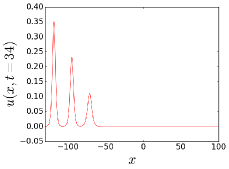
(a) At $t=34$

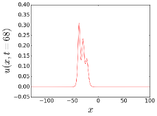
(b) At $t=68$

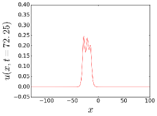
(c) At $t=72.25$

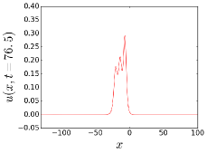
(d) At $t=76.5$

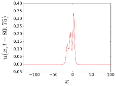
(e) At $t=80.75$

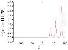
(f) At $t=114.75$

Figure 2: This figure shows three solitons interacting with each other at various points in time. Note that at all times during the interaction, there are three distinct maxima present.

and 4 show two of such interactions, where both simulations start at $t=0$ with the solitons placed far apart of each other.

For these two simulations, figures 3

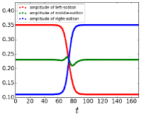
(a)

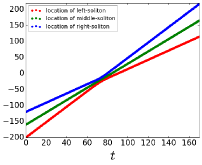
(b)

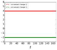
(c)

Figure 3: For figures 3(a) and 3(b), the red dots present the time dependence of the amplitude and the location of the left-soliton of the simulation shown in figure 2. Similarly, the green and blue dots correspond to the middle- and right-soliton, respectively. Finally, figure 3(c) shows how the conserved charges of the corresponding simulation vary with time.

and 5

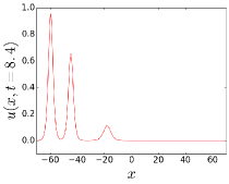
(a) At $t=8.4$

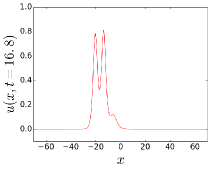
(b) At $t=16.8$

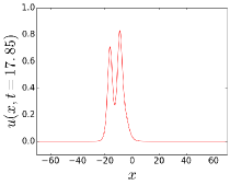
(c) At $t=17.85$

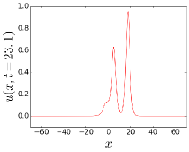
(d) At $t=23.1$

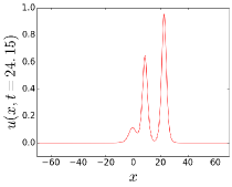
(e) At $t=24.15$

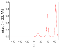
(f) At $t=32.55$

Figure 4: This figure shows three solitons interacting with each other at various points in time. Note that there is a small period of time ($17\lesssim t\lesssim 23$) during the collision where the smallest wave is ‘absorbed’ and there are only two distinct maxima present (see figure 4(c) for example).

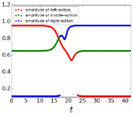
(a)

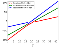
(b)

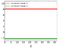
(c)

Figure 5: For figures 5(a) and 5(b), the red dots present the time dependence of the amplitude and the location of the left-soliton of the simulation shown in figure 4. Similarly, the green and blue dots correspond to the middle- and right-soliton, respectively. Finally, figure 5(c) shows how the conserved charges of the corresponding simulation vary with time.

show, respectively, the time dependence of the amplitude and the location (defined as the location of the amplitude of the wave) of each soliton, and the time dependence of the charges $Q_{1}$ and $Q_{2}$. Using these results, we have observed that for all our simulations, after the three-soliton interaction, the solitons recovered their original amplitudes and velocities with a numerical error of less than $0.1\%$. Furthermore, the quantities $Q_{1}$ and $Q_{2}$ have been incredibly well conserved for all our simulations with a numerical error of less than $0.001\%$ compared to the approximations given by equations (12) and (13). These results demonstrate that the solitons, in these configurations, behave as solitons in integrable models.

Assuming that the total phase-shift each soliton experiences when three solitons collide is the sum of the pairwise phase-shifts, then, analytically, we expect the location of the largest soliton (related to $\eta_{1}$) to experience a phase-shift forward by $\ln(A_{12})+\ln(A_{13})$, the soliton corresponding to $\eta_{2}$ to experience a phase-shift given by $-\ln(A_{12})+\ln(A_{23})$ and the smallest soliton to be phase-shifted by $-\ln(A_{13})-\ln(A_{23})$, where $A_{13}$ and $A_{23}$ are defined in a similar way as $A_{12}$ (see equation (5)). We found that the phase-shifts for all our simulations have always been within $5.0\%$ of the expected analytic value. Since these errors are consistent with the errors discussed near the end of section 2, we conclude that the phase-shifts experienced by each soliton during a numerical three-soliton interaction is additive, which suggest the non-existence of additional ‘three-body’ forces, (i.e., the phase shifts can be explained by the additivity of ‘two-body’ forces). This is another indicator that the solitons of our model behave like solitons in an integrable model.

4 Soliton resolution conjecture

In this section we investigate the time evolution of soliton-like lumps which are not analytical solutions of the mRLW equation. This is a test of the idea that such initial field configurations may eventually decouple into soliton-like and radiation-like components. For many non-linear dispersive equations there is evidence suggesting that such arbitrary finite-energy initial configurations always decouple in such a manner and this expectation is also referred to as the soliton resolution conjecture [10].

Of course the choice of the initial lump-like configuration is very arbitrary - one could take a Gaussian field or any other more complicated initial condition field for which the $u=-q_{xt}$ resembles a soliton-like structure. However, since our numerical scheme requires an analytical expression for $q$ and $q_{t}$ as initial conditions, and the field we are interested in is described by $u=-q_{xt}$, we are somewhat limited in our choices.

Figure 6

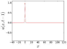
(a) At $t=1$

(b) At $t=1.4$

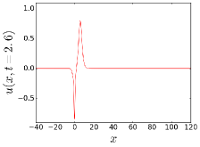
(c) At $t=2.6$

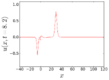
(d) At $t=8.2$

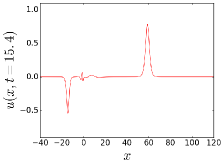
(e) At $t=15.4$

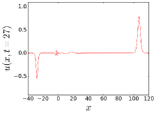
(f) At $t=27$

Figure 6: Plots of $x$-dependence of $u(x,t)$ (at various values of $t$) of the numerical evolution of $q$ field with the initial condition taken from equation (15).

shows the time evolution of our first choice of the lump given by

$$q=-t\tanh(x)\implies u=\operatorname{sech}^{2}(x)\,.$$ (15)

We started this simulation at $t=1$ and, as fig 6(a) shows, the initial conditions describe a lump with a positive amplitude located at $x=0$. Then figures 6(b) and 6(c) show that this initial configuration evolved into a lump and an anti-lump configuration. The anti-lump traveled to the left leaving behind some ‘radiation’, whereas the positive lump moved to the right without emitting any (visible) ‘radiation’ (see figures 6(d), 6(e), and 6(f)). The ‘radiation’ left behind by the anti-lump was also slowly moving to the left and (although it is difficult to see this by looking at figure 6) it also emitted some further ‘radiation’ which started to travel to the right (but not fast enough to catch up with the positive lump). We ran this simulation until $t=241$ without the system blowing up. The simulation might blow up if we run it for a longer time, but we lacked the computational power for studying this further. Let us add that when we repeated this simulation with a negative amplitude (i.e., using $u=-\operatorname{sech}^{2}(x)$ as initial conditions), then the simulation blew up at approximately $t=28.9$. From this we see that at least the ‘lump-like’ described by equation (15) was reasonably robust and long-lived.

However, this was not the case for the evolution of another ‘lump-like’ configuration, this time described by the following Gaussian function

$$q=-t\operatorname{erf}(0.5x)\implies u=\frac{1}{\sqrt{\pi}}\exp\left(-x^{2}\right)\,.$$ (16)

Its time evolution is presented in figure 7.

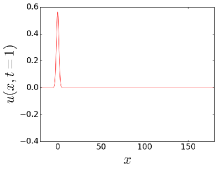
(a) At $t=1$

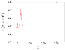
(b) At $t=6$

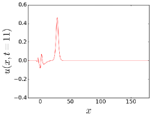
(c) At $t=11$

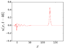
(d) At $t=46$

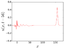
(e) At $t=56$

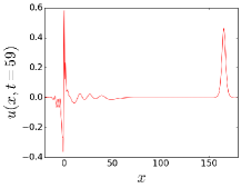
(f) At $t=59$

Figure 7: Plots of $x$-dependence of $u(x,t)$ (at various values of $t$) of the numerical evolution of $q$ field with the initial condition taken from equation (16).

This time we saw that the lump, which at the start of the simulation ($t=1$) was located at $x=0$ (see figure 7(a)), started to move to the right, also leaving some ‘radiation’ behind. However, our plots show that the ‘radiation’ started to develop larger amplitudes as the time progressed. This can be seen by comparing figure 7(e) with figure 7(f) which show that the amplitudes of the ‘radiation’ had grown significantly during a short period of time. In fact, at approximately $t=67.2$ the whole system blew up. The same happened when we repeated the simulation with a negative amplitude (i.e., using $u=-\pi^{-1/2}\exp\left(-x^{2}\right)$ as initial conditions). In this case the simulation blew up at approximately $t=11.9$ (i.e. again, smaller than for a positive initial amplitude of the lump).

Let us add that we believe that the blow-ups described in this section are not numerical artefacts, since we checked this by changing the parameters of the grid-spacing and time-steps, and they have always happened at roughly the same values of $t$.

So, to sum up, we feel that the blow-ups described in this section imply that the soliton resolution conjecture does not hold for the mRLW equation, whereas it does hold for many integrable systems such as the KdV and the non-linear Schrödinger equation. Numerically, this is the only observation we have found that distinguishes the non-integrable mRLW equation from many other integrable systems and this may be related to the fact that this model does not possess a conserved quantity which controls and limits the growth of the amplitude (such as the energy in many systems).

5 Conclusions and further comments

In this paper we have investigated the (numerical) time evolution of two- and three-soliton configurations of the mRLW equation. When we numerically evolved the initial conditions described by the analytic two-soliton solution and compared the results with the corresponding analytical simulation, we have found that they were essentially indistinguishable. This provided a good test of our numerical procedure and reassured us that the results of our simulations could be trusted. Furthermore, our results agreed with the results presented in the original paper by Gibbon et al. [4], where they overlapped. In addition to the investigation of the numerical two-soliton solutions, we have also studied the numerical time evolution of systems constructed by the superposition of two one-soliton solutions, and have found that these configurations approximated the analytical two-soliton solutions very closely.

This has led us to consider three-soliton configurations constructed by taking a superposition of three one-soliton solutions. The numerical time evolution of these three-soliton configurations behaved very much like those seen in integrable models; the field evolved well, there did not seem to be any breaking or changes to the individual solitons whenever they were far from each other, and after the scattering the solitons emerged with their original shapes and velocities. Furthermore, the phase-shift experienced by each soliton was additive, and the known conservation laws were also obeyed for such configurations. This suggests to us that analytical three-soliton solutions may exist (though their analytic forms cannot be found by Hirota’s method).

We also looked at the time evolutions of various lumps - i.e., fields that crudely resemble a single soliton field but are not exact solutions of the mRLW equation. We have found that the system blows up for some lumps, which is most likely a consequence of instabilities of the model which lead to the development of very steep gradients causing our numerical procedures to break down. We have checked that these blow-ups were genuine properties of the evolution of these field configurations rather than numerical artefacts. Our results imply that the soliton resolution conjecture does not hold for the mRLW equation. Numerically, this is the only property of this non-integrable model with a behaviour that differs from many other integrable models. It would therefore be interesting to study other systems which are not Hirota integrable but do possess one- and two-soliton Hirota solutions and check if such systems show similar properties to the mRLW equation (i.e., whether they possess numerical three-soliton solutions in which the solitons behave exactly as one would expect from integrable solitons, but the soliton resolution conjecture does not hold). This could shine some new light on the connection between (Hirota) integrability and the soliton resolution conjecture.

So overall, our results show that the mRLW model has many interesting properties and in many ways behaves like an integrable model. This has led us to consider whether we can think of this model as a finite perturbation of an integrable model and an obvious suggestion here is to think of this model as a perturbation of the KdV equation. So together with L. A. Ferreira we are now trying to carry out such a procedure and we hope that it will help us to understand the integrability/quasi-integrability properties of this model better. We hope to be able to say more on this topic soon.

Acknowledgements: We would like to thank L. A. Ferreira for many constructive and helpful comments and for working with us on some problems discussed in this paper. WJZ would like to thank the Royal Society for its grant to collaborate with L. A. Ferreira. Both authors thank the FAPESP/Durham University for their grant to facilitate their visits to the USP at São Carlos, and the Department of Physics in São Carlos for its hospitality.

Appendix A Numerical methods

Our numerical procedure for solving the mRLW equation combines the explicit and implicit methods of solving the equations of motion of the model. This is due to the fact that the term in the equation which contains the highest time derivatives also possesses spatial derivatives. A similar problem was encountered by J. C. Eilbeck and G. R. McGuire when they numerically investigated the regularized long-wave equation [1]. Their paper provides a detailed discussion of how to use such methods. We followed their ideas, modifying them appropriately for our investigations, and we present a short discussion of our procedure in the following subsection.

A.1 Numerical approximation of mRLW equation

First, to simplify the mRLW equation, we introduce a new field $p$ as follows

$$p=q_{t}$$ (17)

so that the mRLW equation takes the form

$$p_{xxt}+2q_{xx}p_{t}+4p_{x}^{2}-p_{x}-p_{t}=0\,.$$ (18)

We then take a finite set of points $x_{0},x_{1},\ldots,x_{N}$ and $t_{0},t_{1},\ldots,t_{K}$, and let $h$ denote the grid-spacing and $\tau$ the time-step. Furthermore, we denote the grid points as $(ih,m\tau)\equiv(i,m)$, where $i=0,1,2,\ldots,N$ and $m=0,1,2,\ldots,K$, and we employ the following notation: $p_{i}{}^{m}\equiv p(ih,m\tau)$ and $q_{i}{}^{m}\equiv q(ih,m\tau)$. Finally, we choose $v_{i}{}^{m}$ to denote our approximation to $p_{i}{}^{m}$, and $w_{i}{}^{m}$ to denote our approximation to $q_{i}{}^{m}$.

Next, we introduce the following central finite difference operators by their actions on $v_{i}{}^{m}$ as follows

$$\delta_{x}^{2}v_{i}{}^{m} =(v^{m}_{i+1}-2v_{i}{}^{m}+v^{m}_{i-1})/h^{2}\,,$$ (19)

$$H_{x}v_{i}{}^{m} =(v^{m}_{i+1}-v^{m}_{i-1})/2h\,,$$ (20)

$$H_{t}v_{i}{}^{m} =(v^{m+1}_{i}-v^{m-1}_{i})/2\tau\,,$$ (21)

and similarly on $w_{i}{}^{m}$. Applying these operators to equation (18) in a straightforward manner yields

$$\delta_{x}^{2}H_{t}v_{i}{}^{m}+2\delta_{x}^{2}w_{i}{}^{m}H_{t}v_{i}{}^{m}+4\left(H_{x}v_{i}{}^{m}\right)^{2}-H_{x}v_{i}{}^{m}-H_{t}v_{i}{}^{m}=0\,,$$ (22)

which can be rewritten as

$$\begin{split}-\frac{v_{i}^{m+1}}{2\tau}&+\frac{v_{i+1}^{m+1}-2v^{m+1}_{i}+v_{i-1}^{m+1}}{2h^{2}\tau}+\frac{w_{i+1}^{m}v_{i}^{m+1}-2w_{i}{}^{m}v_{i}^{m+1}+w^{m}_{i-1}v_{i}^{m+1}}{h^{2}\tau}\\ &=-\frac{v_{i}^{m-1}}{2\tau}+\frac{v_{i+1}^{m}-v_{i-1}^{m}}{2h}+\frac{v_{i+1}^{m-1}-2v_{i}^{m-1}+v_{i-1}^{m-1}}{2h^{2}\tau}\\ &\hskip 12.80373pt+\frac{w_{i+1}^{m}v_{i}{}^{m-1}-2w_{i}{}^{m}v_{i}^{m-1}+w_{i-1}^{m}v_{i}^{m-1}}{h^{2}\tau}\\ &\hskip 12.80373pt-\frac{(v_{i+1}^{m})^{2}-2v_{i+1}^{m}v_{i-1}^{m}+(v_{i-1}^{m})^{2}}{h^{2}}\,.\end{split}$$ (23)

Let us now introduce the following matrices

$$A\equiv\begin{pmatrix}1&0&0&\cdots&&0\\ \frac{1}{2h^{2}\tau}&a_{1}{}^{m}&\frac{1}{2h^{2}\tau}&0&&\vdots\\ 0&\frac{1}{2h^{2}\tau}&a_{2}{}^{m}&\frac{1}{2h^{2}\tau}&\\ \vdots&&\ddots&\ddots&\ddots&0\\ &&&\frac{1}{2h^{2}\tau}&a_{N-1}^{m}&\frac{1}{2h^{2}\tau}\\ 0&\cdots&&0&0&1\end{pmatrix}\,,$$ (24)

$$B\equiv\begin{pmatrix}v_{0}^{m+1}\\ v_{1}^{m+1}\\ v_{2}^{m+1}\\ \vdots\\ v_{N-1}^{m+1}\\ v_{N}^{m+1}\end{pmatrix}\,,\quad C\equiv\begin{pmatrix}c_{0}{}^{m}\\ c_{1}{}^{m}\\ c_{2}{}^{m}\\ \vdots\\ c_{N-1}^{m}\\ c_{N}^{m}\end{pmatrix}\,,$$ (25)

where

$$a_{i}{}^{m}\equiv\frac{-1+w_{i+1}^{m}-2w_{i}{}^{m}+w_{i-1}^{m}}{h^{2}\tau}-\frac{1}{2\tau}\,,$$ (26)

$$c_{0}{}^{m}\equiv v_{0}^{m+1}\,,\quad c_{N}^{m}\equiv v_{N}^{m+1}\,,$$ (27)

$$\begin{split}c_{i}{}^{m}\equiv&-\frac{v_{i}^{m-1}}{2\tau}+\frac{v_{i+1}^{m}-v_{i-1}^{m}}{2h}+\frac{v_{i+1}^{m-1}-2v_{i}^{m-1}+v_{i-1}^{m-1}}{2h^{2}\tau}\\ &+\frac{w_{i+1}^{m}v_{i}{}^{m-1}-2w_{i}{}^{m}v_{i}^{m-1}+w_{i-1}^{m}v_{i}^{m-1}}{h^{2}\tau}\\ &-\frac{(v_{i+1}^{m})^{2}-2v_{i+1}^{m}v_{i-1}^{m}+(v_{i-1}^{m})^{2}}{h^{2}}\,,\quad i=1,2,\ldots,N-1\,,\end{split}$$ (28)

so that equation (23) can be rewritten as the matrix equation

$$AB=C\,.$$ (29)

Hence, we need to solve this equation for the vector $B$. This can done by using the well-known $LU$ decomposition method [9].

Once we have solved for $B$, we have the values of $v_{i}^{m}$ at the next time level. One can then find the values of all $w_{i}^{m}$ by solving equation (17) using the central difference operator, that is,

$$v_{i}{}^{m}=\frac{w^{m+1}_{i}-w_{i}^{m-1}}{2\tau}\implies w_{i}^{m+1}=2\tau v_{i}{}^{m}+w_{i}^{m-1}\,.$$ (30)

We then repeat this procedure for all time levels in order to calculate the time evolution of any initial configuration.

It is not too difficult to verify that this scheme is both second-order accurate in $\tau$ and in $h$. Furthermore, we have extensively tested this scheme against the analytical one- and two-soliton solutions. These tests have shown that the numerical simulations approximate the analytical solutions extremely well without any (visible) loss of radiation. This indicates that, for the values of $h$ and $\tau$ that we have used, the scheme is stable and we can trust its results.

Finally, let us add that had we substituted the finite difference operators directly into the mRLW equation without first making the substitution expressed by equation (17), then the $4q_{xt}^{2}$ term would have yielded a term $(-w_{i+1}^{m+1}w_{i-1}^{m+1})/(2h^{2}\tau^{2})$; and since this term contains two unknowns, (i.e., $w_{i+1}^{m+1}$ and $w_{i-1}^{m+1}$), we would not have been able to solve for it. Moreover, for very similar reasons, we cannot use the well-known Crank-Nicolson method to numerically solve the mRLW equation.

A.2 Summary of parameters used to produce figures

Table 1 shows all the parameters used to produce the figures shown in this paper.

Table 1: This table summarizes the variables used on the simulations discussed in this paper and presented as plots in various figures.

	Figure 1	Figures 2 and 3	Figures 4 and 5	Figure 6	Figure 7
$x_{0}$	$-50$	$-220$	$-125$	$-600$	$-150$
$x_{N}$	$250$	$250$	$175$	$1200$	$350$
$h$	$0.1$	$0.1$	$0.1$	$0.1$	$0.1$
$t_{0}$	$0$	$0$	$0$	$1$	$1$
$t_{K}$	$40$	$170$	$42$	$241$	$81$
$\tau$	$0.001$	$0.001$	$0.001$	$0.01$	$0.001$
$\omega_{1}$	$5.00$	$0.80$	$0.80$	N/A	N/A
$\delta_{1}$	$0.00$	$66.51$	$16.63$	N/A	N/A
$\omega_{2}$	$3.00$	$1.33$	$3.07$	N/A	N/A
$\delta_{2}$	$0.00$	$110.90$	$63.77$	N/A	N/A
$\omega_{3}$	N/A	$1.84$	$4.28$	N/A	N/A
$\delta_{3}$	N/A	$152.88$	$89.00$	N/A	N/A

References

- [1] J. C. Eilbeck and G. R. McGuire, Numerical Study of the Regularized Longe-Wave Equation I: Numerical Methods, J. Comp. Phys., 19 1, 43-57 (1975)
- [2] L. A. Ferreira and W. J. Zakrzewski, The concept of quasi-integrability: a concrete example, JHEP, 1105 (2011)
- [3] L. A. Ferreira and W. J. Zakrzewski, Numerical and analytical tests of quasi-integrability in modified sine-Gordon models, JHEP, 58 (2014)
- [4] J. D. Gibbon, J. C. Eilbeck and R. K. Dodd, A modified regularized long-wave equation with an exact two-soliton solution, J. Phys. A 9, L127-L130 (1976)
- [5] J. Hietarinta, Scattering of solitons and dromions in Scattering edited by E. R. Pike and Pierre C. Sabatier, Academic Press, 1773-1791 (2002)
- [6] J. Hietarinta, Introduction to the Hirota Bilinear Method, Lecture Notes in Physics, Volume 638, Springer-Verlag, 101 (2004)
- [7] J. Hietarinta, Hirota’s Bilinear Method and Its Connection with Integrability, Lecture Notes in Physics, Volume 767, Springer Berlin Heidelberg, 279-314 (2009)
- [8] LMS symposium in Durham, Geometric and Algebraic Aspects of Integrability, Available at: http://www.maths.dur.ac.uk/events/Meetings/LMS/105/talks.html, (2016)
- [9] G. Schay, A Concise Introduction to Linear Algebra, Birkhäuser Boston, (2012)
-
[10]
T. Tao, Why are solitons stable?, [online] Arxiv.org. Available at:
https://arxiv.org/abs/0802.2408v2 [Accessed 12 May 2017], (2008)