Electron–positron annihilation into hadrons at the higher–loop levels

Abstract

The strong corrections to the $R$–ratio of electron–positron annihilation into hadrons are studied at the higher–loop levels. Specifically, the essentials of continuation of the spacelike perturbative results into the timelike domain are elucidated. The derivation of a general form of the commonly employed approximate expression for the $R$–ratio (which constitutes its truncated re–expansion at high energies) is delineated, the appearance of the pertinent $\pi^{2}$–terms is expounded, and their basic features are examined. It is demonstrated that the validity range of such approximation is strictly limited to $\sqrt{s}/\Lambda>\exp(\pi/2)\simeq 4.81$ and that it converges rather slowly when the energy scale approaches this value. The spectral function required for the proper calculation of the $R$–ratio is explicitly derived and its properties at the higher–loop levels are studied. The developed method of calculation of the spectral function enables one to obtain the explicit expression for the latter at an arbitrary loop level. By making use of the derived spectral function the proper expression for the $R$–ratio is calculated up to the five–loop level and its properties are examined. It is shown that the loop convergence of the proper expression for the $R$–ratio is better than that of its commonly employed approximation. The impact of the omitted higher–order $\pi^{2}$–terms on the latter is also discussed.

1 Introduction

In the studies of a variety of the strong interaction processes a key role is played by the hadronic vacuum polarization function $\Pi(q^{2})$, the related function $R(s)$, and the Adler function $D(Q^{2})$. In particular, these functions govern such processes as the electron–positron annihilation into hadrons, inclusive hadronic decays of $\tau$ lepton and $Z$ boson, as well as the hadronic contributions to precise electroweak observables, such as the muon anomalous magnetic moment $(g-2)_{\mu}$ and the running of the electromagnetic fine structure constant. The theoretical analysis of these processes constitutes a decisive self–consistency test of Quantum Chromodynamics (QCD) and entire Standard Model, that, in turn, puts robust restrictions on a possible New Physics beyond the latter. Additionally, the energy scales relevant to the foregoing strong interaction processes span from the infrared to ultraviolet domain, so that their theoretical investigation provides a native framework for a profound study of both perturbative and intrinsically nonperturbative aspects of hadron dynamics. It is worth noting also that a majority of the aforementioned processes are of a direct relevance to the physics at the currently designed Future Collider Projects, such as the Future Circular Collider FCC–ee FCCee , Circular Electron–Positron Collider CEPC (its first phase) CEPC , the International Linear Collider ILC ILC , the Compact Linear Collider CLIC CLIC , as well as the E989 experiment at Fermilab E989 , the E34 experiment at J–PARC E34 , and others.

In fact, over the past decades the perturbative approach to QCD remains a basic tool for the theoretical exploration of the hadronic physics. However, the QCD perturbation theory can be directly applied to the study of the strong interaction processes only in the spacelike (Euclidean) domain, whereas the proper description of hadron dynamics in the timelike (Minkowskian) domain additionally requires the pertinent dispersion relations. Specifically, the dispersion relation for the $R$–ratio of electron–positron annihilation into hadrons converts the physical kinematic restrictions on the process on hand into the mathematical form and determines the way how the “timelike” observable $R(s)$ is related to the “spacelike” quantity $D(Q^{2})$, the corresponding perturbative input being embodied by the so–called spectral function. Since the calculation of the latter at the higher–loop levels constitutes a rather challenging task, one commonly resorts to an approximate form of the $R$–ratio, namely, its truncated re–expansion at high energies. At the same time, one has to be aware that at any given loop level such re–expansion generates an infinite number of the so–called $\pi^{2}$–terms (which may not necessarily be small enough to be safely discarded at the higher orders), that also worsen the loop convergence of the resulting approximate $R$–ratio.

The primary objective of the paper is to explicitly derive a general form of the spectral function required for the proper evaluation of the $R$–ratio and to study its properties up to the five–loop level. It is also of an apparent interest to calculate the $R$–ratio itself, to examine its higher–loop convergence, and to elucidate the impact of the omitted higher–order $\pi^{2}$–terms on its truncated re–expanded approximation.

The layout of the paper is as follows. In Sect. 2 the essentials of continuation of the spacelike perturbative results into the timelike domain are expounded. In Sect. 3 the one–loop expression for the $R$–ratio is explicated and its approximations are discussed. In Sect. 4 the derivation of a general form of the commonly employed approximate expression for the $R$–ratio (which constitutes its truncated re–expansion at high energies) is delineated, the appearance of the pertinent $\pi^{2}$–terms is elucidated, and their basic features are studied. In Sect. 5 the explicit form of the spectral function required for the proper calculation of the $R$–ratio is obtained and its properties at the higher–loop levels are examined. By making use of the derived spectral function in Sect. 6 the proper expression for the $R$–ratio is calculated up to the five–loop level and its properties are studied. Additionally, the obtained $R$–ratio is juxtaposed with its commonly employed approximation and the impact of the omitted higher–order $\pi^{2}$–terms on the latter is discussed. In the Conclusions (Sect. 7) the basic results are summarized.

2 $R$–ratio of electron–positron annihilation into hadrons

As noted above, the theoretical analysis of certain strong interaction processes relies on the hadronic vacuum polarization function $\Pi(q^{2})$, which is defined as the scalar part of the hadronic vacuum polarization tensor

$$\Pi_{\mu\nu}(q^{2}) = i\!\int\!d^{4}x\,e^{iqx}\bigl{\langle}0\bigl{|}\,T\!\left\{J_{\mu}(x)\,J_{\nu}(0)\right\}\bigr{|}0\bigr{\rangle}=$$ (1)

$$= \frac{i}{12\pi^{2}}(q_{\mu}q_{\nu}-g_{\mu\nu}q^{2})\Pi(q^{2}).$$

For the processes involving final state hadrons the function $\Pi(q^{2})$ (1) has the only cut along the positive semiaxis of real $q^{2}$ starting at the hadronic production threshold $q^{2}\geq 4m_{\pi}^{2}$ (the discussion of this issue can be found in, e.g., Ref. Feynman ). In particular, the Feynman amplitude of the respective process vanishes for the energies below the threshold, that expresses the physical fact that the production of the final state hadrons is kinematically forbidden for $q^{2}<4m_{\pi}^{2}$. In turn, the known location of the cut of function $\Pi(q^{2})$ in the complex $q^{2}$ plane enables one to write down the pertinent dispersion relation

$$\Delta\Pi(q^{2}\!,\,q_{0}^{2})=(q^{2}-q_{0}^{2})\int\limits_{4m_{\pi}^{2}}^{\infty}\frac{R(\sigma)}{(\sigma-q^{2})(\sigma-q_{0}^{2})}\,d\sigma,$$ (2)

with the once–subtracted Cauchy integral formula being employed. In Eq. (2) $\Delta\Pi(q^{2}\!,\,q_{0}^{2})=\Pi(q^{2})-\Pi(q_{0}^{2})$, whereas $R(s)$ stands for the discontinuity of the hadronic vacuum polarization function across the physical cut

$$R(s)=\frac{1}{2\pi i}\lim_{\varepsilon\to 0_{+}}\Delta\Pi(s+i\varepsilon,s-i\varepsilon).$$ (3)

This function is commonly identified with the so–called $R$–ratio of electron–positron annihilation into hadrons $R(s)=\sigma(e^{+}e^{-}\!\to\text{hadrons};s)/\sigma(e^{+}e^{-}\!\to\mu^{+}\mu^{-};s)$, with $s=q^{2}>0$ being the timelike kinematic variable, namely, the center–of–mass energy squared.

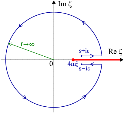
Figure 1: The integration contour in Eq. (6). The physical cut $\zeta\geq 4m_{\pi}^{2}$ of the Adler function $D(-\zeta)$ (4) is shown along the positive semiaxis of real $\zeta$.

In practice one deals with the Adler function $D(Q^{2})$ Adler , which is defined as the logarithmic derivative of the hadronic vacuum polarization function (1)

$$D(Q^{2})=-\frac{d\,\Pi(-Q^{2})}{d\ln Q^{2}},$$ (4)

with $Q^{2}=-q^{2}>0$ being the spacelike kinematic variable. Note that the subtraction point $q_{0}^{2}$ entering Eq. (2) does not appear in Eqs. (3) and (4). The widely employed dispersion relation for the Adler function follows immediately from Eqs. (2) and (4), specifically Adler

$$D(Q^{2})=Q^{2}\int\limits_{4m_{\pi}^{2}}^{\infty}\frac{R(\sigma)}{(\sigma+Q^{2})^{2}}\,d\sigma.$$ (5)

In particular, this dispersion relation enables one to extract the experimental prediction for the Adler function by making use of the corresponding experimental data on electron–positron annihilation into hadrons. However, to obtain the theoretical expression for the $R$–ratio itself, the relation inverse to Eq. (5) is required. The latter can be obtained by integrating Eq. (4) in finite limits, that yields Rad82 ; KP82

$$R(s)=\frac{1}{2\pi i}\lim_{\varepsilon\to 0_{+}}\int\limits_{s+i\varepsilon}^{s-i\varepsilon}D(-\zeta)\,\frac{d\zeta}{\zeta}.$$ (6)

Specifically, this equation relates the $R$–ratio to the theoretically calculable Adler function and provides a native way to properly account for the effects due to continuation of the spacelike perturbative results into the timelike domain. The integration contour in Eq. (6) lies in the region of analyticity of the integrand, see Fig. 1. Note also that the relation, which expresses the hadronic vacuum polarization function in terms of the Adler function can be obtained in a similar way, namely Pivovarov91

$$\Delta\Pi(-Q^{2}\!,\,-Q_{0}^{2})=-\int\limits_{Q_{0}^{2}}^{Q^{2}}D(\zeta)\frac{d\zeta}{\zeta},$$ (7)

where $Q^{2}$ and $Q_{0}^{2}$ stand for the spacelike kinematic variable and the subtraction point, respectively. Basically, Eqs. (2)–(7) constitute the complete set of relations, which express the functions on hand in terms of each other. It is worth mentioning here that, in general, the pattern of applications of the dispersion relations in theoretical particle physics is quite diverse. For example, among the latter are such issues as the refinement of chiral perturbation theory DRChPT ; Passemar , the accurate determination of parameters of resonances DRRes , the assessment of the hadronic light–by–light scattering Colangelo , as well as many others.

It is necessary to outline that the derivation of dispersion relations (2)–(7) is based only on the kinematics of the process on hand and involves neither model–dependent phenomenological assumptions nor additional approximations. In turn, the relations (2)–(7) impose a number of strict physical inherently nonperturbative constraints on the functions $\Pi(q^{2})$, $R(s)$, and $D(Q^{2})$, that should definitely be taken into account when one intends to go beyond the limits of applicability of the QCD perturbation theory. It is worthwhile to note that these nonperturbative restrictions have been merged with the corresponding perturbative input in the framework of dispersively improved perturbation theory (DPT) Book ; DPT1 ; DPT2 (its preliminary formulation was discussed in Ref. DPTPrelim ). In particular, the DPT enables one to overcome some intrinsic difficulties of the QCD perturbation theory and to extend its applicability range towards the infrared domain, see Ref. Book and references therein for the details.

In the framework of perturbation theory the Adler function (4) takes the form of the power series in the so–called QCD couplant $a^{(\ell)}_{\text{s}}(Q^{2})=\alpha^{(\ell)}_{\text{s}}(Q^{2})\,\beta_{0}/(4\pi)$, namely

$$D^{(\ell)}_{{\rm pert}}(Q^{2})=1+d^{(\ell)}_{{\rm pert}}(Q^{2}),\quad d^{(\ell)}_{{\rm pert}}(Q^{2})=\!\!\sum_{j=1}^{\ell}\!d_{j}\!\left[a^{(\ell)}_{\text{s}}(Q^{2})\!\right]^{j}\!.$$ (8)

In this equation $\ell$ specifies the loop level, $d_{1}=4/\beta_{0}$, $\beta_{0}=11-2n_{f}/3$, $n_{f}$ is the number of active flavors, and the common prefactor $N_{\text{c}}\sum_{f=1}^{n_{f}}Q_{f}^{2}$ is omitted throughout, where $N_{\text{c}}=3$ denotes the number of colors and $Q_{f}$ stands for the electric charge of $f$–th quark. The QCD couplant $a^{(\ell)}_{\text{s}}(Q^{2})$ entering Eq. (8) can be represented as the double sum

$$a^{(\ell)}_{\text{s}}(Q^{2})=\sum_{n=1}^{\ell}\sum_{m=0}^{n-1}b^{m}_{n}\,\frac{\ln^{m}(\ln z)}{\ln^{n}z},$$ (9)

where $z=Q^{2}/\Lambda^{2}$ and $b^{m}_{n}$ (the integer superscript $m$ is not to be confused with respective power) stands for the combination of the $\beta$ function perturbative expansion coefficients, specifically, $b^{0}_{1}=1$, $b^{0}_{2}=0$, $b^{1}_{2}=-\beta_{1}/\beta^{2}_{0}$, etc. The Adler function perturbative expansion coefficients $d_{j}$ were calculated up to the four–loop level ($1\leq j\leq 4$), see Ref. RPert4L and references therein, whereas for the five–loop coefficient $d_{5}$ only numerical estimation RPert5LEstim1 is available so far. The numerical values of the perturbative coefficients $d_{j}$ (8) are listed in Tab. 1. In turn, the $\beta$ function perturbative expansion coefficients $\beta_{j}$ have been calculated up to the five–loop level ($0\leq j\leq 4$), see Ref. Beta5L and references therein for the details.

Table 1: Numerical values of the Adler function perturbative expansion coefficients $d_{j}$ (8). In the last column the numerical estimation of the five–loop coefficient $d_{5}$ RPert5LEstim1 is listed.

$n_{f}$	$d_{1}$	$d_{2}$	$d_{3}$	$d_{4}$	$d_{5}$
0	0.3636	0.2626	0.8772	2.3743	5.40
1	0.3871	0.2803	0.7946	2.1884	4.70
2	0.4138	0.3005	0.7137	2.1466	3.74
3	0.4444	0.3239	0.5593	1.9149	2.52
4	0.4800	0.3513	0.2868	1.3440	1.16
5	0.5217	0.3836	$-0.1021$	0.6489	0.0256
6	0.5714	0.4225	$-0.7831$	$-0.8952$	0.267

In what follows the nonperturbative aspects of the strong interactions will be disregarded and a primary attention will be given to the theoretical description of the $R$–ratio of electron–positron annihilation into hadrons at moderate and high energies. For this purpose the effects due to the masses of the involved particles can be safely neglected (a discussion of the impact of such effects on the low–energy behavior of the functions $\Pi(q^{2})$, $R(s)$, and $D(Q^{2})$ can be found in, e.g., Refs. Book ; DPT1 ; DPT2 ; QCD8245 ; NPQCD71 ; C246 ). Additionally, for the scheme–dependent perturbative coefficients $\beta_{j}$ and $d_{j}$ the $\overline{\rm{MS}}$–scheme will be assumed and for the uncalculated yet five–loop coefficient $d_{5}$ its numerical estimation RPert5LEstim1 will be employed.

Thus, in the massless limit the relation (6) can be represented as (see also Ref. APT0a )

$$R^{(\ell)}(s)=1+r^{(\ell)}(s),\quad r^{(\ell)}(s)=\int\limits_{s}^{\infty}\!\rho^{(\ell)}(\sigma)\,\frac{d\sigma}{\sigma},$$ (10)

where

$$\rho^{(\ell)}(\sigma)=\frac{1}{2\pi i}\lim_{\varepsilon\to 0_{+}}\Bigl{[}d^{(\ell)}(-\sigma-i\varepsilon)-d^{(\ell)}(-\sigma+i\varepsilon)\!\Bigr{]}$$ (11)

stands for the spectral function and $d^{(\ell)}(Q^{2})$ denotes the $\ell$–loop strong correction to the Adler function. As mentioned above, only perturbative contributions will be retained in Eq. (11) hereinafter, that makes Eq. (10) identical to that of both the foregoing DPT Book ; DPT1 ; DPT2 and the so–called analytic perturbation theory (APT) APT0a ; APT0b . It has to be noted that, in general, the perturbative spectral function at small values of its argument may be altered by the terms of an intrinsically nonperturbative nature. For instance, the nonperturbative models discussed in Refs. PRD6264 ; Review ; MPLA1516 ; APTCSB constitute a superposition of the perturbative spectral function with the so–called “flat” terms (which by definition do not affect the corresponding perturbative results at high energies), whereas the models 12dAnQCD modify the low–energy behavior of the perturbative spectral function proceeding from certain phenomenological assumptions.

It is worthwhile to mention also that a “naive” approach to continue the spacelike perturbative result (8) into the timelike domain consists in merely identifying the timelike kinematic variable ($s=q^{2}$) with the spacelike one ($Q^{2}=-q^{2}$), i.e.,

$$R^{(\ell)}_{\text{naive}}(s)=D^{(\ell)}_{\text{pert}}(|s|)=1+\!\sum_{j=1}^{\ell}\!d_{j}\!\left[a^{(\ell)}_{\text{s}}(|s|)\!\right]^{j}\!.$$ (12)

However, as thoroughly discussed in Ref. Penn , this prescription yields a misleading result, which differs from the proper one (10) even in the deep ultraviolet asymptotic, see also Refs. Pi2Terms1 ; ProsperiAlpha ; RPert5LEstim1 as well as Book and references therein.

3 $R$–ratio at the one–loop level

Let us address now the $R$–ratio of electron–positron annihilation into hadrons at the one–loop level. As discussed in the previous Section, for this purpose the spectral function $\rho(\sigma)$ (11), which enters the pertinent integral representation (10), is required. Since the involved strong correction to the Adler function (8) takes a simple form at the one–loop level

$$d^{(1)}_{\text{pert}}(Q^{2})=d_{1}\,a^{(1)}_{\text{s}}(Q^{2}),\quad a^{(1)}_{\text{s}}(Q^{2})=\frac{1}{\ln(Q^{2}/\Lambda^{2})}$$ (13)

and

$$\lim_{\varepsilon\to 0_{+}}\ln(x\pm i\varepsilon)=\ln|x|\pm i\pi\theta(-x),$$ (14)

the calculation of $\rho^{(1)}(\sigma)$ (11) appears to be quite straightforward. Specifically, the one–loop spectral function (11) for the positive values of its argument reads

$$\rho^{(1)}(\sigma)=d_{1}\,\frac{1}{2\pi i}\left[\frac{1}{\ln(\sigma/\Lambda^{2})-i\pi}-\frac{1}{\ln(\sigma/\Lambda^{2})+i\pi}\right]\!\!,$$ (15)

that, in turn, can be represented as

$$\rho^{(1)}(\sigma)=d_{1}\bar{\rho}^{(1)}_{1}(\sigma),\quad\bar{\rho}^{(1)}_{1}(\sigma)=\frac{1}{y^{2}+\pi^{2}},\quad y=\ln\!\biggl{(}\!\frac{\sigma}{\Lambda^{2}}\!\biggr{)}\!.$$ (16)

In these equations $\theta(x)$ is the Heaviside unit step function [i.e., $\theta(x)=1$ if $x\geq 0$ and $\theta(x)=0$ otherwise], $d_{1}=4/\beta_{0}$, and $\beta_{0}=11-2n_{f}/3$. The plot of the one–loop spectral function $\bar{\rho}^{(1)}_{1}(\sigma)$ (16) is displayed in Fig. 2. As one can infer from this Figure, the function on hand assumes the values in the interval $0\leq\bar{\rho}^{(1)}_{1}(\sigma)\leq 1/\pi^{2}$ and decreases as $1/y^{2}$ in both ultraviolet ($y\to\infty$) and infrared ($y\to-\infty$) asymptotics.

Then, the corresponding one–loop strong correction to the $R$–ratio can also be easily obtained in an explicit form. Specifically, the integration (10) of the one–loop spectral function (16) yields

$$r^{(1)}(s)=d_{1}a^{(1)}_{\text{\scriptsize{TL}}}(s),\quad a^{(1)}_{\text{\scriptsize{TL}}}(s)=\frac{1}{2}-\frac{1}{\pi}\arctan\!\left(\frac{\ln w}{\pi}\right)\!,$$ (17)

where $w=s/\Lambda^{2}$. The function $a^{(1)}_{\text{\scriptsize{TL}}}(s)$ (17) constitutes the one–loop couplant, which properly accounts for the effects due to continuation of the spacelike perturbative expression (13) into the timelike domain. It is worthwhile to note here that Eq. (17) has first appeared in Ref. Schrempp80 and only afterwards was derived in Refs. Rad82 ; Pivovarov91 ; APT0a .

Figure 3 A displays the one–loop “timelike” effective couplant $a^{(1)}_{\text{\scriptsize{TL}}}(s)$ (17) and the “naive” continuation of the one–loop perturbative couplant $a^{(1)}_{\text{s}}(Q^{2})$ (13) into the timelike domain (12). As one can infer from this Figure, at high energies the two couplants approach each other. At the same time, at moderate energies the deviation between the functions on hand becomes significant, whereas in the infrared domain their behavior turns out to be qualitatively different. Specifically, the function $a^{(1)}_{\text{s}}(|s|)$ (13) diverges at low energies due to the infrared unphysical singularities, whereas $a^{(1)}_{\text{\scriptsize{TL}}}(s)$ (17) is a smooth monotone decreasing function of its argument, which contains no singularities for $s>0$.

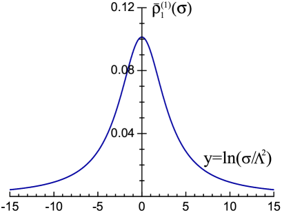
Figure 2: The one–loop spectral function $\bar{\rho}^{(1)}_{1}(\sigma)$ (16).

A somewhat simpler but approximate form of the strong correction to the $R$–ratio can be obtained by its further re–expansion. Specifically, for this purpose one splits the entire energy range $0<s<\infty$ into three intervals (namely, $\ln w<-\pi$, $-\pi<\ln w<\pi$, and $\ln w>\pi$) and applies the Taylor expansion to $r(s)$ in each of those intervals. At the one–loop level the implementation of these steps for the expression (17) yields

$$a^{(1)}_{\text{\scriptsize{TL}}}(s) \simeq 1+\frac{1}{\ln w}-\frac{1}{3}\frac{\pi^{2}}{\ln^{3}w}+\mathcal{O}\!\!\left(\!\frac{1}{\ln^{5}w}\!\right)\!\!,\quad\ln w<-\pi,$$ (18)

$$a^{(1)}_{\text{\scriptsize{TL}}}(s) \simeq\frac{1}{2}-\frac{\ln w}{\pi^{2}}+\frac{1}{3}\frac{\ln^{3}w}{\pi^{4}}+\mathcal{O}\!\Bigl{(}\!\ln^{5}w\!\Bigr{)}\!,\quad-\pi<\ln w<\pi,$$ (19)

$$a^{(1)}_{\text{\scriptsize{TL}}}(s) \simeq\frac{1}{\ln w}-\frac{1}{3}\frac{\pi^{2}}{\ln^{3}w}+\mathcal{O}\!\!\left(\!\frac{1}{\ln^{5}w}\!\right)\!\!,\quad\ln w>\pi,$$ (20)

where $w=s/\Lambda^{2}$. In particular, as one can infer from Fig. 3 B, the re–expansions (18)–(20) may provide an accurate approximation of the function (17) in the aforementioned energy intervals, if the number of retained terms is large enough. However, as one can note, the convergence of the re–expansions (18)–(20) becomes worse when the energy scale approaches the delimiting values $\sqrt{s}/\Lambda=\exp(\pm\pi/2)$, see also discussion of this issue in Sect. 6.

       

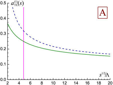
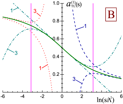
Figure 3: Plot A: The one–loop “timelike” effective couplant $a^{(1)}_{\text{\tiny{TL}}}(s)$ [Eq. (17), solid curve] and the naive continuation of the one–loop perturbative couplant into the timelike domain $a^{(1)}_{\text{s}}(|s|)$ [Eq. (13), dashed curve]. Plot B: The one–loop “timelike” effective couplant $a^{(1)}_{\text{\tiny{TL}}}(s)$ [Eq. (17), solid curve] and its re–expansions at various energy intervals: $\ln w<-\pi$ [Eq. (18), dotted curves], $-\pi<\ln w<\pi$ [Eq. (19), dot–dashed curves], and $\ln w>\pi$ [Eq. (20), dashed curves]. Numerical labels indicate the highest absolute value of the power of $\ln w$ retained in the re–expansions on hand. The boundaries of the convergence ranges of Eqs. (18)–(20) are marked by vertical solid lines.

In fact, there is another equivalent way to obtain the re–expansion of the strong correction to the $R$–ratio at high energies. Specifically, instead of following the lines described above, one can expand the corresponding spectral function $\rho^{(\ell)}(\sigma)$ (11) and then perform the integration in Eq. (10). In particular, at the one–loop level the Taylor expansion of $\bar{\rho}^{(1)}_{1}(\sigma)$ (16) for $\sqrt{\sigma}/\Lambda>\exp(\pi/2)$ reads

$$\bar{\rho}^{(1)}_{1}(\sigma)\simeq\frac{1}{y^{2}}-\frac{\pi^{2}}{y^{4}}+\mathcal{O}\!\biggl{(}\frac{1}{y^{6}}\biggr{)}\!,\qquad y=\ln\!\biggl{(}\!\frac{\sigma}{\Lambda^{2}}\!\biggr{)}\!,$$ (21)

that, after its integration in Eq. (10), yields the result identical to Eq. (20). It is the latter prescription that will be employed in the next Section for the derivation of an approximate expression for the $R$–ratio at high energies at an arbitrary loop level.

4 Re–expansion of the $R$–ratio at high energies: $\pi^{2}$–terms

As outlined in Sect. 2, the strong correction to the $R$–ratio of electron–positron annihilation into hadrons (10) can be represented as

$$r(s)=\int\limits_{s}^{\infty}\!\rho(\sigma)\,\frac{d\sigma}{\sigma}=\int\limits_{\ln w}^{\infty}\rho_{y}(y)\,dy,\qquad w=\frac{s}{\Lambda^{2}},$$ (22)

where $y=\ln(\sigma/\Lambda^{2})$ and $\rho_{y}(y)=\rho\bigl{[}\Lambda^{2}\exp(y)\bigr{]}$ denotes the corresponding spectral function (11)

$$\rho_{y}(y)=\frac{1}{2\pi i}\,\Bigl{[}d_{y}(y-i\pi)-d_{y}(y+i\pi)\Bigr{]}\!,$$ (23)

with Eq. (14) being employed. In Eq. (23) $d_{y}(y)=d\bigl{[}\Lambda^{2}\exp(y)\bigr{]}$ stands for the strong correction to the Adler function being expressed in terms of $y=\ln(\sigma/\Lambda^{2})$. Applying to the latter the Taylor expansion

$$d_{y}(y\pm i\pi)=d_{y}(y)+\sum_{n=1}^{\infty}\!\frac{(\pm i\pi)^{n}}{n!}\frac{d^{n}}{dy^{n}}\,d_{y}(y),\quad|y|>\pi,$$ (24)

one can approximate the spectral function (23) by

$$\rho_{y}(y)=-\frac{d}{dy}\,d_{y}(y)-\sum_{n=1}^{\infty}\frac{(-1)^{n}\pi^{2n}}{(2n+1)!}\,\frac{d^{2n+1}}{dy^{2n+1}}\,d_{y}(y).$$ (25)

Therefore, for $\sqrt{s}/\Lambda>\exp(\pi/2)\simeq 4.81$ the strong correction to the $R$–ratio (22) acquires the following form

$$r(s)=d(|s|)+\sum_{n=1}^{\infty}\frac{(-1)^{n}\pi^{2n}}{(2n+1)!}\,\frac{d^{2n}}{dy^{2n}}\,d_{y}(y)\Biggr{|}_{y=\ln w}\!.$$ (26)

In particular, this equation implies that the strong correction to the $R$–ratio, being re–expanded at high energies, reproduces the naive continuation of the Adler function into the timelike domain [the first term on the right–hand side of Eq. (26)] and additionally produces an infinite number of the so–called $\pi^{2}$–terms.

Then, at the $\ell$–loop level the perturbative expression for the strong correction to the Adler function reads (8)

$$d^{(\ell)}_{y}(y)=\sum_{j=1}^{\ell}d_{j}\left[a^{(\ell)}_{y}(y)\right]^{j}\!,$$ (27)

where $a^{(\ell)}_{y}(y)=a^{(\ell)}_{\text{s}}\bigl{[}\Lambda^{2}\exp(y)\bigr{]}$ is the $\ell$–loop perturbative couplant being expressed in terms of $y=\ln(\sigma/\Lambda^{2})$. Since the latter satisfies the renormalization group equation

$$\frac{d}{dy}\,a^{(\ell)}_{y}(y)=-\sum_{j=0}^{\ell-1}B_{j}\!\left[a^{(\ell)}_{y}(y)\right]^{j+2},\qquad B_{j}=\frac{\beta_{j}}{\beta^{j+1}_{0}},$$ (28)

the $n$–th derivative of the $j$–th power of the $\ell$–loop couplant takes the form

$$\frac{d^{n}}{dy^{n}}\!\left[a^{(\ell)}_{y}(y)\right]^{j} \!\!=(-1)^{n}\!\sum_{k_{1}=0}^{\ell-1}\!\ldots\!\sum_{k_{n}=0}^{\ell-1}\!\left[a^{(\ell)}_{y}(y)\!\right]^{j+n+k_{1}+\ldots+k_{n}}\!\times$$

$$\times\!\!\left(\prod_{p=1}^{n}B_{k_{p}}\!\!\right)\!\!\!\left[\prod_{t=0}^{n-1}\Bigl{(}\!j+t+k_{1}+\ldots+k_{t}\!\Bigr{)}\!\!\right]\!\!.$$ (29)

Thus, at high energies the $\ell$–loop strong correction to the $R$–ratio (22) can be approximated by (see also Ref. Pi2termsHO )

$$r^{(\ell)}(s) =\sum_{j=1}^{\ell}d_{j}\left[a^{(\ell)}_{{\rm s}}(|s|)\right]^{j}-\sum_{j=1}^{\ell}d_{j}\sum_{n=1}^{\infty}\!\frac{(-1)^{n+1}\pi^{2n}}{(2n+1)!}\times$$

$$\times\!\!\sum_{k_{1}=0}^{\ell-1}\!\ldots\!\sum_{k_{2n}=0}^{\ell-1}\!\!\left(\prod_{p=1}^{2n}B_{k_{p}}\!\!\right)\!\!\!\left[\prod_{t=0}^{2n-1}\!\!\Bigl{(}j+t+k_{1}+k_{2}+\ldots+k_{t}\Bigr{)}\!\!\right]\!\!\!\times$$

$$\times\!\!\Bigl{[}a^{(\ell)}_{{\rm s}}(|s|)\Bigr{]}^{j+2n+k_{1}+k_{2}+\ldots+k_{2n}},\qquad\frac{\sqrt{s}}{\Lambda}>\exp\!\biggl{(}\!\frac{\pi}{2}\!\biggr{)}\!.$$ (30)

The obtained re–expansion of the strong correction to the $R$–ratio (4) constitutes the sum of naive continuation of the strong correction to the Adler function into the timelike domain (12) and an infinite number of the $\pi^{2}$–terms. Equation (4) explicitly proves the fact that at any given loop level the re–expansion of the strong correction to the $R$–ratio at high energies can be reduced to the form of power series in the naive continuation of the perturbative couplant into the timelike domain $a^{(\ell)}_{\text{s}}(|s|)$. As one can also note, in the re–expansion (4) the coefficients $d_{j}$ corresponding to various orders of perturbation theory turn out to be all mixed up, i.e., the $\ell$–loop contribution to Eq. (10) appears to be re–distributed over the higher–order terms.

Table 2: Numerical values of the coefficients $\delta_{j}$ (32) embodying the contributions of the relevant $\pi^{2}$–terms (4). The last column employs the numerical estimation of the Adler function perturbative expansion coefficient $d_{5}$ RPert5LEstim1 .

$n_{f}$	$\delta_{1}$	$\delta_{2}$	$\delta_{3}$	$\delta_{4}$	$\delta_{5}$	$\delta_{6}$	$\delta_{7}$
0	0.0000	0.0000	1.1963	5.1127	20.455	69.081	45.7
1	0.0000	0.0000	1.2735	5.4298	18.880	56.819	7.02
2	0.0000	0.0000	1.3613	5.7583	17.118	48.532	$-$35.7
3	0.0000	0.0000	1.4622	6.0851	13.519	30.365	$-$82.5
4	0.0000	0.0000	1.5791	6.3850	6.910	$-$3.843	$-$115.7
5	0.0000	0.0000	1.7165	6.6090	$-$3.187	$-$45.692	$-$83.0
6	0.0000	0.0000	1.8799	6.6638	$-$21.168	$-$120.010	142.5

As discussed earlier, if the number of terms retained in Eq. (4) is large enough, then it can provide a rather accurate approximation of the strong correction to the $R$–ratio (10) for $\sqrt{s}/\Lambda>\exp(\pi/2)\simeq 4.81$. However, one usually truncates the re–expansion (4) at the order $\ell$, thereby neglecting all the higher–order $\pi^{2}$–terms, that results in the following expression commonly employed in practical applications:

$$R^{(\ell)}_{{\rm appr}}(s)=1+r^{(\ell)}_{{\rm appr}}(s),\quad r^{(\ell)}_{{\rm appr}}(s)=\!\sum_{j=1}^{\ell}r_{j}\!\left[a^{(\ell)}_{{\rm s}}(|s|)\right]^{j}\!,$$ (31)

where

$$r_{j}=d_{j}-\delta_{j}.$$ (32)

In this equation $d_{j}$ stand for the Adler function perturbative expansion coefficients (8), whereas $\delta_{j}$ embody the contributions of the relevant $\pi^{2}$–terms.

Equation (4) implies that the $\pi^{2}$–terms do not appear in the first and second orders of perturbation theory, namely,

$$\delta_{1}=0,\qquad\delta_{2}=0,$$ (33)

that makes $R^{(\ell)}_{{\rm appr}}(s)$ (31) identical to the naive expression $R^{(\ell)}_{{\rm naive}}(s)$ (12) for $\ell=1$ and $\ell=2$. Starting from the third order of perturbation theory (i.e., for $\ell\geq 3$) the coefficients $\delta_{j}$ (32) are no longer vanishing and constitute a combination of the pertinent perturbative expansion coefficients $d_{j}$ and $\beta_{j}$ of the first $(\ell-2)$ orders. Specifically, the third–order and fourth–order coefficients read Pi2Terms1 ; RPert5LEstim1 ; ProsperiAlpha

$$\delta_{3}=\frac{\pi^{2}}{3}d_{1}B_{0}^{2}=\frac{\pi^{2}}{3}d_{1}$$ (34)

and

$$\delta_{4}=\frac{\pi^{2}}{3}\!\left(\frac{5}{2}d_{1}B_{0}B_{1}+3d_{2}B_{0}^{2}\!\right)\!=\frac{\pi^{2}}{3}\!\left(\frac{5}{2}d_{1}B_{1}+3d_{2}\!\right)\!\!,$$ (35)

respectively. In these equations $d_{j}$ denote the Adler function perturbative expansion coefficients (8), whereas $B_{j}=\beta_{j}/\beta^{j+1}_{0}$ stands for the combination of perturbative coefficients of the renormalization group $\beta$ function. In turn, at the fifth and sixth orders the coefficients $\delta_{j}$ (32) can be represented as RPert5LEstim1 ; Book ; Pi2termsHO

$$\delta_{5} =\frac{\pi^{2}}{3}\biggl{[}\frac{3}{2}d_{1}\!\Bigl{(}B_{1}^{2}+2B_{2}\!\Bigr{)}+7d_{2}B_{1}+6d_{3}\biggr{]}\!-\frac{\pi^{4}}{5}d_{1},$$ (36)

$$\delta_{6} =\frac{\pi^{2}}{3}\biggl{[}\frac{7}{2}d_{1}\!\Bigl{(}B_{1}B_{2}+B_{3}\!\Bigr{)}+4d_{2}\left(B_{1}^{2}+2B_{2}\right)+$$

$$+\frac{27}{2}d_{3}B_{1}+10d_{4}\biggr{]}\!-\frac{\pi^{4}}{5}\!\left(\frac{77}{12}d_{1}B_{1}+5d_{2}\!\right)\!\!.$$ (37)

The seventh– and eighth–order coefficients $\delta_{j}$ (32) have recently been calculated as well, specifically Book ; Pi2termsHO

$$\delta_{7} =\frac{\pi^{2}}{3}\Biggl{[}4d_{1}\!\left(\!B_{1}B_{3}+\frac{1}{2}B_{2}^{2}+B_{4}\!\right)+9d_{2}\Bigl{(}\!B_{1}B_{2}+B_{3}\!\Bigr{)}+$$

$$+\frac{15}{2}d_{3}\Bigl{(}\!B_{1}^{2}+2B_{2}\!\Bigr{)}+22d_{4}B_{1}+15d_{5}\Biggr{]}-$$

$$-\frac{\pi^{4}}{5}\left[\frac{5}{6}d_{1}\Bigl{(}\!17B_{1}^{2}+12B_{2}\!\Bigr{)}+\frac{57}{2}d_{2}B_{1}+15d_{3}\right]\!+\frac{\pi^{6}}{7}d_{1}$$ (38)

and

$$\delta_{8} =\frac{\pi^{2}}{3}\Biggl{[}\frac{9}{2}d_{1}\Bigl{(}\!B_{1}B_{4}+B_{2}B_{3}+B_{5}\!\Bigr{)}+$$

$$+10d_{2}\!\left(\!B_{1}B_{3}+\frac{1}{2}B_{2}^{2}+B_{4}\!\right)+\frac{33}{2}d_{3}\Bigl{(}\!B_{1}B_{2}+B_{3}\!\Bigr{)}+$$

$$+12d_{4}\Bigl{(}\!B_{1}^{2}+2B_{2}\!\Bigr{)}+\frac{65}{2}d_{5}B_{1}+21d_{6}\Biggr{]}-$$

$$-\frac{\pi^{4}}{5}\Biggl{[}\frac{15}{8}d_{1}\!\Bigl{(}\!7B_{1}^{3}+22B_{1}B_{2}+8B_{3}\!\Bigr{)}+$$

$$+\frac{5}{12}d_{2}\Bigl{(}\!139B_{1}^{2}+96B_{2}\!\Bigr{)}+\frac{319}{4}d_{3}B_{1}+35d_{4}\Biggr{]}+$$

$$+\frac{\pi^{6}}{7}\left(\frac{223}{20}d_{1}B_{1}+7d_{2}\right)\!.$$ (39)

The explicit expressions for the coefficients $\delta_{j}$ (32) at the higher orders can be found in App. C of Ref. Book .

Table 3: Numerical values of the coefficients $r_{j}$ of the re–expanded approximate $R$–ratio (31). The last column employs the numerical estimation of the Adler function perturbative expansion coefficient $d_{5}$ RPert5LEstim1 .

$n_{f}$	$r_{1}=d_{1}$	$r_{2}=d_{2}$	$r_{3}=d_{3}-\delta_{3}$	$r_{4}=d_{4}-\delta_{4}$	$r_{5}=d_{5}-\delta_{5}$
0	0.3636	0.2626	$-$0.3191	$-$2.7383	$-$15.1
1	0.3871	0.2803	$-$0.4788	$-$3.2413	$-$14.2
2	0.4138	0.3005	$-$0.6476	$-$3.6116	$-$13.4
3	0.4444	0.3239	$-$0.9028	$-$4.1703	$-$11.0
4	0.4800	0.3513	$-$1.2923	$-$5.0409	$-$5.75
5	0.5217	0.3836	$-$1.8186	$-$5.9601	3.21
6	0.5714	0.4225	$-$2.6630	$-$7.5590	21.4

Table 4: The relative weight $(1+|d_{j}/\delta_{j}|)^{-1}\!\times\!100\%$ of the $\pi^{2}$–terms in the coefficients $r_{j}$ of the re–expanded approximate $R$–ratio (31). The last column employs the numerical estimation of the Adler function perturbative expansion coefficient $d_{5}$ RPert5LEstim1 .

$n_{f}$	$j=1$	$j=2$	$j=3$	$j=4$	$j=5$
0	$0.00\,\%$	$0.00\,\%$	$57.7\,\%$	$68.3\,\%$	79.1$\,\%$
1	$0.00\,\%$	$0.00\,\%$	$61.6\,\%$	$71.3\,\%$	80.1$\,\%$
2	$0.00\,\%$	$0.00\,\%$	$65.6\,\%$	$72.8\,\%$	82.1$\,\%$
3	$0.00\,\%$	$0.00\,\%$	$72.3\,\%$	$76.1\,\%$	84.3$\,\%$
4	$0.00\,\%$	$0.00\,\%$	$84.6\,\%$	$82.6\,\%$	85.6$\,\%$
5	$0.00\,\%$	$0.00\,\%$	$94.4\,\%$	$91.1\,\%$	99.2$\,\%$
6	$0.00\,\%$	$0.00\,\%$	$70.6\,\%$	$88.2\,\%$	98.8$\,\%$

Table 2 presents the numerical values of the first seven coefficients $\delta_{j}$ (32), which embody the contributions of the relevant $\pi^{2}$–terms (4). Tables 1 and 2 make it evident that in Eq. (31) the coefficients $\delta_{j}$ can in no way be regarded as small corrections to the Adler function perturbative expansion coefficients $d_{j}$ (8) for $j\geq 3$. On the contrary, the values of coefficients $\delta_{j}$ significantly exceed the values of respective perturbative coefficients $d_{j}$, thereby constituting the dominant contribution to the coefficients $r_{j}$ (32), see also Tabs. 3 and 4. As will be discussed below, eventually this results in an essential distortion of the re–expanded approximation $R^{(\ell)}_{\text{appr}}(s)$ (31) with respect to the naive expression $R^{(\ell)}_{\text{naive}}(s)$ (12). In particular, the higher–order terms of $R^{(\ell)}_{\text{appr}}(s)$ (31) turn out to be substantially amplified and even sign–reversed with respect to those of $R^{(\ell)}_{\text{naive}}(s)$ (12), see Tabs. 1 and 3. It is worthwhile to note also that, as one can infer from Tabs. 2 and 4, the values of coefficients $\delta_{j}$ rapidly increase as the order $j$ increases, that makes the loop convergence of $R^{(\ell)}_{\text{appr}}(s)$ (31) worse than that of both $R^{(\ell)}(s)$ (10) and $R^{(\ell)}_{\text{naive}}(s)$ (12), see Sect. 6 for the details.

5 Spectral function at the higher–loop levels

It is certainly desirable to leave the truncated re–expanded approximation $R^{(\ell)}_{\text{appr}}(s)$ (31) aside and have the function $R^{(\ell)}(s)$ (10) calculated in a straightforward way beyond the one–loop level. To achieve this objective, the corresponding explicit expression for the involved spectral function $\rho^{(\ell)}(\sigma)$ (11) is required. Despite the latter becomes rather cumbrous for $\ell\geq 2$, the following method enables one to calculate $\rho^{(\ell)}(\sigma)$ explicitly at an arbitrary loop level.

Specifically, it proves to be convenient to express the spectral function $\rho^{(\ell)}(\sigma)$ (11) in terms of the so–called “partial” spectral functions $\bar{\rho}^{(\ell)}_{j}(\sigma)$ corresponding to the $j$–th power of the $\ell$–loop perturbative couplant (9), namely

$$\rho^{(\ell)}(\sigma)=\sum_{j=1}^{\ell}d_{j}\,\bar{\rho}^{(\ell)}_{j}(\sigma),$$ (40)

where

$$\bar{\rho}^{(\ell)}_{j}(\sigma)=\frac{1}{2\pi i}\lim_{\varepsilon\to 0_{+}}\!\left\{\!\!\left[a^{(\ell)}_{\text{s}}\!(-\sigma-i\varepsilon)\right]^{j}\!\!-\!\left[a^{(\ell)}_{\text{s}}\!(-\sigma+i\varepsilon)\right]^{j}\!\right\}\!\!.$$ (41)

To obtain the partial spectral function $\bar{\rho}^{(\ell)}_{j}(\sigma)$ (41) for any $j\geq 1$ it appears to be enough to calculate only the real and imaginary parts of the $\ell$–loop couplant $a^{(\ell)}_{\text{s}}(Q^{2})$ at the edges of its cut:

$$\lim_{\varepsilon\to 0_{+}}a^{(\ell)}_{\text{s}}(-\sigma\pm i\varepsilon)=a^{(\ell)}_{\text{\scriptsize{Re}}}(\sigma)\mp i\pi a^{(\ell)}_{\text{\scriptsize{Im}}}(\sigma).$$ (42)

Here $a^{(\ell)}_{\text{\scriptsize{Re}}}(\sigma)$ and $a^{(\ell)}_{\text{\scriptsize{Im}}}(\sigma)$ are the real functions of their arguments and $\sigma\geq 0$ is assumed. For positive integer values of $j$ the following equation holds

$$\lim_{\varepsilon\to 0_{+}}\Bigl{[}a^{(\ell)}_{\text{s}}(-\sigma\pm i\varepsilon)\Bigr{]}^{j} =\sum_{k=0}^{j}\binom{j}{k}\,(\mp i\pi)^{k}\times$$

$$\times\Bigl{[}a^{(\ell)}_{\text{\scriptsize{Re}}}(\sigma)\Bigr{]}^{j-k}\,\Bigl{[}a^{(\ell)}_{\text{\scriptsize{Im}}}(\sigma)\Bigr{]}^{k},$$ (43)

with

$$\binom{n}{m}=\frac{n!}{m!\,(n-m)!}$$ (44)

being the binomial coefficient. Then, it is convenient to isolate in Eq. (5) its real and imaginary parts, specifically

$$\lim_{\varepsilon\to 0_{+}}\Bigl{[}a^{(\ell)}_{\text{s}}(-\sigma\pm i\varepsilon)\Bigr{]}^{j} =\sum_{k=0}^{K(j+1)}\binom{j}{2k}\,(-1)^{k}(\pi)^{2k}\times$$

$$\times\Bigl{[}a^{(\ell)}_{\text{\scriptsize{Re}}}(\sigma)\Bigr{]}^{j-2k}\,\Bigl{[}a^{(\ell)}_{\text{\scriptsize{Im}}}(\sigma)\Bigr{]}^{2k}\mp\quad$$

$$\mp i\pi\sum_{k=0}^{K(j)}\binom{j}{2k+1}\,(-1)^{k}(\pi)^{2k}\times$$

$$\times\Bigl{[}a^{(\ell)}_{\text{\scriptsize{Re}}}(\sigma)\Bigr{]}^{j-2k-1}\,\Bigl{[}a^{(\ell)}_{\text{\scriptsize{Im}}}(\sigma)\Bigr{]}^{2k+1},$$ (45)

where

$$K(j)=\frac{j-2}{2}+\frac{j\;\mbox{mod}\;2}{2}$$ (46)

and $(j\;\mbox{mod}\;n)$ denotes the remainder on division of $j$ by $n$. Therefore, the partial spectral function (41) reads (see also Refs. Review ; QCDDPT1 )

$$\bar{\rho}^{(\ell)}_{j}(\sigma) =\sum_{k=0}^{K(j)}\binom{j}{2k+1}\,(-1)^{k}\,\pi^{2k}\times$$

$$\times\Bigl{[}a^{(\ell)}_{\text{\scriptsize{Re}}}(\sigma)\Bigr{]}^{j-2k-1}\,\Bigl{[}a^{(\ell)}_{\text{\scriptsize{Im}}}(\sigma)\Bigr{]}^{2k+1},$$ (47)

with $\sigma\geq 0$ and $j\geq 1$ being assumed. In particular, the first five relations (5) acquire a compact form

$$\bar{\rho}^{(\ell)}_{1}(\sigma) =a^{(\ell)}_{\text{\scriptsize{Im}}}(\sigma),$$ (48)

$$\bar{\rho}^{(\ell)}_{2}(\sigma) =2\,a^{(\ell)}_{\text{\scriptsize{Im}}}(\sigma)\,a^{(\ell)}_{\text{\scriptsize{Re}}}(\sigma),$$ (49)

$$\bar{\rho}^{(\ell)}_{3}(\sigma) =a^{(\ell)}_{\text{\scriptsize{Im}}}(\sigma)\left\{\!3\Bigl{[}a^{(\ell)}_{\text{\scriptsize{Re}}}(\sigma)\Bigr{]}^{2}\!-\pi^{2}\Bigl{[}a^{(\ell)}_{\text{\scriptsize{Im}}}(\sigma)\Bigr{]}^{2}\right\},$$ (50)

$$\bar{\rho}^{(\ell)}_{4}(\sigma) =4\,a^{(\ell)}_{\text{\scriptsize{Im}}}(\sigma)\,a^{(\ell)}_{\text{\scriptsize{Re}}}(\sigma)\left\{\!\Bigl{[}a^{(\ell)}_{\text{\scriptsize{Re}}}(\sigma)\Bigr{]}^{2}\!-\pi^{2}\Bigl{[}a^{(\ell)}_{\text{\scriptsize{Im}}}(\sigma)\Bigr{]}^{2}\right\},$$ (51)

$$\bar{\rho}^{(\ell)}_{5}(\sigma) =a^{(\ell)}_{\text{\scriptsize{Im}}}(\sigma)\biggl{\{}\!5\Bigl{[}a^{(\ell)}_{\text{\scriptsize{Re}}}(\sigma)\Bigr{]}^{4}\!-10\pi^{2}\Bigl{[}a^{(\ell)}_{\text{\scriptsize{Im}}}(\sigma)a^{(\ell)}_{\text{\scriptsize{Re}}}(\sigma)\Bigr{]}^{2}$$

$$+\pi^{4}\Bigl{[}a^{(\ell)}_{\text{\scriptsize{Im}}}(\sigma)\Bigr{]}^{4}\biggr{\}}.$$ (52)

In turn, the $\ell$–loop functions $a^{(\ell)}_{\text{\scriptsize{Re}}}(\sigma)$ and $a^{(\ell)}_{\text{\scriptsize{Im}}}(\sigma)$ entering Eq. (5) can also be explicitly calculated in a similar way. Specifically, as mentioned in Sect. 2, the perturbative QCD couplant $a^{(\ell)}_{\text{s}}(Q^{2})$ can be represented as the double sum (9) comprised of the functions

$$\bar{a}_{n}^{m}(Q^{2})=\frac{\ln^{m}(\ln z)}{\ln^{n}z},\qquad z=\frac{Q^{2}}{\Lambda^{2}}.$$ (53)

It is worthwhile to decompose the function $\bar{a}_{n}^{m}(Q^{2})$ (53) at the edges of its cut into the real and imaginary parts, namely

$$\lim_{\varepsilon\to 0_{+}}\bar{a}_{n}^{m}(-\sigma\pm i\varepsilon)=u_{n}^{m}(\sigma)\mp i\pi v_{n}^{m}(\sigma),$$ (54)

where $u_{n}^{m}(\sigma)$ and $v_{n}^{m}(\sigma)$ are the real functions of their arguments and $\sigma\geq 0$ is assumed. Therefore, the functions $a^{(\ell)}_{\text{\scriptsize{Re}}}(\sigma)$ and $a^{(\ell)}_{\text{\scriptsize{Im}}}(\sigma)$ (42) take the following form

$$a^{(\ell)}_{\text{\scriptsize{Re}}}(\sigma) =\sum_{n=1}^{\ell}\sum_{m=0}^{n-1}b^{m}_{n}\,u_{n}^{m}(\sigma),$$ (55)

$$a^{(\ell)}_{\text{\scriptsize{Im}}}(\sigma) =\sum_{n=1}^{\ell}\sum_{m=0}^{n-1}b^{m}_{n}\,v_{n}^{m}(\sigma).$$ (56)

On the left–hand side of Eq. (53) and in Eqs. (54)–(56) the integer superscripts $m$ are not to be confused with respective powers, whereas the coefficients $b^{m}_{n}$ have been specified in Eq. (9).

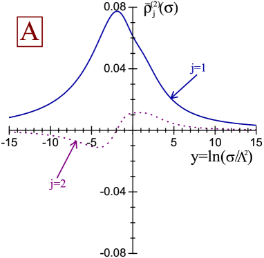
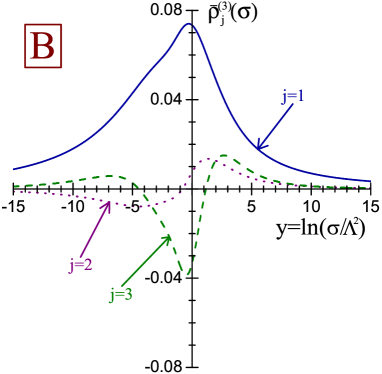
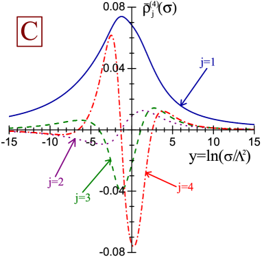
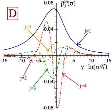
Figure 4: The partial spectral functions $\bar{\rho}^{(\ell)}_{j}(\sigma)$ (5) corresponding to the $j$–th power ($1\leq j\leq\ell$) of the $\ell$–loop ($2\leq\ell\leq 5$) perturbative QCD couplant $a^{(\ell)}_{{\rm s}}(Q^{2})$. Plot A: two–loop level ($\ell=2$, $1\leq j\leq 2$). Plot B: three–loop level ($\ell=3$, $1\leq j\leq 3$), the function $\bar{\rho}^{(3)}_{3}(\sigma)$ is scaled by the factor of $10$. Plot C: four–loop level ($\ell=4$, $1\leq j\leq 4$), the functions $\bar{\rho}^{(4)}_{3}(\sigma)$ and $\bar{\rho}^{(4)}_{4}(\sigma)$ are scaled by the factors of $10$ and $10^{2}$, respectively. Plot D: five–loop level ($\ell=5$, $1\leq j\leq 5$), the functions $\bar{\rho}^{(5)}_{3}(\sigma)$, $\bar{\rho}^{(5)}_{4}(\sigma)$, and $\bar{\rho}^{(5)}_{5}(\sigma)$ are scaled by the factors of $10$, $10^{2}$, and $10^{2}$, respectively.

Then, to calculate the functions $u_{n}^{m}(\sigma)$ and $v_{n}^{m}(\sigma)$ entering Eqs. (55) and (56), it is convenient to split the left–hand side of Eq. (54) into two factors:

$$\lim_{\varepsilon\to 0_{+}}\bar{a}_{n}^{m}(-\sigma\pm i\varepsilon)=\lim_{\varepsilon\to 0_{+}}\Bigl{[}\bar{a}_{n}^{0}(-\sigma\pm i\varepsilon)\,\bar{a}_{0}^{m}(-\sigma\pm i\varepsilon)\!\Bigr{]}\!.$$ (57)

The first factor on the right–hand side of Eq. (57) reads

$$\lim_{\varepsilon\to 0_{+}}\bar{a}_{n}^{0}(-\sigma\pm i\varepsilon)=\frac{(y\mp i\pi)^{n}}{(y^{2}+\pi^{2})^{n}},\qquad y=\ln\biggl{(}\!\frac{\sigma}{\Lambda^{2}}\!\biggr{)}\!.$$ (58)

Proceeding along the same lines as earlier, one can cast the numerator on the right–hand side of this equation to

$$(y\mp i\pi)^{n} =\!\!\!\sum_{k=0}^{K(n+1)}\!\binom{n}{2k}(-1)^{k}\pi^{2k}y^{n-2k}\mp$$

$$\mp i\pi\!\!\sum_{k=0}^{K(n)}\!\binom{n}{2k+1}(-1)^{k}\pi^{2k}y^{n-2k-1},$$ (59)

with $K(n)$ being specified in Eq. (46). Hence, the functions $u_{n}^{m}(\sigma)$ and $v_{n}^{m}(\sigma)$ (54) for $m=0$ read

$$u_{n}^{0}(\sigma) =\frac{1}{(y^{2}+\pi^{2})^{n}}\sum_{k=0}^{K(n+1)}\!\binom{n}{2k}(-1)^{k}\pi^{2k}y^{n-2k},$$ (60)

$$v_{n}^{0}(\sigma) =\frac{1}{(y^{2}+\pi^{2})^{n}}\sum_{k=0}^{K(n)}\!\binom{n}{2k+1}(-1)^{k}\pi^{2k}y^{n-2k-1},$$ (61)

with $n\geq 1$ being assumed.

In turn, for $m\geq 1$ the second factor on the right–hand side of Eq. (57) takes the following form

$$\lim_{\varepsilon\to 0_{+}}\bar{a}_{0}^{m}(-\sigma\pm i\varepsilon)=\Bigl{[}\ln(y\pm i\pi)\Bigr{]}^{m},$$ (62)

where $y=\ln(\sigma/\Lambda^{2})$. Since for real $a$ and $b$

$$\ln(a\pm ib)=\ln\!\sqrt{\!a^{2}+b^{2}}\pm i\pi\!\!\left[\frac{1}{2}-\frac{1}{\pi}\arctan\!\left(\frac{a}{b}\right)\!\right]\!\!,\quad b>0,$$ (63)

Eq. (62) can be rewritten as

$$\lim_{\varepsilon\to 0_{+}}\bar{a}_{0}^{m}(-\sigma\pm i\varepsilon)=\sum\limits_{k=0}^{m}\binom{m}{k}(\pm i\pi)^{k}\Bigl{[}L_{1}(y)\Bigr{]}^{m-k}\,\Bigl{[}L_{2}(y)\Bigr{]}^{k},$$ (64)

where

$$L_{1}(y)=\ln\!\sqrt{y^{2}+\pi^{2}},\qquad L_{2}(y)=\frac{1}{2}-\frac{1}{\pi}\arctan\!\left(\frac{y}{\pi}\right)\!.$$ (65)

Following the same steps as above, one can cast Eq. (64) to

$$\lim_{\varepsilon\to 0_{+}}\bar{a}_{0}^{m}(-\sigma\pm i\varepsilon)=u_{0}^{m}(\sigma)\mp i\pi v_{0}^{m}(\sigma),$$ (66)

where

$$u_{0}^{m}(\sigma) =\!\sum\limits_{k=0}^{K(m+1)}\binom{m}{2k}(-1)^{k}\pi^{2k}\times$$

$$\times\Bigl{[}L_{1}(y)\Bigr{]}^{m-2k}\,\Bigl{[}L_{2}(y)\Bigr{]}^{2k},$$ (67)

$$v_{0}^{m}(\sigma) =\!\sum\limits_{k=0}^{K(m)}\binom{m}{2k+1}(-1)^{k+1}\pi^{2k}\times$$

$$\times\Bigl{[}L_{1}(y)\Bigr{]}^{m-2k-1}\,\Bigl{[}L_{2}(y)\Bigr{]}^{2k+1},$$ (68)

$K(m)$ is defined in Eq. (46), and $m\geq 1$ is assumed.

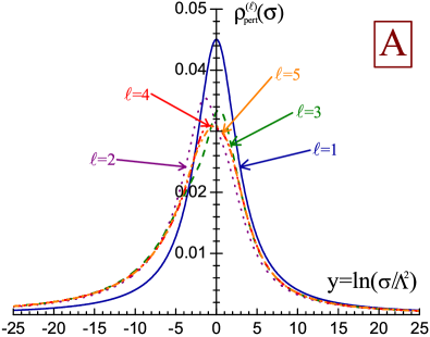
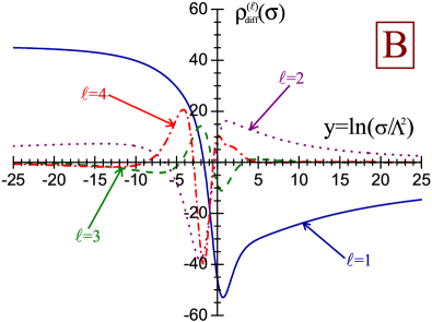
Figure 5: Plot A: The spectral function $\rho^{(\ell)}(\sigma)$ (5) at the first five loop levels ($1\leq\ell\leq 5$). Plot B: The relative difference $\rho^{(\ell)}_{\text{diff}}(\sigma)$ (74) between the $\ell$–loop and $(\ell+1)$–loop spectral functions (5) at various loop levels. The function $\rho^{(4)}_{\text{diff}}(\sigma)$ is scaled by the factor of $10$.

Therefore, the functions $u_{n}^{m}(\sigma)$ and $v_{n}^{m}(\sigma)$ (54) read

$$u_{n}^{m}(\sigma)=\begin{cases}u_{n}^{0}(\sigma),&\text{if $\,m=0$},\\[3.55658pt] u_{n}^{0}(\sigma)u_{0}^{m}(\sigma)-\pi^{2}v_{n}^{0}(\sigma)v_{0}^{m}(\sigma),\quad&\text{if $\,m\geq 1$},\end{cases}$$ (69)

and

$$v_{n}^{m}(\sigma)=\begin{cases}v_{n}^{0}(\sigma),&\text{if $\,m=0$},\\[3.55658pt] v_{n}^{0}(\sigma)u_{0}^{m}(\sigma)+u_{n}^{0}(\sigma)v_{0}^{m}(\sigma),\quad&\text{if $\,m\geq 1$},\end{cases}$$ (70)

with $n\geq 1$ being assumed. Thus, the explicit expression for the $\ell$–loop spectral function $\rho^{(\ell)}(\sigma)$ (40) takes the following form:

$$\rho^{(\ell)}(\sigma) =\sum_{j=1}^{\ell}d_{j}\sum_{k=0}^{K(j)}\binom{j}{2k+1}(-1)^{k}\,\pi^{2k}\times$$

$$\times\!\Biggl{[}\sum_{n=1}^{\ell}\sum_{m=0}^{n-1}b^{m}_{n}\,u_{n}^{m}(\sigma)\Biggr{]}^{j-2k-1}\times$$

$$\times\!\Biggl{[}\sum_{n=1}^{\ell}\sum_{m=0}^{n-1}b^{m}_{n}\,v_{n}^{m}(\sigma)\Biggr{]}^{2k+1},$$ (71)

where the functions $u_{n}^{m}(\sigma)$ and $v_{n}^{m}(\sigma)$ are specified in Eqs. (69) and (70), respectively.

The higher–loop partial spectral functions $\bar{\rho}^{(\ell)}_{j}(\sigma)$ (5), which correspond to the $j$–th power ($1\leq j\leq\ell$) of the $\ell$–loop ($2\leq\ell\leq 5$) perturbative QCD couplant $a^{(\ell)}_{\text{s}}(Q^{2})$, are displayed in Fig. 4. As one can infer from this Figure, the functions $\bar{\rho}^{(\ell)}_{j}(\sigma)$ (5) vanish at both $\sigma\to\infty$ and $\sigma\to 0$, the higher–order functions $\bar{\rho}^{(\ell)}_{j}(\sigma)$ ($j\geq 2$) being substantially suppressed with respect to those of the preceding orders. For example, Fig. 4 D implies that at the five–loop level the maximum value of the fifth–order function $\bar{\rho}^{(5)}_{5}(\sigma)$ is about three orders of magnitude less than the maximum value of the first–order function $\bar{\rho}^{(5)}_{1}(\sigma)$. In turn, as it will be discussed in the next Section, the fact that the function $\bar{\rho}^{(\ell)}_{j+1}(\sigma)$ is subdominant to $\bar{\rho}^{(\ell)}_{j}(\sigma)$ eventually results in an enhanced higher–loop stability of the proper expression for the $R$–ratio (10) at moderate and low energies with respect to both its naive form (12) and the commonly employed truncated re–expanded approximation (31).

The plots of the spectral function $\rho^{(\ell)}(\sigma)$ (5) at the first five loop levels ($1\leq\ell\leq 5$) are displayed in Fig. 5 A. As one can infer from this Figure, the function $\rho^{(\ell)}(\sigma)$ vanishes at both $\sigma\to\infty$ and $\sigma\to 0$. Specifically, at the higher–loop levels ($\ell\geq 2$)

$$\rho^{(\ell)}(\sigma)\simeq\frac{d_{1}}{y^{2}}+\mathcal{O}\left(\frac{1}{y^{3}}\right)\!,\quad y=\ln\biggl{(}\frac{\sigma}{\Lambda^{2}}\biggr{)}\!,\quad y\to\infty$$ (72)

and

$$\rho^{(\ell)}(\sigma)\simeq\frac{d_{1}(1+B_{1})}{y^{2}}+\mathcal{O}\left(\frac{1}{y^{3}}\right)\!,\qquad y\to-\infty.$$ (73)

Additionally, Fig. 5 A implies that the range of $y$, where the difference between $\rho^{(\ell)}(\sigma)$ and $\rho^{(\ell+1)}(\sigma)$ is sizable, is located in the vicinity of $y=0$ and becomes smaller at larger $\ell$. This issue is also elucidated by Fig. 5 B, which shows the relative difference between the $\ell$–loop and $(\ell+1)$–loop spectral functions (5)

$$\rho^{(\ell)}_{\text{diff}}(\sigma)=\!\left[1-\frac{\rho^{(\ell)}(\sigma)}{\rho^{(\ell+1)}(\sigma)}\right]\!\!\times 100\%$$ (74)

at various loop levels.

6 $R$–ratio at the higher–loop levels

The obtained in the previous Section explicit expression for the $\ell$–loop spectral function $\rho^{(\ell)}(\sigma)$ (5) enables one to calculate the $R$–ratio of electron–positron annihilation into hadrons (10) at an arbitrary loop level (assuming that the involved perturbative coefficients $\beta_{j}$ and $d_{j}$ are available). The integration in Eq. (10) can be directly performed for the function $\rho^{(\ell)}(\sigma)$ (5) as a whole, though, for the illustrative purposes it is somewhat convenient to keep the contributions of the partial spectral functions $\bar{\rho}^{(\ell)}_{j}(\sigma)$ (5) to Eq. (40) separately from each other, that casts Eq. (10) to

$$R^{(\ell)}(s)=1+r^{(\ell)}(s),\qquad r^{(\ell)}(s)=\sum\limits_{j=1}^{\ell}d_{j}\,A^{(\ell)}_{\text{\scriptsize TL},j}(s).$$ (75)

In this equation

$$A^{(\ell)}_{\text{\scriptsize TL},j}(s)=\int\limits_{s}^{\infty}\!\bar{\rho}^{(\ell)}_{j}(\sigma)\,\frac{d\sigma}{\sigma}$$ (76)

stands for the $j$–th order $\ell$–loop “timelike” effective couplant, that constitutes the proper continuation of the $j$–th power of $\ell$–loop QCD couplant $\bigl{[}a^{(\ell)}_{\text{s}}(Q^{2})\bigr{]}^{j}$ into the timelike domain.

As discussed in Sect. 3, at the one–loop level the first–order function (76) acquires a quite simple form, namely (17)

$$A^{(1)}_{\text{\scriptsize TL},1}(s)=a^{(1)}_{\text{\scriptsize{TL}}}(s)=\frac{1}{2}-\frac{1}{\pi}\arctan\!\left(\frac{\ln w}{\pi}\right)\!\!,\quad w=\frac{s}{\Lambda^{2}}.$$ (77)

Despite the fact that the partial spectral functions $\bar{\rho}^{(\ell)}_{j}(\sigma)$ (5) become rather cumbrous at the higher loop levels, it appears that the integration in Eq. (76) can be performed explicitly for $\ell>1$, too. For example, the two–loop first–order function (76) reads Rad82

$$A^{(2)}_{\text{\scriptsize TL},1}(s)=a^{(1)}_{\text{\scriptsize{TL}}}(s)-\frac{B_{1}}{\ln^{2}w+\pi^{2}}\!\left[W(s)-a^{(1)}_{\text{\scriptsize{TL}}}(s)\ln w+1\right]\!,$$ (78)

whereas the second–order one can be represented as

$$A^{(2)}_{\text{\scriptsize TL},2}(s) =\frac{1}{\ln^{2}w+\pi^{2}}+\frac{B_{1}}{\left(\ln^{2}w+\pi^{2}\right)^{2}}\times$$

$$\times\!\biggl{\{}\!a^{(1)}_{\text{\scriptsize{TL}}}(s)\Bigl{(}\ln^{2}w-\pi^{2}\Bigr{)}-\ln w\,\Bigl{[}2W(s)+1\Bigr{]}\!\!\biggr{\}}+$$

$$+\frac{B_{1}^{2}}{\left(\ln^{2}w+\pi^{2}\right)^{\!\!3}}\Biggl{\{}\!\!\left(\ln^{2}w-\frac{\pi^{2}}{3}\right)\!\!\times$$

$$\times\!\!\left[\!\!\left(\!W(s)+\frac{1}{3}\right)^{\!\!2}\!\!+\frac{1}{9}-\pi^{2}\left[a^{(1)}_{\text{\scriptsize{TL}}}(s)\right]^{2}\right]-$$

$$-\frac{2}{3}a^{(1)}_{\text{\scriptsize{TL}}}(s)\ln w\Bigl{(}\ln^{2}w-3\pi^{2}\Bigr{)}\!\!\left(\!W(s)+\frac{1}{3}\right)\!\!\Biggr{\}}.$$ (79)

In these equations $a^{(1)}_{\text{\scriptsize{TL}}}(s)$ is given by Eq. (77), $B_{j}=\beta_{j}/\beta^{j+1}_{0}$, and

$$W(s)=\ln\sqrt{\ln^{2}w+\pi^{2}},\qquad w=\frac{s}{\Lambda^{2}}.$$ (80)

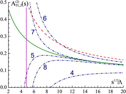
Figure 6: Two–loop timelike effective expansion function of the second order $A^{(2)}_{\text{\tiny TL},2}(s)$ [Eq. (6), solid curve] and the approximations corresponding to various orders of its re–expansion (6). The result of “naive” continuation (12) [the first term on the right–hand side of Eq. (6)] is shown by dashed curve. Numerical label next to a dot–dashed curve indicates the highest absolute value of power of $\ln w$ retained on the right–hand side of Eq. (6). The plotted functions are scaled by the factor of $10$. Vertical solid line marks the boundary of convergence range of the re–expansion (6) at $\sqrt{s}/\Lambda=\exp(\pi/2)\simeq 4.81$.

In turn, at the three–loop level the first–order function (76) takes the form

$$A^{(3)}_{\text{\scriptsize TL},1}(s) =A^{(2)}_{\text{\scriptsize TL},1}(s)-\frac{B_{1}^{2}}{\left(\ln^{2}w+\pi^{2}\right)^{\!\!2}}\Bigl{[}T_{1}(s)T_{2}(s)+\ln w\Bigr{]}+$$

$$+\frac{B_{2}\ln w}{\left(\ln^{2}w+\pi^{2}\right)^{\!\!2}},$$ (81)

where $A^{(2)}_{\text{\scriptsize TL},1}(s)$ is specified in Eq. (78) and

$$T_{1}(s) =a^{(1)}_{\text{\scriptsize{TL}}}(s)\,\ln w-W(s),$$ (82)

$$T_{2}(s) =\pi^{2}a^{(1)}_{\text{\scriptsize{TL}}}(s)+W(s)\,\ln w.$$ (83)

As for the four–loop first–order function (76), it can be represented as

$$A^{(4)}_{\text{\scriptsize TL},1}(s) =A^{(3)}_{\text{\scriptsize TL},1}(s)+\frac{1}{\left(\ln^{2}w+\pi^{2}\right)^{\!\!3}}\frac{B_{3}}{2}\!\left(\ln^{2}w-\frac{\pi^{2}}{3}\right)+$$

$$+\frac{B_{1}B_{2}}{\left(\ln^{2}w+\pi^{2}\right)^{\!\!3}}\!\biggl{\{}\frac{\pi^{2}}{3}-3T_{2}(s)\ln w+\pi^{2}W(s)+$$

$$+\ln^{2}w\Bigl{[}a^{(1)}_{\text{\scriptsize{TL}}}(s)\ln w-1\!\Bigr{]}\!\!\biggr{\}}-\frac{1}{\left(\ln^{2}w+\pi^{2}\right)^{\!\!3}}\frac{B_{1}^{3}}{2}\times$$

$$\times\!\!\Biggl{\{}\!2T_{2}(s)\ln w\Bigl{[}W(s)-3\Bigr{]}-T_{2}^{2}(s)\!\Bigl{[}2T_{1}(s)+1\Bigr{]}\!+$$

$$+\pi^{2}T_{1}^{2}(s)\biggl{[}\frac{2}{3}T_{1}(s)+3\biggr{]}+\ln^{2}w\Bigl{[}2\,a^{(1)}_{\text{\scriptsize{TL}}}(s)\ln w-1\Bigr{]}+$$

$$+2W^{2}(s)\ln^{2}w\Bigl{[}T_{1}(s)+W(s)-2\Bigr{]}+\frac{\pi^{2}}{3}+$$

$$+2W(s)\Bigl{[}1-W(s)\Bigr{]}\!\!\Bigl{[}\pi^{2}+a^{(1)}_{\text{\scriptsize{TL}}}(s)\ln^{3}w\Bigr{]}\!\!\Biggr{\}},$$ (84)

where the functions $A^{(3)}_{\text{\scriptsize TL},1}(s)$, $W(s)$, $T_{1}(s)$, and $T_{2}(s)$ are given by Eqs. (6), (80), (82), and (83), respectively. It is worthwhile to note also that the functions $A^{(\ell)}_{\text{\scriptsize TL},j}(s)$ (76) entering Eq. (75) can be computed numerically by making use of the routines included in the freely available program packages QCDDPT1 [which, being based on a less universal method of calculation of the relevant spectral function (11) than that of Eq. (5), is applicable at first four loop levels only] and QCDDPT2 .

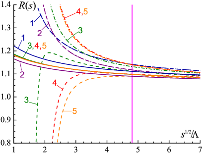
Figure 7: The function $R^{(\ell)}(s)$ [Eq. (10), solid curves], its naive form [Eq. (12), dot–dashed curves], and the re–expanded approximation [Eq. (31), dashed curves] at various loop levels ($1\leq\ell\leq 5$). Vertical solid line marks the boundary of convergence range of the re–expansion (31) at $\sqrt{s}/\Lambda=\exp(\pi/2)\simeq 4.81$. Numerical labels specify the loop level.

As discussed earlier, the $\pi^{2}$–terms play a valuable role in the studies of the strong interaction processes in the timelike domain, and their ignorance (complete or partial) may yield misleading results. In particular, this issue is illustrated by Fig. 6, which displays the two–loop timelike effective expansion function of the second order $A^{(2)}_{\text{\scriptsize TL},2}(s)$ [Eq. (6), solid curve] and the approximations (dashed and dot–dashed curves) corresponding to various orders of its re–expansion for $\sqrt{s}/\Lambda>\exp(\pi/2)\simeq 4.81$:

$$A^{(2)}_{\text{\scriptsize TL},2}(s) \simeq\left[a^{(2)}_{\text{s}}(|s|)\right]^{2}\!\!-\frac{\pi^{2}}{\ln^{4}w}+\frac{\pi^{2}}{\ln^{5}w}\,B_{1}\!\!\left(\!4\ln\ln w-\frac{7}{3}\right)\!-$$

$$-\frac{\pi^{2}}{\ln^{6}w}\!\left[\frac{B_{1}^{2}}{3}\Bigl{(}\!10\ln^{2}\ln w-9\ln\ln w+1\!\Bigr{)}\!-\pi^{2}\right]\!-$$

$$-\frac{\pi^{4}}{\ln^{7}w}\frac{3B_{1}}{10}\Bigl{(}20\ln\ln w-19\Bigr{)}\!+\mathcal{O}\!\left(\frac{1}{\ln^{8}w}\right)\!\!.$$ (85)

Specifically, the dashed curve shows the result of naive continuation of the respective term of the Adler function perturbative expansion into the timelike domain (12) [the first term on the right–hand side of Eq. (6)], whereas the dot–dashed curves additionally include the lowest–order $\pi^{2}$–terms [numerical labels indicate the highest absolute value of power of $\ln w$ retained in Eq. (6)]. Figure 6 implies that the re–expansion (6) converges rather slowly at low and moderate energies. Furthermore, even at relatively high energies $A^{(2)}_{\text{\scriptsize TL},2}(s)$ (6) considerably differs from $\bigl{[}a^{(2)}_{\text{s}}(|s|)\bigr{]}^{2}$, the latter being the only part of the function (6), which is retained in the two–loop approximation of the $R$–ratio (31). For example, as one can infer from Fig. 6, for $\sqrt{s}/\Lambda=20$ the function $\bigl{[}a^{(2)}_{\text{s}}(|s|)\bigr{]}^{2}$ exceeds $A^{(2)}_{\text{\scriptsize TL},2}(s)$ by about $21\,\%$, and to securely achieve $10\,\%$ accuracy in the re–expansion (6) the inclusion of the $\pi^{2}$–terms up to the order of $\ln^{-7}w$ is required.

The issue of the higher–loop stability of the $R$–ratio of electron–positron annihilation into hadrons is also elucidated by Fig. 7. In particular, this Figure displays the proper expression $R^{(\ell)}(s)$ [Eq. (10), solid curves], its naive form $R^{(\ell)}_{\text{naive}}(s)$ [Eq. (12), dot–dashed curves], and the truncated re–expanded approximation $R^{(\ell)}_{\text{appr}}(s)$ [Eq. (31), dashed curves] at various loop levels ($1\leq\ell\leq 5$). Figure 7 makes it evident that the loop convergence of the commonly employed approximation $R^{(\ell)}_{\text{appr}}(s)$ (31) is worse than that of both the proper expression $R^{(\ell)}(s)$ (10) and the naive one $R^{(\ell)}_{\text{naive}}(s)$ (12). As discussed earlier, this is primarily caused by the fact that the convergence range of the re–expanded approximation (31) is strictly limited to $\sqrt{s}/\Lambda>\exp(\pi/2)\simeq 4.81$, that, in turn, results in rather large values of the higher–order coefficients $\delta_{j}$ (32) embodying the contributions of the corresponding $\pi^{2}$–terms (4). In particular, as one can infer from Fig. 7, beyond the two–loop level (i.e., for $\ell\geq 3$) the curves corresponding to $R^{(\ell)}(s)$ (10) are nearly indistinguishable from each other, whereas the curves corresponding to $R^{(\ell)}_{\text{appr}}(s)$ (31) start to swerve quite above the boundary of its convergence range. For example, at $\sqrt{s}/\Lambda=2\exp(\pi/2)\simeq 9.62$ the relative difference between the $\ell$–loop and $(\ell+1)$–loop strong corrections to the proper expression $R^{(\ell)}(s)$ (10) is $0.4\,\%$ for $\ell=3$ and $0.003\,\%$ for $\ell=4$, whereas for the case of the commonly employed approximation $R^{(\ell)}_{\text{appr}}(s)$ (31) these values increase up to $4.4\,\%$ for $\ell=3$ and $2.5\,\%$ for $\ell=4$.

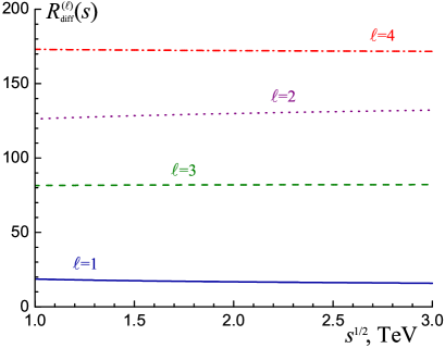
Figure 8: The function $R^{(\ell)}_{\text{\tiny{\text{diff}}}}(s)$ (86) in the energy range planned for the future CLIC experiment CLIC at various loop levels.

To expound the accuracy of approximation of the $R$–ratio (10) by its truncated re–expansion $R^{(\ell)}_{\text{appr}}(s)$ (31), it is worthwhile to mention also the following. At a moderate energy scale of the mass of $\tau$ lepton $\sqrt{s}=M_{\tau}$ the relative difference between the $\ell$–loop strong corrections $r^{(\ell)}(s)$ (10) and $r^{(\ell)}_{\text{appr}}(s)$ (31) turns out to be as high as $26\,\%$, $28\,\%$, $14\,\%$, $2\,\%$, and $7\,\%$ at the one–, two–, three–, four–, and five–loop levels, respectively. Moreover, it appears that even at high energies the ignorance of the higher–order $\pi^{2}$–terms in the truncated re–expanded approximation (31) may produce a considerable effect. In particular, this issue is illustrated by Fig. 8, which displays the quantity

$$R^{(\ell)}_{\text{diff}}(s)=\left|\frac{R^{(\ell)}_{\text{appr}}(s)-R^{(\ell)}(s)}{R^{(\ell)}_{\text{appr}}(s)-R^{(\ell+1)}_{\text{appr}}\!(s)}\right|\!\times\!100\,\%$$ (86)

at various loop levels. Specifically, as one can infer from Fig. 8, in the energy range planned for the future CLIC experiment CLIC the effect of inclusion of the $\pi^{2}$–terms discarded in the approximate expression $R^{(\ell)}_{\text{appr}}(s)$ (31) is either comparable to or prevailing over the effect of inclusion of the next–order perturbative correction.

7 Conclusions

The strong corrections to the $R$–ratio of electron–positron annihilation into hadrons are studied at the higher–loop levels. In particular, the derivation of a general form of the commonly employed approximate expression for the $R$–ratio (which constitutes its truncated re–expansion at high energies) is delineated, the appearance of the pertinent $\pi^{2}$–terms is expounded, and their basic features are examined. It is demonstrated that the validity range of such approximation is strictly limited to $\sqrt{s}/\Lambda>\exp(\pi/2)\simeq 4.81$ and that it converges rather slowly when the energy scale approaches this value. The spectral function required for the proper calculation of the $R$–ratio is explicitly derived and its properties at the higher–loop levels are studied. The developed method of calculation of the spectral function enables one to obtain the explicit expression for the latter at an arbitrary loop level. By making use of the derived spectral function the proper expression for the $R$–ratio is calculated up to the five–loop level and its properties are examined. In particular, it is shown that the loop convergence of the proper expression for the $R$–ratio is better than that of its commonly employed approximation and that the omitted higher–order $\pi^{2}$–terms in the latter may produce a considerable effect.

- (1) D. d’Enterria et al., arXiv:1512.05194 [hep-ph].
- (2) CEPC–SPPC Study Group, Report IHEP–CEPC–DR–2015–01 (2015).
- (3) H. Baer et al., arXiv:1306.6352 [hep-ph].
- (4) M. Aicheler et al., Report CERN–2012–007 (2012).
- (5) J. Grange et al. [Muon g–2 Collaboration], arXiv:1501.06858 [physics.ins-det].
- (6) M. Otani [E34 Collaboration], JPS Conf. Proc. 8, 025008 (2015).
- (7) R.P. Feynman, Photon–hadron interactions, Benjamin, Massachusetts, 282 p. (1972).
- (8) S.L. Adler, Phys. Rev. D 10, 3714 (1974).
- (9) A.V. Radyushkin, report JINR E2–82–159 (1982); JINR Rapid Commun. 78, 96 (1996); arXiv:hep-ph/9907228.
- (10) N.V. Krasnikov and A.A. Pivovarov, Phys. Lett. B 116, 168 (1982).
- (11) A.A. Pivovarov, Nuovo Cim. A 105, 813 (1992).
- (12) F. Guerrero and A. Pich, Phys. Lett. B 412, 382 (1997); A. Pich and J. Portoles, Phys. Rev. D 63, 093005 (2001); D. Gomez Dumm and P. Roig, Eur. Phys. J. C 73, 2528 (2013); P. Roig, A. Guevara, and G. Lopez Castro, Phys. Rev. D 89, 073016 (2014).
- (13) V. Bernard and E. Passemar, Phys. Lett. B 661, 95 (2008); V. Bernard, M. Oertel, E. Passemar, and J. Stern, Phys. Rev. D 80, 034034 (2009); G. Colangelo, E. Passemar, and P. Stoffer, Eur. Phys. J. C 75, 172 (2015); J. Phys. Conf. Ser. 800, 012026 (2017).
- (14) R. Garcia–Martin, R. Kaminski, J.R. Pelaez, and J. Ruiz de Elvira, Phys. Rev. Lett. 107, 072001 (2011); R. Garcia–Martin, R. Kaminski, J.R. Pelaez, J. Ruiz de Elvira, and F.J. Yndurain, Phys. Rev. D 83, 074004 (2011); S. Dubnicka, A.Z. Dubnickova, R. Kaminski, and A. Liptaj, ibid. 94, 054036 (2016); P. Bydzovsky, R. Kaminski, and V. Nazari, ibid. 94, 116013 (2016).
- (15) G. Colangelo, M. Hoferichter, A. Nyffeler, M. Passera, and P. Stoffer, Phys. Lett. B 735, 90 (2014); G. Colangelo, M. Hoferichter, B. Kubis, M. Procura, and P. Stoffer, ibid. 738, 6 (2014); G. Colangelo, M. Hoferichter, M. Procura, and P. Stoffer, JHEP 1409, 091 (2014); 1509, 074 (2015); 1704, 161 (2017); Phys. Rev. Lett. 118, 232001 (2017).
- (16) A.V. Nesterenko, Strong interactions in spacelike and timelike domains: Dispersive approach, Elsevier, Amsterdam, 222 p. (2017).
- (17) A.V. Nesterenko and J. Papavassiliou, J. Phys. G 32, 1025 (2006).
- (18) A.V. Nesterenko, Phys. Rev. D 88, 056009 (2013); J. Phys. G 42, 085004 (2015).
- (19) A.V. Nesterenko and J. Papavassiliou, Phys. Rev. D 71, 016009 (2005); Int. J. Mod. Phys. A 20, 4622 (2005); Nucl. Phys. B (Proc. Suppl.) 152, 47 (2005); 164, 304 (2007).
- (20) P.A. Baikov, K.G. Chetyrkin, and J.H. Kuhn, Phys. Rev. Lett. 101, 012002 (2008); 104, 132004 (2010); P.A. Baikov, K.G. Chetyrkin, J.H. Kuhn, and J. Rittinger, Phys. Lett. B 714, 62 (2012).
- (21) A.L. Kataev and V.V. Starshenko, Mod. Phys. Lett. A 10, 235 (1995).
- (22) P.A. Baikov, K.G. Chetyrkin, and J.H. Kuhn, Phys. Rev. Lett. 118, 082002 (2017); F. Herzog, B. Ruijl, T. Ueda, J.A.M. Vermaseren, and A. Vogt, JHEP 1702, 090 (2017).
- (23) A.V. Nesterenko, Nucl. Phys. B (Proc. Suppl.) 186, 207 (2009); 234, 199 (2013); Nucl. Part. Phys. Proc. 258, 177 (2015); 270, 206 (2016).
- (24) A.V. Nesterenko, SLAC eConf C0706044, 25 (2008); C1106064, 23 (2011).
- (25) A.V. Nesterenko, PoS ConfinementX, 350 (2012); AIP Conf. Proc. 1701, 040016 (2016); EPJ Web Conf. 137, 05021 (2017).
- (26) K.A. Milton and I.L. Solovtsov, Phys. Rev. D 55, 5295 (1997); Phys. Rev. D 59, 107701 (1999).
- (27) D.V. Shirkov and I.L. Solovtsov, Phys. Rev. Lett. 79, 1209 (1997); Theor. Math. Phys. 150, 132 (2007).
- (28) G. Cvetic and C. Valenzuela, Phys. Rev. D 74, 114030 (2006); 84, 019902(E) (2011); Braz. J. Phys. 38, 371 (2008); G. Cvetic and A.V. Kotikov, J. Phys. G 39, 065005 (2012); A.P. Bakulev, Phys. Part. Nucl. 40, 715 (2009); N.G. Stefanis, ibid. 44, 494 (2013).
- (29) G. Cvetic, A.Y. Illarionov, B.A. Kniehl, and A.V. Kotikov, Phys. Lett. B 679, 350 (2009); A.V. Kotikov, PoS (Baldin ISHEPP XXI), 033 (2013); PoS (Baldin ISHEPP XXII), 028 (2015); A.V. Kotikov and B.G. Shaikhatdenov, Phys. Part. Nucl. 44, 543 (2013); Phys. Atom. Nucl. 78, 525 (2015); A.V. Kotikov, V.G. Krivokhizhin, and B.G. Shaikhatdenov, J. Phys. G 42, 095004 (2015); A.V. Kotikov, B.G. Shaikhatdenov, and P. Zhang, arXiv:1706.01849 [hep-ph]; C. Ayala, G. Cvetic, A.V. Kotikov, and B.G. Shaikhatdenov, arXiv:1708.06284 [hep-ph].
- (30) G. Cvetic and C. Villavicencio, Phys. Rev. D 86, 116001 (2012); C. Ayala and G. Cvetic, ibid. 87, 054008 (2013); P. Allendes, C. Ayala, and G. Cvetic, ibid. 89, 054016 (2014); C. Ayala, G. Cvetic, and R. Kogerler, J. Phys. G 44, 075001 (2017); C. Ayala, G. Cvetic, R. Kogerler, and I. Kondrashuk, arXiv:1703.01321 [hep-ph]; C. Ayala, arXiv:1710.00255 [hep-ph]; G. Cvetic, arXiv:1712.00622 [hep-ph].
- (31) M. Baldicchi and G.M. Prosperi, Phys. Rev. D 66, 074008 (2002); AIP Conf. Proc. 756, 152 (2005); M. Baldicchi, G.M. Prosperi, and C. Simolo, ibid. 892, 340 (2007); M. Baldicchi, A.V. Nesterenko, G.M. Prosperi, D.V. Shirkov, and C. Simolo, Phys. Rev. Lett. 99, 242001 (2007); M. Baldicchi, A.V. Nesterenko, G.M. Prosperi, and C. Simolo, Phys. Rev. D 77, 034013 (2008).
- (32) N. Christiansen, M. Haas, J.M. Pawlowski, and N. Strodthoff, Phys. Rev. Lett. 115, 112002 (2015); N. Mueller and J.M. Pawlowski, Phys. Rev. D 91, 116010 (2015); R. Lang, N. Kaiser, and W. Weise, Eur. Phys. J. A 51, 127 (2015).
- (33) K.A. Milton, I.L. Solovtsov, and O.P. Solovtsova, Phys. Lett. B 439, 421 (1998); Phys. Rev. D 60, 016001 (1999); R.S. Pasechnik, D.V. Shirkov, and O.V. Teryaev, ibid. 78, 071902 (2008); R.S. Pasechnik, J. Soffer, and O.V. Teryaev, ibid. 82, 076007 (2010).
- (34) K.A. Milton, I.L. Solovtsov, and O.P. Solovtsova, Phys. Lett. B 415, 104 (1997); K.A. Milton, I.L. Solovtsov, O.P. Solovtsova, and V.I. Yasnov, Eur. Phys. J. C 14, 495 (2000).
- (35) G. Ganbold, Phys. Rev. D 79, 034034 (2009); 81, 094008 (2010); PoS (Confinement X), 065 (2012).
- (36) A. Bakulev, K. Passek–Kumericki, W. Schroers, and N. Stefanis, Phys. Rev. D 70, 033014 (2004); 70, 079906(E) (2004); A. Bakulev, A. Pimikov, and N. Stefanis, ibid. 79, 093010 (2009); N. Stefanis, Nucl. Phys. B (Proc. Suppl.) 152, 245 (2006).
- (37) N.G. Stefanis, W. Schroers, and H.C. Kim, Phys. Lett. B 449, 299 (1999); Eur. Phys. J. C 18, 137 (2000); A.I. Karanikas and N.G. Stefanis, Phys. Lett. B 504, 225 (2001); 636, 330(E) (2006); A.P. Bakulev, A.V. Radyushkin, and N.G. Stefanis, Phys. Rev. D 62, 113001 (2000); A.P. Bakulev, A.I. Karanikas, and N.G. Stefanis, ibid. 72, 074015 (2005).
- (38) G. Cvetic, R. Kogerler, and C. Valenzuela, Phys. Rev. D 82, 114004 (2010); J. Phys. G 37, 075001 (2010); G. Cvetic and R. Kogerler, Phys. Rev. D 84, 056005 (2011).
- (39) O. Teryaev, Nucl. Phys. B (Proc. Suppl.) 245, 195 (2013); A.V. Sidorov and O.P. Solovtsova, Nonlin. Phenom. Complex Syst. 16, 397 (2013); Mod. Phys. Lett. A 29, 1450194 (2014); J. Phys. Conf. Ser. 678, 012042 (2016); Phys. Part. Nucl. Lett. 14, 1 (2017).
- (40) A.V. Nesterenko, Phys. Rev. D 62, 094028 (2000); 64, 116009 (2001).
- (41) A.V. Nesterenko, Int. J. Mod. Phys. A 18, 5475 (2003); Nucl. Phys. B (Proc. Suppl.) 133, 59 (2004).
- (42) A.V. Nesterenko, Mod. Phys. Lett. A 15, 2401 (2000); A.V. Nesterenko and I.L. Solovtsov, ibid. 16, 2517 (2001).
- (43) A.C. Aguilar, A.V. Nesterenko, and J. Papavassiliou, J. Phys. G 31, 997 (2005); Nucl. Phys. B (Proc. Suppl.) 164, 300 (2007).
- (44) C. Contreras, G. Cvetic, O. Espinosa, and H.E. Martinez, Phys. Rev. D 82, 074005 (2010); C. Ayala, C. Contreras, and G. Cvetic, ibid. 85, 114043 (2012).
- (45) R.G. Moorhouse, M.R. Pennington, and G.G. Ross, Nucl. Phys. B 124, 285 (1977); M.R. Pennington, R.G. Roberts, and G.G. Ross, ibid. 242, 69 (1984); M.R. Pennington and G.G. Ross, Phys. Lett. B 102, 167 (1981).
- (46) J.D. Bjorken, report SLAC–PUB–5103 (1989).
- (47) G.M. Prosperi, M. Raciti, and C. Simolo, Prog. Part. Nucl. Phys. 58, 387 (2007).
- (48) B. Schrempp and F. Schrempp, Z. Phys. C 6, 7 (1980).
- (49) A.V. Nesterenko and S.A. Popov, Nucl. Part. Phys. Proc. 282, 158 (2017).
- (50) A.V. Nesterenko and C. Simolo, Comput. Phys. Commun. 181, 1769 (2010); 182, 2303 (2011).
- (51) A.V. Nesterenko and C. Simolo, in preparation.