Dynamic SPECT reconstruction with temporal edge correlation

Abstract

In dynamic imaging, a key challenge is to reconstruct image sequences with high temporal resolution from strong undersampling projections due to a relatively slow data acquisition speed. In this paper, we propose a variational model using the infimal convolution of Bregman distance with respect to total variation to model edge dependence of sequential frames. The proposed model is solved via an alternating iterative scheme, for which each subproblem is convex and can be solved by existing algorithms. The proposed model is formulated under both Gaussian and Poisson noise assumption and the simulation on two sets of dynamic images shows the advantage of the proposed method compared to previous methods.
Keywords: Dynamic SPECT;  Sparsity;  Low rank representation ;  Infimal convolution; Bregman distance.

• May 2017

1 Introduction

Single Photon Emission Computed Tomography (SPECT) and Positron emission tomography (PET)[1, 2, 3, 4] are nuclear medical imaging modalities that detect the trace concentrations of radioactively labeled pharmaceutical injected in the body within chosen volumes of interest. After an isotope tagged to a biochemical compound is injected into a patient s vein, the biochemical compound travels to body organs (liver, kidney, brain, heart and the peripheral vascular system) through the blood stream, and is absorbed by these organs according to their affinity for the particular compound [5, 6]. The SPECT system, usually consisting of one, two or three detector head(s)[7, 8, 9], can record radiopharmaceutical exchange between biological compartments and isotope decay in the patient s body as the detector(s) rotate around the body.

As very few views can be obtained in one time interval, dynamic SPECT reconstruction is an ill-posed inverse problem with incomplete noisy data. On assuming that motion and deformation are negligible during the data acquiring procedure, we aim to reconstruct the dynamic radioiostrope distribution with high temporal resolution. In fact, it is crucial to extract the actual decay of the isotope, i.e. time activity curves (TACs) of different organ compartments [10] [11], either from projections or reconstructed images [12, 11, 5, 13, 14, 15, 16, 17].

Besides methods that reconstruct each frame of dynamic sequence independently [18, 19], many approaches [7, 20, 21, 22] have been proposed to monitor the tracer concentrations over time, under the assumption of static radioactivity concentration during the acquisition period. However, as the measuring procedure usually takes a considerable amount of time, physiological processes in the body are dynamic and some organs (kidney, heart) show a significant change of activity. Hence, ignoring the dynamics of radioisotopes over the acquisition and applying the conventional tomographic reconstruction method (such as filtered back projection method (FBP)) yields inaccurate reconstructions with serious artifacts. Joint reconstruction approaches for dynamic imaging were proposed in [23, 24], where dynamic images of the different time are treated collectively through motion compensation and temporal basis function. Then, the dynamic processes of blood flow, tissue perfusion and metabolism can be described by tracer kinetic modeling [5]. For example, a spatial segmentation and temporal B-Splines were combined to reconstruct spatiotemporal distributions from projection data [reutter2000direct, 14]. In a different form, dynamic SPECT images are represented by low-rank factorization models in [25, 26], and further constraints are enforced for the representation coefficients and basis. In some recent work, motion of the organs has been taken into account for the dynamic CT reconstruction in [27, 28, 29, 30, 31, 32, 33].

In this paper, we propose a new variational model in which we take local and global coherence in temporal-spatial domain into consideration. The key idea is that dynamic image sequences possess similar structures of radioactivity concentrations. In fact, the boundary of organs, which are the locations with large gradient, are preserved or changed mildly along time. Inspired by color Bregman TV for color image reconstruction [34] and PET-MRI joint reconstruction [35], we introduce the infimal convolution of Bregman distance with respect to total variation as a regularization, to obtain the dependence of edges of sequential images. Furthermore, based on our previous work [25, 26], low rank matrix approximation $U=\alpha B^{T}$ is demonstrated to be a robust representation for dynamic images, especially with proper regularization on the coefficient $\alpha$ and the basis $B$ that corresponds to the TACs of different compartments. Specially, the group sparsity on the coefficient $\alpha$ is enforced as the concentration distribution is mixed from few basis elements for each voxel. Finally, the proposed variational model is composed of a data fidelity term and several regularization elements, to overcome the incompleteness and ill-posedness of the reconstruction problem.

The proposed model is solved alternatingly, with each subproblems can be solved with popular operator splitting methods at ease. In particular, the primal-dual hybrid gradient (PDHG) algorithm [36, 37, 38] is applied to solve the subproblem for the images $U$ and Proximal Forward-Backward Spliting (PFBS) for the coefficients $\alpha$ and the basis $B$. Our numerical experiments on simulated phantom shows the feasibility of the proposed model for reconstruction from highly undersampled data with noise, compared to conventional methods such as FBP method and least square methods (or EM). Monte-Carlo simulation of noisy data is also performed to demonstrate the robustness of the proposed model on two phantom images.

The paper is organized as followed: Section 2 presents the proposed model, where section 2.2 briefly introduces the concept of infimal convolution of Bregman distance and models the edge alignments of images by infimal convolution and section 2.3 models the spatiotemporal property of dynamic image. Section 3 describe the numerical algorithm. Finally, Section 4 demonstrates numerical results on simulated dynamic images, in the settings of Gaussian, Poisson noise and Monte Carlo simulation.

2 Model

The regularization of our proposed variational model is based on some properties of dynamic SPECT images. First of all, dynamic image sequences are originated from the radioactivity concentration of few compartments in the field of view. Thus we can naturally use a low rank matrix factorization representation for the image, with the basis related to the time activity curves, which are usually smooth, and the coefficients are related to the locations of the organs that are piecewise constant. For the scenario of large motion, such as the case of cardiac and respiratory dynamic imaging, a proper modeling of motion correction is necessary for a reconstruction with high accuracy. In this paper, we assume that the body movement is minor which means the boundaries of organs of image sequence are almost static and aim to capture the activity decay in each region. One can incorporate a registration or motion correction process in the model for the extension to the case of large motion. In other words, the edges of the image sequence share the similar locations. We will then use the tool of infimal convolution of the Bregman distance with respect to total variation to enforce edge alignments. In the following, we will present the regularization terms in details.

2.1 Observation model

In dynamic SPECT, the goal is to reconstruct a spatiotemporal radioiostrope distribution $u_{t}(x)$ for $x\in\Omega\subset\mathcal{R}^{2}$ in a given time interval. Given a sequence of projection data $f_{1},f_{2},\cdots f_{T}$ with different view angles, we aim to reconstruct the samples of continuous image $u_{t}(x)$ at $t$-th time interval, i.e. the image sequence $u_{1}(x),u_{2}(x),\cdots u_{T}(x)$. If we denote $A_{1},A_{2},\cdots A_{T}$ as $T$ corresponding projection matrices, the observation model can be described as

$$A_{t}u_{t}=f_{t},\qquad t=1,2,\cdots,T.$$

For ease of notations, we present the discrete form of $u_{t}(x)$ with $M$ pixel/voxel at each frame, and the dynamic image is represented as $U\in\mathbb{R}^{M\times T}$. The sequence of projections are formulated in linear form:

$$\mathcal{A}U=f$$ (1)

where $\mathcal{A}U=(A_{1}u_{1},A_{2}u_{2},\cdots A_{T}u_{T})$, and $f=(f_{1},f_{2},\cdots f_{T})$. In practice, the observed projection data often inevitably accompany with noise. If white Gaussian noise is considered, i.e.

$$\mathcal{A}U+N(0,\sigma^{2})=f.$$

The negative log likelihood functional leads to

$$H(f,\mathcal{A}U)=\frac{1}{2}\sum_{i=1}^{T}\|A_{i}u_{i}-f_{i}\|_{2}^{2}\triangleq\frac{1}{2}\|\mathcal{A}U-f\|_{F}^{2}.$$ (2)

Similarily, if Poisson noise is considered, this term can be replaced by the log likelihood

$$H(f,\mathcal{A}U)=D_{\mathrm{KL}}(f,\mathcal{A}U)$$

$$=\sum_{i=1}^{T}\bigg{(}\langle A_{i}u_{i},\mathrm{1}\rangle-\langle f_{i},\log{(A_{i}u_{i})}\rangle\bigg{)}\triangleq\langle\mathcal{A}U,\mathrm{1}\rangle-\langle f,\log{(\mathcal{A}U)}\rangle.$$ (3)

2.2 Edge alignments

For any two nonzero vectors $\vec{p},\vec{q}\in\mathcal{R}^{2}$, we first define a relative distance measure

$$d(\vec{p},\vec{q}):=\frac{\|\vec{p}\|\|\vec{q}\|-\vec{p}\cdot\vec{q}}{\|\vec{q}\|}=\|\vec{p}\|(1-\frac{\vec{p}}{\|\vec{p}\|}\cdot\frac{\vec{q}}{\|q\|})$$ (4)

where $\cdot$ is the standard dot product on $\mathcal{R}^{d}$, $\|\vec{p}\|$ denotes Euclidian norm. It is easy to see that if and only if $\vec{p}$ and $\vec{q}$ are parallel and point to the same direction, $d(\vec{p},\vec{q})=0$. In order to avoid penalizing the opposite direction, one can define a ”symmetric” distance as

$$\mathcal{D}(\vec{p},\vec{q}):=\frac{\|\vec{p}\|\|\vec{q}\|-|\vec{p}\cdot\vec{q}|}{\|\vec{q}\|}=\|\vec{p}\|(1-|\frac{\vec{p}}{\|\vec{p}\|}\cdot\frac{\vec{q}}{\|\vec{q}\|}|).$$ (5)

For two given images $u$ and $v$, we are interested in measuring the degree of parallelism of the gradients at each pixel as a correlation criterion of two images. We first consider the Bregman distance with respect to the total variation of two images (in a continuous setting and assume that $\frac{\nabla u}{|\nabla u|}$ and $\frac{\nabla v}{|\nabla v|}$ are well defined a.e.):

$$D_{\mathrm{TV}}^{p}(u,v)=\int_{\Omega}|\nabla u|(1-\frac{\nabla u}{|\nabla u|}\cdot\frac{\nabla v}{|\nabla v|})=\int_{\Omega}d(\nabla u,\nabla v)$$

where $p=\nabla^{T}\frac{\nabla v}{\|\nabla v\|}\in\partial J(v)$ and the Bregman distance is defined as

$$D_{J}^{p}(u,v)=J(u)-J(v)-\langle p,u-v\rangle$$ (6)

for a convex and nonnegative functional. We can see that there is no penalty for aligned image gradients if the angle between $\frac{\nabla u}{|\nabla u|}$ and $\frac{\nabla v}{|\nabla v|}$ is zero, independent of the magnitude of the jump in $u$ and $v$.

To define a symmetric distance as in (5), the infimal convolution of the Bregman distance in [34] is introduced to gain independence of the direction of the gradient vector. The infimal convolution[39]) of two convex function $I,J:\mathcal{X}\rightarrow(-\infty,\infty]$ is defined as

$$I\Box J(x):=\inf_{z\in\mathcal{X}}\{I(x-z)+J(z)\}.$$

For example, if $p,q\in\mathcal{R}^{n}$, the infimal convolution between the $\ell^{1}$ Bregman distances $D^{s}_{\|\cdot\|_{1}}(p,q)$ and $D^{-s}_{\|\cdot\|_{1}}(p,-q)$ is given by

$$D^{s}_{\|\cdot\|_{1}}(p,q)\Box D^{-s}_{\|\cdot\|_{1}}(p,-q)=\sum_{i=1}^{n}|p_{i}|-|s_{i}p_{i}|$$

We can see that $D^{s}_{\|\cdot\|_{1}}(p,q)\Box D^{-s}_{\|\cdot\|_{1}}(p,-q)$ is zero if $|s(i)|=1$ for $|p_{i}|\neq 0$, thus the support of $p$ is contained in the support of $q$, no matter the sign of $p(i)$ and $q(i)$. Inspired of this, the regularization in the form of infimal convolution of Bregman distance with respect to total variation is considered as a measure of parallelism of the edges between two images:

$$R(u,v):=D_{TV}^{p}(u,v)\Box D_{TV}^{-p}(u,-v)$$ (7)

This formulation is originally proposed as color Bregman total variation in [34] to couple different channels of color images. Ehrhardt et al. [40][41][35] used the above derivation and the resulting measure for PET-MRI joint reconstruction. More rigourous definition in bounded variation space and geometric interpretation, one can refer to [34][35].

For the dynamic SPECT image, we consider the infimal convolution of the Bregman distance of the total variation to enforce the alignment of the edge sets of sequential frames. Specifically, let $u_{i}^{n}$ be the estimate of frame $i$ at iteration $n$, we consider an average of the deviation of next estimate to this image and the other frames $u_{1}^{n},u_{2}^{n},\cdots u_{i-1}^{n},u_{i+1}^{n},\cdots u_{T}^{n}$. That is,

$$R(u_{i})=w_{i,i}D_{\mathrm{TV}}^{p_{i}^{n}}(u_{i},u^{n}_{i})+\sum_{j=1,~{}j\neq i}^{T}w_{i,j}D_{\mathrm{TV}}^{p_{j}^{n}}(u_{i},u^{n}_{j})\square D_{\mathrm{TV}}^{-p_{j}^{n}}(u_{i},-u^{n}_{j})$$ (8)

where $\sum_{j=1}^{T}w_{i,j}=1.$

2.3 Low rank and sparse approximation

The compartment model is often used to describe the concentration change of the tracer in the dynamic image [42]. It is assumed that the transportation and mixture take places between the different physical compartments, such as organ and tissue. We impose the low-rank structure of the dynamic images by assuming that the unknown concentration distribution is a sparse linear combination of a few temporal basis functions which represent the TACs of different compartments. In other words, it assumes that concentration distribution of the radioisotope $u_{t}(x)$, for each pixel/voxel $x\in\Omega$ at time $t$ can be approximated as a linear combination of some basis TACs:

$$u_{t}(x)=\sum_{k=1}^{K}\alpha_{k}(x)B_{k}(t),$$ (9)

where $B_{k}(t)$ denotes the TAC for $k$-th compartment at time $t$, and $\alpha_{k}(x)$ denotes the mixed coefficients. This can be written in matrix form as

$$U=\alpha B^{T},$$

where $\alpha\in\mathbb{R}^{M\times K}$ and $B\in\mathbb{R}^{T\times K}$ with $K$ as the number of compartments. As in general $K$ is a small number compared to the number of time intervals $T$, we naturally obtain a low rank matrix representation for $U$.

Furthermore, $\alpha_{k}$ is the $k$-th column of the coefficient $\alpha$, and each element of $\alpha_{k}$ represents the contribution of the $k$-th basis to the current pixel. For the image only have few compartments, the nonzero coefficients in $\alpha$ is sparse. In temporal direction, we want to use the least number of bases, that is, as many columns of $\alpha$ as possible are entirely zero. We can use $\ell_{1,\infty}$ to describe this quantity

$$\|\alpha\|_{1,\infty}=\sum_{j=1}^{K}\max_{i}|\alpha_{i,j}|.$$

This term is designed to select few number of basis to represent the images $u_{t}$. This type of column sparsity was previously studied in [43] and in [44] for hyperspectral image classification.

Finally, to enfore the smoothness of the decay of radioactive distribution, we also use

$$\|\partial_{t}U\|^{2}_{2}=\sum_{m=1}^{M}\sum_{t=1}^{T}(u_{t+1}(m)-u_{t}(m))^{2}$$

as another regularization.

Now, we summarize the model that we propose for the reconstruction of dynamic images. Given an estimate of $U^{n}$ at step $n$, we propose to solve the following reconstruction model

$$\min_{U\geq 0,\alpha,B}H(f,\mathcal{A}U)+\frac{\gamma}{2}\|U-\alpha B^{T}\|_{2}^{2}+\beta\|\alpha\|_{1,\infty}+\frac{\eta}{2}\|\partial_{t}U\|_{2}^{2}+\lambda\sum_{i=1}^{T}R(u_{i}),$$ (10)

where $\sum_{j=1}^{T}w_{i,j}=1,i=1,2\cdots T$, $\gamma,\beta,\eta,\lambda>0$ and $R(u_{i})$ is defined in (8).

The combination of multi regularization aims to take into account the spatial-temporal factorization with the constraints on the basis and the sparsity of representation coefficients, and the alignments of edges. We will show that the proposed model is robust for overcoming the incompleteness of projection data and noise.

3 Numerical algorithms

There are three variables $U,\alpha$ and $B$ in the proposed model (10), and non-smooth and complex regularization terms are involved. Thus it is a rather complex problem to solve directly for the three variables. We propose to solve the nonconvex optimization problem with alternating scheme on updating the image $U$, the coefficient $\alpha$ and the basis $B$.

In the following, we present the alternating algorithm that solves (10) with $H(f,\mathcal{A}U)$ is defined as (2.1).

$$U^{n+1}=\arg\min_{U\geq 0}H(f,\mathcal{A}U)+\frac{\gamma}{2}\|U-\alpha^{n}({B^{n}})^{T}\|_{2}^{2}+\frac{\eta}{2}\|\partial_{t}U\|_{2}^{2}+\lambda\sum_{i=1}^{T}R(u_{i}),$$

(11)

$$\alpha^{n+1}=\arg\min_{\alpha}\beta\|\alpha\|_{1,\infty}+\frac{\gamma}{2}\|U^{n}-\alpha(B^{n})^{T}\|_{2}^{2},$$ (12)

$$B^{n+1}=\arg\min_{B}\frac{\gamma}{2}\|U^{n+1}-\alpha^{n+1}B^{T}\|_{2}^{2}.$$ (13)

• In the subproblem (11), given $u_{i}^{n}$ and $p_{i}^{n}\in\partial J_{TV}(u_{i}^{n})$, $R(u_{i})$ can be rewritten as followed:

  $$R(u_{i}) =w_{i,i}\bigg{(}\mathrm{TV}(u_{i})-\langle p_{i}^{n},u_{i}\rangle\bigg{)}+\sum_{j=1,j\neq i}^{T}\inf_{z_{ij}}w_{i,j}\bigg{(}\mathrm{TV}(u_{i}-z_{ij})$$

  $$\quad-\langle p_{j}^{n},(u_{i}-z_{ij})\rangle+\mathrm{TV}(z_{ij})+\langle p_{j}^{n},z_{ij}\rangle\bigg{)}$$

  $$=w_{i,i}\bigg{(}\mathrm{TV}(u_{i})-\langle q_{i}^{n},\nabla u_{i}\rangle\bigg{)}+\sum_{j=1,j\neq i}^{T}\inf_{z_{ij}}w_{i,j}\bigg{(}\mathrm{TV}(u_{i}-z_{ij})$$

  $$\quad-\langle q_{j}^{n},\nabla(u_{i}-z_{ij})\rangle+\mathrm{TV}(z_{ij})+\langle q_{j}^{n},\nabla z_{ij}\rangle\bigg{)}$$

  $$\triangleq\inf_{\{z_{ij}\}_{j=1}^{T},j\neq i}\tilde{R}(u_{i},z_{i,\cdot}),$$

  where $\nabla^{T}q_{i}^{n}=p_{i}^{n},i=1,\cdots,T.$ Then, the subproblem (11) is reformulated as

  $$\min_{U\geq 0,Z}H(f,\mathcal{A}U)+\frac{\gamma}{2}\|U-\alpha^{n}({B^{n}})^{T}\|_{2}^{2}+\frac{\eta}{2}\|\nabla_{t}U\|_{2}^{2}+\lambda\sum_{i=1}^{T}\tilde{R}(u_{i},z_{i,\cdot}).$$ (15)

  We solve problem (15) by primal-dual hybrid gradient (PDHG) Algorithm [37, 38]. The problem formulation is as follows,

  $$\min_{X}\max_{Y}-F^{\ast}(Y)+G(X)+\langle\mathcal{K}X,Y\rangle,$$ (16)

  where $\mathcal{K}:\mathcal{U}\rightarrow\mathcal{V}$ is a linear and continuous operator between two finite dimensional vector spaces $\mathcal{U}$ and $\mathcal{V}$. $F:\mathcal{V}\rightarrow[0,+\infty]$ and $G:\mathcal{U}\rightarrow[0,+\infty]$ are proper, convex and lower semi-continuous functions. $F^{\ast}$ is the conjugate of $F$ and $\mathcal{W}^{\ast}=\mathcal{V}$. The PDHG iteration is,

  $$Y^{k+1}=(I+\sigma\partial F^{\ast})^{-1}(Y^{k}+\sigma\mathcal{K}\bar{X}^{k})$$ (17)

  $$X^{k+1}=(I+\tau\partial G)^{-1}(X^{k}-\tau\mathcal{K}^{\ast}Y^{k+1})$$ (18)

  $$\bar{X}^{k+1}=X^{k+1}+\theta(X^{k+1}-X^{k}).$$ (19)

  For our model, we have

  $$F(g,b,d_{ii},d_{ij}^{+},d_{ij}^{-}) :=H(f,g)+\frac{\eta}{2}\|b\|_{2}^{2}+\lambda\sum_{i=1}^{T}\Bigg{(}w_{i,i}\bigg{(}\|d_{ii}\|_{1}-\langle q_{i}^{n},d_{ii}\rangle\bigg{)}$$

  $$+\sum_{j=0,j\neq i}^{T}w_{i,j}\bigg{(}\|d^{+}_{ij}\|_{1}-\langle q_{j}^{n},d^{+}_{ij}\rangle+\|d^{-}_{ij}\|_{1}+\langle q_{j}^{n},d^{-}_{ij}\rangle\bigg{)}\Bigg{)},$$

  where $g=\mathcal{A}U;b=\partial_{t}U;d_{ii}=\nabla u_{i};d_{ij}^{+}=u_{i}-z_{ij};d_{ij}^{-}=\nabla z_{ij}$ and

  $$G(U):= \iota_{\{U\geq 0\}}(U)+\frac{\gamma}{2}\|U -\alpha^{n}(B^{n})^{T}\|_{2}^{2}.$$

  where $\iota_{\{U\geq 0\}}(U)$ is the characteristic function of the set $\{U\geq 0\}$. According to (• ‣ 3), we obtain the iterative scheme for each subproblem.

  • For the subproblem (17), the dual variables can be updated as

    $$g^{k+1}=\frac{\tilde{g}+1}{2}-\sqrt{(\frac{\tilde{g}+1}{2})^{2}+\sigma f-\tilde{g}},~{}~{}\tilde{g}=g^{k}+\sigma A\bar{U}^{k},$$

    $$b^{k+1}=\frac{\eta}{\eta+\sigma}\tilde{b},~{}~{}\tilde{b}=b^{k}+\sigma\partial_{t}\bar{U}^{k},$$

    $$(d_{ii})^{k+1}=w_{i,i}\Pi_{B^{\infty}_{(1)}}(\tilde{d}_{ii}/w_{i,i}-q^{n}_{i})+w_{i,i}q^{n}_{i},~{}~{}\tilde{d}_{ii}=(d_{ii})^{k}+\sigma\nabla\bar{u}_{i}^{k},$$

    $$(d^{+}_{ij})^{k+1}=w_{i,j}\Pi_{B^{\infty}_{(1)}}(\tilde{d}^{+}_{ij}/w_{i,j}-q^{n}_{j})+w_{i,j}q^{n}_{j},~{}~{}\tilde{d}^{+}_{ij}=(d^{+}_{ij})^{k}+\sigma\nabla(\bar{u}_{i}^{k}-\bar{z}^{k}_{ij}),$$

    $$(d^{-}_{ij})^{k+1}=w_{i,j}\Pi_{B^{\infty}_{(1)}}(\tilde{d}^{-}_{ij}/w_{i,j}+q^{n}_{j})-w_{i,j}q^{n}_{j},~{}~{}\tilde{d}^{-}_{ij}=(d^{-}_{ij})^{k}+\sigma\nabla\bar{z}^{k}_{ij},$$

    where $i=1\cdots T$, $j=1,\cdots,i-1,i+1,\cdots,T$ and $\Pi_{B^{\infty}_{(1)}}(z)=\frac{z}{\max{(1,z)}}$.

  • For the subproblem (18), the primal variables are updated as

    $$U^{k+1}=\mathrm{argmin}_{U}\iota_{\{U\geq 0\}}(U)+\frac{\gamma}{2}\|U-\alpha^{n}(B^{n})^{T}\|_{2}^{2}+\frac{1}{2\tau}\|U-U^{\prime}\|_{2}^{2}$$

    $$(z_{ij})^{k+1}=(z_{ij})^{k}-\tau\nabla^{T}\bigg{(}(d^{-}_{ij})^{k+1}-(d^{+}_{ij})^{k+1}\bigg{)},$$

    where $U^{\prime}=U^{k}-\tau\Bigg{(}A^{T}g^{k+1}+\partial_{t}^{T}b^{k+1}+\nabla^{T}\Big{(}d^{k+1}+\sum_{i}^{T}(d^{+}_{i\cdot})^{k+1}\Big{)}\Bigg{)}$ . It is easy to see that $U^{k+1}$ is the nonnegative projection of $(\frac{\gamma\alpha^{n}(B^{T})^{n}+\frac{U^{\prime}}{\tau}}{\gamma+\frac{1}{\tau}}).$

  • The update on the subproblem (19) is straightforward.

  We note that the variables $q_{i}^{n}$ can be updated by the following property

  $$\mathcal{K}X \in\partial F^{\ast}(Y)\Longrightarrow Y\in\partial F(\mathcal{K}X),$$

  $$\Longrightarrow d_{ii}\in\partial_{\nabla u_{i}}w_{i,i}\big{(}\|\nabla u_{i}\|_{1}-\langle q_{i}^{n},\nabla u_{i}\rangle\big{)},$$

  $$\Longrightarrow d_{ii}+w_{i,i}q^{n}_{i}\in w_{i,i}\partial_{\nabla u_{i}}\|\nabla u_{i}\|_{1}.$$

  We update $q_{i}^{n+1}=\frac{d^{n}_{ii}}{w_{i,i}}+q^{n}_{i}$.

  The overall algorithm for the $U$ subproblem is summarized in Algorithm .

  Algorithm 1 PDHG Algorithm for $U$

    Input: $\sigma,\tau$, $\lambda,w_{i,j},i,j=1,2\cdots T$,

    Initial: $U^{0}=U^{n}$, $z_{ij}^{0}$, $g^{0}$, $b^{0}$, $d_{ii}^{0}$, $(d_{ij}^{+})^{0}$, $(d_{ij}^{-})^{0}$, $i=1,2\cdots T$, $j=1,2\cdots T,j\neq i$.

    while  not satisfy stopping conditions do

       Dual update:

       $g^{k+1}=\frac{g^{k}+\sigma A\bar{U}^{k}+1}{2}-\sqrt{(\frac{g^{k}+\sigma A\bar{U}^{k}+1}{2})^{2}+\sigma f-g^{k}-\sigma A\bar{U}^{k}}.$

       $b^{k+1}=\frac{\eta}{\eta+\sigma}(b^{k}+\sigma\partial_{t}\bar{U}^{k}).$

       for  $i=1,2\cdots T$  do

          $(d_{ii})^{k+1}=w_{i,i}\Pi_{B^{\infty}_{(1)}}(\frac{(d_{ii})^{k}+\sigma\nabla\bar{u}_{i}^{k}}{w_{i,i}}-q^{n}_{i})+w_{i,i}q^{n}_{i},$

          $(d^{+}_{ij})^{k+1}=w_{i,j}\Pi_{B^{\infty}_{(1)}}(\frac{(d^{+}_{ij})^{k}+\sigma\nabla(\bar{u}_{i}^{k}-\bar{z}^{k}_{ij})}{w_{i,j}}-q^{n}_{j})+w_{i,j}q^{n}_{j},$

          $(d^{-}_{ij})^{k+1}=w_{i,j}\Pi_{B^{\infty}_{(1)}}(\frac{(d^{-}_{ij})^{k}+\sigma\nabla\bar{z}^{k}_{ij}}{w_{i,j}}+q^{n}_{j})-w_{i,j}q^{n}_{j},$

       end for

       Primal update:

       $U^{\prime}=U^{k}-\tau\Bigg{(}A^{T}g^{k+1}+\partial_{t}^{T}b^{k+1}+\nabla^{T}\Big{(}d^{k+1}+\sum_{i}^{T}(d^{+}_{i\cdot})^{k+1}\Big{)}\Bigg{)},$

       $U^{k+1}=\Pi_{\{U\geq 0\}}(U),$ where $U=\frac{\frac{U^{\prime}}{\tau}+\gamma\alpha^{n}(B^{T})^{n}}{\tau+\frac{1}{\gamma}}.$

       $(z_{ij})^{k+1}=(z_{ij})^{k}-\tau\nabla^{T}\bigg{(}(d^{-}_{ij})^{k+1}-(d^{+}_{ij})^{k+1}\bigg{)},$ $i,j=1,2\cdots T,j\neq i.$

       Relaxation

       $\bar{U}^{k+1}=U^{k+1}+\theta(U^{k+1}-U^{k})$

       $(\bar{z}_{ij})^{k+1}=({z}_{ij})^{k+1}+\theta(({z}_{ij})^{k+1}-({z}_{ij})^{k+1}),$ $i,j=1,2\cdots T,j\neq i.$

    end while

    $U^{n+1}=U^{k+1}.$

  
  

• The subproblem (12) can be solved by PFBS (Proximal Forward Backward Spliting)

  $$\alpha^{k+\frac{1}{2}}=\alpha^{k}-\tau(U^{n}-\alpha^{k}(B^{n})^{T})B^{n},$$ (20)

  $$\alpha^{k+1}=\arg\min_{\alpha}\beta\|\alpha\|_{1,\infty}+\frac{1}{2\tau}\|\alpha-\alpha^{k+\frac{1}{2}}\|_{2}^{2}.$$ (21)

  (21) can be rewritten as

  $$\alpha^{k+1}=\arg\min_{\alpha}\beta\sum_{j=1}^{K}\max_{i}|\alpha_{i,j}|+\frac{1}{2\tau}\|\alpha-\alpha^{k+\frac{1}{2}}\|_{2}^{2}.$$

  We can see that $\alpha$ is separable in column from the formulation above. Thus, we can solve for each column $\alpha_{j}$:

  $$\alpha_{j}^{k+1}=\arg\min_{\alpha_{j}}\beta\max_{i}|\alpha_{i,j}|+\frac{1}{2\tau}\|\alpha_{j}-\alpha^{k+\frac{1}{2}}_{j}\|_{2}^{2}.$$ (22)

  The solution of this problem is given by Moreau decomposition [45, 46, 47].The Moreau decomposition of a convex function $J$ in $\mathbb{R}^{n}$ is defined as

  $$x=\arg\min_{u\in\mathbb{R}^{n}}J(u)+\frac{1}{2\sigma}\|u-x\|_{2}^{2}+\sigma\arg\min_{p\in\mathbb{R}^{n}}J^{\ast}(p)+\frac{\sigma}{2}\|p-\frac{x}{\sigma}\|_{2}^{2},$$

  where $J^{\ast}(p)$ is the conjugate function of $J$ [46, 48]. Let $J(\alpha)\triangleq\beta\max_{i}|\alpha_{i,j}|$, then the conjugate function

  $$J^{\ast}(p) = \sup_{\alpha_{j}}\langle p,\alpha_{j}\rangle-\beta\max_{i}|\alpha_{i,j}|$$ (25)

  $$= \sup_{\alpha_{j}}(\max_{i}|\alpha_{i,j}|)(\|\max(p,0)\|_{1}-\beta)$$

  $$= \left\{\begin{array}[]{ll}\infty{}&\textrm{otherwise}\\ 0&\textrm{if $\|\max(p,0)\|_{1}\leq\beta$}.\\ \end{array}\right.$$

  From equation (25), we can see that $J^{\ast}(p)$ is the set characteristic function of the convex set $C_{\beta}=\{p\in\mathbb{R}^{n},\|\max(p,0)\|_{1}\leq\beta\}$. By Moreau decomposition, $\alpha^{k+1}$ is then given by

  $$\alpha^{k+1}={\alpha}^{k+\frac{1}{2}}-\Pi_{C_{\delta}}({\alpha}^{k+\frac{1}{2}}),$$ (26)

  where $\Pi_{C_{\delta}}({\alpha}^{k+\frac{1}{2}})$ is the projection of each column of ${\alpha}^{k+\frac{1}{2}}$ onto $C_{\delta}$ and $\delta=\tau\beta$.

  Algorithm 2 PFBS for $\alpha$

    Input: $\tau>0,\beta>0,\delta=\tau\beta$,

    Initial: $\alpha^{0}=\alpha^{n}$,

    for  $k=0,1,2\cdots K$  do

       $\alpha^{k+\frac{1}{2}}=\alpha^{k}-\tau(U^{n+1}-\alpha^{k}({B^{n}})^{T})B^{n},$

       $\alpha^{k+1}={\alpha}^{k+\frac{1}{2}}-\Pi_{C_{\delta}}({\alpha}^{k+\frac{1}{2}}),$

    end for

    $\alpha^{n+1}=\alpha^{k+1}.$

• The subproblem (13) is a quadratic problem, which is equal to solve the following problem:

  $$(\alpha^{n+1})^{T}\alpha^{n+1}B^{T}=(\alpha^{n+1})^{T}U^{n+1}.$$ (27)

  Problem (27) is a linear system that can be solved by an iterative method, such as conjugate gradient. If $(\alpha^{n+1})^{T}\alpha^{n+1}$ is invertible, one can also compute the inverse of the matrix directly as its size is $K\times K$,.

Overall, the entire algorithm is summarized as follows

Algorithm 3

  Input: $\beta,\gamma,\eta,\varepsilon$, $w_{i,j},i,j=1,2\cdots T.$

  Initial: $U^{0},\alpha^{0},B^{0}.$

  for  $n=0,1,2\cdots$  do

     Solve for $U^{n+1}$ by algorithm 1,

     Solve for $\alpha^{n+1}$ by algorithm 2,

     Solve linear system (27),

     Update $q^{n+1}_{i}=\frac{d^{n}_{ii}}{w_{i,i}}+q^{n}_{i},i=1,2\cdots T$,

     $\gamma=\gamma\varepsilon$.

  end for

4 Simulation results

We present the simulation results to validate the proposed model and algorithm. First of all, for the edge correlation regularisation term $R(u_{i})$, in practice, it is computational expensive and also unnecessary to consider the correlation of each frame to all the other frames. In our computational results, we only consider the edge correlation to the last iterate, and the former two images and the later two images, that is $w_{i,j}\neq 0$ when $j=i-2,i-1,i,i+1,i+2$. For the boundary frames, we have the following setting, when $i=1$, $j=1,2,3$; $i=2$, $j=1,2,3,4$; $i=T-1$, $j=T-3,T-2,T-1,T$ and $i=T$, $j=T-2,T-1,T$, $w_{i,j}\neq 0$.

The proposed method is tested on numerical phantoms for a proof of concept study. We simulate $90$ image frames of size $64\times 64$ and $2$ projections per frame. Three time activity curves (TAC) for blood, liver and myocardium, previously used in [14] (see Figure 1), are used to simulate the dynamic images. The first simulated dynamic phantom is composed of two ellipses. In temporal direction, the positions of the two ellipses are stationary while the intensity in 90 frames within the region of each ellipse is generated according to the TAC of blood or liver. The projections are generated by using Radon transform sequentially performed for each frame.

(a) Simulated image phantom

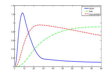
(b) Simulated concentration curves

Figure 1: Phantom of tested data and temporal concentration curves in all subregions.

The second numerical experiment is performed on a synthetic image simulating rat’s abdomen, where the bright region represents the heart of a rat. We use the TAC in Figure 2 to simulate the dynamic images.

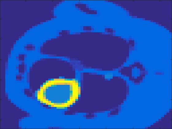
(a) Simulated image phantom

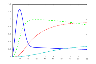
(b) Simulated concentration curves

Figure 2: Phantom of rat’s abdomen and temporal concentration curves in all subregions.

4.1 Gaussian noise

We compare our method with the filtered back projection (FBP) method, the results by alternatingly solving least square model $\arg\min_{\alpha,B}\|A\alpha B^{\top}-f\|_{F}^{2}$, our previous model, sparsity enforced matrix factorization(SEMF) proposed in [25]. As for the initial value of $U$, $\alpha$ and $B$, we use uniformed B-spline, $B\in\mathbb{R}^{90\times 20}$ as initial basis to solve $\arg\min_{\alpha,B}\|A\alpha B^{\top}-f\|_{F}^{2}$ for $\alpha$ and $B$. Then, the same $\alpha$, $B$, and $U=\alpha B^{T}$ are used as the initialization of $U$,$\alpha$ and $B$ to solve our proposed model.

In the tests, projections at two orthogonal angles are simulated for every frame to mimic 2-head camera data collection. The projection angles increase sequentially by $1^{\circ}$ along temporal direction. For example, at frame 1, projections are simulated at angle $1^{\circ}$ and $91^{\circ}$, and at frame 2, angle $2^{\circ}$ and $92^{\circ}$, etc. Finally, $10\%$ white Gaussian noise is added to the projection data. Reconstruction results with different methods are shown in Figure 3. Since the number of projections is very limited for each frame, the traditional FBP and least square methods cannot reconstruct the images satisfactorily, while the proposed method is capable to reconstruct the images effectively. Compared with SEMF model, when the edge of images jump (see frame 21 -frame 31 in Figure 3), the proposed model can better capture the change of the tendency of TAC.

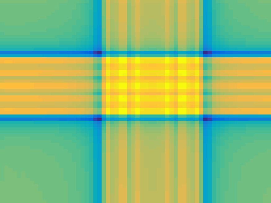
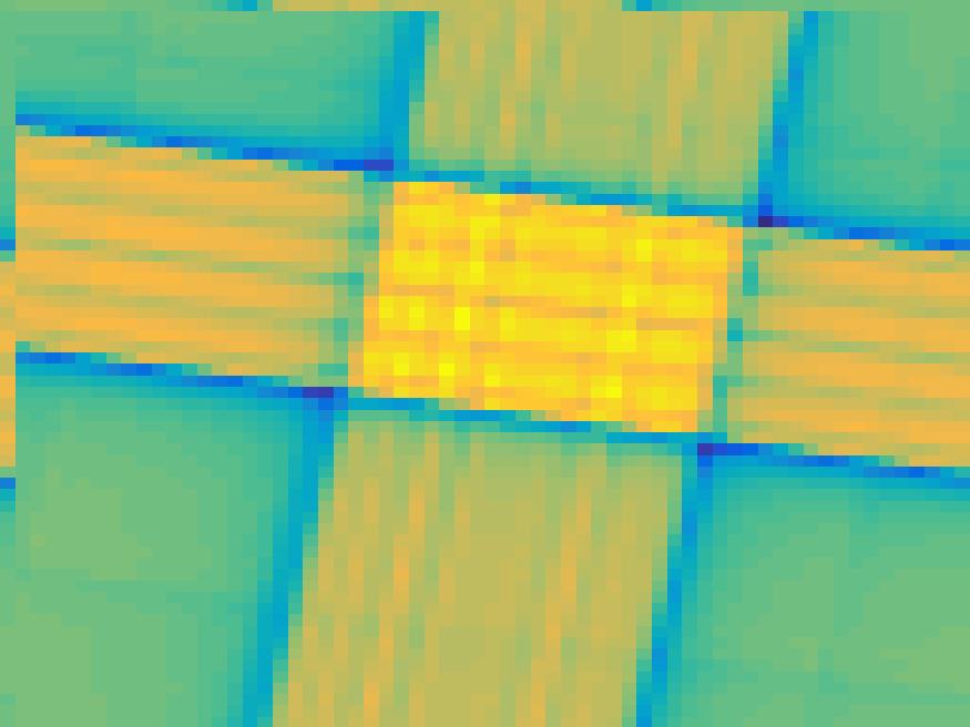
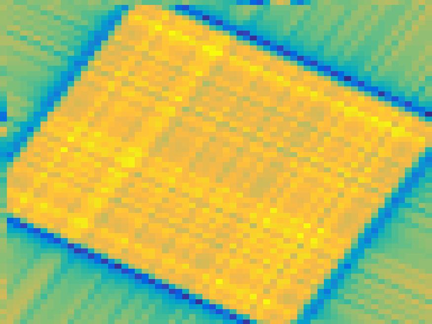
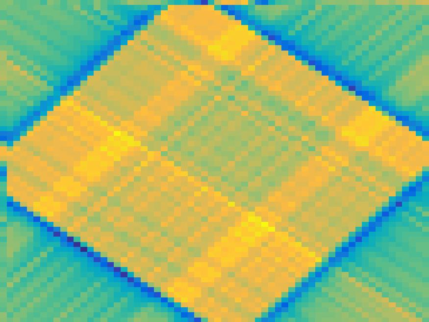
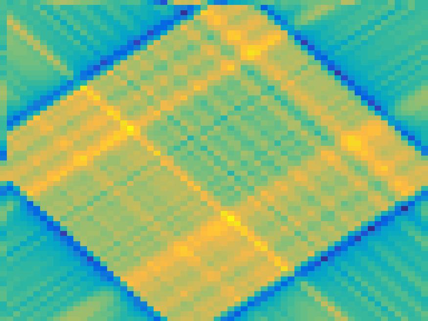
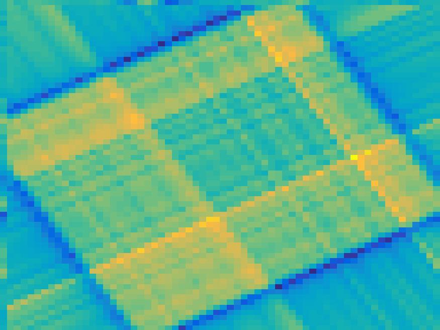
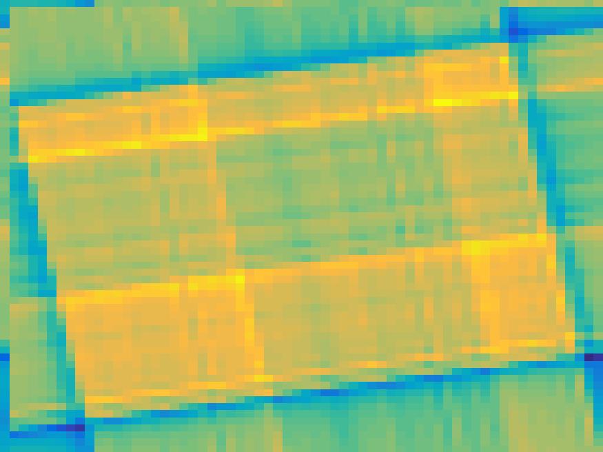
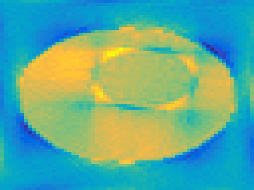
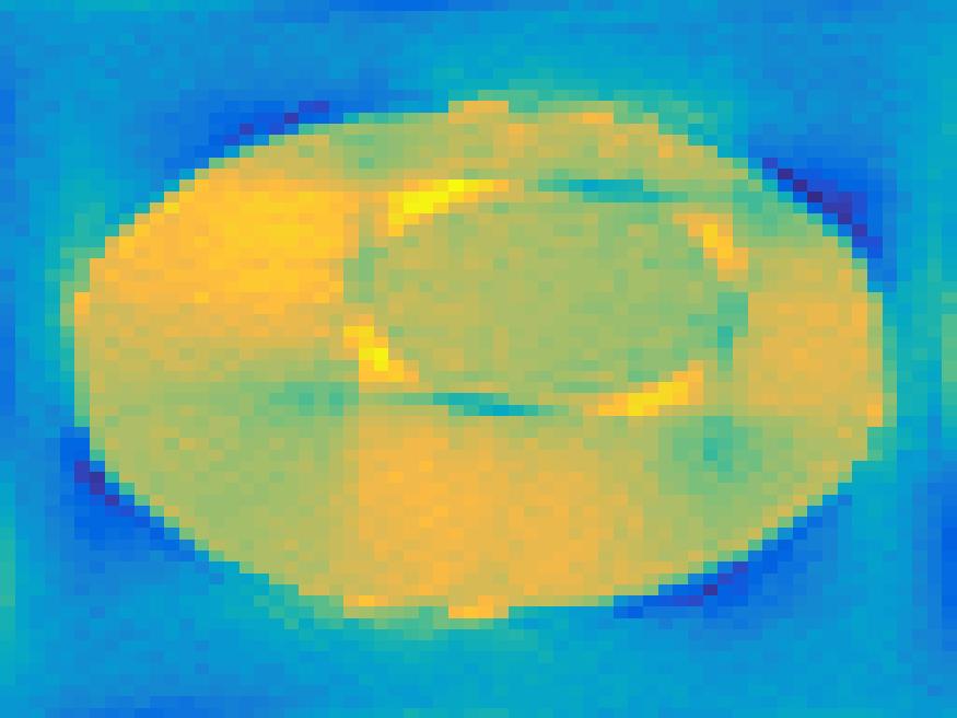
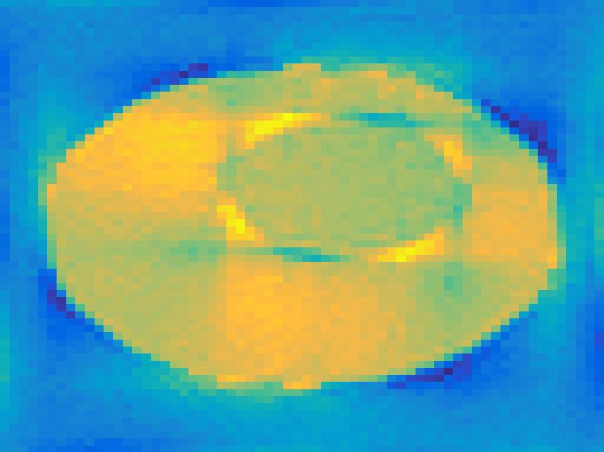
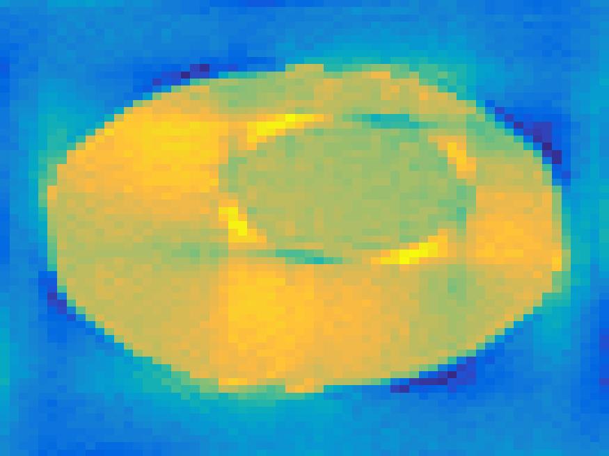
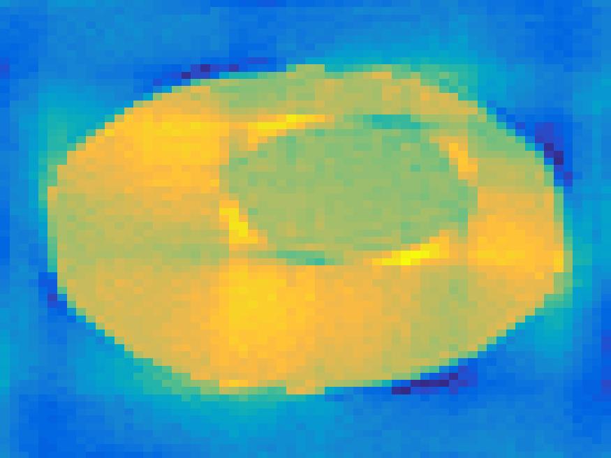
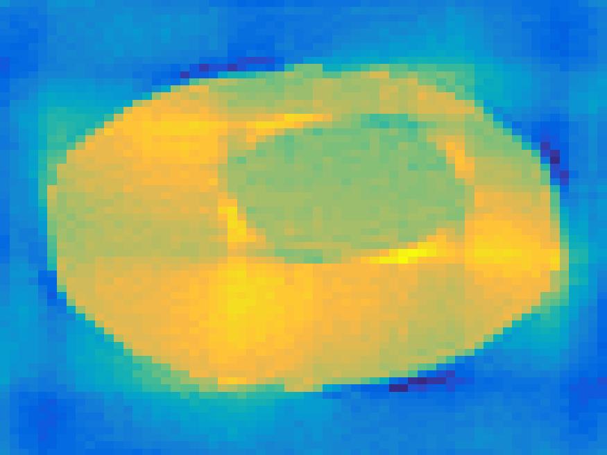
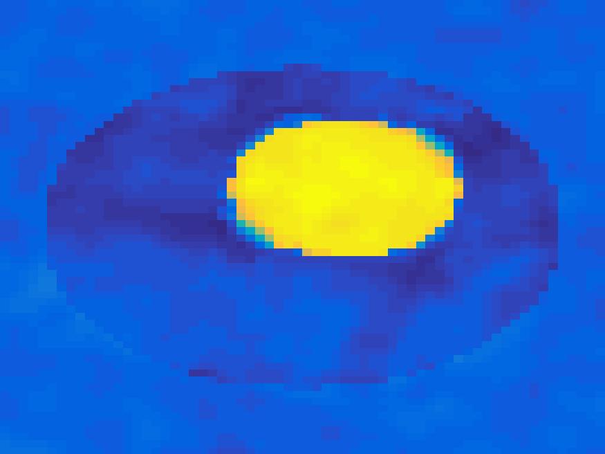
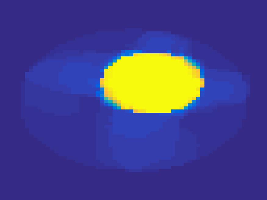
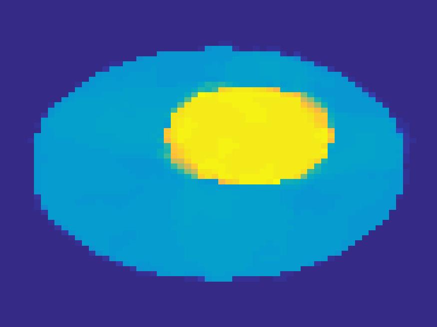
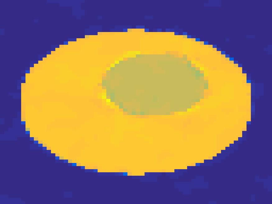
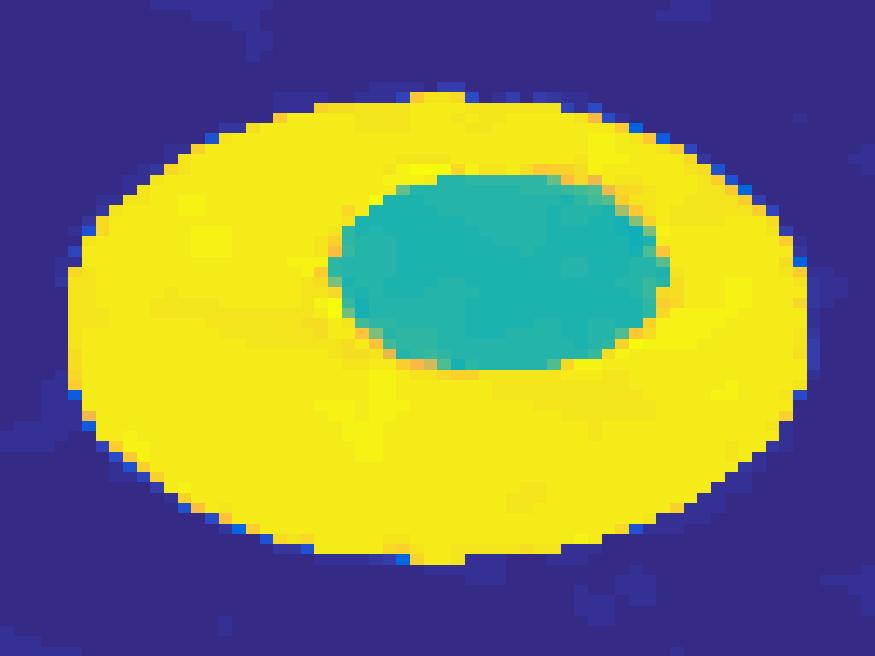
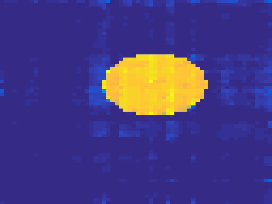
Frame 1	Frame 11	Frame 21	Frame 31	Frame 41	Frame 51	Frame 61	Frame 71	Frame 81

Figure 3: First row: Ground truth; Second row: FBP; Third row: least square method; Forth row: SEMF [25]; Fifth row: Proposed model.

Figure 4 illustrates the comparison of the TACs of blood and liver. The dash lines are the normalized true TACs and the solid lines are the normalized one extracted from the reconstruction images by our method. Even with high level noise and fast change of radioisotope, the reconstructed one fit closely to the true one.

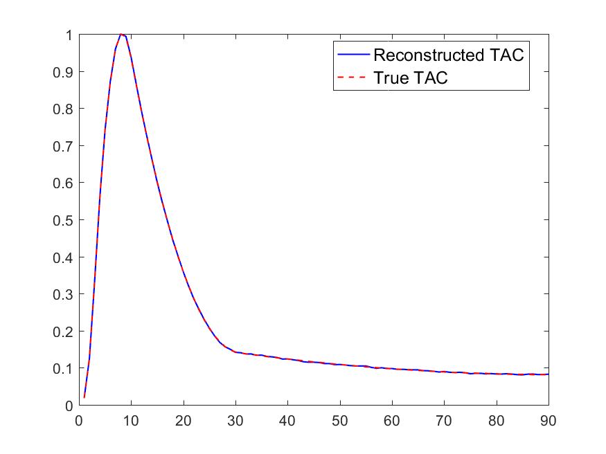
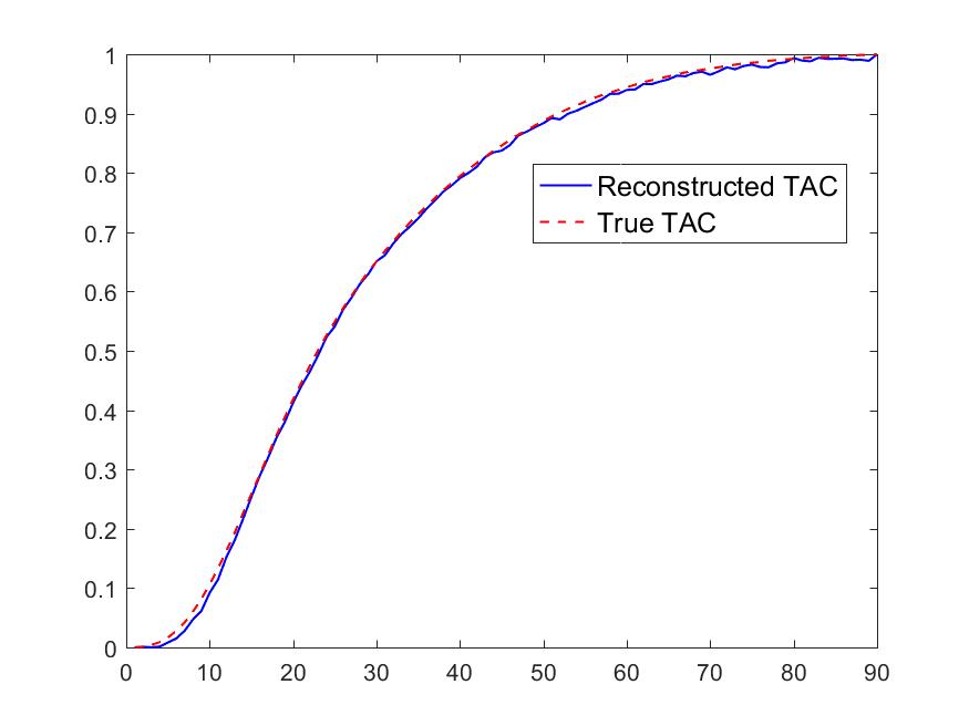
Figure 4: Time activity curve of two regions.

For the simulated images of rat’s abdomen, the same procedure is applied to generate projection data. Also, $10\%$ noise was added to the sinogram. Figure 5 compares the frames reconstructed by different methods. Clearly, the traditional FBP method and least square method cannot reconstruct the dynamic images with very few projections, however the proposed method reconstructs the images quite accurately. Figure 6 illustrates the comparison of the true TACs and those reconstructed by the proposed method. We can see that they are quite accurate and present small errors.

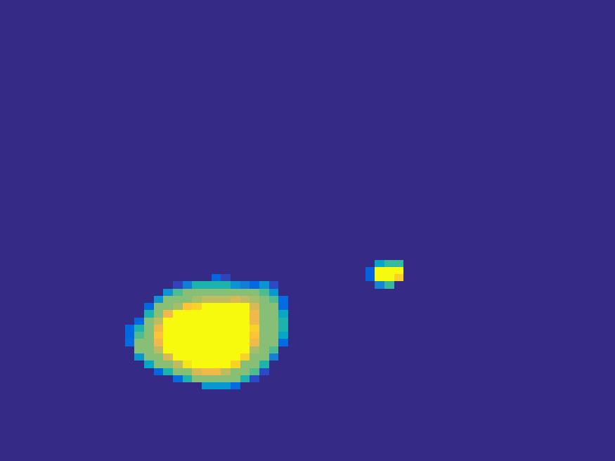
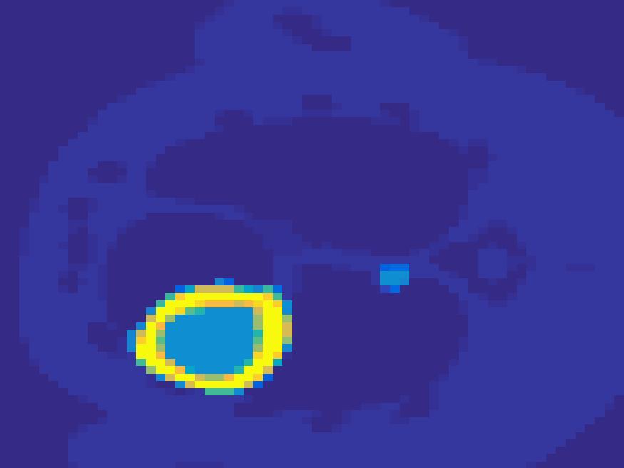
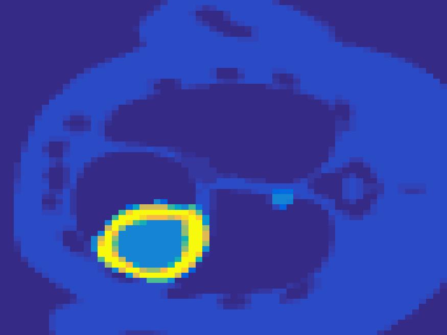
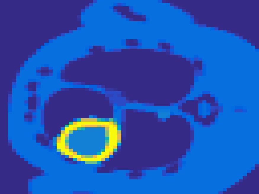
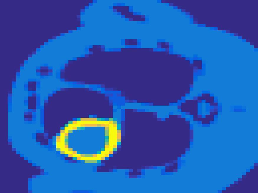
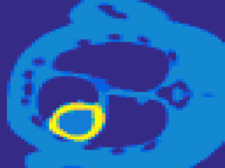
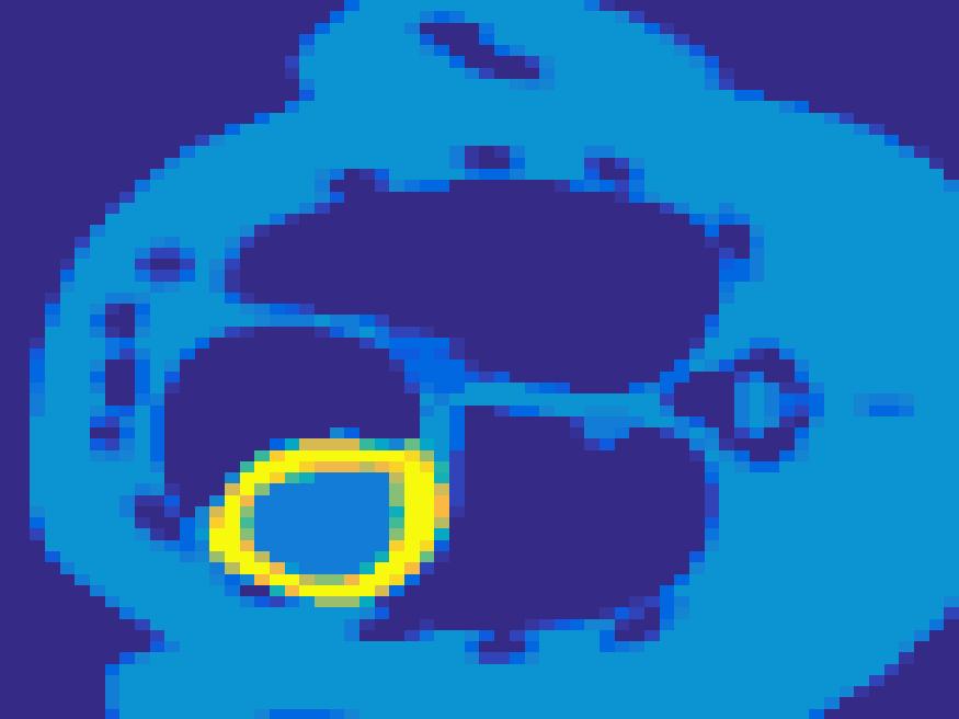
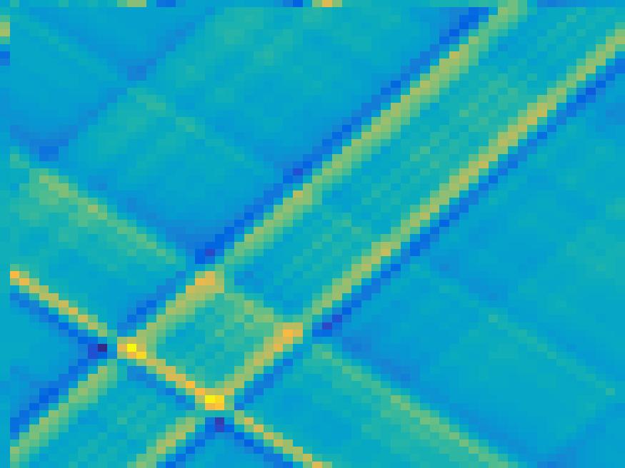
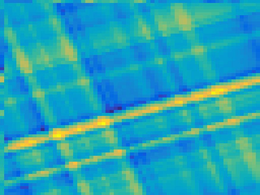
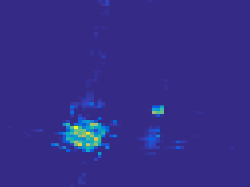
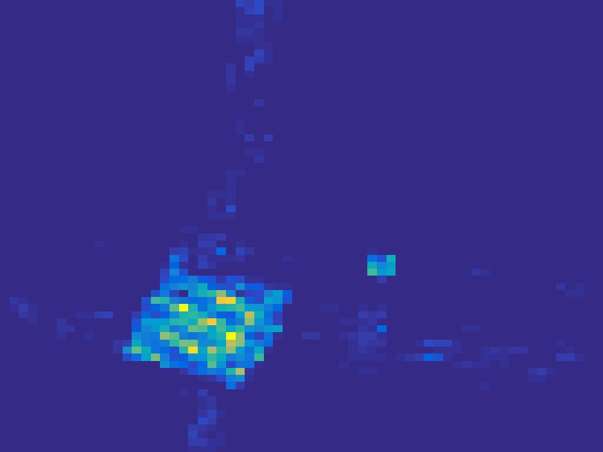
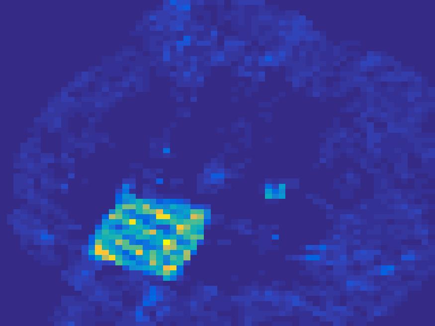
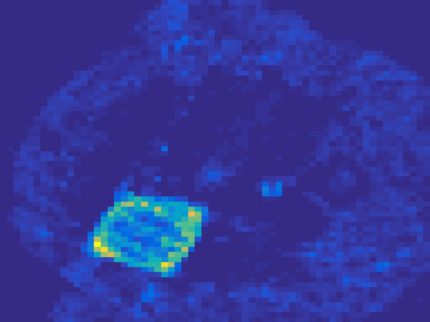
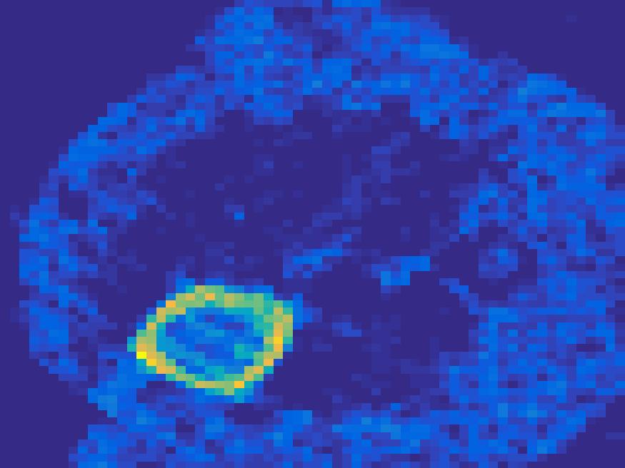
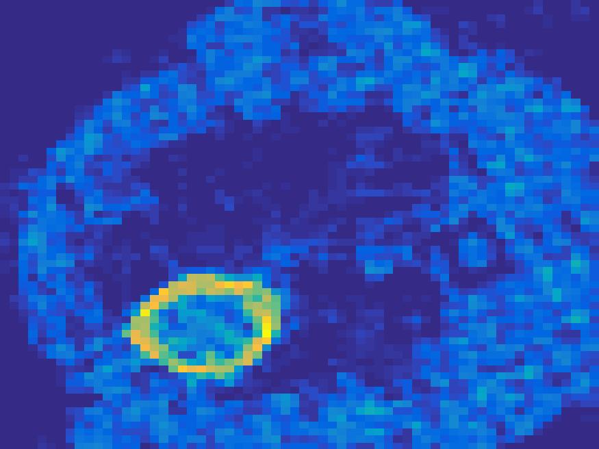
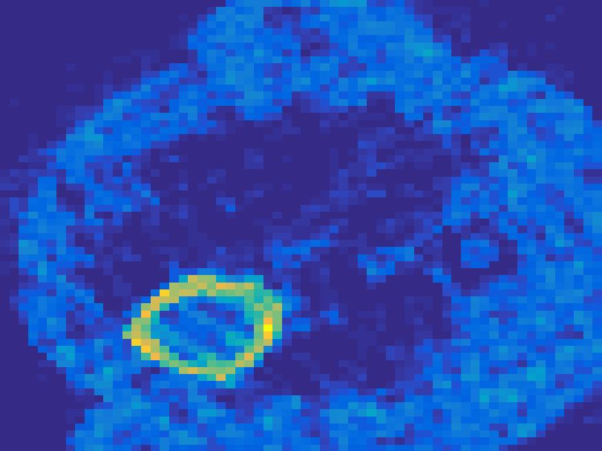
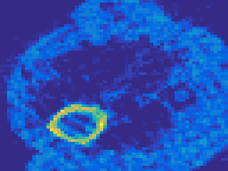
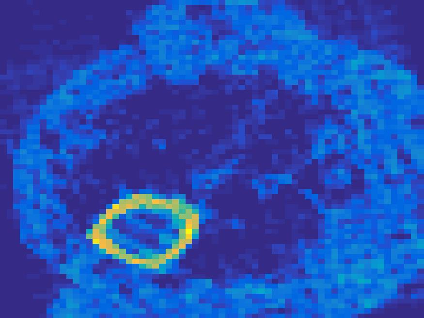
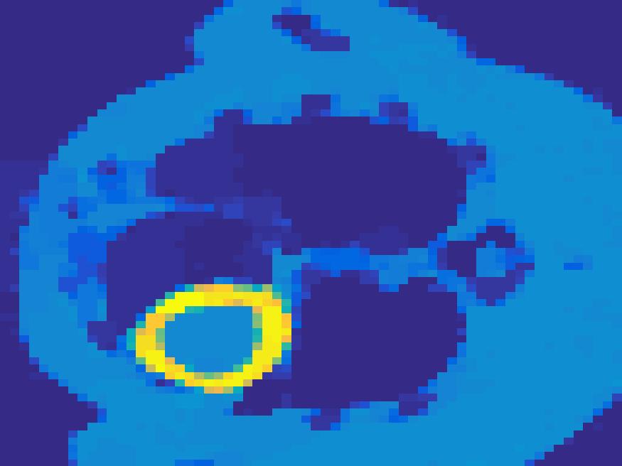
Frame 1	Frame 11	Frame 21	Frame 31	Frame 41	Frame 51	Frame 61	Frame 71	Frame 81

Figure 5: First row: Ground truth; Second row: FBP; Third row: least square method; Forth row: SEMF [25]; Fifth row: Proposed model.

Figure 6: Comparison of the true TACs and the reconstructed TACs by the proposed method.

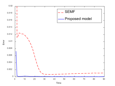
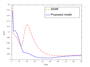
Figure 7: Comparison of the relative error for $t$-th frames by SEMF and the proposed method. Left: ellipse phantom; Right: rat’s abdomen phantom.

The relative error of the reconstructed image and the true one for $t$-th frame is defined as $\frac{\|U(:,t)_{rec}-U(:,t)_{true}\|_{2}^{2}}{\|U(:,t)_{true}\|_{2}^{2}}$, where $U_{rec}$ is the reconstructed frame by the proposed method and $U_{true}$ is the ground truth image. Figure 7 demonstrates the relative error of $T$ images reconstructed by proposed model and SEMF of two different datasets. The solid lines are the errors of the reconstruction images by proposed model and the dash lines are the errors of the reconstruction images by SEMF. We can see that the relative error is smaller by proposed model compared with SEMF. This is due to the fact that in the proposed method, we set the former and later images as reference and the referred images can provide edge information for the image.

4.2 Poisson noise

4.2.1 Simulated Poisson noise

In SPECT/PET, Poisson noise are usually more common. To obtain a Poisson corrupted projection data, we scale the data by the maximum of $f$ and corrupted the data with Poisson noise by using the Matlab command poissrnd. The reconstructed image is obtained by applying the proposed model on the rescaling back sinogram .

Again, the proposed method is compared with FBP, and alternating applying the EM algorithm and update of the basis for solving $\min_{\alpha,B}D_{KL}(f,A\alpha B^{T}).$ As for the initials $U$, $\alpha$ and $B$ of our methods, we use uniformed B-spline, $B\in\mathbb{R}^{90\times 20}$ as initial basis $B$ and solve the above model to obtain for $\alpha$ and $B$ and $U=\alpha B^{T}$.

Figure 8 and 9 show the results of the ellipse and rat phantom with Poisson noise. Since the number of projections is very limited and the corruption by Poisson noise, the reconstruction by both FBP and EM (with updating basis) are not satisfactory, while the proposed method is capable to reconstruct the main structure of the images faithfully.

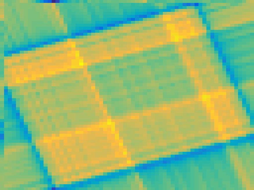
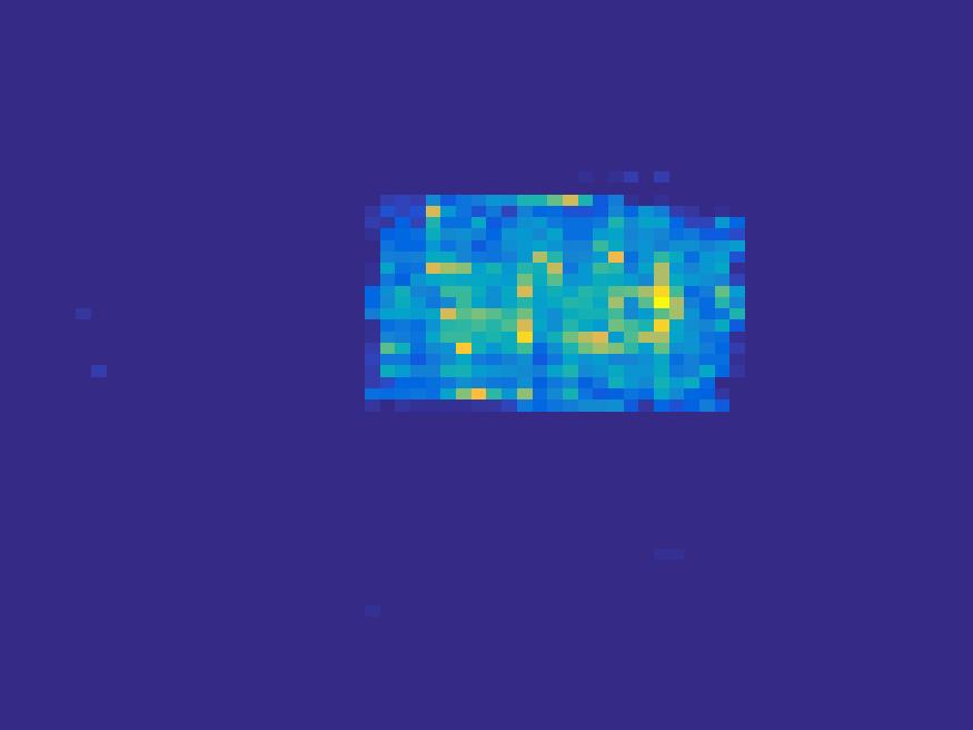
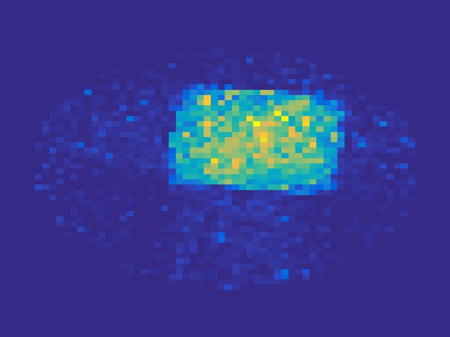
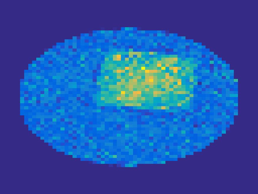
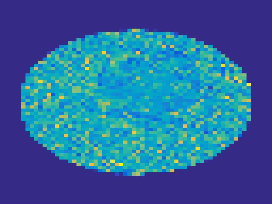
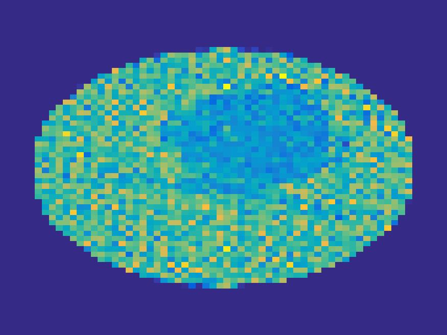
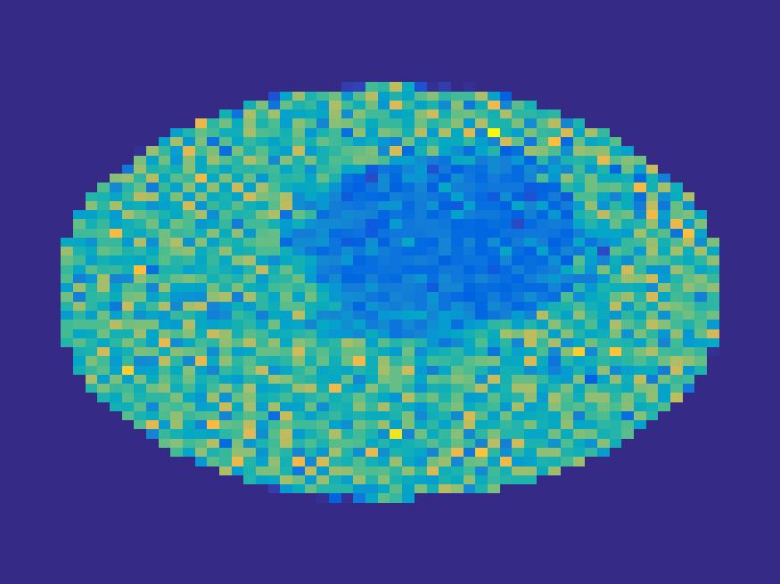
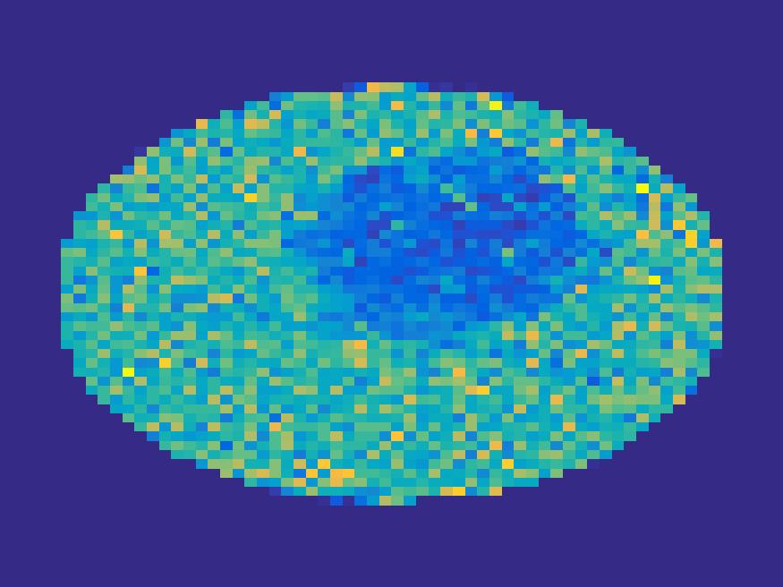
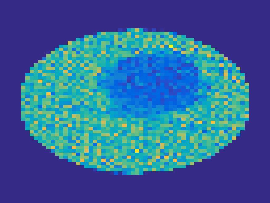
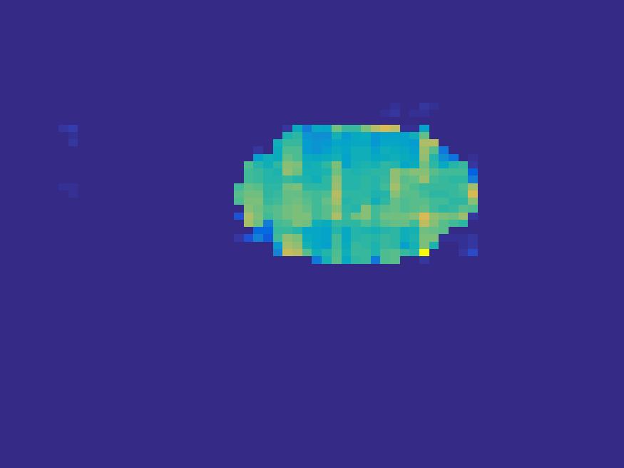
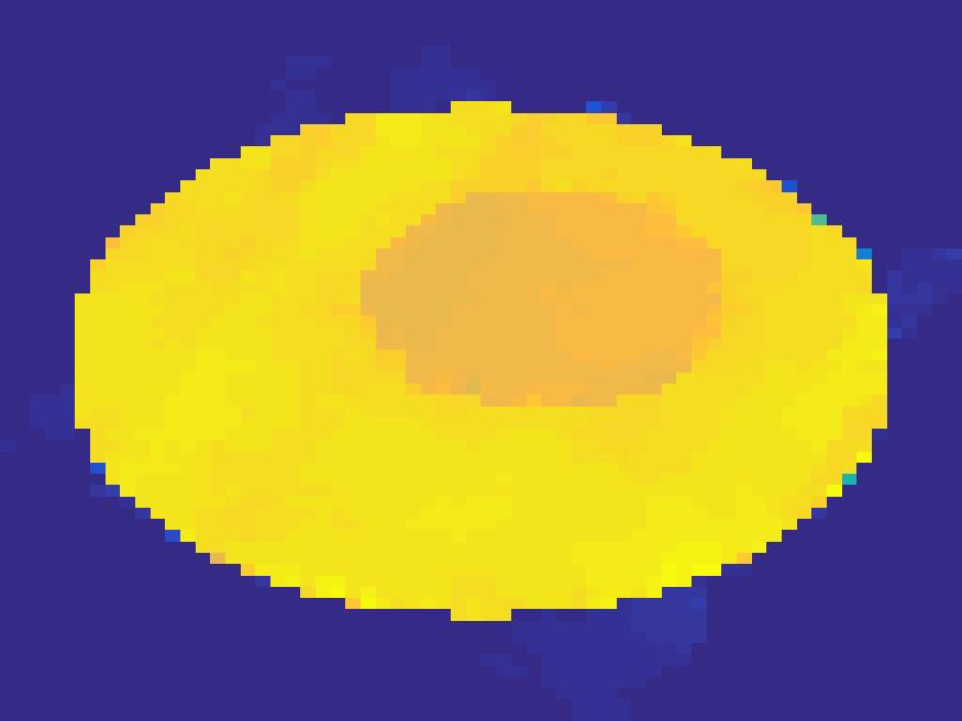
Frame 1	Frame 11	Frame 21	Frame 31	Frame 41	Frame 51	Frame 61	Frame 71	Frame 81

Figure 8: First row: Ground truth; Second row: FBP; Third row: EM algorithm with updating $\alpha$ and $B$; Forth row: Proposed method.

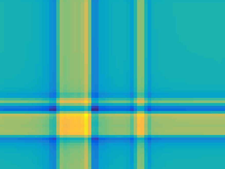
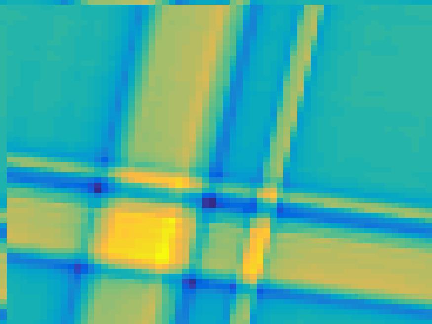
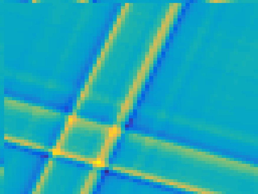
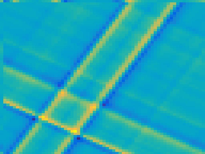
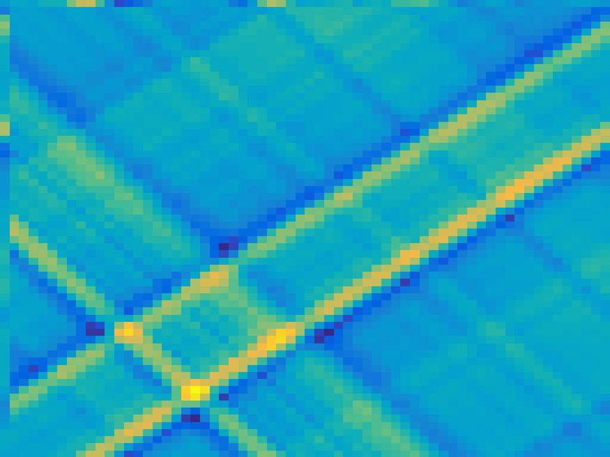
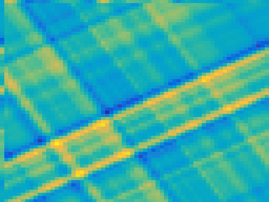
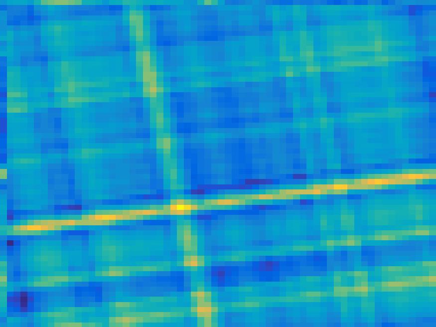
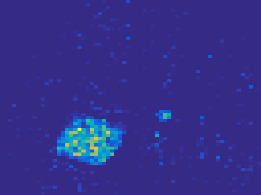
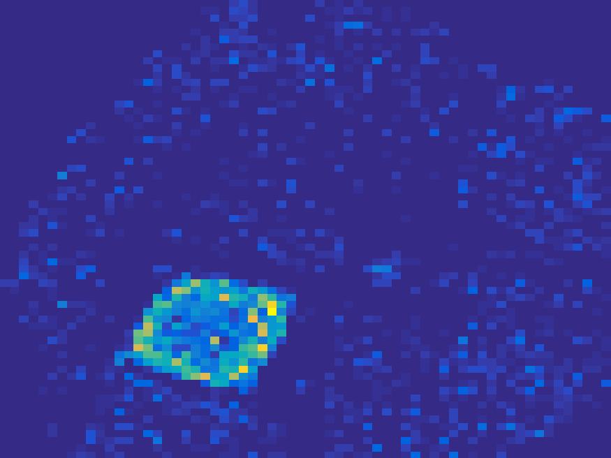
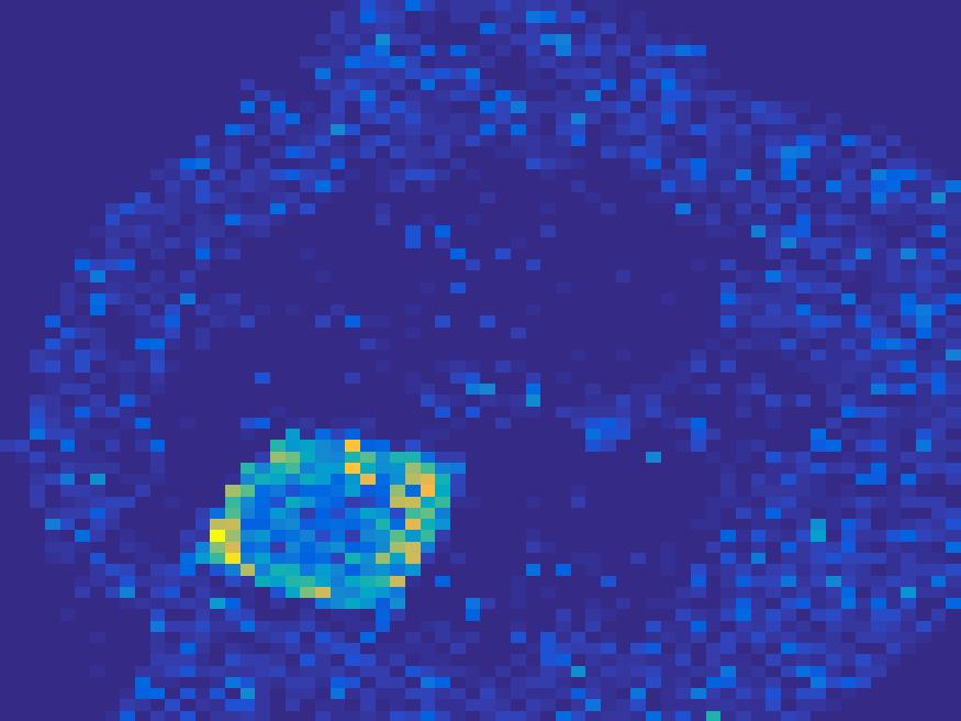
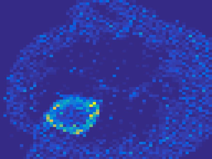
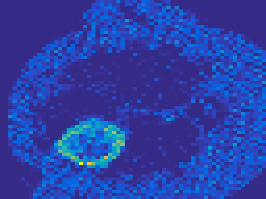
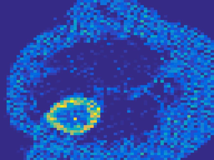
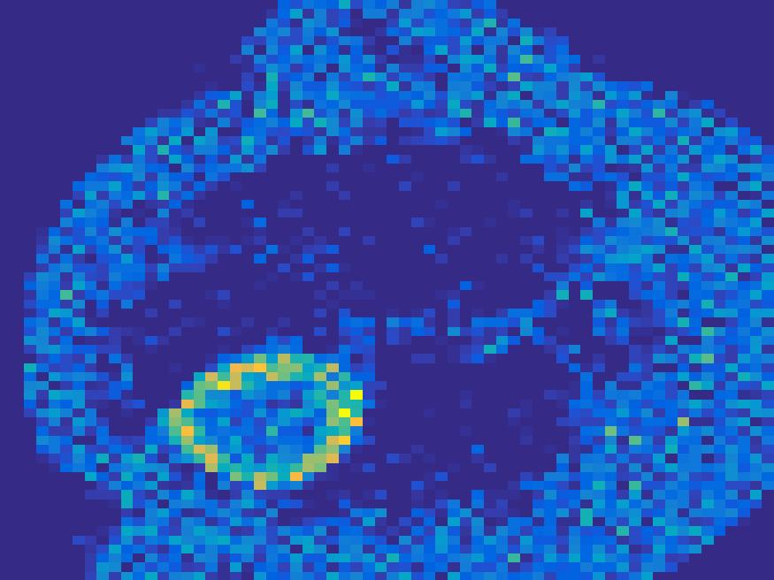
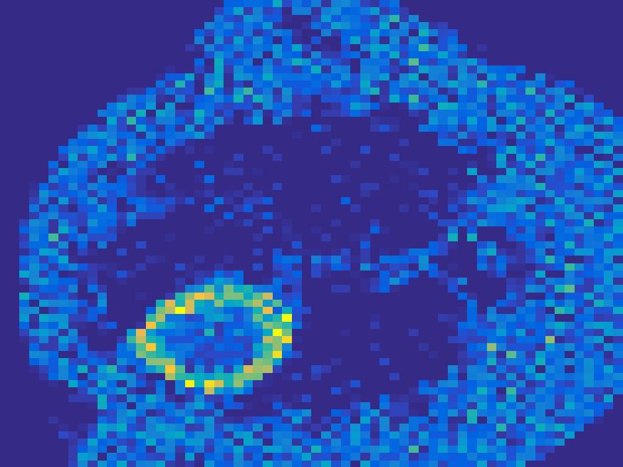
Frame 1	Frame 11	Frame 21	Frame 31	Frame 41	Frame 51	Frame 61	Frame 71	Frame 81

Figure 9: First row: Ground truth; Second row: FBP; Third row: EM algorithm with updating $\alpha$ and $B$; Forth row: Proposed method.

Figure 10 and 11 shows the comparison of the TACs of blood and liver for the two phantoms. The dash lines are the normalized true TACs and the solid lines are the normalized one extracted from the reconstruction images by our method. Even with high level noise and fast change of radioisotope, the reconstructed one fit closely to the true one.

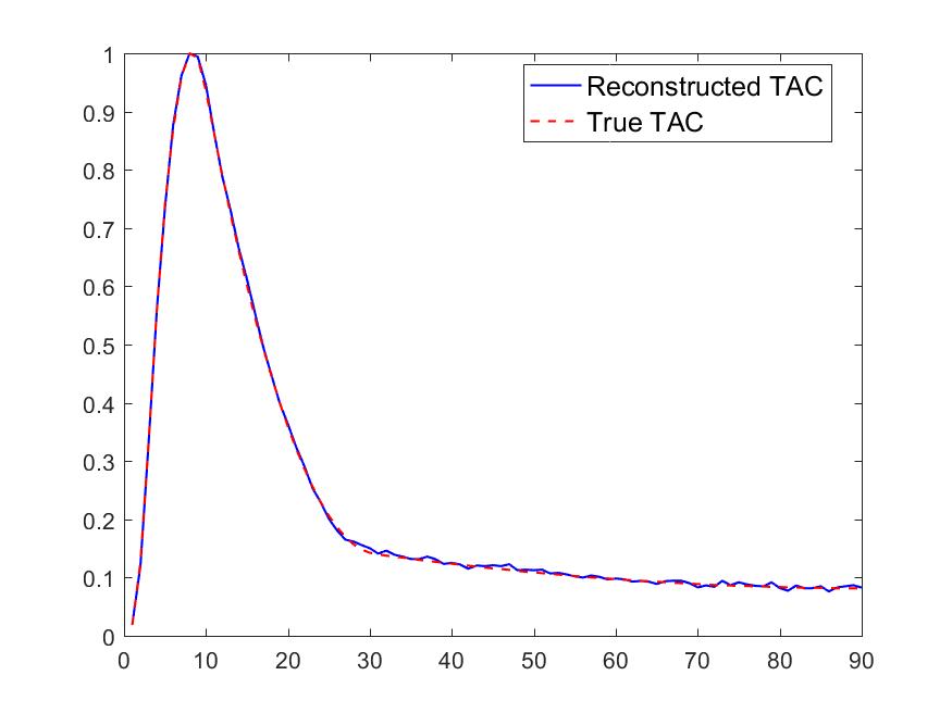
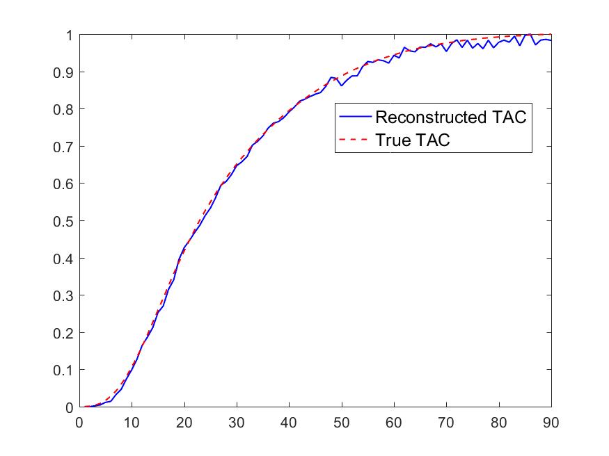
Figure 10: Comparison of the true TACs and the Reconstructed TACs in two regions (Ellipse phantom).

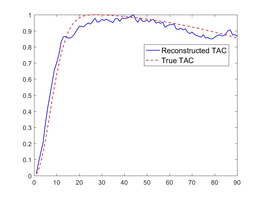
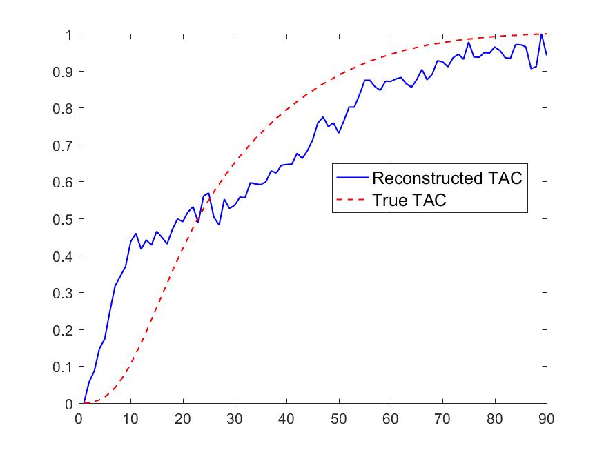
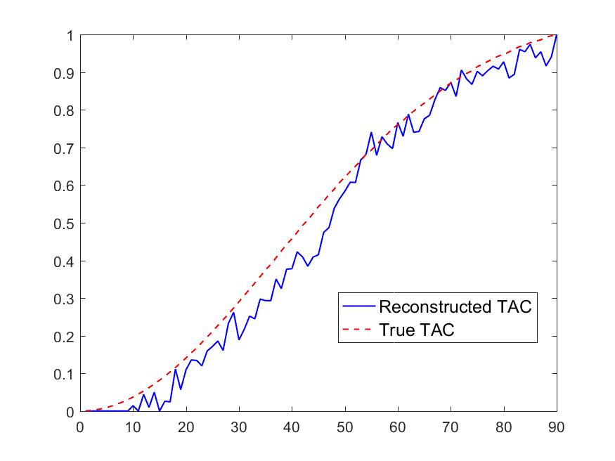
Figure 11: Comparison of true TACs and Reconstructed TACs in four regions (Rat’s abdomen phantom).

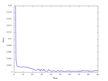
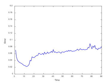
Figure 12: The relative error of the image reconstructed by proposed method with poisson noisy data. The left is error of the first numerical experiment and the right is the second one.

Figure 12 demonstrates the relative error of the image reconstructed by the proposed method with poisson noisy data for the two dataset. By the proposed model, the relative error are small for the proposed method, while for the structure of the second image is complex, the relative error is bigger than the first one.

4.2.2 Monte Carlo simulation

In order to test the performance of the proposed method in a more realistic scenario, we perform a Monte Carlo simulation for dynamic SPECT imaging. First, we created a $129\times 129$ phantom image consisting of three circles as region of interests, shown in Figure 13. The TAC over a time period of 90 time steps of the outer and the two inner circles were displayed in 13(b).

For each single frame, the photon counts is a probability proportional to the concentration in every region. The events are detected by a virtual double heads gamma camera rotating around the patient by $1$ degrees per time step, which consists of $374$ detector bins. Every simulated decay event is projected and counted by the corresponding detector bin.

(a) Simulated image Phantom

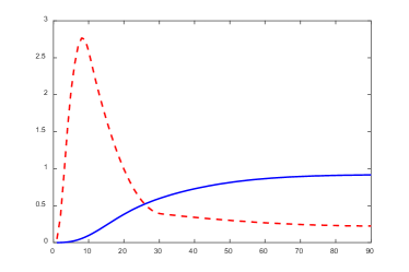
(b) Simulated concentration curves

Figure 13: Monte Carlo simulation. Blue solid line corresponds to the outer circle, red dash line corresponds to the two inner circles.

We set the number of events counted by the detector as $\mathrm{events}=2\times 10^{4}$ and $\mathrm{events}=2\times 10^{5}$) times the average concentration in one pixel of two different tests. The signogram images the count in each bin of two settings are shown in Figure 14.

(a) sinogram for $\mathrm{events}=20000$

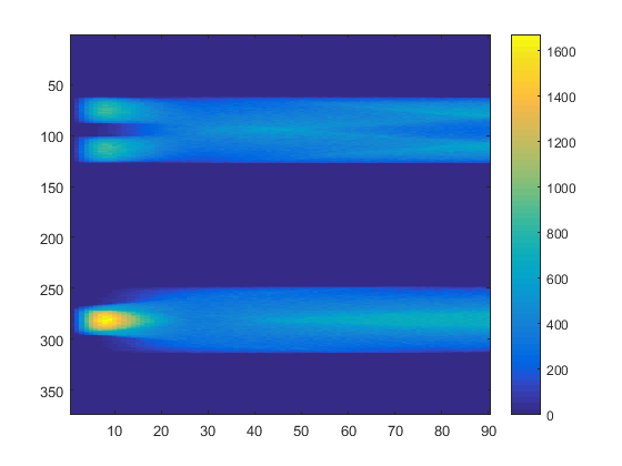
(b) sinogram for $\mathrm{events}=200000$

Figure 14: Monte Carlo sinogram data.

Based on the sinogram data, we compare the proposed method with the alternating EM algorithm. The results for both test cases are shown in Figure 15. We can see that for the case of a low count number, the proposed method is able to reconstruct the regions properly. Within a number of iterations, the algorithm presents a reasonable reconstruction of the region of interest and the corresponding regional tracer concentration curves.

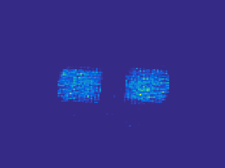
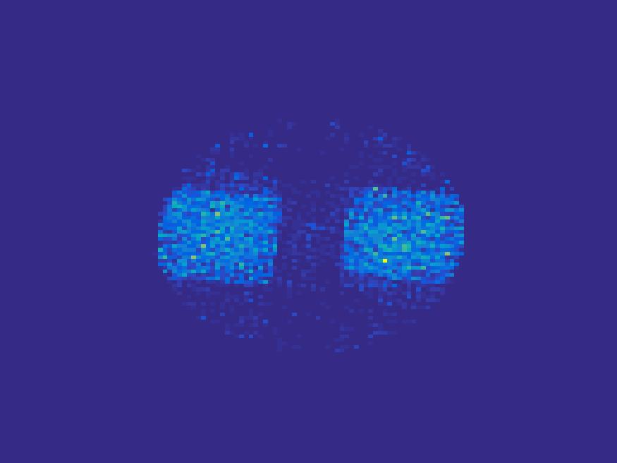
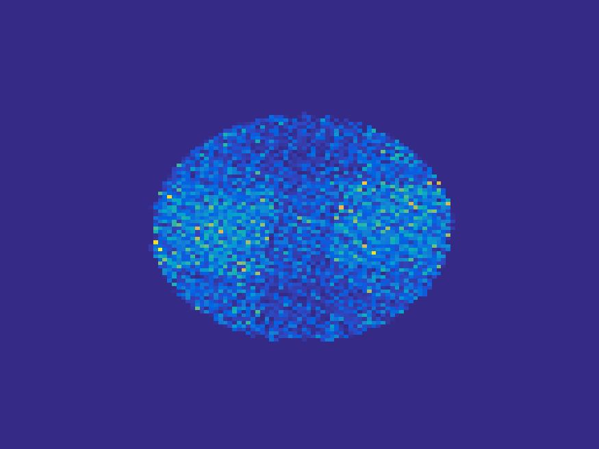
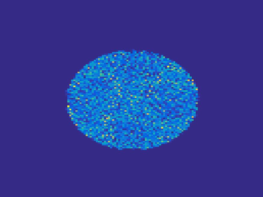
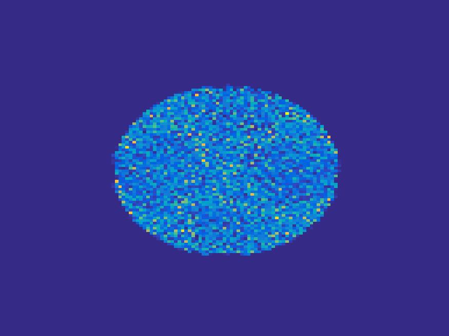
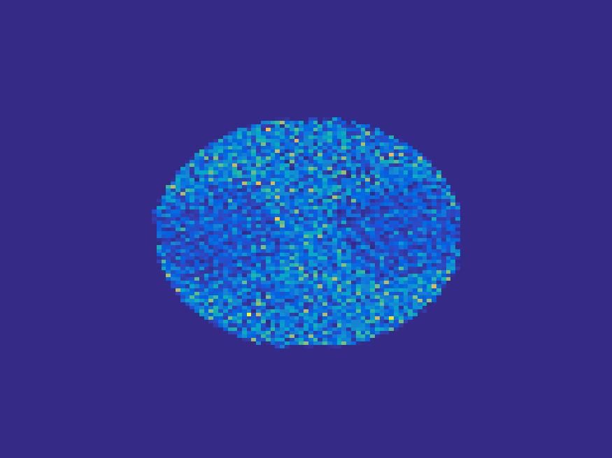
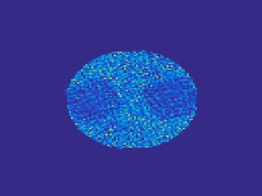
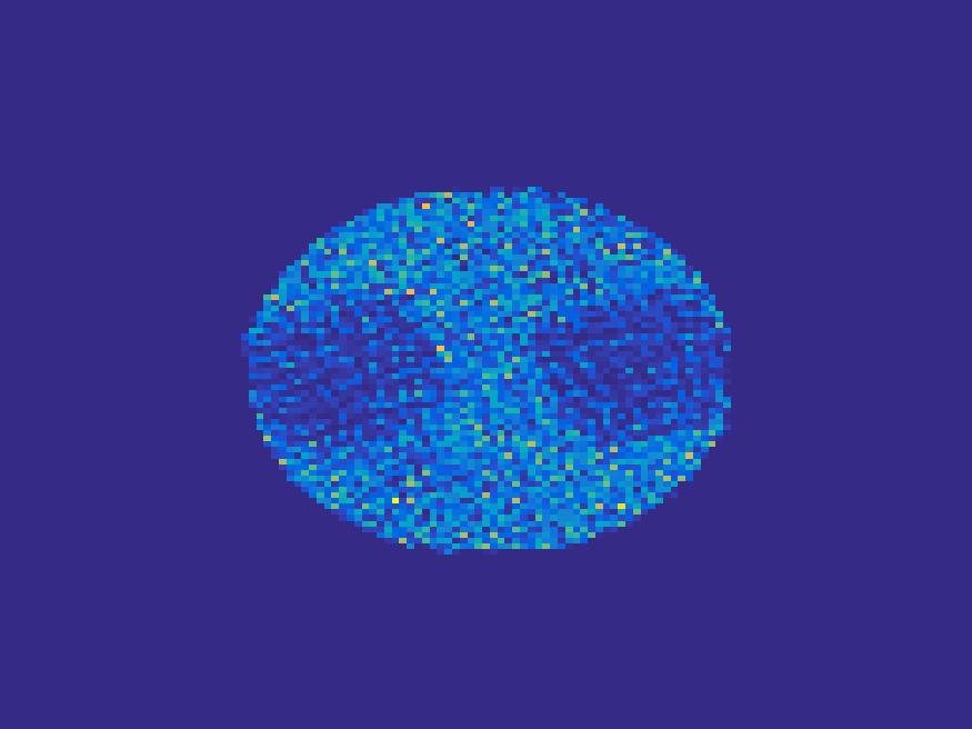
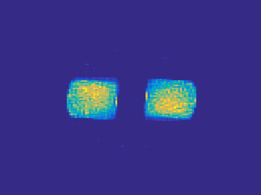
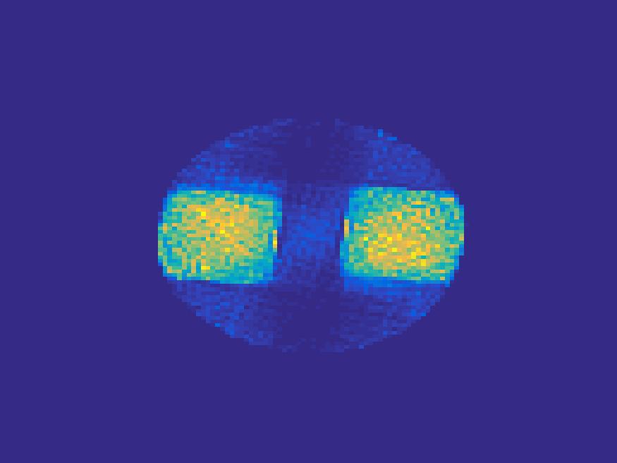
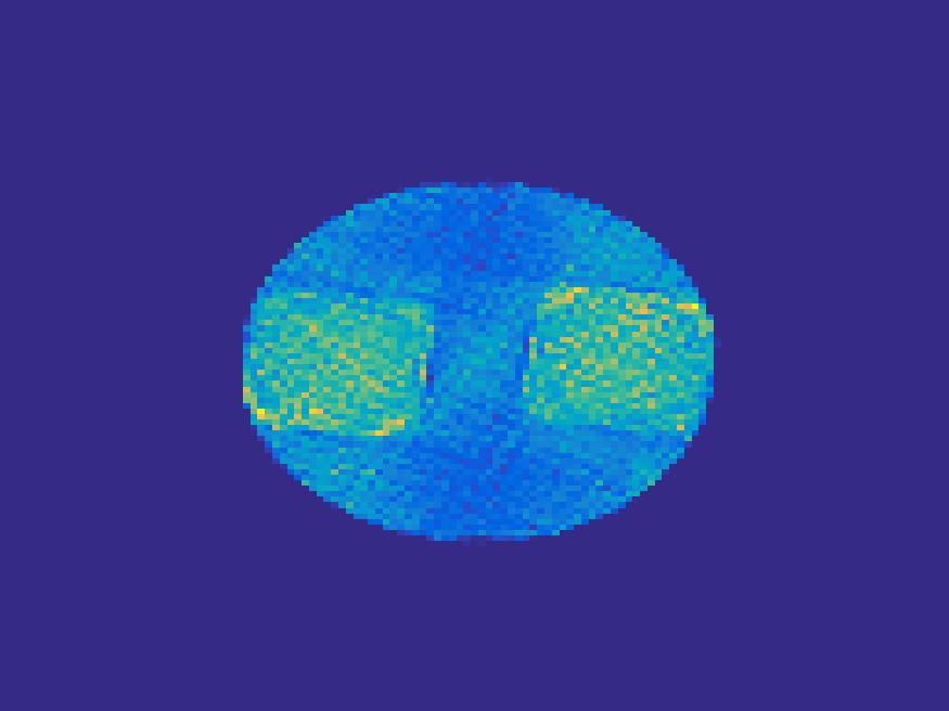
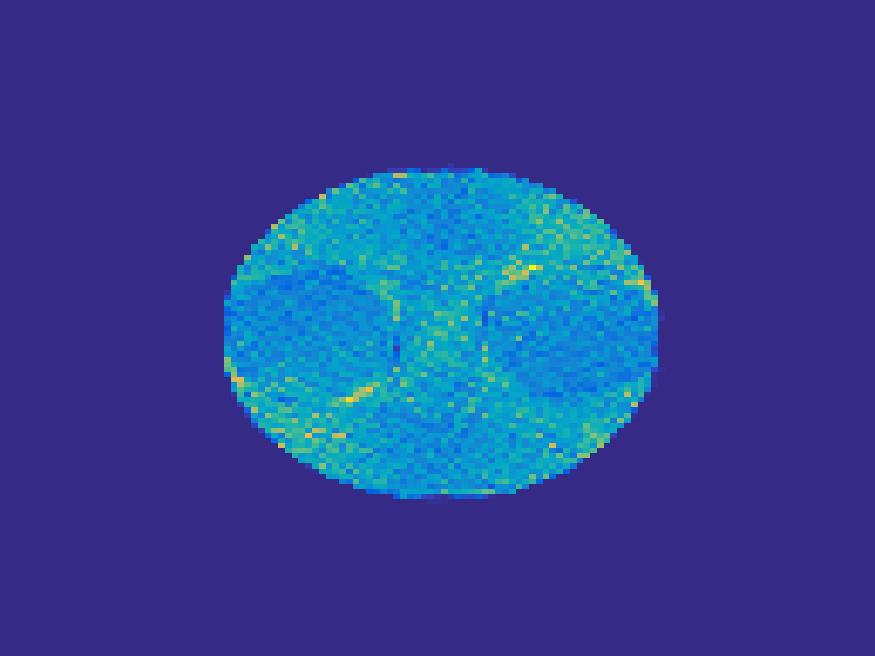
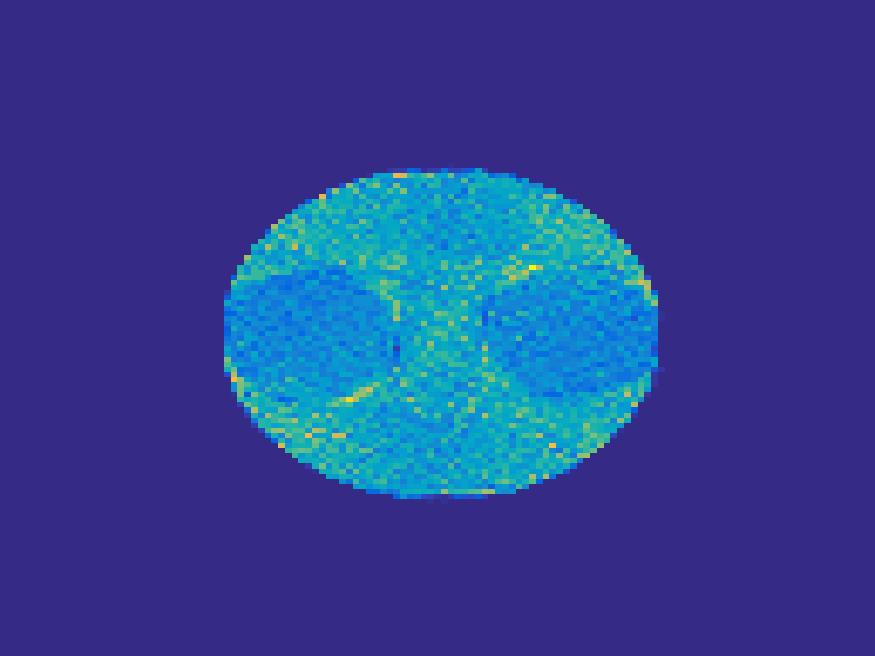
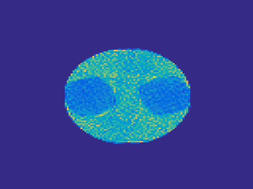
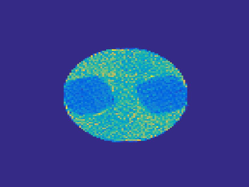
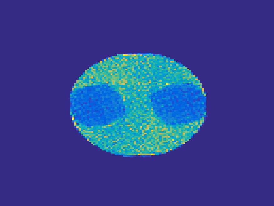
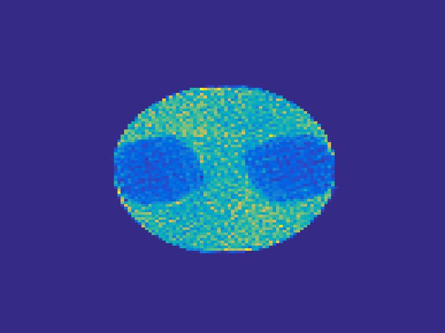
Frame 1	Frame 11	Frame 21	Frame 31	Frame 41	Frame 51	Frame 61	Frame 71	Frame 81

Figure 15: Reconstruction with Monte Carlo simulated data. First row: Ground truth. Second and third row are the results with $\mathrm{events}=20000$. Second row : EM with updating $\alpha$ and $B$; third row: proposed method. Forth and fifth row are the results with $\mathrm{events}=200000$. Forth row: EM with updating $\alpha$ and $B$; Fifth row: proposed method.

Figure 16 illustrates the comparison of the TACs of two regions. The dash lines are the normalized true TACs and the solid lines are the normalized one extracted from the reconstruction images by our method. The first row are TACs of the events equal to $20000$ and the second row are TACs of $200000$ events.

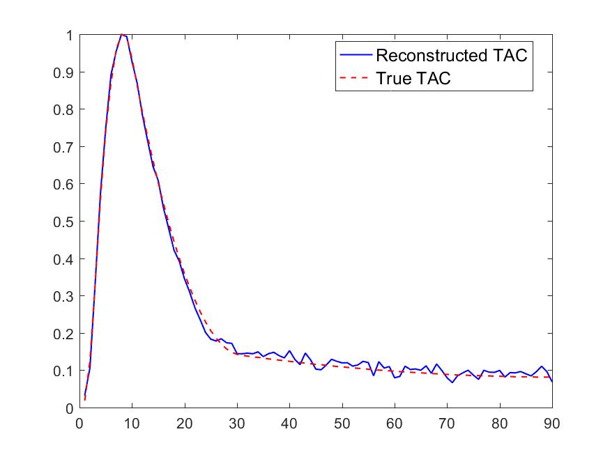
(a) TAC of $\mathrm{events}=20000$

(b) TAC of $\mathrm{events}=20000$

(c) TAC of $\mathrm{events}=200000$

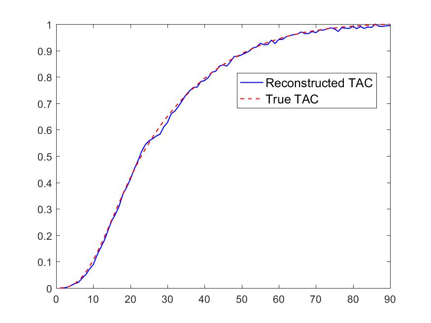
(d) TAC of $\mathrm{events}=200000$

Figure 16: Time activity curve of two regions.

We also perform Monte carlo simulation on the more complex images: the rat’s abdomen phantom. By setting $\mathrm{events}=200000$, the sinogram image is shown in Figure 17.

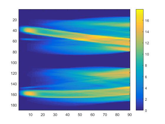
(a) Noiseless sinogram

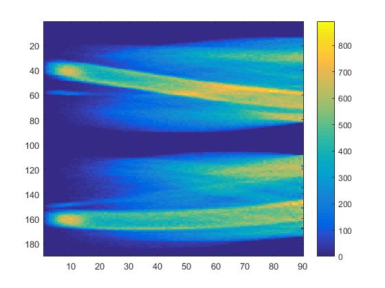
(b) sinogram for $\mathrm{events}=200000$

Figure 17: Monte Carlo sinogram data.

The images reconstructed can be found in Figure 18 for $\mathrm{events}=200000$. Figure 19 illustrates the comparison of the true TACs and those reconstructed by the proposed method. We can see that the proposed method is robust to reconstruct most of the structures present in the images.

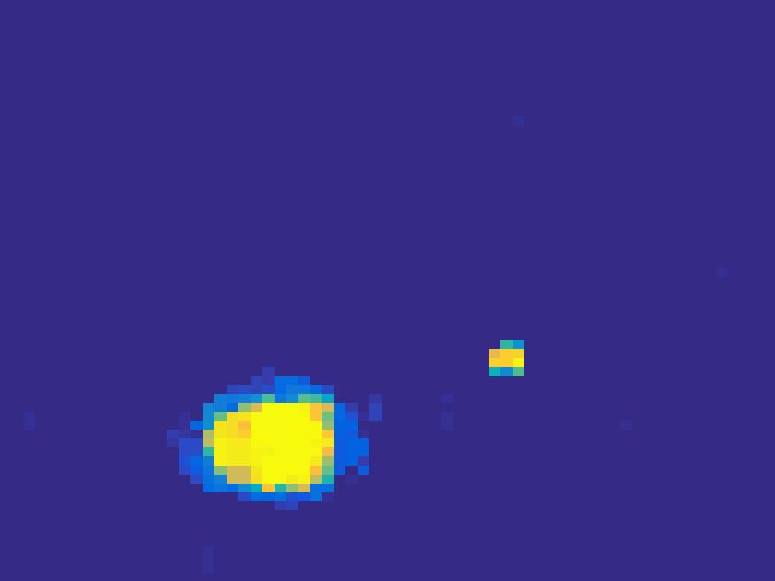
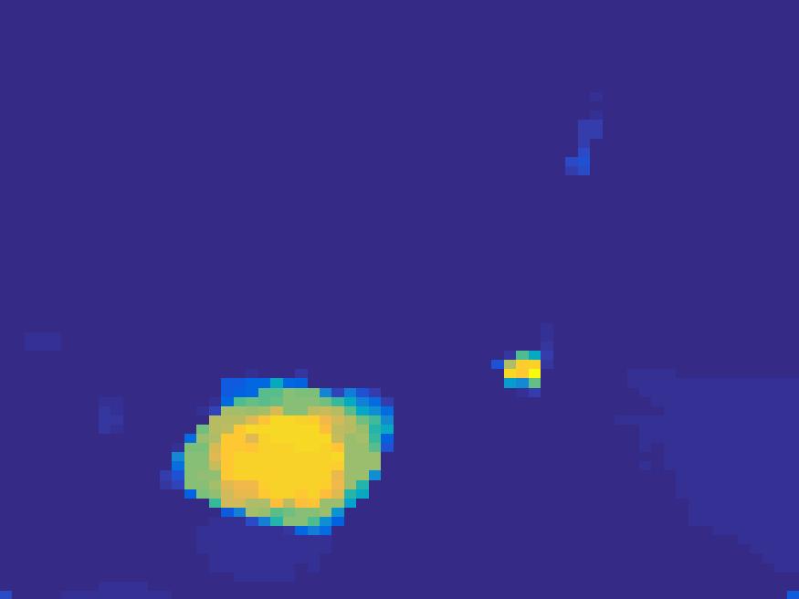
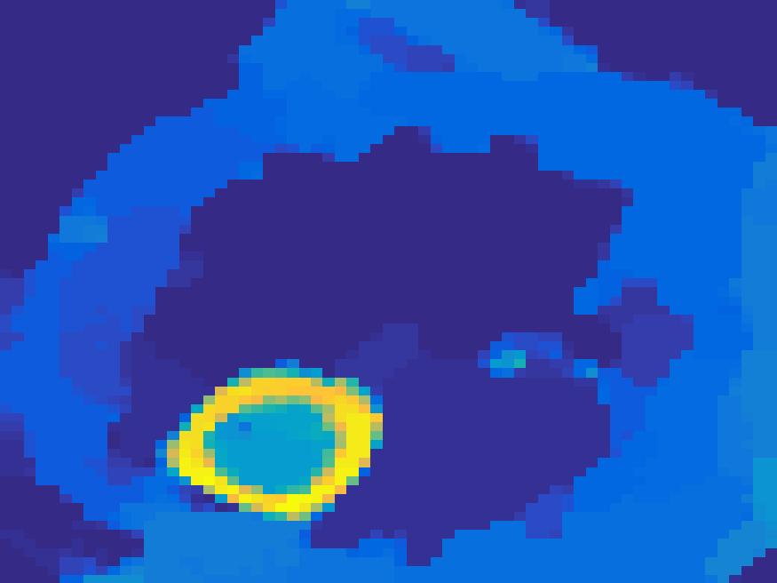
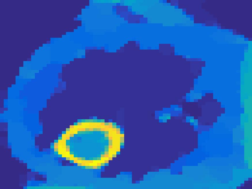
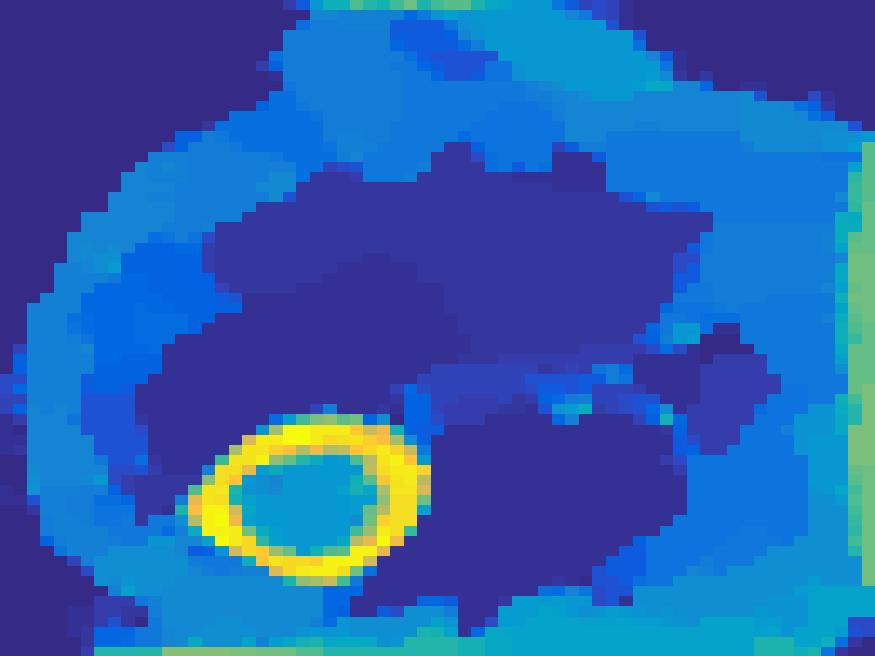
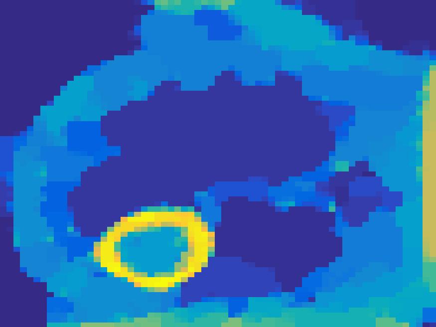
Frame 1	Frame 11	Frame 21	Frame 31	Frame 41	Frame 51	Frame 61	Frame 71	Frame 81

Figure 18: Reconstruction of Monte Carlo simulated data. First row: Ground truth; Second row : $\mathrm{events}=200000$, EM with updating $\alpha$ and $B$; third row: proposed method.

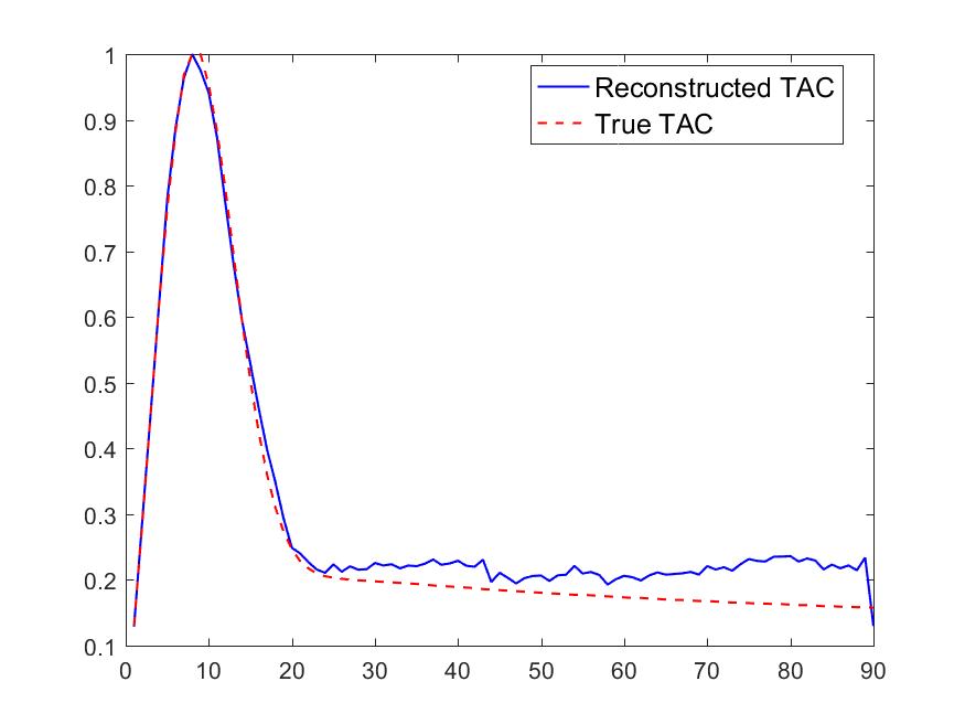
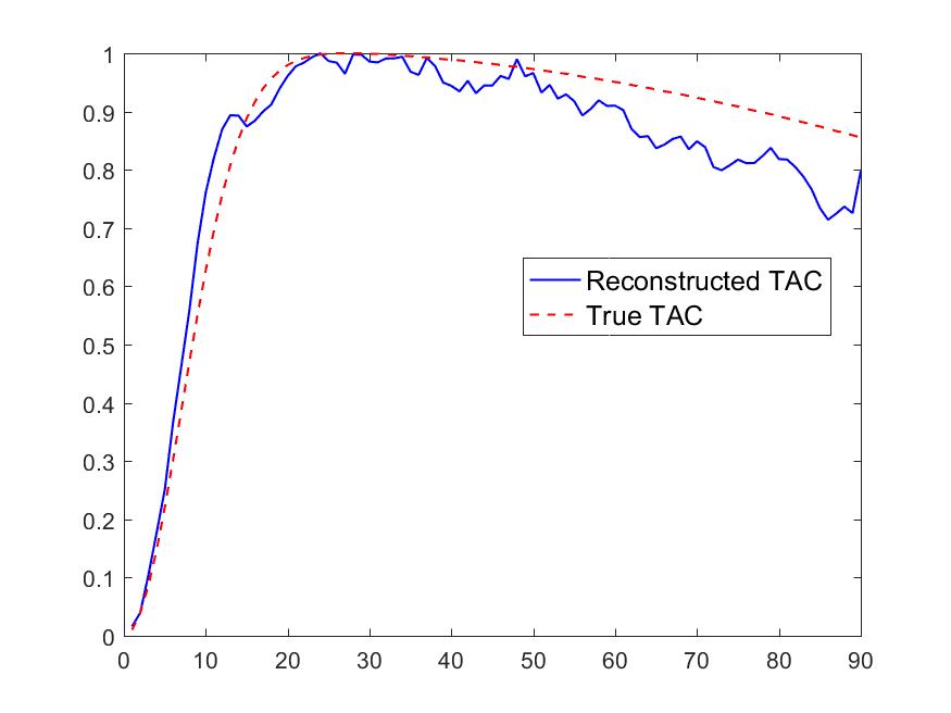
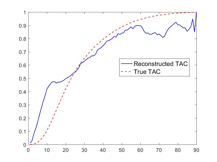
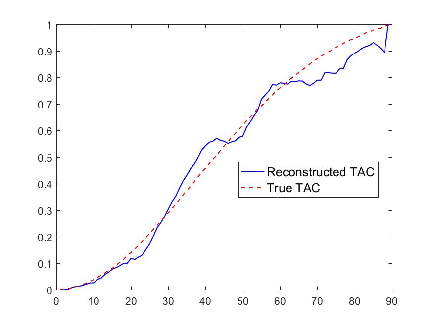
Figure 19: Reconstructed TACs.

5 Conclusion and Outlook

In this paper, we presented a new reconstruction model for dynamic SPECT from few and incomplete projections based on edge correlation. Both Gaussian noise and Poisson noise are investigated. The proposed nonconvex model is solved by an alternating scheme. The reconstruction results on two 2D phantoms indicate that our algorithm outperforms the conventional FBP type reconstruction algorithm, least square/EM method and the former SEMF model. The reconstructed image sequences are very close to the exact ones, especially for those frames with changed edge directions. Extensive numerical results show that the choice of the regularization methods as well as the reconstruction approach is effective for a proof of concept study. Nevertheless, there are still many aspects that needs to be improved in future. Firstly, the method is tested on simulated 2D images with low spatial resolution while real clinical dynamic SPECT is 3D with higher spatial resolution. Consequently, computation time and acceleration method should be taken the into account. Furthermore, the model involves many parameters that needs to be set in a more automatical way. Therefore it is necessary to discuss the parameter choice in a future work.

References

References

- [1] Yehuda Vardi, LA Shepp, and Linda Kaufman. A statistical model for positron emission tomography. Journal of the American Statistical Association, 80(389):8–20, 1985.
- [2] Joonyoung Kim, Pilar Herrero, Terry Sharp, Richard Laforest, Douglas J Rowland, Yuan-Chuan Tai, Jason S Lewis, and Michael J Welch. Minimally invasive method of determining blood input function from PET images in rodents. Journal of Nuclear Medicine, 47(2):330–336, 2006.
- [3] Gregory Z Ferl, Xiaoli Zhang, Hsiao-Ming Wu, and Sung-Cheng Huang. Estimation of the 18F-FDG input function in mice by use of dynamic small-animal PET and minimal blood sample data. Journal of Nuclear Medicine, 48(12):2037–2045, 2007.
- [4] Kooresh I Shoghi and Michael J Welch. Hybrid image and blood sampling input function for quantification of small animal dynamic PET data. Nuclear medicine and biology, 34(8):989–994, 2007.
- [5] Grant T Gullberg, Bryan W Reutter, Arkadiusz Sitek, Jonathan S Maltz, and Thomas F Budinger. Dynamic single photon emission computed tomography basic principles and cardiac applications. Physics in medicine and biology, 55(20):R111, 2010.
- [6] Andrew J Reader and Jeroen Verhaeghe. 4D image reconstruction for emission tomography. Physics in Medicine and Biology, 59(22), 2014.
- [7] Eleonora Vanzi, Andreas Robert Formiconi, Dino Bindi, Giuseppe La Cava, and Alberto Pupi. Kinetic parameter estimation from renal measurements with a three-headed SPECT system: A simulation study. Medical Imaging, IEEE Transactions on, 23(3):363–373, 2004.
- [8] Hideki Sugihara, Yoshiharu Yonekura, Ken Kataoka, Daisuke Fukai, Nobuyasu Kitamura, and Yoshimitsu Taniguchi. Estimation of coronary flow reserve with the use of dynamic planar and SPECT images of Tc-99m tetrofosmin. Journal of Nuclear Cardiology, 8(5):575–579, 2001.
- [9] Robert C. Marshall, Patricia Powersrisius, Bryan W Reutter, Scott E Taylor, Henry F Vanbrocklin, Ronald H Huesman, and Thomas F. Budinger. Kinetic Analysis of 125I-Iodorotenone as a Deposited Myocardial Flow Tracer: Comparison with 99mTc-Sestamibi. The Journal of Nuclear Medicine, 42(2):272–281, 2001.
- [10] Richard E Carson. A maximum likelihood method for region-of-interest evaluation in emission tomography. Journal of computer assisted tomography, 10(4):654–663, 1986.
- [11] Andreas Robert Formiconi. Least squares algorithm for region-of-interest evaluation in emission tomography. Medical Imaging, IEEE Transactions on, 12(1):90–100, 1993.
- [12] Shaochang Huang and Michael E Phelps. Principles of tracer kinetic modeling in positron emission tomography and autoradiography. Positron emission tomography and autoradiography: principles and applications for the brain and heart, pages 287–346, 1986.
- [13] Gengsheng L Zeng, Grant T Gullberg, and Ronald H Huesman. Using linear time-invariant system theory to estimate kinetic parameters directly from projection measurements. Nuclear Science, IEEE Transactions on, 42(6):2339–2346, 1995.
- [14] Yunlong Zan, Rostyslav Boutchko, Qiu Huang, Biao Li, Kewei Chen, and Grant T Gullberg. Fast direct estimation of the blood input function and myocardial time activity curve from dynamic SPECT projections via reduction in spatial and temporal dimensions. Medical physics, 40(9):092503, 2013.
- [15] Tammy L Humphries, Anna Celler, and Martin Trummer. Slow-rotation dynamic SPECT with a temporal second derivative constraint. Medical physics, 38(8):4489–4497, 2011.
- [16] Arkadiusz Sitek, Grant T Gullberg, Edward VR Di Bella, and Anna Celler. Reconstruction of dynamic renal tomographic data acquired by slow rotation. Journal of Nuclear Medicine, 42(11):1704–1712, 2001.
- [17] Tory H Farncombe, Anna Celler, C Bever, Dominikus Noll, Jean Maeght, and Ronald Harrop. The incorporation of organ uptake into dynamic SPECT (dSPECT) image reconstruction. Nuclear Science, IEEE Transactions on, 48(1):3–9, 2001.
- [18] Tory H Farncombe, Micheal A King, Anna M Celler, and Stephan Blinder. A fully 4D expectation maximization algorithm using Gaussian diffusion based detector response for slow camera rotation dynamic SPECT. In Proceedings of the 2001 International Meeting on Fully 3D Image Reconstruction in Radiology and Nuclear Medicine, pages 129–132. Citeseer, 2001.
- [19] Bing Feng, Hendrik P Pretorius, Troy H Farncombe, Seth T Dahlberg, Manoj V Narayanan, Miles N Wernick, Anna M Celler, Jeffrey A Leppo, and Michael A King. Simultaneous assessment of cardiac perfusion and function using 5-dimensional imaging with Tc-99m teboroxime. Journal of nuclear cardiology, 13(3):354–361, 2006.
- [20] Hidehiro Iida and Stefan Eberl. Quantitative assessment of regional myocardial blood flow with thallium-201 and SPECT. Journal of Nuclear Cardiology, 5(3):313–331, 1998.
- [21] Akio Komatani, Yukio Sugai, and Takaaki Hosoya. Development of super rapid dynamic SPECT, and analysis of retention process of 99mTc-ECD in ischemie lesions: Comparative study with 133Xe SPECT. Annals of nuclear medicine, 18(6):489–494, 2004.
- [22] Anne M Smith, Grant T Gullberg, and Paul E Christian. Experimental verification of technetium 99m-labeled teboroxime kinetic parameters the the myocardium with dynamic single-photon emission computed tomography: Reproducibility, correlation to flow, and susceptibility to extravascular contamination. Journal of Nuclear Cardiology, 3(2):130–142, 1996.
- [23] Mingwu Jin, Yongyi Yang, and Miles N Wernick. Reconstruction of cardiac-gated dynamic SPECT images. In Image Processing, 2005. ICIP 2005. IEEE International Conference on, volume 3, pages III–752. IEEE, 2005.
- [24] Mingwu Jin, Yongyi Yang, and Miles N Wernick. Dynamic image reconstruction using temporally adaptive regularization for emission tomography. In Image Processing, 2007. ICIP 2007. IEEE International Conference on, volume 4, pages IV–141. IEEE, 2007.
- [25] Qiaoqiao Ding, Yunlong Zan, Qiu Huang, and Xiaoqun Zhang. Dynamic SPECT reconstruction from few projections: a sparsity enforced matrix factorization approach. Inverse Problems, 31(2):025004, 2015.
- [26] Martin Burger, Carolin Rossmanith, and Xiaoqun Zhang. Simultaneous Reconstruction and Segmentation for Dynamic SPECT Imaging. Inverse Problems, 32(10):104002, 2016.
- [27] Erwan Gravier, Yongyi Yang, and Mingwu Jin. Tomographic reconstruction of dynamic cardiac image sequences. IEEE transactions on image processing, 16(4):932–942, 2007.
- [28] F Lamare, T Cresson, J Savean, C Cheze Le Rest, AJ Reader, and D Visvikis. Respiratory motion correction for pet oncology applications using affine transformation of list mode data. Physics in medicine and biology, 52(1):121, 2006.
- [29] Fabian Gigengack, Lars Ruthotto, Martin Burger, Carsten H Wolters, Xiaoyi Jiang, and Klaus P Schafers. Motion correction in dual gated cardiac pet using mass-preserving image registration. IEEE transactions on medical imaging, 31(3):698–712, 2012.
- [30] A Katsevich. An accurate approximate algorithm for motion compensation in two-dimensional tomography. Inverse Problems, 26(6):065007, 2010.
- [31] Sébastien Roux, Laurent Desbat, Anne Koenig, and Pierre Grangeat. Exact reconstruction in 2d dynamic ct: compensation of time-dependent affine deformations. Physics in medicine and biology, 49(11):2169, 2004.
- [32] AA Isola, Andreas Ziegler, T Koehler, WJ Niessen, and Michael Grass. Motion-compensated iterative cone-beam ct image reconstruction with adapted blobs as basis functions. Physics in medicine and biology, 53(23):6777, 2008.
- [33] Bernadette N Hahn. Efficient algorithms for linear dynamic inverse problems with known motion. Inverse Problems, 30(3):035008, 2014.
- [34] Michael Moeller, Evamaria Brinkmann, Martin Burger, and Tamara Seybold. Color Bregman TV. SIAM Journal on Imaging Sciences, 7(4):2771–2806, 2013.
- [35] Julian Rasch, Eva-Maria Brinkmann, and Martin Burger. Joint reconstruction via coupled bregman iterations with applications to pet-mr imaging. arXiv preprint arXiv:1704.06073, 2017.
- [36] Minqiang Zhu Tony Chan. An effcient primal-dual hybird gradient algorithm for total variation image restorationm. UCLA CAM Report, pages 08–34, 2008.
- [37] Ernie Esser, Xiaoqun Zhang, and Tony F Chan. A General Framework for a Class of First Order Primal-Dual Algorithms for Convex Optimization in Imaging Science. SIAM Journal on Imaging Sciences, 3(4):1015–1046, 2010.
- [38] Antonin Chambolle and Thomas Pock. A First-Order Primal-Dual Algorithm for Convex Problems with Applications to Imaging. Journal of Mathematical Imaging and Vision, 40(1):120–145, 2011.
- [39] Heinz H. Bauschke and Patrick L. Combettes. Convex Analysis and Monotone Operator Theory in Hilbert Spaces. Springer Publishing Company, Incorporated, 1st edition, 2011.
- [40] Matthias Ehrhardt, Kris Thielemans, Luis Pizarro, David Atkinson, Sebastien Ourselin, Brian F Hutton, and Simon R Arridge. Joint reconstruction of PET-MRI by exploiting structural similarity. Inverse Problems, 31(1):15001, 2015.
- [41] Julian Rasch. PET-MRI Joint Reconstruction via Bregman-TV and Infimal Convolution. Master thesis, 2015.
- [42] Michael E Phelps, Je Mazziotta, and Heinrich R Schelbert. Positron emission tomography and autoradiography: principles and applications for the brain and heart. 1985.
- [43] Joel A Tropp. Algorithms for simultaneous sparse approximation. Part II: Convex relaxation. Signal Processing, 86(3):589–602, 2006.
- [44] Ernie Esser, Michael Moller, Stanley Osher, Guillermo Sapiro, and Jack Xin. A convex model for nonnegative matrix factorization and dimensionality reduction on physical space. Image Processing, IEEE Transactions on, 21(7):3239–3252, 2012.
- [45] Jean-Jacques Moreau. Proximité et dualité dans un espace Hilbertien. Bulletin de la Société mathématique de France, 93:273–299, 1965.
- [46] R Tyrrell Rockafellar. Convex Analysis. Number 28. Princeton University Press, 1997.
- [47] Ivar Ekeland and Roger Temam. Convex analysis and variational problems, volume 28. SIAM, 1999.
- [48] Vladimir Igorevich Arnol’d. Mathematical methods of classical mechanics, volume 60. Springer, 1989.