Structure of the velocity gradient tensor in turbulent shear flows

Abstract

The expected universality of small-scale properties of turbulent flows implies isotropic properties of the velocity gradient tensor in the very large Reynolds number limit. Using direct numerical simulations, we determine the tensors formed by $n=2$ and $3$ velocity gradients at a single point in turbulent homogeneous shear flows, and in the log-layer of a turbulent channel flow, and we characterize the departure of these tensors from the corresponding isotropic prediction. Specifically, we separate the even components of the tensors, invariant under reflexion with respect to all axes, from the odd ones, which identically vanish in the absence of shear. Our results indicate that the largest deviation from isotropy comes from the odd component of the third velocity gradient correlation function, especially from the third moment of the derivative along the normal direction of the streamwise velocity component. At the Reynolds numbers considered ($R_{\lambda}\approx 140$), we observe that these second and third order correlation functions are significantly larger in turbulent channel flows than in homogeneous shear flow. Overall, our work demonstrates that a mean shear leads to relatively simple structure of the velocity gradient tensor. How isotropy is restored in the very large Reynolds limit remains to be understood.

I Introduction

In 3-dimensional turbulence, the rate of production of small scales by the flow, as well as the energy dissipation can be expressed in terms of third and second order correlations of the velocity gradient tensor $\mathbf{A}$ ($A_{ab}\equiv\partial_{a}u_{b}$, where $\mathbf{u}$ is the fluid velocity) Betchov (1956); Tennekes and Lumley (1983). This remark provides a very strong motivation for investigating the statistical properties of $\mathbf{A}$. Here, we focus on the correlation tensors obtained by averaging $n=2$ or $n=3$ velocity gradients taken at a single point. These relatively low moments are not very sensitive to the formation of very intense velocity gradients in high Reynolds turbulent flows Batchelor and Townsend (1949); Frisch (1995), a phenomenon which is not discussed in this work.

The tensors obtained from $n=2$ and $n=3$ velocity gradients, measured at a single point can be exactly determined in the simplified case of a homogeneous and isotropic turbulent flow Betchov (1956); Siggia (1981). The expected universality of the small-scale velocity fluctuations when the Reynolds number, $\mathcal{R}e$, is very large Kolmogorov (1941) implies that the velocity tensor correlations should coincide with their isotropic forms in the $\mathcal{R}e\rightarrow\infty$ limit. The aim of this work is to investigate, using direct numerical simulation (DNS) results, the structure of the velocity gradient tensors in simple shear flows, namely in turbulent channel flows (TCF), and in turbulent homogeneous shear flows (HSF). Whereas the practical and fundamental interest in studying TCF is obvious Tennekes and Lumley (1983); Pope (2000), we stress that HSF provides an ideal setting to investigate the influence of a large scale shear on the small-scale properties of turbulence Champagne et al. (1970); Garg and Warhaft (1998); Pumir and Shraiman (1995); Pumir et al. (2016a). Recent studies actually point to similarities between TCF and HSF, in terms of the mechanisms leading to formation and development of large scale structures Pumir (1996); Mizuno and Jimenez (2013); Dong (2016). Higher moments of the velocity gradient tensors have been investigated in TCF, see e.g. Vreman and Kuerten (2014a). The third moment of the derivative of the streamwise velocity component, in the direction normal to the wall, $\partial_{2}u_{1}$, has received special attention in relation with the issue of small-scale isotropy Pumir and Shraiman (1995); Pumir (1996); Garg and Warhaft (1998); Shen and Warhaft (2000). This quantity, which has been measured experimentally in HSF, points to a slower than anticipated decay of anisotropy Shen and Warhaft (2000). This property is reminiscent of the strong and persistent anisotropy found in the case of a passive scalar mixed by a turbulent flow in the presence of a mean gradient. In this case, numerical and experimental results indicate a skewness of the scalar gradient, parallel to the mean gradient, of order $1$, independent of the Reynolds number Sreenivasan (1991); Holzer and Siggia (1994); Pumir (1994); Tong and Warhaft (1994); Warhaft (2000). A direct comparison between TCF and HSF, reveals similarities between the properties of the two flows, although at comparable Reynolds numbers, $R_{\lambda}\approx 140$, it was found that the skewness of $\partial_{2}u_{1}$ was roughly two times larger in the log-layer of the TCF than in HSF Pumir et al. (2016a).

We investigate here the full second and third order correlations of the velocity gradient tensor in HSF and TCF, defined as:

$$\overline{T}^{2,flow}_{abcd}=\langle\partial_{a}u_{b}\partial_{c}u_{d}\rangle~{}~{}~{}{\rm and}~{}~{}~{}\overline{T}^{3,flow}_{abcdef}=\langle\partial_{a}u_{b}\partial_{c}u_{d}\partial_{e}u_{f}\rangle$$ (1)

where the superscript flow denotes either TCF, HSF or homogeneous isotropic turbulence (HIT) flows. The modification induced by a mean shear on the velocity gradient correlation tensors, defined by Eq. (1), are far more intricate than in the case of an axisymmetric flow, which can be fully analyzed in terms of a small number of functions of the radial distance to the axis Batchelor (1946). In the TCF, we restrict ourselves to the region which is far away from the wall, in the so-called log-layer, where the influence of the boundary is not too strong Tennekes and Lumley (1983); Pope (2000). The number of different components of $\overline{T}^{n,flow}$ can be simply estimated from the 9 elements of $\mathbf{A}$ to be equal to $45$ for $n=2$ and $165$ for $n=3$ - the incompressibility constraint reduces these numbers to at most $36$ ($92$) independent components for $n=2$ ($n=3$). The present work purports to analyse $\overline{T}^{n,flow}$ as a tensor on its own right, before investigating its particular components.
An obvious point of comparison for these tensors is provided by the simpler case of HIT. For $n=2$ and $3$, these tensors have a simple form which can be explicitly written out. An important remark is that these tensors depend only on 1 dimensional parameter: the mean value of $\Sigma_{ab}\langle\partial_{a}u_{b}\partial_{a}u_{b}\rangle=\langle{\rm tr}(\mathbf{A}\mathbf{A}^{T})\rangle$ for $n=2$, and $\langle{\rm tr}(\mathbf{S}^{3})\rangle$, where $\mathbf{S}$ is the symmetric part of $\mathbf{A}$: $\mathbf{S}=\frac{1}{2}(\mathbf{A}+\mathbf{A}^{T})$. We recall that $\langle{\rm tr}(\mathbf{A}\mathbf{A}^{T})\rangle$ is, up to viscosity, equal to the dissipation rate of kinetic energy in the fluid, whereas $\langle{\rm tr}(\mathbf{\mathbf{S}}^{3})\rangle$ is up to an immaterial numerical factor the rate of production of small scales (vortex stretching), for all the flows considered here. Dividing the tensors $\overline{T}^{2,flow}$ by $\langle{\rm tr}(\mathbf{A}\mathbf{A}^{T})\rangle$ and $\overline{T}^{3,flow}$ by $\langle{\rm tr}(\mathbf{S}^{3})\rangle$ leads to dimensionless forms of the tensors, which can be compared to one another.

Parity considerations suggest to decompose the tensors $\overline{T}^{n,flow}$ into even and odd components. Elements of the tensors with at least one odd number of indices equal to $1$, $2$ or $3$ should vanish automatically in the presence of an isotropic forcing, and may only be nonzero because of the anisotropic forcing (the shear). Decomposition $\overline{T}^{n,flow}$ as the sum of an even and an odd contribution is a very natural way to analyse the properties of $\overline{T}^{n,flow}$.

Here, we quantify how anisotropic is the flow by comparing the structure of the second and third order velocity tensors of the HSF and TCF with the corresponding HIT structures. In practice, we simply do a straighforward least square fit of $\overline{T}^{n,flow}$ of the form $\overline{T}^{n,flow}=\overline{\zeta}\times\overline{T}^{n,HIT}+\overline{\Theta^{n,flow}}$. The numerical results show that the dimensionless coefficient $\overline{\zeta}$ is equal to the ratio of the quantities $\langle{\rm tr}(\mathbf{A}\mathbf{A}^{T}\rangle$, for $n=2$, and $\langle{\rm tr}(\mathbf{S}^{3})\rangle$, for $n=3$, corresponding to the two flows. The norm of $\overline{\Theta}$ provides a direct measure of the departure from isotropy. In addition, we can compare the deviation $\overline{\Theta}^{n,flow}$ between different flows, in particular between TCF and HSF, performing again a least square fit analysis. This leads us to the conclusion that the general structures of $\overline{\Theta^{n,flow}}$ are very close to each other for the two shear flows considered (HSF, TCF).

This article is organized as follows. The numerical data used in this work is briefly presented in Section II. The structure of the tensors $\overline{T}^{n,HIT}$, for $n=2$ and $3$ in the case of HIT flows, as well as the general method we used to process our shear flow data, are given in Section III. The lack of isotropy in turbulent shear flows is discussed in terms of the deviation, $\overline{\Theta}^{n,flow}$, between $\overline{T}^{n,flow}$ and $\overline{T}^{n,HIT}$ in Section IV. These deviations are compared between HSF and TCF in Section V. We then discuss the components of the tensor $\overline{\Theta}^{n,flow}$, focusing on the largest ones, see Section VI. Last, we recapitulate and discuss our results in Section VII

II DNS data

The analysis presented in this work is based on the channel flow simulations Graham et al. (2014) made publicly available on the Turbulence Database from the Johns Hopkins University Li et al. (2008), on the one hand, and on numerical simulations of HSF at two different (moderate) resolutions, carried out on the workstations in the Physics Laboratory at the ENS Lyon, on the other hand.

We use here the standard convention and denote by $x$, $y$ and $z$ the coordinates in the streamwise, normal to the wall, and spanwise directions, respectively.

The data used from the analysis of TCF is the same as in Pumir et al. (2016a). Briefly, the total height of the channel is $2h$, with $h=1$. The streamline extent of the simulated domain is $8\pi h$, and the spanwise extend is $3\pi h$. The Reynolds number of the flow, based on the friction velocity at the wall, $u_{\tau}$ is $\mathcal{R}e_{\tau}=u_{\tau}h/\nu=9.997\times 10^{2}$. As it is customary, the velocity $u_{\tau}$ is defined in terms of the averaged shear stress at the wall, $\tau_{w}$, by $u_{\tau}\equiv\sqrt{2\tau_{w}/\rho}$, with $\rho$ the fluid density. The distance to the wall is denoted here by the dimensionless variable $y^{+}$, defined by $y^{+}=yu_{\tau}/\nu$. In the flow studied here, the center of the channel is at $y^{+}\approx 1000$.

We recorded data in $20$ planes parallel to the wall. In these planes, we saved the velocity gradient tensor over a uniform grid of size $\Delta x=\Delta z=\pi h/200$, covering the entire simulation domain $0\leq x\leq 8\pi h$ and $0\leq z\leq 3\pi h$, corresponding to $9.6\times 10^{5}$ points per plane. We collected data at 10 different times, separated by a time interval of $2$, so the data shown here corresponds to an average over $\sim 10^{7}$ data points. The quality of the statistics has been documented in Pumir et al. (2016a).

In addition, we ran HSF simulations at a resolution $320\times 160\times 160$ and $200\times 100\times 100$, corresponding to spatial domains of size $4\pi\times 2\pi\times 2\pi$, which corresponds to a range of parameters where HSF simulations are free from box effects, and provide good models for shear-driven turbulence Sekimoto et al. (2016). The code was described in Pumir and Shraiman (1995); Pumir (1996). The Reynolds number of the flows are $\mathcal{R}e=S(2\pi)^{2}/\nu\approx 10^{4}$ (respectively $\mathcal{R}e\approx 5.6\times 10^{3}$) at the highest (respectively lowest) resolution. The flows are adequately resolved, with a value of the product $k_{max}\eta\approx 1.3-1.4$. The velocity gradients were calculated on the collocation points, using spectral accuracy. The statistics were accumulated over very long times: $T_{stat}=432\times S^{-1}$ (respectively $720\times S^{-1}$) at the highest (respectively lowest) Reynolds number, which corresponds to at least 10 bursts of the kinetic energy, recorded over the whole system, according to the mechanisms described in Pumir (1996); Sekimoto et al. (2016). We define here the Reynolds numbers based on the Taylor microscale by using the velocity fluctuation, and its derivative along the streamwise direction: $R_{\lambda}=\langle u_{x}^{2}\rangle/[\nu\langle(\partial_{x}u_{x})^{2}\rangle^{1/2}]$. This corresponds to the Reynolds number routinely measured in laboratory wind-tunnel experiment Garg and Warhaft (1998); Shen and Warhaft (2000). The values found here are $R_{\lambda}\approx 145$ and $120$ for the two flows. The value of $R_{\lambda}$ is comparable to the value found in the TCF, in the range $200\lesssim y^{+}\lesssim 600$, see Fig.1b of Pumir et al. (2016a).

In both HSF and TCF, the velocity field is decomposed as a mean flow, $U(y)\mathbf{e}_{x}$, plus a fluctuation term, $\mathbf{u}$. Throughout this text, $\mathbf{u}$ refers to the fluctuation of the velocity field. In the TCF case, the properties of the turbulent velocity fluctuations depend on the distance to the wall.

For the sake of completeness, we also investigated the velocity gradient tensor in HIT. To this end, we used the data at $R_{\lambda}\approx 275$, discussed in  Pumir et al. (2016b). The data was accumulated over $\approx 2$ eddy turnover times.

To check the reliability of the results presented here, the analysis presented below was done both with the entire dataset, and repeated with only one half of it, corresponding to the first half of the runs. The results presented below, obtained with the entire dataset, are found to differ only slightly from those obtained with only half the dataset. In the following, we indicate how the data obtained with the full dataset compares with that obtained with only half the dataset. Overall, these comparisons give us confidence that the results presented here are very reliable.

III Method of analysis

In the rest of the text, $X_{1}$, $X_{2}$ and $X_{3}$ refer to the components of the vector $\mathbf{X}$ in the $x$, $y$ and $z$ directions, respectively. With this convention, the HSF problem, the fluctuation around the mean shear is $\partial_{2}u_{1}$. The second and third order correlations of the velocity gradient tensor in various shear flows are defined by Eq. (1).

A useful starting point to study these correlation functions is provided by the simpler HIT case. The comparison with HIT flows is particularly relevant, since turbulent flows at extremely high Reynolds numbers are expected to recover isotropic properties. In this section, we briefly recall the expressions for the second and results of Direct Numerical Simulations (DNS) for HIT flows. We also explain how we systematically compare various flows.

III.1 Second order tensor

In a homogeneous and isotropic flow, the expression of the second order tensor function, $\langle\partial_{a}u_{b}\partial_{c}u_{d}\rangle$, can be simply obtained from elementary considerations Landau and Lifshitz (1959). Namely, the tensor can be expressed only in terms of the Kronecker $\delta$-tensor, and symmetry imposes that:

$$\overline{T}^{2,HIT}_{abcd}\equiv\langle\partial_{a}u_{b}\partial_{c}u_{d}\rangle=A\delta_{ac}\delta_{cd}+B\delta_{ad}\delta_{bc}+C\delta_{ab}\delta_{cd}$$ (2)

We use the Einstein convention of summation of repeated indices throughout. Incompressibility imposes that $\langle\partial_{a}u_{a}\partial_{b}u_{c}\rangle=0$, so $A+B+3C=0$. In addition, homogeneity imposes that $\langle\partial_{a}u_{b}\partial_{b}u_{a}\rangle=0$ Betchov (1956), which leads to: $A+3B+C=0$. Last, the dissipation of kinetic energy is equal to $\nu\langle\partial_{a}u_{b}\partial_{a}u_{b}\rangle=\varepsilon$, which gives rise to: $3A+B+C=\frac{\varepsilon}{3\nu}$. This leads to the explicit expression for $\langle\partial_{a}u_{b}\partial_{c}u_{d}\rangle$:

$$\overline{T}^{2,HIT}_{abcd}=\frac{\varepsilon}{30\nu}~{}\times~{}T^{2,HIT}_{abcd}~{}~{}{\rm with:}~{}~{}~{}T^{2,HIT}_{abcd}\equiv\Bigl{(}4\delta_{ac}\delta_{bd}-\delta_{ab}\delta_{cd}-\delta_{ad}\delta_{bc}\Bigr{)}$$ (3)

The second order moment velocity gradient tensor is therefore expressed in terms of only one dimensional quantity, $\varepsilon/\nu=\langle\partial_{a}u_{b}\partial_{a}u_{b}\rangle$.

We note that only the elements of the tensor $T^{2,HIT}_{abcd}$ which contain an even number of $1$, $2$ and $3$ among the indices are nonzero.

III.2 Third order tensor

The third order velocity gradient tensor, $\overline{T}^{3,HIT}$, can be expressed using similar principles Pope (2000). The calculation, presented in the Appendix, leads to the relation:

$$\overline{T}_{abcdef}^{3,HIT}=\langle{\rm tr}(\mathbf{S}^{3})\rangle~{}\times~{}T^{3,HIT}_{abcdef}$$ (4)

where $\mathbf{S}$ is the rate of strain tensor: $S_{ab}=(\partial_{a}u_{b}+\partial_{b}u_{a})/2$. As it was the case for the second order moment velocity gradient tensor, and as observed by Siggia (1981), the third order moment velocity gradient tensor for a homogeneous, isotropic turbulent flow is expressible in terms of only one dimesional quantity, namely $\langle{\rm tr}(\mathbf{S}^{3})\rangle$. Namely, the tensor $T^{3,HIT}$ reads:

$$T^{3,HIT}_{abcdef} = \bigg{\{}\frac{8}{105}\delta_{ab}\delta_{cd}\delta_{ef}$$ (5)

$$- \frac{2}{35}[\delta_{ab}(\delta_{ce}\delta_{df}+\delta_{cf}\delta_{de})+\delta_{cd}(\delta_{ae}\delta_{bf}+\delta_{af}\delta_{be})+\delta_{ef}(\delta_{ac}\delta_{bd}+\delta_{ad}\delta_{bc})]$$

$$+ \frac{3}{70}(\delta_{ac}\delta_{de}\delta_{fb}+\delta_{ac}\delta_{df}\delta_{eb}+\delta_{ad}\delta_{ce}\delta_{fb}+\delta_{ad}\delta_{cf}\delta_{eb}$$

$$~{}~{}+\delta_{bc}\delta_{de}\delta_{fa}+\delta_{bc}\delta_{df}\delta_{ea}+\delta_{bd}\delta_{ce}\delta_{fa}+\delta_{bd}\delta_{cf}\delta_{ea})$$

$$+ \frac{1}{45}\delta_{ef}(\delta_{ac}\delta_{bd}-\delta_{ad}\delta_{bc})+\frac{1}{45}\delta_{cd}(\delta_{ae}\delta_{bf}-\delta_{af}\delta_{be})+\frac{1}{45}\delta_{ab}(\delta_{ce}\delta_{df}-\delta_{cf}\delta_{de})$$

$$- \frac{1}{30}(\epsilon_{abe}\epsilon_{cdf}+\epsilon_{abf}\epsilon_{cde})-\frac{1}{30}(\epsilon_{abc}\epsilon_{efd}+\epsilon_{abd}\epsilon_{efc})-\frac{1}{30}(\epsilon_{cda}\epsilon_{efb}+\epsilon_{cdb}\epsilon_{efa})\bigg{\}}$$

The expression  (5) shows that the components of $T^{3,HIT}_{abcdef}$ are automatically zero if the number of any single index among $(a,b,c,d,e,f)$ is odd.

III.3 Comparison of turbulent shear flows with HIT flows

To estimate how close to isotropy is the small-scale structure of the flow, we compare systematically the second and third moments of the turbulent velocity gradient tensor with their form, in the case of a homogeneous and isotropic flow. These tensors, Eq. (3) and Eq. (5), depend on only one dimensional parameter, with an otherwise completely determined structure.

To take advantage of this structure, for all flows considered, we determine the invariants $C_{2}=\langle\partial_{a}u_{b}\partial_{a}u_{b}\rangle$, and $C_{3}=\langle{\rm tr}(\mathbf{S}^{3})\rangle$, and divide the expressions of the second and third order tensors, determined numerically, by $C_{2}$ and $C_{3}$, respectively. In the TCF case, the dependence of the turbulence properties on the distance to the wall, implies that both $C_{2}$ and $C_{3}$ depend on $y^{+}$. The normalized expressions of these tensors, $T^{2,flow}$ and $T^{3,flow}$, are defined by:

$$T^{2,flow}=\frac{\overline{T}^{2,flow}}{\langle\partial_{a}u_{b}\partial_{a}u_{b}\rangle}~{}~{}~{}{\rm and}~{}~{}~{}T^{3,flow}=\frac{\overline{T}^{3,flow}}{\langle tr(s^{3})\rangle}$$ (6)

With these definitions, $T^{2,flow}$ satisfies $T^{2,flow}_{abab}=1$, whereas $T^{3,flow}$ is constrained by a condition expressing that $\langle{\rm tr}(\mathbf{S}^{3})\rangle=1$. The dimensionless expressions can be directly compared with those of $T^{2,HIT}$ and $T^{3,HIT}$, Eq. (3) and (5), and with one another.

With a simple least square minimizing technique, we find the minimum of $||T^{n,flow}-\zeta\times T^{n,HIT}||^{2}$, where $||.||^{2}$ is the usual Euclidean norm: $||T_{abcd}||^{2}=\sum_{abcd}T_{abcd}^{2}$. This allows us to estimate how close the tensor $T^{n,flow}$ is to $T^{n,HIT}$: the determined value of $\zeta$ is such that $T^{n,flow}=\zeta\times T^{n,HIT}+\Theta^{n,flow}$, where $T^{n,HIT}$ and $\Theta^{n,flow}$ are orthogonal to each other, and $||\Theta^{n,flow}||^{2}$ provides a quantitative measure of how much $T^{n,flow}$ differs from isotropy.

The symmetry of the problem suggests to decompose the tensors $T^{n,flow}$ and $\Theta^{n,flow}$ ($n=2$, $3$), as a sum of an even and an odd part. The even component, denoted $\Theta_{ev}^{n,flow}$, corresponds to a tensor with an even number of $1$, $2$ and $3$ among all the indices. In a flow which is invariant under all the symmetries $x_{i}\rightarrow-x_{i}$, the tensor $\Theta^{n,flow}$ is necessarily even. Such a symmetry is implied by isotropy.
The odd part, $\Theta_{od}^{n,flow}$ contains all the other elements of the tensor, with at least one odd number of $1$, $2$ or $3$ among all the indices. This allows us to write the decomposition:

$$T^{n,flow}=\zeta\times T^{n,HIT}+\Theta_{ev}^{n,flow}+\Theta_{odd}^{n,flow}$$ (7)

In the presence of a shear, some components of $\Theta_{odd}^{n,flow}$ may be nonzero, as we now explain. Specifically, we write the velocity as $U(x_{2})\mathbf{e}_{1}+\mathbf{u}(\mathbf{x},t)$, where $\mathbf{U}(x_{2})$ is the mean flow (we recall that $1$ is the streamwise direction, and $2$ the direction normal to the wall in the case of a turbulent channel flow), and $\mathbf{u}(\mathbf{x},t)$ is the fluctuation, satisfying $\langle\mathbf{u}(\mathbf{x})\rangle=\mathbf{0}$, where the average here is taken as a time average at any given point in the flow domain. It is straightforward to check that the Navier-Stokes equations, written for the fluctuation $\mathbf{u}$, are invariant under reflection in the spanwise direction, characterized by both $x_{3}\rightarrow-x_{3}$ and $u_{3}\rightarrow-u_{3}$. This allows us to restrict ourselves to solutions which are even in the spanwise direction, $x_{3}$: in our problem, individual components of the velocity tensor with an odd number of $1$ and of $2$ indices may be nonzero, provided the number of $3$ is even.

We note that the method used here to compare the second and third order correlation tensors with homogeneous, isotropic flows can be readily generalized to compare different shear flows among themselves. The corresponding notation will be specified later, see Section V.

IV Comparison between homogeneous isotropic flows and shear flows

In this section, we systematically compare the second and third order velocity gradient correlation tensors, following the decomposition (7). Before we proceed to the detailed analysis of several flows, we notice that the coefficient $\zeta$ in Eq. (7) was always found to be extremely close to $1$, so we simply denote the tensors of $\Theta_{od}^{n,flow}$ and $\Theta_{ev}^{n,flow}$ as the deviations between the correlation tensors and their homogeneous, isotropic predictions.

IV.1 Numerical results with a homogeneous isotropic simulation

In this subsection, we present results obtained for an explicitly homogeneous isotropic flow at moderate Reynolds number, as detailed in Section II, with the aim of testing the analysis applied in this work.
In the decomposition given by Eq.(7), we find that the values of $\zeta$ differ from $1$ by at most $\approx 0.2\%$, both for the second and third order velocity gradient correlation tensors.

In all cases, the deviations between the predicted correlation form Eq. (3) and (5) are very small. More precisely, for the second order correlation tensor, the norms of the discrepances are $||\Theta_{ev}^{2,HITnum}||^{2}/||T^{2,HIT}||^{2}\approx 2\times 10^{-4}$ and $||\Theta_{od}^{2,HITnum}||^{2}/||T^{2,HIT}||^{2}\approx 4\times 10^{-5}$. The errors are slightly larger for discrepancies characterizing the third order correlation tensor: $||\Theta_{ev}^{3,HITnum}||^{2}/||T^{3,HIT}||^{2}\approx 1.2\times 10^{-3}$ and $||\Theta_{od}^{3,HITnum}||^{2}/||T^{3,HIT}||^{2}\approx 1.7\times 10^{-2}$. We have monitored here all the possible components of the tensor $\Theta_{od}^{n,HITnum}$. The relatively large value of the $||\Theta_{od}^{3,HIT}||^{2}/||T^{3,HIT}||^{2}$ can be attributed in parts to terms of the form $\langle(\partial_{a}v_{b})^{3}\rangle$ (with $a\neq b$), which are found to be surprisingly high. Quantitatively, the sum of the $6$ corresponding terms was found to account to more than $20\%$ of the total norm of $||\Theta_{od}^{3,HITnum}||^{2}$.
The relatively large values of the third moment of $\partial_{a}u_{b}$ ($a\neq b$), in a flow which is expected to be statistically isotropic, are surprising. They could conceivably be induced by a local shear at large scale, persistent for a time of the order of the eddy turnover time. As already noticed Pumir and Shraiman (1995), these large scale gradients are sufficient to generate large third moments of $\partial_{a}u_{b}$ (see also Holzer and Siggia (1994)). We note that these moments are appreciable in our simulation, which is run only for approximately $2$ eddy-turnover times. It is expected that these moments would eventually average out to zero in a simulation run for a much longer time Vreman and Kuerten (2014b).

IV.2 Numerical results with homogeneous shear flows

The results of the comparison between HSF and HIT are summarized in Table 1. The corresponding values of $\zeta$ (not shown) are all extremely close to $1$.

	$||\Theta_{ev}^{2,HSF}||/||T^{2,HIT}||$	$||\Theta_{od}^{2,HSF}||/||T^{2,HIT}||$	$\Theta_{ev}^{3,HSF}||/||T^{3,HIT}||$	$||\Theta_{od}^{3,HSF}||/||T^{3,HIT}||$
$R_{\lambda}=120$	$0.12$	$0.18$	$0.23$	$0.67$
$R_{\lambda}=145$	$0.083$	$0.15$	$0.18$	$0.58$

Table 1: Norms of the deviations of $T^{2,HSF}$ and $T^{3,HSF}$, as defined by Eq. (7) and normalized by $||T^{2,HIT}||$ and $||T^{3,HIT}||$, respectively. The values shown here were obtained by using the full dataset; they differ from the values obtained with half the dataset (as explained in Section II), by no more than $5\%$.

The deviations of the second order correlation tensor from the homogeneous isotropic predictions are relatively weak. The odd contribution, $||\Theta_{od}^{2,HSF}||$, is larger than the even one, $||\Theta_{ev}^{2,HSF}||$ by roughly $50\%$. Both the odd and even components decay slightly when the Reynolds number increases, possibly like $R_{\lambda}^{-1}$, which is the prediction based on elementary arguments Corrsin (1958); Lumley (1967), and consistent with previous numerical work Pumir (1996).
In comparison, the deviations measured for the third order velocity derivative correlation tensor are much larger. The odd component is significantly larger than the even one, roughly by a factor of $\gtrsim 3$, irrespective of the Reynolds number. The decay of $||\Theta_{od}^{3,HSF}||/||T^{3,HIT}||$ with the Reynolds number is certainly slower than $R_{\lambda}^{-1}$, and is possibly consistent with the power law $R_{\lambda}^{-1/2}$ found in Shen and Warhaft (2000).

IV.3 Numerical results with turbulent channel flows

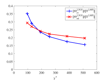
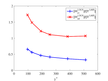
Figure 1: The norm of the deviation from the HIT tensor, $||\Theta_{ev}^{n,TCF}||/||T^{n,HIT}||$ (”+” symbols) and $||\Theta_{odd}^{n,TCF}||/||T^{n,HIT}||$ (”x” symbols) for $n=2$ (left panel) and $n=3$ (right panel), as a function of the distance from the wall $y^{+}$. The center of the channel is at $y^{+}\approx 1000$. The values shown here were obtained by processing the whole dataset. Using only half the dataset, as explained in Section II, would result in differences by no more than $5\%$.

Over the entire channel flow, the values of $\zeta$ in Eq. 7 differ from $1$ by no more than a few percent, even very close to the wall. The results for the norms of the deviations between the second and third order velocity gradient correlation tensors, and the isotropic predictions are presented in Fig. 1, which shows the values of $||\Theta_{ev}^{n,TCF}||$ and $||\Theta_{od}^{n,TCF}||$ ($n=1$, $2$), normalized by $||T^{n,HIT}||$, and measured at several values of $y^{+}$ in a region, $100\lesssim y^{+}\lesssim 500$ (the center of the channel is at $y^{+}\approx 1,000$). The range of values of $y^{+}$ shown corresponds essentially to the so-called logarithmic layer of the turbulent channel flow. In this region, the second (left panel) and third order (right panel) velocity gradient tensors deviate significantly more from the homogeneous and isotropic predictions, than the HSF flow, compare with Table 1.
Quantitatively, the deviations $\Theta^{2,TCF}$, normalized by $||T^{2,HIT}||$, shown in the left panel of Fig. 1, are of the order of $\approx 0.2$, and decay slightly when $y^{+}$ increases. The odd component $||\Theta_{od}^{2,TCF}||$ (”x” symbols) is larger than the even component, $||\Theta_{ev}^{2,TCF}||$ (”+” symbols) only for $y^{+}\gtrsim 200$. The norms of $\Theta^{3,TCF}$ divided by $||T^{3,HIT}||$ are shown in the right panel of Fig. 1. The norm of the odd part of the tensor $\Theta^{n,TCF}$ values of $||\Theta_{ov}^{n,TCF}||/||T^{n,HIT}||$ very close to the wall are much larger than those shown in Fig. 1, a simple consequence of the very strong influence of the boundary for $y^{+}\lesssim 100$.

Numerically, the norm of $\Theta_{od}^{3,TCF}$ normalized by $||T^{3,HIT}||$, $||\Theta_{od}^{3,TCF}||/||T^{3,HIT}||$, goes up to values $\approx 45$ at $y^{+}=1$. For $y^{+}\gtrsim 200$, in comparison, as shown in the right panel of Fig. 1 (”x” symbols), the values of $||\Theta_{od}^{3,TCF}||/||T^{3,HIT}||$ are approximately constant, and equal to $\approx 1.1$, a value roughly $\lesssim 2$ times larger than in HSF at $R_{\lambda}=145$. The values of $||\Theta_{ev}^{3,TCF}||/||T^{3,HIT}||$ (”+” symbols in the right panel of Fig. 1) vary in relative value similarly to those of $||\Theta_{od}^{3,TCF}||/||T^{3,HIT}||$. Close to the wall, at $y^{+}=1$, the measured value is $\approx 3$. In the log-layer, the values are $\approx 0.3-0.4$. We notice that the values shown in Fig. 1 are also roughly $\lesssim 2$ times larger than those found in the case of the HSF.

Fig. 1 and the discussion so far have been focused on the structure of the flow mostly in the log-layer of the channel, where the shear is significant. We end this subsection by noticing that, at the center of the channel, at $y^{+}\approx 1000$ (data not shown in Fig. 1), the odd components of the deviations $\Theta_{od}^{n,TCF}$ vanish. In fact, the value of $||\Theta_{od}^{n,TCF}||^{2}$ are comparable to (in fact, even smaller than) the values found when comparing a HIT DNS with the theoretical prediction, discussed in Subsection IV.1. In comparison, the values of $||\Theta_{ev}^{n,TCF}||^{2}$ are found to be significantly larger than those listed in Subsection IV.1: $||\Theta_{ev}^{2,TCF}||^{2}\approx 10^{-2}$ and $||\Theta_{ev}^{3,TCF}||^{2}\approx 8.\ 10^{-2}$.

V Comparison between Homogeneous shear flows and turbulent channel flow

Having explored in the previous section the magnitude of the deviations $\Theta^{2,3}$ in the case of HSF and TCF, we now ask how similar are the deviations of the second and third order velocity gradient tensor from their predicted form in the case of a HIT flow, Eq. (3) and (5). Specifically, to compare two flows, flow 1 and flow 2, we represent the tensor corresponding to flow 1, $\Theta_{ev,od}^{n,flow1}$ ($n=1$, $2$) as a form proportional to $\Theta_{ev,od}^{n,flow2}$, plus a discrepancy, $\Psi_{ev,od}^{n}$:

$$\Theta_{ev,od}^{n,flow1}=\mu_{ev,od}^{n}\Theta_{ev,od}^{n,flow2}+\Psi_{ev,od}^{n}$$ (8)

and choose $\mu_{ev,od}^{n}$ to minimize the norm of the error, $||\Psi_{ev,od}^{n}||$. The norm of $\Psi_{ev,od}^{n}$, normalized with $||\Theta_{ev,od}^{n,TCF}||$, provides a quantitative measure of how close are the deviations from isotropy in the two flows considered proportional to one another.

V.1 Comparison between two HSF at different Reynolds numbers

The comparison between the two turbulent HSF at $R_{\lambda}=145$ and $R_{\lambda}=120$, shows that the structures of the correlation tensors are in fact extremely similar. In the present subsection, we distinguish the deviations $\Theta_{ev,od}^{n,HSF}$ between the two flows by specifying the Reynolds numbers in the superscript: $\Theta_{ev,od}^{n,HSF;R120}$ ($\Theta_{ev,od}^{n,HSF;R145}$) corresponds to $R_{\lambda}=120$ ($R_{\lambda}=145$). The present analysis is based on the decomposition:

$$\Theta_{ev,od}^{n,HSF;R145}=\mu_{ev,od}^{n}\Theta_{ev,od}^{n,HSF;R120}+\Psi_{ev,od}$$ (9)

The values of the coefficients $\mu_{ev,od}^{n}$ and of the ratios $||\Psi_{ev,od}^{n}||/||\Theta_{ev,od}^{n,HSF;R145}||$, as defined by Eq. (9), are shown in Table 2. Numerically, the measured values of $\mu^{n}_{ev,od}$, are all less than $1$, in the range $0.7-0.8$. The small ratio between the norm of the discrepancy from the linear relation, $||\Psi_{ev,od}^{n}||$, and $||\Theta_{ev,od}^{n,HSF;R145}||$, see Table 2, suggest that the tensors are close to being proportional to each other. This justifies the observation that the values of $\mu_{ev,od}^{n}$ satisfy: $\mu^{n}_{ev,od}\approx||\Theta_{ev,od}^{n,HSF;R145}||/||\Theta_{ev,od}^{n,HSF;R120}||$ (values in Table 1). We notice that the values of $\mu$ are larger for $n=3$ than for $n=2$, which is consistent with the observation of a slower decay of the deviations from isotropy of the third order correlation functions already noticed Pumir (1996).

In the rest of the text, we will only consider the HSF at $R_{\lambda}=145$, and simply denote $\Theta_{ev,od}^{n,HSF}$ the deviation from the isotropic form of the tensor.

	$\mu_{ev}^{n}$	$||\Psi_{ev}^{n,HSF}||/||\Theta_{ev}^{n,HSF;R145}||$	$\mu_{od}^{n,HSF}$	$||\Psi_{od}^{n,HSF}||/||\Theta_{od}^{n,HSF;R145}||$
$n=2$	$0.72$	$0.078$	$0.80$	$0.051$
$n=3$	$0.77$	$0.14$	$0.86$	$0.080$

Table 2: Comparison between the two HSF at different Reynolds numbers. The notation refers to the Eq. 9 in the main text. The data shown here was obtained by processing the full dataset. The values of $\mu_{ev,od}^{n}$ obtained by processing only half the dataset (see Section II) differ by no more than $3\%$, whereas the small values of the norms of the discrepancy $||\Psi_{ev,od}^{n,HSF}||$ differ by $\approx 15\%$.

V.2 Comparison between TCF and HSF

The comparison between the HSF at $R_{\lambda}=145$ and the TCF, in the log-layer, are shown in Fig. 2, for the second (left part) and third (right part) correlation function of the velocity gradient tensor.
The values of $\mu$, upper part of Fig. 2, generally vary little in the range $200\lesssim y^{+}\lesssim 500$. This is consistent with the notion that in the log-layer, the properties of turbulence acquire some universal character. The values of $\mu^{n}_{ev,od}$ are all found to be $\approx 2$, pointing to a significantly larger deviation from isotropy in the case of TCF than of HSF Pumir et al. (2016a).
The relative discrepancies, $||\Psi_{ev,od}^{n}||/||\Theta_{ev,od}^{n,TCF}||$, shown in the bottom row of Fig. 2, are generally low, $\approx 0.15$, except for the even component associated with the third order correlation function of the velocity gradient, which is as high as $\approx 0.40$.

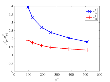
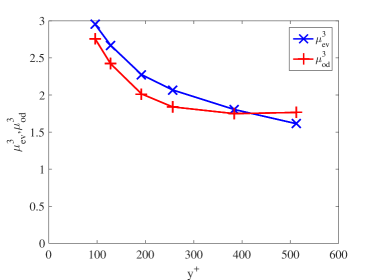
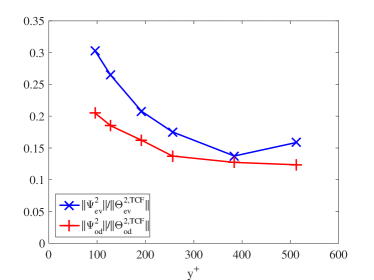
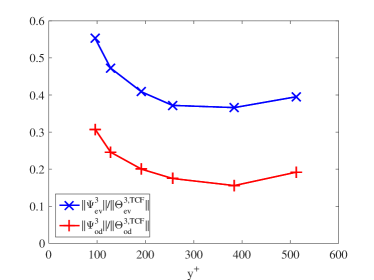
Figure 2: Comparison between $\Theta_{ev,od}^{n,TCF}$ in the log-layer of the TCF with $\Theta_{ev,od}^{n,HSF}$ ($R_{\lambda}=145$), for $n=2$ (left column) and $n=3$ (right column). The coefficient $\mu$, defined in Eq. (8), is shown in the upper row, and the norm of the discrepancy, $\Psi_{ev,od}^{n,HSF}$, divided by $||\Theta_{ev,od}^{n,TCF}||$ in the lower row. The errors are comparatively larger for $n=3$, especially for the even terms. The curves shown here were obtained by processing the full dataset. The values of $\mu$, obtained with only half the dataset (see Section  II) differ by no more than $5\%$ from those shown in the figure. The discrepancies $||\Psi_{ev,od}^{n,HSF}||$ also differ by less than $\approx 5\%$, except at $y^{+}=384$ and $y^{+}=512$, where $||\Psi_{od}^{3,HSF}||$ was found to differ by $15\%$ and $10\%$, respectively, from the indicated values.

VI Structure of the third order correlation tensor

Table 1 and Fig. 1 show that the largest deviations from isotropy are those measured by the third order velocity gradient correlation tensor, $T^{3,HSF}$ and $T^{3,TCF}$, the deviations from the HIT predictions being approximately twice smaller for the latter than for the former in the log-layer of the boundary layer. In this section, we focus on the largest components of $\Theta_{od,ev}^{3,TCF}$ and $\Theta_{od,ev}^{3,HSF}$.

Tables 3 and 4, discussed in more detail in the following subsections, list some of the components of the tensors $\Theta_{od,ev}^{3,HSF}$ and $\Theta_{od,ev}^{3,TCF}$ at $y^{+}=256$ and $y^{+}=512$, including the largest components measured numerically. As explained in Section II, we systematically compared the data shown below, obtained with the full dataset, with the values obtained with only half the dataset. In almost all cases where the absolute value of the listed component is larger than $0.1$, the results were found to differ in the second significant figure by no more than $\pm 1$, very rarely by $\pm 2$. The figure indicated for very small coefficients (less than $0.1$) were found in most cases to be unchanged when using half the dataset, or to differ by at most $1$, and by $2$ in only a very few cases. None of the signs of the quantities listed in the table was found to change when processing only half of the data. This analysis demonstrates that the data presented in Tables 3 and 4 is reliable.

VI.1 Structure of $\Theta_{od}^{3,TCF}$, $\Theta_{od}^{3,HSF}$

Table 3 lists most of the elements of the tensor $\Theta_{od}^{3,TCF}$ and $\Theta_{od}^{3,HSF}$. The components are presented per class of elements, deduced from one another by elementary symmetries. The components not shown in Table 3 can actually be derived from those shown by using incompressibility: $\partial_{a}u_{a}=0$; they turn out to be small.

Table 3 shows that the components of $\Theta_{od}^{3,TCF}$ vary relatively little in the TCF, over the range $256\lesssim y^{+}\lesssim 512$. This is consistent with the right panel of Fig. 1, which shows that the norm $||\Theta_{od}^{3,TCF}||$ is essentially constant over this range (see the curve with the ”x” symbols).

	Individual components of $\Theta_{od}^{3,HSF}$, $\Theta_{od}^{3,TCF}$ ($\times 10$)
Moments	$\langle(\partial_{2}u_{1})^{3}\rangle$	$\langle(\partial_{2}u_{1})^{2}(\partial_{1}u_{2})\rangle$	$\langle\partial_{2}u_{1}(\partial_{1}u_{2})^{2}\rangle$	$\langle(\partial_{1}u_{2})^{3}\rangle$
HSF	$2.83$	$-0.70$	$0.40$	$0.25$
$y^{+}=256$	$5.98$	$-1.31$	$0.85$	$-0.24$
$y^{+}=512$	$5.57$	$-1.29$	$0.91$	$-0.29$
Moments	$\langle\partial_{2}u_{1}(\partial_{1}u_{1})^{2}\rangle$	$\langle\partial_{2}u_{1}(\partial_{2}u_{2})^{2}\rangle$	$\langle\partial_{2}u_{1}(\partial_{3}u_{3})^{2}\rangle$	$\langle\partial_{1}u_{2}(\partial_{1}u_{1})^{2}\rangle$	$\langle\partial_{1}u_{2}(\partial_{2}u_{2})^{2}\rangle$	$\langle\partial_{1}u_{2}(\partial_{3}u_{3})^{2}\rangle$
$HSF$	$0.30$	$0.24$	$0.18$	$-0.07$	$-0.02$	$0.04$
$y^{+}=256$	$0.50$	$0.48$	$0.40$	$-0.07$	$-0.07$	$0.03$
$y^{+}=512$	$0.52$	$0.50$	$0.41$	$-0.10$	$-0.09$	$0.02$
Moments	$\langle\partial_{2}u_{1}\partial_{1}u_{1}\partial_{2}u_{2}\rangle$	$\langle\partial_{2}u_{1}\partial_{2}u_{2}\partial_{3}u_{3}\rangle$	$\langle\partial_{2}u_{1}\partial_{3}u_{3}\partial_{1}u_{1}\rangle$	$\langle\partial_{1}u_{2}\partial_{1}u_{1}\partial_{2}u_{2}\rangle$	$\langle\partial_{1}u_{2}\partial_{2}u_{2}\partial_{3}u_{3}\rangle$	$\langle\partial_{1}u_{2}\partial_{3}u_{3}\partial_{1}u_{1}\rangle$
$HSF$	$-0.18$	$-0.06$	$-0.12$	$0.06$	$-0.04$	$0.006$
$y^{+}=256$	$-0.30$	$-0.16$	$-0.22$	$0.10$	$-0.02$	$-0.01$
$y^{+}=512$	$-0.31$	$-0.18$	$-0.22$	$0.11$	$-0.02$	$-0.004$
Moments	$\langle\partial_{2}u_{1}(\partial_{1}u_{3})^{2}\rangle$	$\langle\partial_{2}u_{1}(\partial_{3}u_{1})^{2}\rangle$	$\langle\partial_{2}u_{1}\partial_{1}u_{3}\partial_{3}u_{1}\rangle$	$\langle\partial_{1}u_{2}(\partial_{1}u_{3})^{2}\rangle$	$\langle(\partial_{1}u_{2})(\partial_{3}u_{1})^{2}\rangle$	$\langle(\partial_{1}u_{2})\partial_{1}u_{3}\partial_{3}u_{1}\rangle$
HSF	$0.33$	$1.06$	$-0.25$	$-0.01$	$-0.21$	$0.03$
$y^{+}=256$	$0.50$	$1.84$	$-0.41$	$-0.01$	$-0.38$	$0.09$
$y^{+}=512$	$0.60$	$1.72$	$-0.42$	$-0.02$	$-0.34$	$0.09$
Moments	$\langle\partial_{2}u_{1}(\partial_{2}u_{3})^{2}\rangle$	$\langle\partial_{2}u_{1}(\partial_{3}u_{2})^{2}\rangle$	$\langle\partial_{2}u_{1}\partial_{2}u_{3}\partial_{3}u_{2}\rangle$	$\langle\partial_{1}u_{2}(\partial_{2}u_{3})^{2}\rangle$	$\langle(\partial_{1}u_{2})(\partial_{3}u_{2})^{2}\rangle$	$\langle(\partial_{1}u_{2})\partial_{2}u_{3}\partial_{3}u_{2}\rangle$
HSF	$0.87$	$-0.20$	$-0.06$	$-0.51$	$0.19$	$0.24$
$y^{+}=256$	$1.51$	$-0.11$	$-0.08$	$-0.86$	$0.04$	$0.34$
$y^{+}=512$	$1.60$	$0.03$	$-0.15$	$-0.83$	$0.01$	$0.36$
Moments	$\langle\partial_{3}u_{2}\partial_{2}u_{2}\partial_{1}u_{3}\rangle$	$\langle\partial_{2}u_{3}\partial_{2}u_{2}\partial_{1}u_{3}\rangle$	$\langle\partial_{3}u_{2}\partial_{2}u_{2}\partial_{3}u_{1}\rangle$	$\langle\partial_{2}u_{3}\partial_{2}u_{2}\partial_{3}u_{1}\rangle$
HSF	$-0.18$	$0.14$	$0.32$	$-0.29$
$y^{+}=256$	$-0.30$	$0.29$	$0.48$	$-0.48$
$y^{+}=512$	$-0.27$	$0.24$	$0.45$	$-0.41$
Moments	$\langle\partial_{3}u_{2}\partial_{3}u_{3}\partial_{1}u_{3}\rangle$	$\langle\partial_{2}u_{3}\partial_{3}u_{3}\partial_{1}u_{3}\rangle$	$\langle\partial_{3}u_{2}\partial_{3}u_{3}\partial_{3}u_{1}\rangle$	$\langle\partial_{2}u_{3}\partial_{3}u_{3}\partial_{3}u_{1}\rangle$
HSF	$0.17$	$-0.18$	$-0.25$	$0.29$
$y^{+}=256$	$0.24$	$-0.33$	$-0.37$	$0.49$
$y^{+}=512$	$0.22$	$-0.29$	$-0.34$	$0.40$

Table 3: A subset of the components of the third order velocity gradient correlation tensor with an odd number of indices $1$ and $2$ (all terms with an odd number of $3$ are zero by symmetry). The values are shown for the HSF at $R_{\lambda}=145$, and for the TCF at $y^{+}=256$ and $y^{+}=512$, which includes all the largest values measured. With a few notable exceptions, these values do not vary too much with $y^{+}$ in the range considered, and are roughly $\approx 1.8$ times larger than in the HSF.

Among all the large terms listed in Table 3, the largest values in HSF are smaller than the corresponding ones in TCF at $y^{+}=256$ and $y^{+}=512$ by a factor $\approx 1.8$. This is manifestly consistent with the value of $\mu^{3}_{od}$ shown in Fig. 2. The ratios between the components in TCF and in HSF deviate much more significantly from $\approx 1.8$ for some of the weaker components. Sign changes between HSF and TCF components are observed for the $\langle(\partial_{1}u_{2})^{3}\rangle$ and $\langle\partial_{2}u_{1}(\partial_{3}u_{2})^{2}\rangle$, which manifestly point to differences between the two flows.

The largest of all the components shown in Table 3 is $\langle(\partial_{2}u_{1})^{3}\rangle$, which exceeds any of the other components by a factor $\approx 3$. We recall that the term $\partial_{2}u_{1}$ is the fluctuation around the mean shear, $dU_{1}/dx_{2}$, and that the third moment $\langle(\partial_{2}u_{1})^{3}\rangle$ has been used to investigate anisotropy in turbulent shear flows Pumir and Shraiman (1995); Pumir (1996); Pumir et al. (2016a).
Particularly significant is the sign of $\langle(\partial_{2}u_{1})^{3}\rangle$, which is identical to the sign of the mean shear, $dU_{1}/dx_{2}$. This reflects the (partial) expulsion of the velocity gradients from large regions of the flow Pumir and Shraiman (1995); Pumir et al. (2016a). In the related problem of a passive scalar, $\theta$, in the presence of a mean scalar gradient, $\langle\theta\rangle=\mathbf{G}\cdot\mathbf{x}$, it is well-established that the distribution of the scalar gradient, $\nabla\theta$, has a sharp peak at $\nabla\theta=0$. This points to a sharp expulsion of the gradients, which are manifested by the presence of large regions of space over which the scalar is approximately constant. These regions are separated by narrow regions, where large scalar jumps form Sreenivasan (1991); Holzer and Siggia (1994); Pumir (1994), implying the formation of large gradients, which in turn contribute to the odd moments of $\mathbf{G}\cdot(\nabla\theta)$, in particular to the skewness, which is determiend by the large scale gradient, $\mathbf{G}$. This effect is also seen, although in a weaker form, in numerical simulations of HSF or TCF. In the flows considered here, the mean velocity gradient, $dU_{1}/dx_{2}$ is always positive, and the positive sign of $\langle(\partial_{2}u_{1})^{3}\rangle$ can be interpreted as a result of very large positive fluctuations of $\partial_{2}u_{1}$, resulting from extended regions of space where $\partial_{2}(U_{1}+u_{1})$ is relatively small, separated by regions where $\partial_{2}(U_{1}+u_{1})$ is much larger than the mean, $\partial_{2}U_{1}$.

The picture sketched above would suggest that quantities of the form $\langle\partial_{2}u_{1}(\partial_{a}u_{b}\partial_{a}u_{b})\rangle$, could be dominated by positive fluctuations of $\partial_{2}u_{1}$, suggesting a positive value of the moment $\langle\partial_{2}u_{1}(\partial_{a}u_{b})^{2}\rangle$. This is true for all terms with $a=b$, and for all terms with $a\neq b$, with the exception of the term $\langle\partial_{2}u_{1}(\partial_{3}u_{2})^{2}\rangle$ in HSF. This term turns out to be relatively small in TCF, and even to becomes positive in TCF at $y^{+}=512$. The same considerations suggest that terms of the form $\langle\partial_{2}u_{1}(\partial_{a}u_{b}\partial_{b}u_{a})\rangle$ have the same sign as $\langle(\partial_{a}u_{b}\partial_{b}u_{a})\rangle$, which is negative when $a\neq b$. This is consistent with the expressions listed in Table 3. Last, we also notice that terms of the form $\langle\partial_{2}u_{1}(\partial_{a}u_{a}\partial_{b}u_{b})\rangle$ for $a\neq b$ all have negative signs, as implied by the above considerations. Obtaining a more quantitative parametrization of terms of the form $\langle\partial_{2}u_{1}(\partial_{a}u_{b}\partial_{c}u_{d})\rangle$ in terms of $\langle\partial_{a}u_{b}\partial_{c}u_{d}\rangle$ does not appear to be simply feasible.

Whereas the terms containing one or more terms of the form $\partial_{2}u_{1}$ are the dominant ones, and have a sign that can be understood with the help of the simple considerations above, the third moments containing $\partial_{1}u_{2}$ are generally smaller than those with $\partial_{2}u_{1}$. In TCF, the first set of components in Table 3 indicates that the sign of $\langle(\partial_{2}u_{1})^{3-p}(\partial_{1}u_{2})^{p}\rangle$ is $(-1)^{p}$, generally indicating a sign difference in the contributions of $\partial_{2}u_{1}$ (which tend to be positive) and of $\partial_{1}u_{2}$ (which tend to be negative). This empirical rule accounts for the sign of most of the terms of the form $\langle\partial_{1}u_{2}(\partial_{a}u_{b})^{2}\rangle$ in the table, with a few exceptions. The difference in sign of $\langle(\partial_{1}u_{2})^{3}\rangle$ between TCF and HSF points to the quantitative limitation of the empirical observation that $(\partial_{1}u_{2})$ generally provides a negative contribution to the moments investigated here.

VI.2 Structure of $\Theta_{ev}^{3,TCF}$, $\Theta_{ev}^{3,HSF}$

	Individual components of $\Theta_{ev}^{3,HSF}$, $\Theta_{ev}^{3,TCF}$ ($\times 10$)
Moments	$\langle(\partial_{1}u_{1})^{3}\rangle$	$\langle(\partial_{2}u_{2})^{3}\rangle$	$\langle(\partial_{3}u_{3})^{3}\rangle$
HSF	$-0.18$	$0.06$	$0.03$
$y^{+}=256$	$-0.37$	$0.18$	$-0.007$
$y^{+}=512$	$-0.28$	$0.15$	$-0.02$
Moments	$\langle(\partial_{1}u_{1})(\partial_{1}u_{2})^{2}\rangle$	$\langle(\partial_{1}u_{1})(\partial_{1}u_{3})^{2}\rangle$	$\langle(\partial_{2}u_{2})(\partial_{2}u_{1})^{2}\rangle$	$\langle(\partial_{2}u_{2})(\partial_{2}u_{3})^{2}\rangle$	$\langle(\partial_{3}u_{3})(\partial_{3}u_{1})^{2}\rangle$	$\langle(\partial_{3}u_{3})(\partial_{3}u_{2})^{2}\rangle$
HSF	$-0.26$	$-0.27$	$0.22$	$0.11$	$0.14$	$-0.06$
$y^{+}=256$	$-0.44$	$-0.49$	$0.58$	$0.41$	$0.21$	$-0.21$
$y^{+}=512$	$-0.38$	$-0.40$	$0.48$	$0.31$	$0.15$	$-0.17$
Moments	$\langle(\partial_{1}u_{1})(\partial_{2}u_{1})^{2}\rangle$	$\langle(\partial_{1}u_{1})(\partial_{3}u_{1})^{2}\rangle$	$\langle(\partial_{2}u_{2})(\partial_{1}u_{2})^{2}\rangle$	$\langle(\partial_{2}u_{2})(\partial_{3}u_{2})^{2}\rangle$	$\langle(\partial_{3}u_{3})(\partial_{1}u_{3})^{2}\rangle$	$\langle(\partial_{3}u_{3})(\partial_{2}u_{3})^{2}\rangle$
HSF	$-0.14$	$-0.14$	$0.13$	$0.12$	$0.05$	$0.01$
$y^{+}=256$	$-0.12$	$-0.25$	$0.11$	$0.27$	$-0.05$	$-0.05$
$y^{+}=512$	$-0.10$	$-0.18$	$0.17$	$0.23$	$-0.04$	$-0.08$
Moments	$\langle\partial_{2}u_{1}\partial_{1}u_{1}\partial_{1}u_{2}\rangle$	$\langle\partial_{3}u_{1}\partial_{1}u_{1}\partial_{1}u_{3}\rangle$	$\langle\partial_{1}u_{2}\partial_{2}u_{2}\partial_{2}u_{1}\rangle$	$\langle\partial_{3}u_{2}\partial_{2}u_{2}\partial_{2}u_{3}\rangle$	$\langle\partial_{1}u_{3}\partial_{3}u_{3}\partial_{3}u_{1}\rangle$	$\langle\partial_{2}u_{3}\partial_{3}u_{3}\partial_{3}u_{2}\rangle$
HSF	$0.14$	$0.14$	$-0.13$	$-0.08$	$-0.06$	$0.03$
$y^{+}=256$	$0.26$	$0.24$	$-0.24$	$-0.26$	$-0.07$	$0.13$
$y^{+}=512$	$0.23$	$0.19$	$-0.20$	$-0.20$	$0.06$	$0.10$
Moments	$\langle\partial_{1}u_{1}(\partial_{2}u_{3})^{2}\rangle$	$\langle\partial_{1}u_{1}(\partial_{3}u_{2})^{2}\rangle$	$\langle\partial_{2}u_{2}(\partial_{1}u_{3})^{2}\rangle$	$\langle\partial_{2}u_{2}(\partial_{3}u_{1})^{2}\rangle$	$\langle\partial_{3}u_{3}(\partial_{1}u_{2})^{2}\rangle$	$\langle\partial_{3}u_{3}(\partial_{2}u_{1})^{2}\rangle$
HSF	$-0.12$	$-0.08$	$0.21$	$-0.08$	$0.13$	$-0.09$
$y^{+}=256$	$-0.33$	$-0.36$	$0.55$	$0.02$	$0.35$	$-0.48$
$y^{+}=512$	$-0.21$	$-0.04$	$0.45$	$0.02$	$0.26$	$-0.40$
Moments	$\langle\partial_{1}u_{2}\partial_{2}u_{3}\partial_{1}u_{3}\rangle$	$\langle\partial_{1}u_{2}\partial_{3}u_{2}\partial_{3}u_{1}\rangle$	$\langle\partial_{1}u_{2}\partial_{3}u_{2}\partial_{1}u_{3}\rangle$	$\langle\partial_{2}u_{1}\partial_{1}u_{3}\partial_{2}u_{3}\rangle$	$\langle\partial_{2}u_{1}\partial_{3}u_{1}\partial_{3}u_{2}\rangle$	$\langle\partial_{2}u_{1}\partial_{3}u_{1}\partial_{2}u_{3}\rangle$
HSF	$0.01$	$-0.02$	$-0.08$	$-0.08$	$0.10$	$0.19$
$y^{+}=256$	$-0.10$	$-0.09$	$-0.30$	$-0.02$	$0.27$	$0.40$
$y^{+}=512$	$-0.05$	$-0.08$	$-0.23$	$-0.02$	$0.25$	$0.23$

Table 4: A subset of the components of the deviations of the third order velocity gradient correlation tensor with an even number of all indices, from the corresponding isotropic tensor. The values are shown for the HSF at $R_{\lambda}=145$, and for the TCF at $y^{+}=256$ and $y^{+}=512$. As it was the case for the tensors $\Theta_{od}^{3,HSF}$ and $\Theta_{od}^{3,TCF}$, see Table. 3. The values for the TCF vary more with $y^{+}$ than in the case of the odd terms, consistent with Fig. 1. The ratio between the values in TCF and in HSF is roughly $1.8$.

Table 4 lists several groups of coefficients of $\Theta_{ev}^{3,HSF}$ and $\Theta_{ev}^{3,TCF}$, which include all the largest elements of $\Theta_{ev}^{3,HSF}$. Namely, we separated all the non-zero elements of $\Theta_{ev}^{3,HIT}$ in several classes of identical elements, which can be deduced from one another by a permutation of the indices $(1,2,3)$ (see the Appendix), and selected those for which one of the elements of this class is larger than $1/100$. Table 4 systematically compares the results obtained for HSF with those obtained for TCF, for $y^{+}=256$ and $y^{+}=512$. The values of $\Theta_{ev}^{3,TCF}$ generally show a larger variation over the range $256\lesssim y^{+}\lesssim 512$, compared to the variation found for the components of $\Theta_{od}^{3,TCF}$ shown in Table 3. This is consistent with Fig. 1, which shows a small, but visible variation of $||\Theta_{ev}^{3,TCF}||$ over the corresponding range of values of $y^{+}$.

Overall, Table 4 indicates that, consistent with the value of $\mu_{ev}^{3}$ reported in Fig. 2, the ratios between many of the coefficients shown in the table are close to $\approx 1.8$. This is particularly true for the largest elements of the tensor. This proportionality relation does not hold so well for some of the smaller coefficients. Some of the coefficients of $\Theta_{ev}^{3,HSF}$ differ from those of $\Theta_{ev}^{3,TCF}$ even by their signs. The differences between the components of $\Theta_{ev}^{3,TCF}$ and $\approx\mu_{ev}\Theta_{ev}^{3,HSF}$, tends to be systematically larger than their counterparts for the odd components of $\Theta$. This certainly accounts for the fact that $||\Psi_{ev}||$ is roughly twice larger than $||\Psi_{od}||$, see the lower right panel of Fig. 2.

VII Discussion

To recapitulate, we have systematically investigated the structure of the second and third order correlation of the velocity gradient tensor in elementary shear flows: HSF and TCF in the logarithmic region. The comparison with the exact form of the tensors in the case of HIT provides an unambiguous way to measure how the flow deviates from isotropy. In particular, our analysis allows us to identify corrections to the HIT form of the tensor. Although the magnitude of these corrections depends on the flow (TCF or HSF), the overall structures are very comparable. It is worth stressing here that the largest discrepancy between the measured velocity tensors, and its HIT counterpart comes from the odd contribution to the $n=3$ velocity gradient correlations (see the right panels of Fig. 1). The corresponding structure is the one that turns out to be the most similar, in TCF and in HSF (see the lower right panel of Fig. 2).

Interestingly, the largest of all the components of the odd contribution to the third order velocity derivative tensor is the one that corresponds to the third order moment of $\partial_{2}u_{1}$, the derivative of the streamwise component of the velocity in the normal direction. This quantity had been investigated numerically Pumir and Shraiman (1995); Pumir (1996); Schumacher and Eckhardt (2000); Pumir et al. (2016a) and experimentally Garg and Warhaft (1998); Shen and Warhaft (2000), based on a possible analogy with the observation of a skewness of the scalar gradient, which remains of order ${\cal O}(1)$, independent of $R_{\lambda}$, in the presence of a mean scalar gradient Sreenivasan (1991); Holzer and Siggia (1994); Pumir (1994); Tong and Warhaft (1994); Shraiman and Siggia (2000); Warhaft (2000). While the scalar analogy was providing an enticing theoretical motivation, suggesting experimentally measurable quantities, the results of the present study demonstrate that the third moment of $\partial_{2}u_{1}$ is indeed the most sensitive third order moment to the presence of shear. Consistent with the ratio of an overall factor $\approx 1.7$ between the odd part of the third order velocity gradient tensor in the TCF for $200\lesssim y^{+}\lesssim 600$ and HSF, the skewness of $\partial_{2}u_{1}$ was found to $\approx 1.07$ in TCF, and $0.65$ in HSF Pumir et al. (2016a).

As it turns out, the Reynolds numbers in the log-layer of the TCF and in the HSF are comparable, $R_{\lambda}\approx 150$. Comparing TCF and HSF at comparable Reynolds numbers leads already to interesting conclusions. It has already been observed that the difference in the magnitude of the third moment of the velocity gradient tensors is presumably due to the very different forcing. As suggested by standard phenomenology, the notion that the flow integral scale in TCF a distance $x_{2}$ away from the wall is $\approx x_{2}$ Tennekes and Lumley (1983); Pope (2000) suggests that the effect of the boundary may be felt throughout the log-region of the TCF. On the other hand, the skewness of $\partial_{2}u_{1}$ in HSF is known to decrease, albeit weakly, with $R_{\lambda}$ (like $R_{\lambda}^{-\alpha}$, with $\alpha\approx 0.5$). For obvious reasons, it would be interesting to study the dependence of the low-order velocity gradient tensors considered here as a function of the Reynolds number. Although the even tensor $\Theta_{ev}^{3,HSF}$ and $\Theta_{ev}^{3,TCF}$ are generally smaller than their odd counterparts in the Reynolds numbers considered here, it remains to be understood whether and how these terms decay as a function of the Reynolds number. The limited comparison between $||\Theta_{ev}^{3,HSF}||$ at the two Reynolds numbers may suggest a faster decay of $||\Theta_{ev}^{3,HSF}||$ than the one observed for $||\Theta_{od}^{3,HSF}||$. Convincing evidence can only be provided by investigating HSF at higher Reynolds numbers. Although it is to be expected that a systematic group theoretic analysis of the problem may be helpful Biferale and Procaccia (2005), especially in the case of a homogeneous flow, a precise calculation remains to be done. The decomposition of the tensors $\Theta^{n,flow}$ as a sum of an even and of an odd part merely separates spherical harmonics with even and odd eigenvalues $l$ of the angular momentum operator. It is generally expected that the decay of the tensors will be dominated by the lowest angular momentum ($l=1$ for the odd terms, and $l=2$ for the even ones). In the inhomogeneous case of TCF, where the role of the boundary may persist even far away from the boundary, whether the skewness will stay constant, or ultimately decay as in the HSF case, remains to be investigated.

It is enticing to compare the structure of the velocity gradient correlation tensor, uncovered in the case of HSF and TCF in the logarithmic layer, with the structure obtained by shearing a homogeneous isotropic flow. In practice, this can be done by applying the transformation induced by the mean shear Townsend (1970) to a numerical solution of the Navier-Stokes equations, and deducing the velocity gradient correlation tensors. This can be done in practice by using a simulation in a triply periodic domain (see Pumir (1994) for details) and applying a stretching in the range $0\leq St\leq 1$. The deviations $\Theta$ of the second and third order velocity gradient correlation tensors from the form expected in a homogeneous, isotropic flow, defined using Eq. (7), grows linearly with the amount of stretching. The structure of $\Theta$, however, does not indicate any close similarity with the one found in HSF and TCF.

The observation that the tensors of order $n=2$ and $n=3$ in HIT are completely characacterized by only one invariant makes our analysis unambiguous. Higher order tensors in HIT involve more than 1 dimensional quantity, which may significantly complicate the analysis. As recently observed Pumir et al. (2016a), however, in the case $n=4$, the ratios between the 4 invariants quantities that characterize the velocity gradient correlations Siggia (1981) seem to be independent of the flow. This property, which remains to be more thoroughly understood, may make the analysis tractable also for the $n=4$ order tensor. Such an analysis may provide new insight on the production and formation of very large gradients in the flows. The available experimental data in the case $n>4$ Shen and Warhaft (2002) points to a rich structure, which deserves further attention.

Appendix

As done in Siggia (1981), it is convenient to decompose the velocity gradient tensor $A_{ab}=\partial_{a}u_{b}$, where $1\leq a\leq 3$ and $1\leq b\leq 3$ refer to the spatial coordinates, into a symmetric and antisymmetric parts: $s_{ab}=(A_{ab}+A_{ba})/2$, and $\omega_{a}=\epsilon_{abc}A_{bc}$, so

$$\partial_{a}u_{b}=s_{ab}+\epsilon_{abc}\omega_{c}/2$$ (10)

The third moment $\langle s_{ab}s_{cd}s_{ef}\rangle$ can be expressed as a function of a single dimensional quantity, $\langle tr(s^{3})\rangle$, and of the (Kronecker) $\delta$-tensor. Using the isotropy of the tensor $s$, one can write, in full generality:

$$\langle s_{ab}s_{cd}s_{ef}\rangle = A\delta_{ab}\delta_{cd}\delta_{ef}$$ (11)

$$+ B\Bigl{(}\delta_{ab}(\delta_{ce}\delta_{df}+\delta_{cf}\delta_{de})+\delta_{cd}(\delta_{ae}\delta_{bf}+\delta_{af}\delta_{be})+\delta_{ef}(\delta_{ac}\delta_{bd}+\delta_{ad}\delta_{bc})\Bigr{)}$$

$$+ C\Bigl{(}\delta_{ac}\delta_{de}\delta_{fb}+\delta_{ac}\delta_{df}\delta_{eb}+\delta_{ad}\delta_{ce}\delta_{fb}+\delta_{ad}\delta_{cf}\delta_{eb}$$

$$~{}~{}+\delta_{bc}\delta_{de}\delta_{fa}+\delta_{bc}\delta_{df}\delta_{ea}+\delta_{bd}\delta_{ce}\delta_{fa}+\delta_{bd}\delta_{cf}\delta_{ea}\Bigr{)}$$

Constraints on the constants $A$, $B$ and $C$ can be found by expressing the incompressibility of the velocity field: $\sum_{a=1}^{3}s_{aa}=0$:

$$\sum_{a=1}^{3}\langle s_{aa}s_{cd}s_{ef}\rangle = 3A\delta_{cd}\delta_{ef}+B\Bigl{(}3(\delta_{ce}\delta_{df}+\delta_{cf}\delta_{de})+4\delta_{cd}\delta_{ef}\Bigr{)}+4C\Bigl{(}\delta_{de}\delta_{fc}+\delta_{ce}\delta_{df}\Bigr{)}$$

$$= (3A+4B)\delta_{cd}\delta_{ef}+(3B+4C)(\delta_{de}\delta_{cf}+\delta_{ce}\delta_{df})$$

which immediately imposes that $3A+4B=3B+4C=0$, and thus allows us to express $\langle s_{ab}s_{cd}s_{ef}\rangle$ with only one number. To fully determine the tensor, we evaluate the trace of $s^{3}$: $\langle tr(s^{3})\rangle=\sum_{a,b,c}\langle s_{ab}s_{bc}s_{ca}\rangle$

$$\langle tr(s^{3})\rangle=3A+36B+66C$$ (13)

which leads to the final expression:

$$\langle s_{ab}s_{cd}s_{ef}\rangle = \frac{2}{35}\langle tr(s^{3})\rangle\times\Bigl{[}\frac{4}{3}\delta_{ab}\delta_{cd}\delta_{ef}$$ (14)

$$- [\delta_{ab}(\delta_{ce}\delta_{df}+\delta_{cf}\delta_{de})+\delta_{cd}(\delta_{ae}\delta_{bf}+\delta_{af}\delta_{be})+\delta_{ef}(\delta_{ac}\delta_{bd}+\delta_{ad}\delta_{bc})]$$

$$+ \frac{3}{4}(\delta_{ac}\delta_{de}\delta_{fb}+\delta_{ac}\delta_{df}\delta_{eb}+\delta_{ad}\delta_{ce}\delta_{fb}+\delta_{ad}\delta_{cf}\delta_{eb}$$

$$~{}~{}+\delta_{bc}\delta_{de}\delta_{fa}+\delta_{bc}\delta_{df}\delta_{ea}+\delta_{bd}\delta_{ce}\delta_{fa}+\delta_{bd}\delta_{cf}\delta_{ea})\Bigr{]}$$

In addition to the tensor $\langle s_{ab}s_{cd}s_{ef}\rangle$, one has also to consider quantities such as $\langle s_{ab}s_{cd}\omega_{e}\rangle$, $\langle s_{ab}\omega_{c}\omega_{d}\rangle$ and $\langle\omega_{a}\omega_{b}\omega_{c}\rangle$. Under reflection, $(x,y,z)\rightarrow(-x,-y,-z)$, the tensor $s$ remains unchanged, whereas $\omega\rightarrow-\omega$. Thus, in a flow that is invariant under reflection, only terms with an even number of values of $\omega_{a}$ are non zero. The only term to estimate is therefore $\langle s_{ab}\omega_{c}\omega_{d}\rangle$. As before, symmetry considerations impose that:

$$\langle s_{ab}\omega_{c}\omega_{d}\rangle=D\delta_{ab}\delta_{cd}+E(\delta_{ac}\delta_{bd}+\delta_{ad}\delta_{bc})$$ (15)

Incompressibility ($\sum_{1\leq a\leq 3}s_{aa}=0$) leads to: $3D+2E=0$. The tensor can be conveniently expressed in terms of stretching, $\langle\mathbf{\omega}\cdot\mathbf{s}\cdot\mathbf{\omega}\rangle$:

$$\langle s_{ab}\omega_{c}\omega_{d}\rangle=\langle\mathbf{\omega}\cdot\mathbf{s}\cdot\mathbf{\omega}\rangle\Bigl{(}-\frac{1}{15}\delta_{ab}\delta_{cd}+\frac{1}{10}(\delta_{ac}\delta_{bd}+\delta_{ad}\delta_{bc})\Bigr{)}$$ (16)

Remains to express the full tensor $\langle\partial_{a}u_{b}\partial_{c}u_{d}\partial_{e}u_{f}\rangle$. This can be done by using Eq. (10):

$$\langle\partial_{a}u_{b}\partial_{c}u_{d}\partial_{e}u_{f}\rangle = \langle(s_{ab}+\epsilon_{abA}\omega_{A}/2)(s_{cd}+\epsilon_{cdB}\omega_{B}/2)(s_{ef}+\epsilon_{efC}\omega_{C}/2)\rangle$$ (17)

$$= \langle s_{ab}s_{cd}s_{ef}\rangle+\frac{1}{4}\epsilon_{cdB}\epsilon_{efC}\langle s_{ab}\omega_{B}\omega_{C}\rangle$$

$$+ \frac{1}{4}\epsilon_{efC}\epsilon_{abA}\langle s_{cd}\omega_{C}\omega_{A}\rangle+\frac{1}{4}\epsilon_{abA}\epsilon_{cdB}\langle s_{ef}\omega_{A}\omega_{B}\rangle$$

By substituting the expressions for $\langle s_{ab}s_{cd}s_{ef}\rangle$ and $\langle s_{ab}\omega_{A}\omega_{B}\rangle$, Eq. (14,16) into Eq. (17) gives:

$$\langle\partial_{a}u_{b}\partial_{c}u_{d}\partial_{e}u_{f}\rangle=\frac{2}{35}\langle tr(s^{3})\rangle\times\Bigl{[}\frac{4}{3}\delta_{ab}\delta_{cd}\delta_{ef}$$ (18)

$$- [\delta_{ab}(\delta_{ce}\delta_{df}+\delta_{cf}\delta_{de})+\delta_{cd}(\delta_{ae}\delta_{bf}+\delta_{af}\delta_{be})+\delta_{ef}(\delta_{ac}\delta_{bd}+\delta_{ad}\delta_{bc})]$$

$$+ \frac{3}{4}(\delta_{ac}\delta_{de}\delta_{fb}+\delta_{ac}\delta_{df}\delta_{eb}+\delta_{ad}\delta_{ce}\delta_{fb}+\delta_{ad}\delta_{cf}\delta_{eb}$$

$$~{}~{}+\delta_{bc}\delta_{de}\delta_{fa}+\delta_{bc}\delta_{df}\delta_{ea}+\delta_{bd}\delta_{ce}\delta_{fa}+\delta_{bd}\delta_{cf}\delta_{ea})\Bigr{]}$$

$$+ \frac{1}{20}\langle\mathbf{\omega}\cdot\mathbf{s}\cdot\mathbf{\omega}\rangle\times\Bigl{[}-\frac{1}{3}\delta_{ef}(\delta_{ac}\delta_{bd}-\delta_{ad}\delta_{bc})-\frac{1}{3}\delta_{cd}(\delta_{ae}\delta_{bf}-\delta_{af}\delta_{be})-\frac{1}{3}\delta_{ab}(\delta_{ce}\delta_{df}-\delta_{cf}\delta_{de})$$

$$+ \frac{1}{2}(\epsilon_{abe}\epsilon_{cdf}+\epsilon_{abf}\epsilon_{cde})+\frac{1}{2}(\epsilon_{abc}\epsilon_{efd}+\epsilon_{abd}\epsilon_{efc})+\frac{1}{2}(\epsilon_{cda}\epsilon_{efb}+\epsilon_{cdb}\epsilon_{efa})\Bigr{]}$$

The two constants involved in the expression Eq. (18) are in fact connected by the well known identity:

$$\sum_{a,b,c=1}^{3}\langle\partial_{a}v_{b}\partial_{b}v_{c}\partial_{c}v_{a}\rangle=0$$ (19)

which results from the homogeneity of the flow Betchov (1956). Elementary algebraic manipulations lead to:

$$\sum_{a,b,c=1}^{3}\langle\partial_{a}v_{b}\partial_{b}v_{c}\partial_{c}v_{a}\rangle=\langle tr(s^{3})\rangle+\frac{3}{4}\langle\mathbf{\omega}\cdot\mathbf{s}\cdot\mathbf{\omega}\rangle$$ (20)

hence to the well known identity:

$$\langle\mathbf{\omega}\cdot\mathbf{s}\cdot\mathbf{\omega}\rangle=-\frac{4}{3}\langle tr(s^{3})\rangle$$ (21)

Substituting Eq. (21) into Eq. (18) immediately leads to Eq. (5).

It is very elementary to see that only components of $T^{3,HIT}_{abcdef}$ with an even number of indices $1$, $2$ and $3$ can be non-zero. The components of $T^{3,HIT}$ which involve only one of the three indices are $T^{3,HIT}_{aaaaaa}=\frac{8}{105}$. Those which involve two indices, $a$ and $b$ ($a\neq b$) are one of the possible forms: $T^{3,HIT}_{aabbbb}=-\frac{4}{105}$, $T^{3,HIT}_{aaabab}=\frac{16}{315}$, $T^{3,HIT}_{abbaba}=\frac{16}{315}$ and $T^{3,HIT}_{aaabba}=\frac{2}{315}$. Last, the components of $T^{3,HIT}$ which involve 3 diffent indices, $a$, $b$ and $c$, with $a\neq b$, $b\neq c$ and $a\neq c$ are of the form: $T^{3,HIT}_{aabbcc}=\frac{8}{105}$, $T^{3,HIT}_{aabcbc}=-\frac{32}{315}$, $T^{3,HIT}_{aabccb}=-\frac{4}{315}$, $T^{3,HIT}_{abbcca}=-\frac{2}{35}$ and $T^{3,HIT}_{abbcac}=-\frac{8}{105}$.

References

- Betchov (1956) R. Betchov, “An inequality concerning the production of vorticity in isotropic turbulence,” J. Fluid Mech. 1, 497–504 (1956).
- Tennekes and Lumley (1983) H. Tennekes and J. L. Lumley, A first course on turbulence, 9th ed. (The MIT Press, 1983).
- Batchelor and Townsend (1949) G. K. Batchelor and A. A. Townsend, “The nature of turbulent motion at large wave-numbers,” Proc. R. Soc. Lond. A 199, 238–255 (1949).
- Frisch (1995) U. Frisch, Turbulence, 1st ed. (Cambridge University Press, 1995).
- Siggia (1981) E. D. Siggia, “Invariants for the one-point vorticity and strain rate correlation functions,” Phys Fluids 24, 1934–1936 (1981).
- Kolmogorov (1941) A. N. Kolmogorov, “The local structure of turbulence in incompressible viscous fluid for very large reynolds numbers,” Dokl Akad Nauk SSSR 30, 301–305 (1941).
- Pope (2000) S. B. Pope, Turbulent flows (Cambridge University Press, 2000).
- Champagne et al. (1970) F. H. Champagne, V. G. Harris, and S. Corrsin, “Experiments on nearly homogeneous turbulent shear flows,” J. Fluid Mech. 41, 81–139 (1970).
- Garg and Warhaft (1998) S. Garg and Z. Warhaft, “On small scale statistics in a simple shear flow,” Phys Fluids 10, 662–673 (1998).
- Pumir and Shraiman (1995) A. Pumir and B. Shraiman, “Persistent small scale anisotropy in homogeneous shear flows,” Phys Rev. Let. 75, 3114–3117 (1995).
- Pumir et al. (2016a) A. Pumir, H. Xu, and E. D. Siggia, “Small-scale anisotropy in turbulent boundary layers,” J. Fluid Mech. 804, 5–23 (2016a).
- Pumir (1996) A. Pumir, “Turbulence in homogeneous shear flows,” Phys. Fluids 8, 3112–3127 (1996).
- Mizuno and Jimenez (2013) Y. Mizuno and J Jimenez, “Wall turbulence without walls,” J Fluid Mech 723, 429–455 (2013).
- Dong (2016) S. Dong, Coherent structures in statistically-stationary homogeneous shear turbulence, Ph.D. thesis, Universidad Politécnica de Madrid (2016).
- Vreman and Kuerten (2014a) A. W. Vreman and J. G. M. Kuerten, “Statistics of spatial derivatives of velocity and pressure in turbulent channel flow,” Phys. Fluids 27, 084103 (2014a).
- Shen and Warhaft (2000) X. Shen and Z. Warhaft, “The anisotropy of the small scale structure in high reynolds number () turbulent shear flow,” Phys Fluids 12, 2976–2989 (2000).
- Sreenivasan (1991) K. R. Sreenivasan, “On local isotropy of passive scalars in turbulent flows,” Proc. R. Soc. Lond. A 434, 165–182 (1991).
- Holzer and Siggia (1994) M. Holzer and E. D. Siggia, “Turbulent mixing of a passive scalar,” Phys. Fluids 6, 1820–1837 (1994).
- Pumir (1994) A. Pumir, “A numerical study of the mixing of a passive scalar in three-dimensions in the presence of a mean gradient,” Phys. Fluids 6, 2118–2132 (1994).
- Tong and Warhaft (1994) C. Tong and Z. Warhaft, “On passive scalar derivative statisics in grid turbulence,” Phys. Fluids 6, 2165–2176 (1994).
- Warhaft (2000) Z. Warhaft, “Passive scalars in turbulent flows,” Ann. Rev. Fluid Mech. 32, 203–240 (2000).
- Batchelor (1946) G. K. Batchelor, “The theory of axisymmetric turbulence,” Proc. R. Soc. Lond. A 186, 480–502 (1946).
- Graham et al. (2014) J. Graham, M. Lee, N. Malaya, R. D. Moser, G. Eyink, and C. Meneveau, “The JHU turbulence database: Turbulent channel flow data set,” (2014), http://turbulence.pha.jhu.edu/docs/README-CHANNEL.pdf.
- Li et al. (2008) Y. Li, M. Wan, Y. Yang, R. Burns, C. Meneveau, R. Burns, S. Chen, A. Szalay, and Eyink G., “A public turbulence database cluster and application to study lagrangian evolution of velocity increments in turbulence,” J. Turbulence 9, 133–166 (2008).
- Sekimoto et al. (2016) A. Sekimoto, S. Dong, and J. Jimenez, “Direct numerical simulation of statistically stationary and homogeneous shear turbulence and its relation to other shear flows,” Phys Fluids 28, 035101 (2016).
- Pumir et al. (2016b) A. Pumir, H. Xu, E. Bodenschatz, and R. Grauer, “Single-particle motion and vortex stretching in three-dimensional turbulent flows,” Phys. Rev. Lett. 116, 124502 (2016b).
- Landau and Lifshitz (1959) L. D. Landau and E. M. Lifshitz, Fluid Mechanics, 1st ed. (Pergamon Press, 1959).
- Vreman and Kuerten (2014b) A. W. Vreman and J. G. M. Kuerten, “Comparison of direct numerical simulation databases of turbulent channel flow at Re,” Phys. Fluids 26, 105102 (2014b).
- Corrsin (1958) S. L. Corrsin, Local isotropy in turbulent shear flows, Tech. Rep. (National Advisory Committee for Aeronautics, 1958).
- Lumley (1967) J. L. Lumley, “Similarity and the thurbulent energy spectrum,” Phys Fluids 10, 855–858 (1967).
- Schumacher and Eckhardt (2000) J. Schumacher and B. Eckhardt, “On statistically stationary homogeneous shear turbulence,” EPL 52, 627–632 (2000).
- Shraiman and Siggia (2000) B. Shraiman and E. D. Siggia, “Scalar turbulence,” Nature 405, 639–646 (2000).
- Biferale and Procaccia (2005) L. Biferale and I. Procaccia, “Anisotropy in turbulent flows and in turbulent transport,” Phys. Reports 414, 43–164 (2005).
- Townsend (1970) A. A. Townsend, “Entrainment and the structure of turbulent flow,” J. Fluid Mech. 41, 13–46 (1970).
- Shen and Warhaft (2002) X. Shen and Z. Warhaft, “Longitudinal and transverse structure functions in sheared and unsheared wind turbulence,” Phys. Fluids 14, 370–381 (2002).