Wigner Distributions of Quarks and Gluons

Abstract:

We present a recent calculation of Wigner distributions of quarks and gluons for a quark target state dressed with a gluon, using overlaps of light-front wave functions.

1 Introduction

In quantum mechanics, Wigner distributions [1] can be interpreted as semi-classical objects giving a combined position and momentum space description of a system. Wigner distributions of quarks and gluons [2, 3] in a nucleon are of interest recently as they are related to generalized transverse momentum dependent parton distributions(GTMDs) that give the most general information about the momentum and spin correlations of quarks and gluons. There is also the possibility of accessing the quark and gluon orbital angular momentum through Wigner distributions or GTMDs [3, 4, 5]. If one integrates the Wigner distributions over transverse momentum, one obtains impact parameter dependent parton distributions, which are Fourier transform of generalized parton distributions (GPDs); integration over transverse position relates them on the other hand to transverse momentum dependent parton distributions (TMDs). Quark Wigner distributions have been investigated in several model calculations [3, 6, 7, 8]. Most of the models do not have a gluonic degree of freedom, and thus gluon Wigner distributions are less explored apart from the small $x$ region. Gluon Wigner distributions, or the unintegrated gluon correlators have been introduced and discussed in the context of small $x$ physics in [9] for diffractive vector meson production, and in [10] for Higgs production at Tevatron and LHC. Operator definitions of gluon GTMDs for a spin $1/2$ target are given in [11]. Gluon GTMDs and Wigner distributions have been studied at small $x$ in deeply virtual Compton scattering (DVCS) [12] and in hard diffractive dijet production in lepton-hadron scattering [13]. In [14] gluon Wigner and Husimi distributions are discussed. Husimi distributions are positive definite, unlike Wigner distributions, however, upon integration over $b_{\perp}$ they do not reduce to TMDs. Recently, we have investigated the quark and gluon Wigner distributions taking the target to be a quark dressed with a gluon [15, 16]. This may be thought of as a simple spin $1/2$ composite state having a gluonic degree of freedom. As a continuation of our project, we have improved the numerical convergence of the result to remove an artificial cutoff dependence, as well as extended to transverse polarization. Here, we report on some of our recent results [18, 19].

2 Wigner Distributions in a dressed quark model

The Wigner distributions of quarks are defined as the Fourier transform of the quark-quark correlators : [17, 3]

$$\rho^{[\Gamma]}({\boldsymbol{b}}_{\perp},{\boldsymbol{k}}_{\perp},x,s,s^{\prime})=\int\frac{d^{2}\Delta_{\perp}}{(2\pi)^{2}}e^{-i{\boldsymbol{\Delta}}_{\perp}.{\boldsymbol{b}}_{\perp}}W_{s\,s^{\prime}}^{[\Gamma]}({\boldsymbol{\Delta}}_{\perp},{\boldsymbol{k}}_{\perp},x)$$ (1)

where ${\boldsymbol{b}_{\perp}}$ is the impact parameter conjugate to ${\boldsymbol{\Delta}}_{\perp}$, which is the momentum transfer of the state in the transverse direction. The quark-quark correlator $W^{[\Gamma]}$ for the GTMDs are defined at a fixed light-front time as

$$W_{s\,s^{\prime}}^{[\Gamma]}({\boldsymbol{\Delta}}_{\perp},{\boldsymbol{k}}_{\perp},x) = \int\!\!\frac{dz^{-}d^{2}{\boldsymbol{z}}_{\perp}}{2(2\pi)^{3}}e^{ik.z}\Big{\langle}p^{+},\frac{{\boldsymbol{\Delta}}_{\perp}}{2},s^{\prime}\Big{|}\overline{\psi}(-\frac{z}{2})\Omega\Gamma\psi(\frac{z}{2})\Big{|}p^{+},-\frac{{\boldsymbol{\Delta}}_{\perp}}{2},s\Big{\rangle}\Big{|}_{z^{+}=0}$$ (2)

The average four-momentum of the target state is given by $P={1\over 2}(p^{\prime}+p)$, the momentum transfer $\Delta=p^{\prime}-p$ in the transverse direction. $s$($s^{\prime}$) is the helicity of the initial (final) target state. The average four momentum of the quark is $k$, with $k^{+}=xP^{+}$, where $x$ is the longitudinal momentum fraction of the parton. $\Omega$ is the gauge link for color gauge invariance. We use light-cone gauge and take the gauge link to be unity.

The Wigner distribution of the gluon can be defined as [17, 3]

$$xW_{\sigma,\sigma^{\prime}}(x,{k}_{\perp},{b}_{\perp}) = \int\frac{d^{2}{\Delta}_{\perp}}{(2\pi)^{2}}e^{-i{\Delta}_{\perp}.{b}_{\perp}}\int\frac{dz^{-}d^{2}z_{\perp}}{2(2\pi)^{3}p^{+}}e^{ik.z}$$ (3)

$$\times \Big{\langle}p^{+},-\frac{{\Delta}_{\perp}}{2},\sigma^{\prime}\Big{|}\Gamma^{ij}F^{+i}\Big{(}-\frac{z}{2}\Big{)}F^{+j}\Big{(}\frac{z}{2}\Big{)}\Big{|}p^{+},\frac{{\Delta}_{\perp}}{2},\sigma\Big{\rangle}\Big{|}_{z^{+}=0}$$

$$F^{+i}=\partial^{+}A^{i}-\partial^{i}A^{+}+gf^{abc}A^{+}A^{i}$$ (4)

$\Gamma^{ij}=\delta^{ij}$ for unpolarized distribution. Wigner distribution for gluons need two gauge links for gauge invariance. As in the quark case, we use light-cone gauge and take the gauge links to be unity. $\sigma$ and $\sigma^{\prime}$ are the helicities of the target state, for unpolarized distribution $W_{UU}$, we average over the helicity of the target. Instead of a proton target, we take the state to be a quark dressed with a gluon.

A dressed quark state can be expanded in Fock space as

$$\Big{|}p^{+},{\boldsymbol{p}}_{\perp},s\Big{\rangle} = \Phi^{s}(p)b^{\dagger}_{s}(p)|0\rangle+\sum_{s_{1}s_{2}}\int\frac{dp_{1}^{+}d^{2}p_{1}^{\perp}}{\sqrt{16\pi^{3}p_{1}^{+}}}\int\frac{dp_{2}^{+}d^{2}p_{2}^{\perp}}{\sqrt{16\pi^{3}p_{2}^{+}}}\sqrt{16\pi^{3}p^{+}}\delta^{3}(p-p_{1}-p_{2})$$ (5)

$$\times\Phi^{s}_{s_{1}s_{2}}(p;p_{1},p_{2})b^{\dagger}_{s_{1}}(p_{1})a^{\dagger}_{s_{2}}(p_{2})|0\rangle$$

The two-particle light-front wave function LFWF can be written in terms of the boost-invariant LFWF as

$$\sqrt{P^{+}}\Phi(p;p_{1},p_{2})=\Psi(x_{i},{\boldsymbol{q}}_{i}^{\perp})$$ (6)

The two-particle LFWF can be calculated in light-front Hamiltonian perturbation theory. The Wigner distributions for the dressed quark state for different combinations of polarizations of the target and the probed quark are expressed in terms of overlaps of the light-front wave functions. The single particle sector of the Fock space component plays an important role when $x=1$. Out of the $16$ leading twist Wigner distributions that one can define, in our model we obtain only $8$ independent non-zero functions. They are calculated analytically using LFWFs and the Fourier transform is done numerically. Unpolarized gluon Wigner is calculated in the same approach. Here we present some of our numerical results.

3 Numerical Results

In all plots we have used Levin’s method to do the numerical integration, which is a reliable method for oscillatory integrand. We have used the upper limit of the $\Delta_{\perp}$ integration to be $\Delta_{max}=20~{}\mathrm{GeV}$, and the results are independent of this cutoff. We choose the mass of the quark to be $m=0.33~{}GeV$. In all plots we have integrated over $x$.

Fig. 1(a) shows the plot of $\rho_{UU}$ in $b$ space. This gives the distribution of an unpolarized quark in an unpolarized target state. Fig. 1(b) shows the plot of $\rho_{UL}$ in $b$ space for a fixed value of the $k_{\perp}$. In this model, $\rho_{UL}=\rho_{LU}$. This Wigner distribution is related to the orbital angular momentum of the quark. A dipole structure is seen similar to chiral quark soliton model and constituent quark model [3]. In Fig. 2(a) we have plotted $\rho^{x}_{UT}$, which gives the distribution of transversely polarized quark in an unpolarized target; quark polarization in the $x$ direction. Here we also observe a dipole structure. TMD limit of $\rho_{UT}$ is the Boer-Mulders function. As we have taken the gauge link to be unity, we cannot calculate the T-odd distributions, and Boer-Mulders function is zero in our model. The behaviour in $b$ space is similar to spectator model [6]. In Fig. 2(b) we have shown the gluon Wigner distribution $W_{UU}$, which is the distribution of an unpolarized gluon in an unpolarized dressed quark. As mentioned above, each gluon Wigner distribution needs two gauge links for gauge invariance. Depending on whether it is a $++$ or $+-$ gauge link combination, it is called a Weizsacker-Williams type or dipole type gluon distribution. In [13] it was shown that both of them give the same orbital angular momentum distribution of the gluon. As we mentioned, in our model, we have taken the gauge links to be unity in light-cone gauge. The gluon distribution has a positive peak at the center of the $b$ space.

(a)   (b)

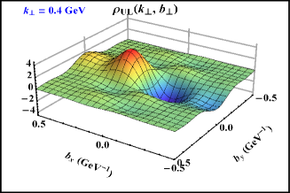
Figure 1: 3D plots of Wigner distributions $\rho_{UU}({\boldsymbol{k}}_{\perp},{\boldsymbol{b}}_{\perp})$ and $\rho_{UL}({\boldsymbol{k}}_{\perp},{\boldsymbol{b}}_{\perp})$ at $\Delta_{max}=20~{}\mathrm{GeV}$.

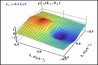
(a)   (b)

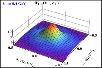
Figure 2: 3D plots of Wigner distributions $\rho^{x}_{UT}({\boldsymbol{k}}_{\perp},{\boldsymbol{b}}_{\perp})$ and gluon Wigner distribution $W_{UU}({\boldsymbol{k}}_{\perp},{\boldsymbol{b}}_{\perp})$ at $\Delta_{max}=20~{}\mathrm{GeV}$.

4 Conclusion

We presented a recent calculation of the Wigner distributions of quarks and gluons in a dressed quark target model. This represents a composite spin $1/2$ state with a gluonic degree of freedom. The Wigner distributions are expressed in terms of overlaps of LFWFs and using their analytic form one can calculate them. Better convergence of the results is obtained using Levin’s method of integration, that removes the dependence on an artificial cutoff on $\Delta_{\perp}$. We presented the Wigner distributions for unpolarized, longitudinally polarized and transversely polarized quark in an unpolarized target state. We also presented the unpolarized gluon Wigner distributions.

5 Acknowledgement

AM would like to thank the organizers of ”XXV International Workshop on Deep-Inelastic Scattering and Related Subjects” at the University of Birmingham, UK for invitation.

References

- [1] E. P. Wigner, Phys. Rev. 40, 749 (1932).
- [2] X. D. Ji, Phys. Rev. Lett. 91, 062001 (2003).
- [3] C. Lorce and B. Pasquini, Phys. Rev. D 84, 014015 (2011).
- [4] Y. Hatta, Phys. Lett. B 708, 186 (2012).
- [5] P. Hagler, A. Mukherjee and A. Schafer, Phys. Lett. B 582, 55 (2004).
- [6] T. Liu and B. Q. Ma, Phys. Rev. D 91, 034019 (2015).
- [7] D. Chakrabarti, T. Maji, C. Mondal and A. Mukherjee, Phys. Rev. D 95, No. 7, 074028 (2017).
- [8] D. Chakrabarti, T. Maji, C. Mondal, A. Mukherjee, Eur. Phy. J C 76, no. 7, 409 (2016).
- [9] A. D. Martin, M. Ryskin, T. Teubner, Phys. Rev. D 62, 014022 (2000).
- [10] V. A. Khoze, A. D. Martin, M. Ryskin, Eur. Phy. J. C 14, 525 (2000).
- [11] C. Lorce and B. Pasquini, J. High Energy Phys. 09 (2013) 138.
- [12] Y. Hatta, B-W. Xiao, F. Yuan, arXiv. 1703.02085 [hep-ph].
- [13] Y. Hatta, Y. Nakagawa, F. Yuan, Y. Zhao, arXiv : 1612.02445 [hep-ph].
- [14] Y. Hagiwara, Y. Hatta, T. Ueda, Phys. Rev. D 94, No. 9, 094036 (2016).
- [15] A. Mukherjee, S. Nair and V. K. Ojha, Phys. Rev. D 90, 014024 (2014).
- [16] A. Mukherjee, S. Nair and V. K. Ojha, Phys. Rev. D 91, 054018 (2015).
- [17] S. Meissner, A. Metz and M. Schlegel, J. High Energy Phys. 08 (2009) 056.
- [18] J. More, A. Mukherjee, S. Nair, Phys. Rev. D 95, No. 7, 074039 (2017).
- [19] J. More, A. Mukherjee, S. Nair, In Preparation.