A Radial Time Projection Chamber for $\alpha$ detection in CLAS at JLab

Abstract

A new Radial Time Projection Chamber (RTPC) was developed at the Jefferson Laboratory to track low-energy nuclear recoils to measure exclusive nuclear reactions, such as coherent deeply virtual Compton scattering and coherent meson production off ⁴He. In 2009, we carried out these measurements using the CEBAF Large Acceptance Spectrometer (CLAS) supplemented by the RTPC positioned directly around a gaseous ⁴He target, allowing a detection threshold as low as 12 MeV for ⁴He. This article discusses the design, principle of operation, calibration methods and performances of this RTPC.

Keywords: Time projection chamber, gas electron multipliers, alpha particles, DVCS, Nuclear physics.

1 Introduction

Until recently, the Thomas Jefferson National Accelerator Facility, in Newport News, Virginia, USA, has provided high power electron beams of up to 6 GeV energy and 100$\%$ duty factor to three experimental Halls (A, B, C) simultaneously. The CEBAF Large Acceptance Spectrometer (CLAS) [1], located in Hall-B, was based on a superconducting toroidal magnet and composed of several sub-detectors. Figure 1 shows a three dimensional representation of the baseline CLAS spectrometer:

• Three regions of Drift Chambers (DC) for the tracking of charged particles [2].

• Superconducting toroidal magnet to bend the trajectories of charged particles, thus allowing momentum measurement with the DC tracking information.

• Threshold Cherenkov Counters (CC) for electron identification at momenta $<2.7$ GeV/c [3].

• Scintillation Counters (SC) to identify charged hadrons by measuring their time of flight [4].

• Electromagnetic Calorimeters (EC) for identification of electrons, photons and neutrons [5].

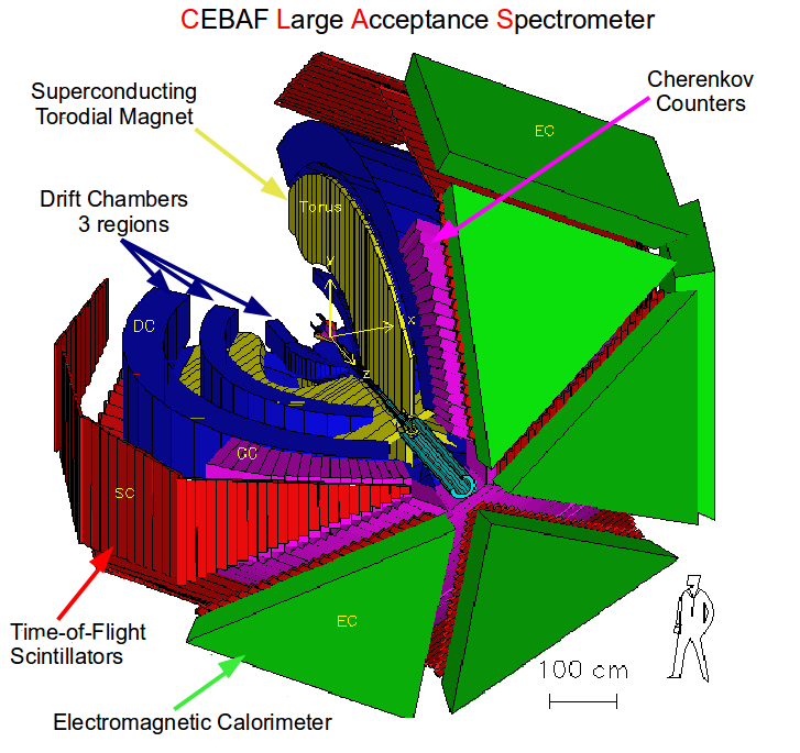
Figure 1: A three dimensional representation of the baseline CLAS setup. The full description is given in the text.

For certain experiments the base CLAS system was complemented with ancillary detectors. For example, the measurement of the Deeply Virtual Compton Scattering (DVCS) process ($eH\rightarrow e^{\prime}H^{\prime}\gamma$, where $H$ is a nucleon or nucleus) necessitates an upgrade of the photon detection system. Indeed, with a 6 GeV electron beam, the majority of DVCS photons are produced at very forward angles, where the acceptance of the EC was poor. To extend the detection range, an inner calorimeter (IC) was built for the E01-113 experiment in 2005 [6]. The IC was constructed from 424 lead-tungstate (PbWO₄) crystals, covering polar angles between 5^∘ and 15^∘ [7]. To protect the CLAS detector and the IC from the large flux of the low energy Møller electrons, a 5 T solenoid magnet was placed around the target to shield the detectors. To detect recoiling $\alpha$ particles from the coherent DVCS on Helium, a new radial time projection chamber (RTPC) was developed to track low energy nuclear fragments. The solenoid field was used to bend tracks and measure momentum of particles in the RTPC. The CLAS detector supplemented with both IC and RTPC was used in 2009 during a three months experimental run [8, 9] with a longitudinally polarized, 130 nA and 6.064 GeV electron beam incident on a gaseous ⁴He target.

The original design of the RTPC was developed for the BoNuS experiment at Jefferson Lab which took data with CLAS in 2005 [10]. Significant improvements were made to the RTPC mechanical structure and fabrication technique that both increased the acceptance and reduced the amount of material in the path of the outgoing particles. Moreover, the data acquisition electronic was improved to increase the event readout rate. The enhanced design, used in the 2009 DVCS experiment, is described in section 2 of this article. The data acquisition system is described in section 3, the calibration methods in section 4 and the tracking algorithm in section 5. Finally, the overall performances of the RTPC are described in section 6.

2 RTPC design

With a 6 GeV incident electron energy, the recoiling ⁴He nuclei from coherent DVCS have an average momentum around 300 MeV/c (12 MeV kinetic energy). Such low energy $\alpha$ particles are stopped very rapidly, so the RTPC was designed to be as close as possible to the target and fit inside the 230 mm diameter shell and cryostat wall of the solenoid magnet bore of CLAS.

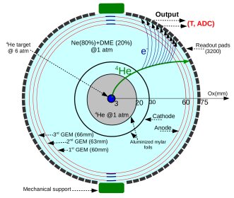
Figure 2: Schematic drawing of the CLAS RTPC in a plane perpendicular to the beam direction. See text for description of the elements.

The new CLAS RTPC is a 250 mm long cylinder of 158 mm diameter, leaving just enough room to fit pre-amplifiers between the RTPC outer shell and the solenoid. The electric field is directed perpendicularly to the beam direction, such that drifting electrons are pushed away from the beam line. These electrons are amplified by three layers of semi-cylindrical gas electron multipliers (GEM) [11] and detected by the readout system on the external shell of the detector as illustrated in Figure 2. The RTPC is segmented into two halves with independent GEM amplification systems that cover about 80% of the azimuthal angle.

We detail here the different regions shown in Figure 2 starting from the beam line towards larger radius:

• The 6 atm ⁴He target extends along the beamline forming the detector central axis. It is a 6 mm diameter Kapton straw with a 27 µm wall of 292 mm length such that its entrance and exit 15 µm aluminum windows are placed outside of the detector volume. The detector and the target are placed in the center of the solenoid, 64 cm upstream of the CLAS center.

• The first gas gap covers the radial range from 3 mm to 20 mm. It is filled with ⁴He gas at 1 atm to minimize secondary interactions from Møller electrons scattered by the beam. This region is surrounded by a 4 µm thick window made of grounded aluminized Mylar.

• The second gas gap region extends between 20 mm and 30 mm and is filled with the gas mixture of 80$\%$ neon (Ne) and 20$\%$ dimethyl ether (DME). This region is surrounded by a 4 µm thick window made of aluminized Mylar set at $-4260$ V to serve as the cathode.

• The drift region is filled with the same Ne-DME gas mixture and extends from the cathode to the first GEM, 60 mm away from the beam axis. The electric field in this region is perpendicular to the beam and averages around 550 V/cm.

• The electron amplification system is composed of three GEMs located at radii of 60, 63 and 66 mm. The first GEM layer is set to $\Delta V=1620$ V relative to the cathode foil and then each subsequent layer is set to a lower voltage relative to the previous to obtain a strong ($\sim$1600 V/cm) electric field between the GEM foils. A 275 V bias is applied across each GEM for amplification.

• The readout board has an internal radius of 69 mm and collects charges after they have been multiplied by the GEMs. Pre-amplifiers are plugged directly on its outer side and transmit the signal to the data acquisition electronics.

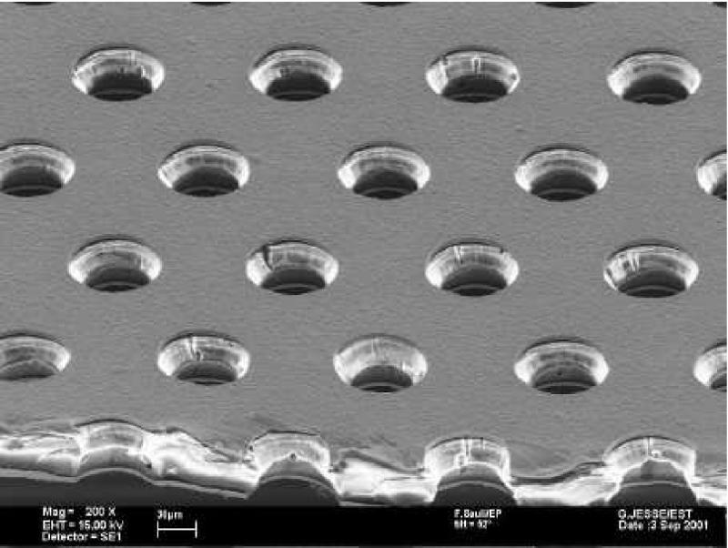
Figure 3: Image of a typical GEM foil similar to the one used for our RTPC [11].

The GEM technology has been chosen for the flexibility of the GEM foils, which can be easily used to produce a curved amplification surface. Also, GEMs are known to have relatively low spark rate [12], which is important when trying to detect highly ionizing slow nuclei that deposit large amount of energy. The GEMs for this RTPC are made from a Kapton insulator layer, 50 µm thick, sandwiched between two 5 µm copper layers. The mesh of each GEM layer is chemically etched with 50 µm diameter holes with double-conical shapes as illustrated in Figure 3. The potential difference applied between the two copper layers of the GEM creates a very strong electric field in each hole leading to high ionization and amplification.

The drift gas used in the experiment is a 80%-20% Ne-DME mixture. This choice has been made in order to balance the energy deposit, which is critical for proper particle identification, with a reasonable Lorentz angle. Calculations using the MAGBOLTZ program [13] showed that with the 5 T solenoidal magnetic field, we would have a Lorentz angle of about 23^∘ with this gas mixture.

The main structural improvement compared to the 2005 RTPC [10] was to obtain a better support structure for the GEM foils. In the previous version, the RTPC was essentially composed of two independent half-cylinder separated by their own structures. In this design, the installation of the GEMs was not very practical and wrinkles were visible on the GEM surfaces. To allow for a better installation and, at the same time, keep the mechanical structure out of the drift volume, the present design is based on self supporting GEM cylinder. We realized these cylinders by using fiber glass rings glued to each end of the GEM foils in order to install them independently in the RTPC after gluing and soldering operations. The rigidity of the GEM foils was enough for the structure to be self-supporting and only the upstream end of the cylinder was fixed to the mechanical support structure. This design only left a light fiberglass ring in the downstream end, reducing to a minimum secondary interactions.

3 Readout System

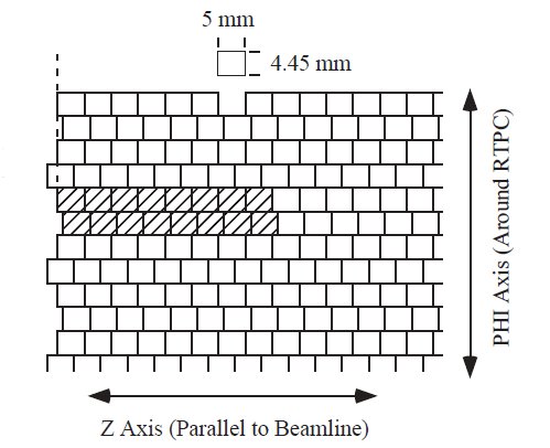
Figure 4: A schematic representation of the readout pads. The shaded sixteen pads are a group of pads that are connected to the same pre-amplifier.

The RTPC electron collection system had 3200 readout pads. These elements were located at the end of the amplification region, 69 mm from the central axis. Figure 4 illustrates the configuration of the 5 by 4.45 mm pads, where the shift between the rows was implemented to reduce aliasing. Each half of the RTPC had 40 rows and 40 columns of pads. The shaded region in Figure 4 shows how pads were grouped to 16 channels pre-amplifier boards. The pre-amplifier boards, already employed in the BoNuS RTPC [10], serve the dual purpose of inverting the RTPC signals polarity – from negative to positive – to match the requirements of the subsequent readout system, and driving signals through the 6 m long ribbon cable that connects to the readout system.

The readout system was an upgraded version of the original BoNuS RTPC system [10], based on ALICE-TPC front end electronic boards (FECs) [14]. Each FEC hosted 128 channels, providing amplification and digitization of the input signals. For each event, 100 samples/channel were digitized by the ALTRO ASIC [15], operated at 10 MHz sampling frequency. In order to reduce the data size, the system was operated in zero-suppression mode, keeping data from $N_{PRE}=3$ samples before threshold crossing on the rising edge to $N_{POST}=3$ samples after threshold crossing on the falling edge. The threshold level was set on each channel just above the noise level.

A new custom backplane was developed to connect FECs to the Readout Control Unit (RCU) [16], allowing fast (200 MB/s) communication between the boards. The RCU board, used to distribute the trigger signal to different FECs and read data, was equipped with a fast optical link for data transferring to the main event builder. These features, together with the “block-transfer” readout mode making use of the FECs multi-event buffer, allowed to reach a significantly higher readout-rate compared to the original BoNuS system. During the 2009 run, the system was successfully operated with a DAQ rate of 3.1 kHz and a live time of 70 %, for a luminosity of about $10^{34}$ cm${}^{-2}\cdot$s^-1 and a beam energy of 6.064 GeV, to be compared with the 500 Hz obtained with the first BoNuS detector at similar run conditions.

During data reconstruction, the acquired samples were processed to obtain, for each readout pad, the accumulated charge (ADC) and the pulse time (T). Since pulse time was obtained as the time-stamp of the first sample above threshold, referred to the trigger time, the resolution was equivalent to the ALTRO sampling time of 100 ns.

4 Calibration

The timing information collected from each signal is used to infer the origin of the ionization electrons, from which we reconstruct the trajectory of the initial particle. The strength of these signals, recorded in ADC units, is then used to reconstruct the deposited energy per unit of length ($\small{\frac{dE}{dX}}$) which, together with the momentum calculated from the trajectory, enabled the particle identification.

In this section we will detail the methods used to calibrate the drift time, drift paths and gains of the detector. The drift paths were initially calculated using the MAGBOLTZ [13] program, then refined using data to account for variations of the run conditions. The initial MAGBOLTZ calibration was improved through several iterations of the data driven process described below, with each time an increasing number of tracks reconstructed in the RTPC justifying a new iteration. The figures presented in this section are the ones obtained while performing the last iteration of this calibration process. We assume cylindrical symmetry in the chamber for the calibration of the drift parameters, such that do not depend on the azimuthal angle $\phi$.

4.1 Maximum Drift Time Parametrization

The first step in the calibration is to fix the maximum drift time ($T_{max}$) that an electron can arrive on the detection plane. This value is highly dependent on the gas mixture composition, as well as the electric and magnetic field experienced by the drift electrons. The maximum time corresponds to electrons released close to the cathode, which are the furthest from the readout pads as illustrated in Figure 5. Note that the minimum time is not calibrated, as we use the trigger time for it ($T_{min}=15$), and that the time unit is the ALTRO sampling time of 100 ns.

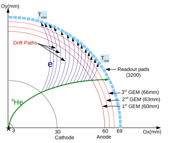
Figure 5: A schematic drawing of a ⁴He track (in green) traversing the drift region, with the drift paths followed by the electrons (in blue).

In order to experimentally determine the value of $T_{max}$, we analyze the time profile of hits from identified good tracks, as presented in Figure 6. We can clearly observe the expected dropping edge and define $T_{max}$, as the time at which the distribution passes below half the maximum number of hits in the histogram. This value was measured in bins along the 200 mm RTPC’s length to take into account variations in the electric and magnetic field. We show this result for one experimental run in Figure 7.

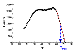
Figure 6: Time distribution of the hits in one z-bin along the RTPC in one experimental run.

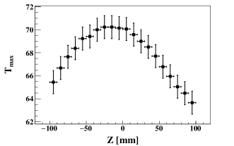
Figure 7: Maximum time of collected hits as a function of the track position on the $z$-axis for one experimental run.

Figure 8 shows the $T_{max}$ values for individual runs (approximately 2 hours long). We observe significant change of $T_{max}$ before and after run 61600, while variations within these periods are around 2%. This is likely due to non-perfect experimental conditions, in particular possible contamination of our gas mixture. We indeed increase the gas flow around that time due to a small leak in the RTPC. While our gas system was kept slightly over atmospheric pressure to limit contamination from air or other external gases, it is likely that this leak was the source of modification of the drift velocity.

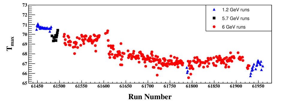
Figure 8: $T_{max}$ versus the experimental run numbers.

To take this effects into account, we parametrized the maximum drift time as a function of both the position along the beam axis and the run number. These functions were extracted for the entire data set and implemented in the track reconstruction code for the next steps of calibration and track reconstruction.

4.2 Drift Path Calibration

The drift path is the trajectory followed by the electrons released through ionization in the gas. We initially calculated them with MAGBOLTZ [13], but this calculation requires knowledge of the detector’s geometry, of the gas mixture composition, and of the electric and magnetic fields over the whole volume of the detector. As we seen in the previous section, the conditions in the chamber were changing over time. Moreover, the 4 µm foil used as a cathode is easily deformed, such that we expect the geometrical accuracy to be only of a few millimeters, also impacting our knowledge of the electric field. These problems, already encountered for the BoNuS RTPC calibration [10], motivated the acquisition of specific calibration runs. These were taken with a lower energy electron beam (1.204 and 1.269 GeV) to enhance the cross section of the elastic scattering ($e^{4}$He$\rightarrow e^{4}$He). In this process, the measurement of the electron kinematics allows to calculate the kinematics of the Helium nucleus. By comparing the calculated momentum and angle of the recoil alpha particle to the measurement in the RTPC, we tuned the drift paths independently of our knowledge of the chamber’s conditions.

Based on the kinematics of the electrons in the calibration data, we generated the Helium nucleus in our RTPC GEANT4 simulation [17]. Then, we compared the calculated GEANT4 trajectory of the Helium nuclei to the hits measured in the chamber. To perform the drift path extraction, we made a first approximation assuming a linear dependence between the radius of emission of the charge and its time of detection, and then refined our result accounting for the curvature of the drift path. The curvature was small enough, such that the process converged already on the second iteration.

At the end of the extraction procedure, the azimuthal difference between the detection pad and the ionization point ($\Delta\phi$) was extracted as a function of time. In Figure 9, we show the resulting data points for one bin in z-coordinate of the RTPC, where the drift path is easily identified and eventually fitted for implementation in our reconstruction code.

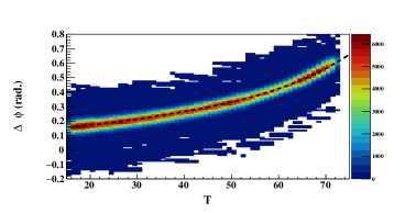
Figure 9: $\Delta\phi$ versus T distribution for tracks from one bin in longitudinal position along the RTPC. The black line represents our fit of the drift path in this bin.

To verify the stability of the drift paths, this procedure was carried out using both the 1.204 GeV data from the beginning of the run period and the 1.269 GeV data from the end of the run period (shown in blue on Figure 8). We found very similar drift paths for the two data sets and concluded that any changes in the system only significantly affected the drift speed and thus the measured maximum time.

4.3 Gain Calibration

To calibrate the gains, we compared the experimental ADCs to the energy deposited for each pad individually in GEANT4 by similar simulated tracks (using the same elastic events as for the drift paths calibration). This requires a detailed simulation, including the drift paths and the diffusion of the charges along the path before reaching the pad to match the experimental data. We implemented in the GEANT4 simulation the drift path we obtained from the calibration described above and implemented an ad hoc diffusion function to match the average number of hits recorded in the simulation with the one from experimental data. To perform this step properly, we also implemented in the simulation the details of the DAQ process to record hits.

We then compared this simulation to experiment on an event by event basis as shown in Figure 10. The gain for each pad was calculated as the ratio of the measured ADCs to the simulated deposited energy. This provided our initial set of gains for each pads and it was applied to the experimental data. However, after this calibration some pads recorded lower ADCs than expected. So, we added a correction factor obtained by comparing the energy deposit on the pads within individual tracks. To do so, we compared, for each track, the energy deposit on a pad to the energy deposit in the whole track. The gain correction factors are extracted by averaging this ratio for a sample of elastic events and are thus completely independent from simulation.

The results after calibration are shown in Figure 11, where energy loss of particles is plotted against momentum over charge ratio. One can clearly see there the band for ⁴He in its expected position.

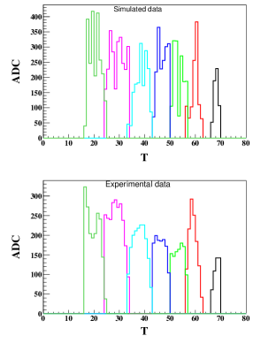
Figure 10: Simulated (upper) and experimental (lower) ADC and T distributions of a single track. The different colors indicate the signals from different pads, the same color in the top and bottom figure indicate that the signal was registered on the same pad.

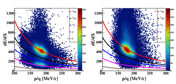
Figure 11: $\small{\frac{dE}{dX}}$ vs. $p/q$ distributions for the left (on the left) and for the right (on the right) half of the RTPC after gain calibration. The lines are theoretical expectations from the Bethe-Bloch formula for ⁴He (red), ³He (black), ³H (blue), ²H (pink) and protons (gray).

5 Track Reconstruction

5.1 Noise Rejection

Two independent noise signatures were identified in the raw data and removed in software prior to track reconstruction. Both are transient and isolated to a subset of the readout channels.

The first is an oscillatory noise located early in the readout time window, shown in the top panel of Figure 12 for a particularly noisy channel. Its amplitude is similar to those of real tracks. About 18% of the readout channels exhibit large contributions from this noise. Due to its unique time-energy correlation, we use a pattern recognition algorithm and discard the hits coming from the channels that display this behavior on an event by event basis. The result of the procedure is illustrated in the bottom panel of Figure 12.

The second noise signature was a coherent noise affecting about 25% of the pre-amplifiers boards, when simultaneous hits in most of the 16 channels of the board were recorded. An event-based technique to identify and remove this noise was developed based on counting simultaneous hits in each pre-amplifier group, and, if sufficiently large, perform a dynamic pedestal subtraction based on the average ADC of neighboring channels within this group.

The sources of these effects were not determined, but rejection techniques allowed to reconstruct 10% more good tracks and recover 70 channels that were previously ignored due to excessive noise levels.

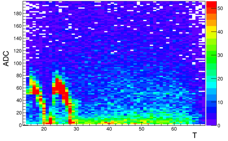
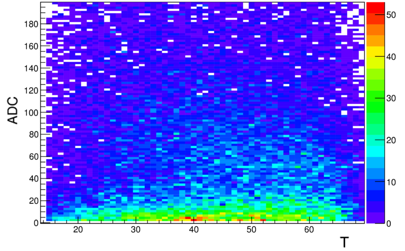
Figure 12: The ADC vs. T spectrum for an example noisy channel before (top) and after (bottom) noise rejection algorithms. Only hits associated with tracks are included, and the selection of events and tracks is the same in both plots.

5.2 Track Fitting

The tracking starts with reconstructing the spacial origin of the hits using the extracted drift speed and drift path parameters. For each registered hit, we calculate the position of emission from the signal time and the pad position. Then, chains of hits are created. The maximum distance between two close adjacent hits has to be less than 10.5 mm to chain them, which roughly corresponds to neighbors and next to neighbors. We fit the chains with a helix if they have a minimum of 10 hits. We then eliminate from the chain the hits that are 5 mm or farther from the fit, as they are not likely part of the same track. This new reduced chain is used for a second and final helix fit.

For energy deposition, the mean $\frac{dE}{dx}$ is calculated as

$$\left\langle\frac{dE}{dX}\right\rangle=\frac{\sum\limits_{i}\frac{ADC_{i}}{G_{i}}}{L},$$ (1)

where the sum runs over all the hits of the track, $G_{i}$ is the gain of the associated pad, and $L$ is the visible track length in the active drift volume.

5.3 Energy Loss Corrections

Energy loss between the target and drift region was significant in the RTPC and necessitated a correction for optimal momentum reconstruction at the primary interaction vertex. The dominant loss was in the 27 µm thick Kapton target wall, with significant contributions also from the pressurized target gas and the foils before reaching the drift region. Corrections were developed based on GEANT4 simulations with the full RTPC geometry and parametrized in terms of recoil curvature in the drift region and polar angle, separately for all recoil hypotheses ($p$, $d$, ³H, ³He, ⁴He). At our average coherent ⁴He DVCS kinematics, energy losses were about 5 MeV, while for $e-^{4}$He elastic scattering losses were about 3 MeV, which corresponds to momentum corrections of 25% and 15%, respectively.

6 Performance Studies

The primary data sample used for calibration and performance assessment of the RTPC was elastic scattering with a 1.2 GeV electron beam. The electron momentum and direction is measured with CLAS, which uniquely determines the expected recoiling ⁴He kinematics. Matching requirements between reconstructed and expected $z$-vertex and direction of the RTPC track provides a clean selection of elastically-scattered ⁴He, shown in Figure 13.

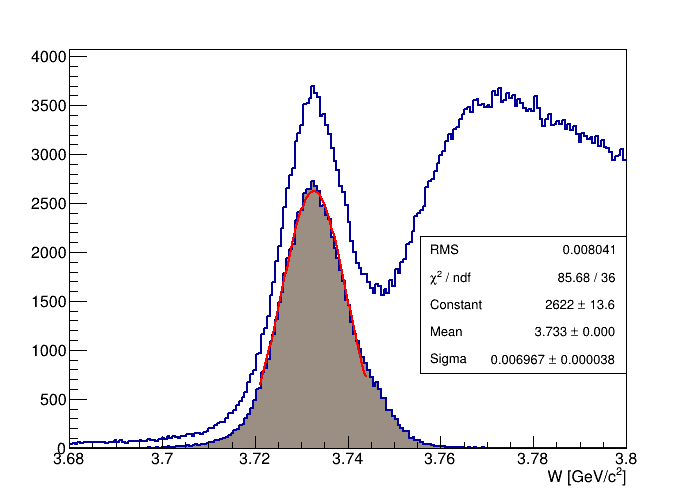
Figure 13: The recoil mass, $W$, distribution calculated from electron kinematics before (“inclusive”) and after (“exclusive”) requiring a matching track in the RTPC.

6.1 Resolution

Elastic scattering was used to estimate the tracking resolution of the RTPC based on the residual between the expected and measured ⁴He tracks. The RTPC resolutions, after removing contributions from the electron, are shown in Table  1, and are very similar for the two halves of the RTPC. Note that the $\theta$- and $z$-resolutions are highly correlated.

	$\sigma_{z}$	$\sigma_{\theta}$	$\sigma_{\phi}$	$\sigma_{p}/p$
Left	5.3 mm	3.8∘	1.9∘	9$\%$
Right	6.5 mm	4.0∘	1.9∘	8$\%$

Table 1: The resolutions of the two modules of the RTPC for $z$-vertex, polar and azimuthal angles, and momentum.

6.2 Efficiency

We measured the efficiency of the RTPC using elastic scattering on ⁴He by comparing the inclusive yield, based only on electron detection, to the exclusive elastic yield, where the Helium recoil is also detected (see Figure 13). We present in Figure 14 the results for the two halves of the detector. We observe that the left and the right modules have similar efficiencies except near the upstream target window. This difference is due to the large number of dead channels concentrated in this part of the left half of the detector

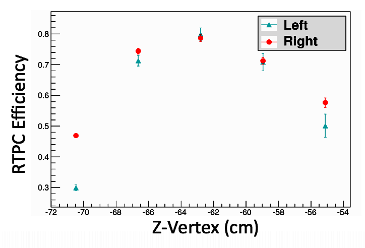
Figure 14: The RTPC ⁴He detection efficiency as a function of the longitudinal position along the detector.

7 Conclusion

We reported on the construction, operation and calibration of a small RTPC designed to measure ⁴He nuclei in high rate environment. The operation of the detector was successful and allowed to detect Helium nuclei with a 75% efficiency and a readout rate of 3.1 kHz triggered by the detection of high energy electrons and photons in the CLAS spectrometer.

8 Acknowledgments

The authors thank the staff of the Accelerator and Physics Divisions at the Thomas Jefferson National Accelerator Facility who made this work possible. This work was supported in part by the French Centre National de la Recherche Scientifique (CNRS), the Italian Istituto Nazionale di Fisica Nucleare (INFN) and the U.S. Department of Energy. M. Hattawy also acknowledges the support of the Consulat Général de France à Jérusalem. The Southeastern Universities Research Association operates the Thomas Jefferson National Accelerator Facility for the United States Department of Energy under contract DE-AC05-06OR23177. This material is based upon work supported by the U.S. Department of Energy, Office of Science, Office of Nuclear Physics, under contract number DE-AC02-06CH11357.

References

- [1] B. A. Mecking et al. [CLAS Collaboration], The CEBAF Large Acceptance Spectrometer (CLAS), Nucl. Instrum. Meth. A 503, 513 (2003).
- [2] M. D. Mestayer et al., The CLAS drift chamber system, Nucl. Instrum. Meth. A 449, 81 (2000).
- [3] G. Adams et al., The CLAS Cherenkov detector, Nucl. Instrum. Meth. A 465, 414 (2001).
- [4] E. S. Smith et al., The time-of-flight system for CLAS, Nucl. Instrum. Meth. A 432, 265 (1999).
- [5] M. Amarian et al., The CLAS forward electromagnetic calorimeter, Nucl. Instrum. Meth. A 460, 239 (2001).
- [6] F. X. Girod et al. [CLAS Collaboration], Measurement of Deeply virtual Compton scattering beam-spin asymmetries, Phys. Rev. Lett. 100, 162002 (2008).
- [7] Hyon-Suk Jo, Etude de la Diffusion Compton Profondément Virtuelle Sur le Nucléon avec le Détecteur CLAS de Jefferson Lab: Mesure des Sections Efficaces polarisées et non polarisées, IPNO-Thesis (2007).
- [8] G. Asryan et al., Meson spectroscopy in the Coherent Production on 4He with CLAS, Jlab proposal to PAC31 (2007).
- [9] K. Hafidi et al., Deeply virtual Comton scattering off 4He, Jlab proposal to PAC33 (2008).
- [10] H. C. Fenker et al., BoNuS: Development and Use of a Radial TPC using Cylindrical GEMs, Nucl. Instrum. Meth. A 592, 273 (2008).
- [11] F. Sauli, The gas electron multiplier (GEM): Operating principles and applications, Nucl. Instrum. Meth. A 805, 2 (2016).
- [12] S. Bachmann et al., Performance of GEM detectors in high intensity particle beams, Nucl. Instrum. Meth. A 470, 548 (2001).
- [13] S. F. Biagi, Monte Carlo simulation of electron drift and diffusion in counting gases under the influence of electric and magnetic fields, Nucl. Instrum. Meth. A 421, no. 1-2, 234 (1999).
- [14] L. Musa et al., The ALICE TPC front end Electronics, Nuclear Science Symposium Conference Record, 2003 IEEE, 5 3647-3651 Vol.5, Oct (2003).
- [15] R. Esteve Bosch, A. Jimenez de Parga, B. Mota and L. Musa, The ALTRO chip: A 16-channel A/D converter and digital processor for gas detectors, IEEE Trans. Nucl. Sci. 50, 2460 (2003).
- [16] C. G. Gutierrez et al., The ALICE TPC Readout Control Unit, IEEE Nuclear Science Symposium Conference Record, 1, 575
- [17] http://geant4.cern.ch