Linked by dynamics:
wavelet–based mutual information rate as a connectivity measure
and scale-specific networks

Abstract

Experimentally observed networks of interacting dynamical systems are inferred from recorded multivariate time series by evaluating a statistical measure of dependence, usually the cross-correlation coefficient, or mutual information. These measures reflect dependence in static probability distributions, generated by systems’ evolution, rather than coherence of systems’ dynamics. Moreover, these “static” measures of dependence can be biased due to properties of dynamics underlying the analyzed time series. Consequently, properties of local dynamics can be misinterpreted as properties of connectivity or long-range interactions. We propose the mutual information rate as a measure reflecting coherence or synchronization of dynamics of two systems and not suffering by the bias typical for the “static” measures. We demonstrate that a computationally accessible estimation method, derived for Gaussian processes and adapted by using the wavelet transform, can be effective for nonlinear, nonstationary and multiscale processes. The discussed problem and the proposed method are illustrated using numerically generated data of coupled dynamical systems as well as gridded reanalysis data of surface air temperature as the source for the construction of climate networks. In particular, scale-specific climate networks are introduced.

To appear in: Tsonis, A.A. (ed.): Advances in Nonlinear Geosciences, Springer, 2017.

I Introduction

“More is different,” the simple sentence of the most creative Soler (2006) physicist P.W. Anderson Anderson (1972) reflects the complex reality in which the behavior of complex systems, consisting of many interacting elements, cannot be explained by a simple extrapolation of the laws describing the behavior of a few elements. Studying systems of many interacting elements as complex networks Albert and Barabási (2002); Boccaletti et al. (2006); Newman et al. (2006); Havlin et al. (2012) is an intensively developing paradigm in which statistical physics embraced the graph theory. In the graph-theoretical characterization of complex networks, a network is considered as a graph $G=(V,E)$, where $V$ is a set of nodes (or vertices) and $E$ is a set of edges (or links) where each edge represents a connection between two nodes. In the case of weighted graphs a weight $w_{i,j}$ is assigned to each edge $e_{i,j}$, connecting the vertices $v_{i}$ and $v_{j}$, by the weight function $W:E\rightarrow\mathbb{R}$. The graph $G=(V,E)$ is characterized by the adjacency matrix $A$ whose elements $a_{i,j}=w_{i,j}$; and $a_{i,i}=0$ by definition. We will consider undirected graphs, i.e. $a_{i,j}=a_{j,i}$. A special case of graphs are unweighted graphs, also known as binary graphs, since $a_{i,j}$ can attain either the value 1 if $e_{i,j}\in E$, or the value $0$ otherwise.

In this study we will consider networks of interacting, possibly stochastic, dynamical systems. In the network paradigm, each system represents a node of the network. Consider that the interactions among the nodes (dynamical systems) are not known. However, we can observe and record evolution of each dynamical system. A series of measurements done on such a system in consecutive instants of time $t=1,2,\dots$ is usually called a time series $\{x(t)\}$. In order to infer a network from a multivariate time series $\{x_{i}(t)\}$ usually some measure of statistical dependence between components $\{x_{i}(t)\}$ and $\{x_{j}(t)\}$, recorded from the nodes $v_{i}$ and $v_{j}$, respectively, is estimated. This measure, or a transformation thereof, is considered as a weight $w_{i,j}$ assigned to the edge $e_{i,j}$. The networks of this type are known as interaction networks Bialonski et al. (2010) or functional networks. The latter term have been spread from neurophysiology where the statistical association of neural activities in two distinct parts of the brain is called the functional connectivity Friston (1994), as opposed to a structural, anatomical connectivity given by an existence of a physical link Bullmore and Sporns (2009). Neurophysiology is probably the most active and influential scientific field where the functional networks are constructed and studied; making use of a huge amount of multivariate data recording various modes of brain activity Bullmore and Sporns (2009); Achard et al. (2006); Reijneveld et al. (2007). The interaction networks, however, are studied also in different areas such as climatology Tsonis and Roebber (2004); Tsonis et al. (2006); Yamasaki et al. (2008, 2009a); Donges et al. (2009a, b); Steinhaeuser et al. (2012) or economy and finance Schweitzer et al. (2009); Onnela et al. (2004). Since the existence of a link in an interaction network is inferred from an estimate of a statistical dependence measure, the strength and even the existence of a link bear some level of uncertainty. Kramer et al. Kramer et al. (2009) propose a systematic statistical procedure for the inference of functional connectivity networks from multivariate time series yielding as the output both the inferred network and a quantification of uncertainty of the number of edges. Paluš et al. Paluš et al. (2011) present differences in the topology of interaction networks with edges derived either from the largest absolute correlations or from the statistically most significant absolute correlations. Bialonski et al. Bialonski et al. (2010) demonstrate that a spatial sampling can lead to an occurrence of spurious structures in interaction networks constructed from time series sampled in spatially extended systems and propose tailored random networks as a suitable null hypothesis to be tested Bialonski et al. (2011). Hlinka et al. Hlinka et al. (2012) observed that a spurious small-world topology emerged in interaction networks constructed using correlations of time series generated by randomly connected dynamical systems. While Bialonski et al. Bialonski et al. (2010) attribute spurious topologies to sampling problems and finite-precision, finite-length time series, Hlinka et al. Hlinka et al. (2012) see the problem in partial transitivity – an inherent property of the correlation coefficient. Also Zalesky et al. Zalesky et al. (2012) observed that the networks in which connectivity was measured using the correlation coefficient were inherently more clustered than random networks, while partial correlation networks were inherently less clustered than random networks. Therefore, in a similar line with Bialonski et al. Bialonski et al. (2011), also Zalesky et al. Zalesky et al. (2012) propose to use a sort of null networks in order to explicitly normalize for the inherent topological structure found in the correlation networks.

In this study we will focus on the dynamics underlying time series used for the construction of interaction networks. We will demonstrate how “dynamical memory” influences the bias in estimations of “static” dependence measures such as the absolute correlation coefficient or the mutual information. We will propose the mutual information rate as a measure reflecting dependence of dynamics of two systems or processes. We will introduce a computationally accessible algorithm that can be effective for quantification of the coherence or synchronization of nonlinear, nonstationary and multiscale processes and thus can be used for the construction of interaction networks from experimental time series recorded in natural complex systems.

II Dependence

Consider two discrete random variables $X$ and $Y$ with sets of values $\Xi$ and $\Upsilon$, respectively. The probability distribution function (PDF) $p_{X}(x)$ for the variable $X$, for simplicity denoted as $p(x)$, is $p(x)=$ Pr$\{X=x\}$, $x\in\Xi$. The probability distribution function $p(y)$ for the variable $Y$ is defined in the full analogy; and the joint PDF $p(x,y)$ is Pr$\{(X,Y)=(x,y)\}$, $x\in\Xi$, $y\in\Upsilon$. Uncertainty in a random variable, say $X$, is characterized by its entropy

$$H(X)=-\sum_{x\in\Xi}p(x)\log p(x).$$ (1)

The joint entropy $H(X,Y)$ of $X$ and $Y$ is

$$H(X,Y)=-\sum_{x\in\Xi}\sum_{y\in\Upsilon}p(x,y)\log p(x,y).$$ (2)

The two variables $X$ and $Y$ are independent if and only if $p(x,y)=p(x)p(y)$, i.e.

$$\log\frac{p(x,y)}{p(x)p(y)}=0.$$

The average digression from independence, i.e., the averaged value of $\log\frac{p(x,y)}{p(x)p(y)}$ is known as mutual information

$$I(X;Y)=\sum_{x\in\Xi}\sum_{y\in\Upsilon}p(x,y)\log\frac{p(x,y)}{p(x)p(y)}.$$ (3)

The mutual information can be expressed using the entropies (1), (2) as

$$I(X;Y)=H(X)+H(Y)-H(X,Y).$$ (4)

Thus the mutual information $I(X;Y)$ quantifies the decrease of uncertainty in $H(X,Y)$ due to the dependence between $X$ and $Y$, i.e., it measures the average amount of common information, contained in the variables $X$ and $Y$. The mutual information is a measure of general statistical dependence for which the following statements hold:

• $I(X;Y)\geq 0$,

• $I(X;Y)=0$ iff $X$ and $Y$ are independent.

In practice, however, the PDF’s are not known and we only have a set of measurements $\{x_{1},x_{2},\dots,x_{N}\}$ for the variable $X$ and $\{y_{1},y_{2},\dots,y_{N}\}$ for the variable $Y$. Estimation of the entropies (1), (2) and the mutual information (3) can be done using some of suitable estimators, for review see Ref. Hlaváčková-Schindler et al. (2007).

A common measure of linear dependence is the (Pearson’s) correlation coefficient. First, we compute the mean of all measurements $\{x_{1},x_{2},\dots,x_{N}\}$ as

$$\bar{x}=\frac{1}{N}\sum_{i=1}^{N}x_{i}$$

and the variance

$$\sigma^{2}=\frac{1}{N-1}\sum_{i=1}^{N}(x_{i}-\bar{x})^{2}$$

and transform the measurements into a data with a zero mean and a unit variance

$$\widetilde{x_{i}}=\frac{x_{i}-\bar{x}}{\sigma}.$$ (5)

After the same procedure with the measurements of the variable $Y$, the correlation coefficient of $X$ and $Y$ is

$$C(X,Y)=\frac{1}{N}\sum_{i=1}^{N}\widetilde{x}_{i}\widetilde{y}_{i}.$$ (6)

Without loss of generality, in the following we will suppose that considered data or time series have (or have been transformed in order to have) a zero mean and a unit variance.

Suppose that the variables $X$ and $Y$ have a bivariate Gaussian distribution. Then their mutual information $I(X;Y)$ can be expressed using their correlation coefficient $C(X,Y)$ (see, e.g. Ref. Paluš et al. (1993) and references therein)

$$I(X;Y)=-\frac{1}{2}\log\big{(}1-C^{2}(X,Y)\big{)}.$$ (7)

The correlation coefficient (6) and the mutual information (3) are the measures of dependence which reflect the digression of the “static” bivariate distribution $p(x,y)$ from the product $p(x)p(y)$. We use the term “static” in order to stress that both the correlation coefficient (6) and the bivariate PDF $p(x,y)$ which determines the mutual information (3) are given by the set of pairs $\{(x_{1},y_{1}),(x_{2},y_{2}),\dots,(x_{N},y_{N})\}$ irrespectively of the order of the pairs. Any permutation of the pairs $(x_{i},y_{i})$ yields the same result.

III Dynamics

Let us consider $n$ discrete random variables $X_{1},\dots,X_{n}$ with values $(x_{1},\dots,x_{n})\in\Xi_{1}\times\dots\times\Xi_{n}$. The PDF for an individual $X_{i}$ is $p(x_{i})=$ Pr$\{X_{i}=x_{i}\}$, $x_{i}\in\Xi_{i}$, the joint PDF for the $n$ variables $X_{1},\dots,X_{n}$ is $p(x_{1},\dots,x_{n})=$ Pr$\{(X_{1},\dots,X_{n})=(x_{1},\dots,x_{n})\}$. The joint entropy of the $n$ variables $X_{1}$,$\dots$, $X_{n}$ with the joint PDF $p(x_{1},\dots,x_{n})$ is

$$H(X_{1},\dots,X_{n})=$$

$$-\sum_{x_{1}\in\Xi_{1}}\dots\sum_{x_{n}\in\Xi_{n}}p(x_{1},\dots,x_{n})\log p(x_{1},\dots,x_{n}).$$ (8)

A stochastic process $\{X_{i}\}$ is an indexed sequence of random variables $X_{1},\dots,X_{n}$, characterized by the joint PDF $p(x_{1},\dots,x_{n})$. Uncertainty in a variable $X_{i}$ is characterized by its entropy $H(X_{i})$. The rate at which a stochastic process “produces” uncertainty is measured by its entropy rate

$$h=\lim_{n\rightarrow\infty}\frac{1}{n}H(X_{1},\dots,X_{n}).$$ (9)

In practice we will deal with a time series $\{x(t)\}$, $t=1,2,\dots,N$. While considering measurements $\{x_{1},x_{2},\dots,x_{N}\}$ of a random variable $X$, its values $x_{i}$ are typically considered mutually independent, i.e., obtained by independent, random draws from a PDF $p(x)$. On the other hand, a time series $\{x(t)\}$ reflects a temporal evolution of a process or a system, and typically the values $x(t)$ and $x(t+\tau)$, where $\tau$ is a time lag, are not independent. The level of dependence between $x(t)$ and $x(t+\tau)$ reflects a “dynamical memory” of the temporal evolution of an underlying process or system. The decrease of the dependence between $x(t)$ and $x(t+\tau)$, with increasing $\tau$, i.e., the rate at which a process “forgets” its history depends on complexity of the temporal evolution of a process or a system and we will refer to this complexity as “temporal dynamics,” or shortly as “dynamics.”

Since a time series $\{x(t)\}$ reflects the dynamics of an underlying process or system, a stochastic process $\{X_{i}\}$ characterized by the joint PDF $p(x_{1},x_{2}\dots,x_{n})$ which typically differs from the product $p(x_{1})p(x_{2})\dots p(x_{n})$, is an appropriate theoretical concept for the study of time series. Thus a time series is considered as a realization of a stochastic process $\{X_{i}\}$, and should not be equated with a set of measurements of a single variable $X$ with a PDF $p(x)$. The entropy rate (9) is a useful characterization of the dynamics of a system or a process underlying the time series $\{x(t)\}$. In information theory the entropy rate (9) is considered as a measure of production of information of an information source Cover and Thomas (1991).

Alternatively, a time series $\{x(t)\}$ can be considered as a projection of a trajectory of a dynamical system, evolving in a measurable state space. A. N. Kolmogorov, who introduced the theoretical concept of classification of dynamical systems by information rates, was inspired by information theory and generalized the notion of the entropy of an information source. The Kolmogorov-Sinai entropy (KSE thereafter) or metric entropy Petersen (1989) is a topological invariant, suitable for the classification of dynamical systems or their states, and is related to the sum of the system’s positive Lyapunov exponents Pesin (1977). The concept of entropy rates is common to theories based on philosophically opposite assumptions (randomness vs. determinism) and is ideally applicable for the characterization of complex processes, where possibly deterministic rules are always accompanied by random influences.

As a potentially useful quantitative characterization of the dynamics, the entropy rate has become a target of many numerical algorithms using experimental time series as their input. Particularly intensive development, focused on the estimation of the metric entropy, has started with the advent of the methods for the reconstruction of chaotic dynamics in the 1980’s. Grassberger and Procaccia Grassberger and Procaccia (1983a) used the concept of Rényi entropy Cover and Thomas (1991) to redefine the KSE in the terms of the Rényi entropy of order two and proposed an estimator of the metric entropy $K_{2}$ using their celebrated correlation integral Grassberger and Procaccia (1983b). The method has been extended into numerous version, e.g. by Cohen and Procaccia Cohen and Procaccia (1985). Schouten et al. Schouten et al. (1994) treated the correlation integral as a probability distribution and derived a maximum-likelihood estimator of the KSE. Pawelzik and Schuster Pawelzik and Schuster (1987) consider the full spectrum of generalized metric entropies $K_{q}$. Fraser Fraser (1989) pointed to an interesting relation between an n-dimensional version of the mutual information and the KSE of a dynamical system underlying studied time series. Paluš Paluš (1997a) studied this relation in detail and confirmed its validity by comparing the KSE estimates with the values of the positive Lyapunov exponents of the studied chaotic systems. Reliable KSE estimates, however, require large amounts of data. Therefore Paluš Paluš (1996a) proposed “coarse-grained entropy rates” which relate the KSE to the rate of the decrease of a finite-precision mutual information of a time series and its time-lagged twins. Also bounded by a finite precision and a limited amount of real data, Pincus Pincus (1991) introduced an approximate entropy based on a difference of the correlation integrals.

The entropy rate reflects how quickly a system “forgets” its history. In the case of chaotic dynamical systems the metric entropy is related to a time interval which a dynamical system takes to return to a close vicinity of some of its previous states. Baptista et al. Baptista et al. (2010) propose two formulas to estimate the KSE and its lower bound from the recurrence times of chaotic systems. The recurrence plots Marwan et al. (2007) give a number of useful dynamical quantities including the KSE.

A time series of measurements of a finite precision can be conveniently converted into a sequence of symbols from a finite set of values. Bandt and Pompe Bandt and Pompe (2002) introduced the concept of permutation entropy for symbolic sequences and demonstrate its relations to the KSE. Lesne et al. Lesne et al. (2009) studied entropy rate estimators for short symbolic sequences based on block entropies and Lempel-Ziv complexity Ziv and Lempel (1978). Kennel et al. Kennel et al. (2005) developed an algorithm for estimating the entropy rate of Markov models using weighted context trees. The entropy rates can also be computed using the causal state machine based estimator Crutchfield and Young (1989); Shalizi and Crutchfield (2001); Haslinger et al. (2010).

Let us return from symbolic sequences to continuous stochastic processes. Let a stochastic process $\{X_{i}\}$ is a zero-mean, stationary, Gaussian process with power spectral density $\Phi(\omega)$, where $\omega$ is a normalized frequency. Then its entropy rate $h_{G}$, apart from a constant term, is Pinsker (1964); Paluš (1997b)

$$h_{G}=\frac{1}{2\pi}\int^{2\pi}_{0}\log\Phi(\omega)d\omega.$$ (10)

IV Dynamics and connectivity

In order to understand the notion of temporal dynamics of a process and its characterization using the entropy rate, let us consider the autoregressive process (ARP)

$$x(t)=c\sum_{k=1}^{10}a_{k}x(t-k)+\sigma e(t),$$ (11)

where $a_{k=1,..,10}={0,0,0,0,0,.19,.2,.2,.2,.2}$, $\sigma=0.01$ and $e(t)$ is a Gaussian noise with a zero mean and a unit variance. The parameter $c$ modulates the proportion of the deterministic part of the process which is a function of the history of the process, to the noise part of the process. The greater the coefficient $c$, the stronger the memory, i.e., the dependence between $x(t)$ and $x(t+\tau)$.

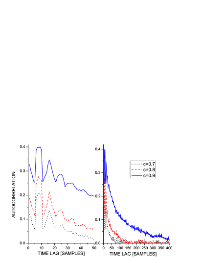
Figure 1: (Color online) Autocorrelation function for the autoregressive process (11) for different values of the coefficient $c$: $c=0.7$ (the dotted black line), $c=0.8$ (the dashed red line), and $c=0.9$ (the solid blue line). Time lags 1–400 samples (right panel), the detail for time lags 1–50 samples (left panel).

This effect is demonstrated in Fig. 1, where the autocorrelation function $C\big{(}x(t),x(t+\tau)\big{)}$ as a function of the time lag $\tau$ is plotted for different values of the coefficient $c$. For $c=0.7$ (the dotted black line) the autocorrelation function (ACF) has the lowest values and vanishes (fluctuates with values close to zero) for time lags around 100 samples; for $c=0.8$ (the dashed red line) the ACF has higher values and vanishes about the time lag equal to 150 samples, while for $c=0.9$ (the solid blue line) the ACF has the largest values and requires more than 400 samples of the time lag to vanish. The ACF reflects the fact that increasing $c$ the dynamical memory of the process (11) is stronger and longer lasting.

Figure 2: (a) Entropy rate $h_{G}$ for the autoregressive process (11) as a function of the parameter $c$. (b) Dependence of the mean absolute cross-correlation between independent realizations of the autoregressive process (11) on the parameter $c$.

How these differences in the dynamical memory, or in the dynamics are reflected in the entropy rate? We generate realizations of the ARP (11) with different $c$ and compute the entropy rates $h_{G}$ according to Eq. (10). Figure 2a presents the entropy rate $h_{G}$ for 100 realizations of the ARP (11) with $c$ increasing from 0.5 to 0.9. The entropy rate of such ARP’s monotonically decreases with increasing $c$. A higher entropy rate means that the process generates uncertainty at a higher rate so that it forgets its history more quickly. Predictability of a process with a higher entropy rate is worse and possible for a shorter prediction horizon than predictability of a process with a lower entropy rate.

Time series $\{x_{i}(t)\}$ recording temporal evolution of different systems or subsystems of a complex system might reflect different dynamics yielding different entropy rates. As we have noted in the Introduction, the connectivity in complex networks constructed from multivariate time series, i.e., the existence and the strength of links between nodes are inferred using dependence measures such as the mutual information (3) and the correlation (6). The absolute value of the latter is typically used, while the mutual information is always non-negative. Applying the definitions (3) and (6) to time series $\{x(t)\}$ and $\{y(t)\}$, they are treated as sets $\{x_{i}\}$ and $\{y_{i}\}$ of measurements of random variables $X$ and $Y$. The computed $C(X,Y)$ or $I(X;Y)$ do not reflect the dynamics of $\{x(t)\}$ and $\{y(t)\}$. Indeed, the pairs $(x(t),y(t))$ would yield the same values of $C(X,Y)$ or $I(X;Y)$ independently of their temporal order. The computed values of $C(X,Y)$ or $I(X;Y)$ are, however, only estimates of the true dependence between processes generating the datasets $\{x(t)\}$ and $\{y(t)\}$. The estimates have some bias, giving a mean digression from the true value, and a variance giving the range of fluctuations of the estimates around their mean value.

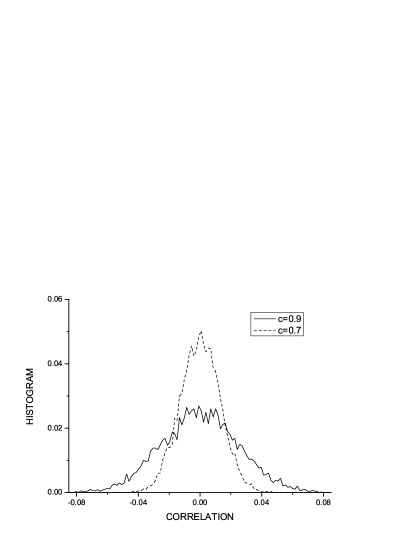
Figure 3: Histograms of cross-correlations between independent realizations of the autoregressive process (11) for two different values of the parameter $c$.

Using the above defined ARP (11) we can study the behavior of the correlation estimates for time series with different dynamics. In particular, we can generate realizations of the ARP (11) with different $c$’s and thus with different entropy rates. Now, let us study the distribution of the cross-correlations between independent realizations of the process (11) for different values of the parameter $c$. For each $c$ we generate 8192 process realizations, each realization consisting of 16,384 samples. Figure 3 presents histograms of cross-correlations between independent realizations of ARP (11) for two different $c$’s. The mean value is always correctly equal to zero, however, the variance increases with increasing $c$, i.e., with decreasing the entropy rate. As a consequence, when considering the absolute correlations, or a non-negative dependence measure such as the mutual information, its mean value has an increasing upward bias with the decreasing entropy rate. This effect is illustrated in Fig. 2b. In this example the bias in the absolute correlations reaches relatively small values 0.01 – 0.02. These values, however, are obtained for time series of 16,384 samples. In Sec. VIII we will show that in real time series of 512 samples the bias can reach such values as 0.4. For even shorter and/or more regular (lower entropy rate) time series the bias can be even higher Paluš (2007).

V Mutual information rate

Instead of treating time series $\{x(t)\}$ and $\{y(t)\}$ as sets $\{x_{i}\}$ and $\{y_{i}\}$ of measurements of random variables $X$ and $Y$, now let us consider the time series $\{x(t)\}$ and $\{y(t)\}$ as realizations of stochastic processes $\{X_{i}\}$ and $\{Y_{i}\}$, characterized by PDF’s $p(x_{1},\dots,x_{n})$ and $p(y_{1},\dots,y_{n})$, respectively. In the analogy of generalization of the entropy (1) to the entropy rate (9) in order to characterize dynamics of a process, now we generalize the mutual information (3) to the mutual information rate (MIR) Cover and Thomas (1991) as

$$i(X_{i};Y_{i})=\lim_{n\rightarrow\infty}\frac{1}{n}I(X_{1},\dots,X_{n};Y_{1},\dots,Y_{n}).$$ (12)

While the mutual information $I(X;Y)$ evaluates the difference between the bivariate PDF $p(x,y)$ and the product of the univariate PDF’s $p(x)p(y)$, the MIR (12) is the limit value of the mutual information $I(X_{1},\dots,X_{n};Y_{1},\dots,Y_{n})$ evaluating the difference between the $2n$-variate PDF $p(x_{1},\dots,x_{n},y_{1},\dots,y_{n})$ and the product of the two $n$-variate PDF’s $p(x_{1},\dots,x_{n})p(y_{1},\dots,y_{n})$. The MIR quantifies the dependence between the sequences of states $X_{1},\dots,X_{n}$ of the process $\{X_{i}\}$ and states $Y_{1},\dots,Y_{n}$ of the process $\{Y_{i}\}$. In the case of dynamical systems the MIR reflects coherent dynamics or a common evolution of two systems whose trajectories are projected onto the time series $\{x(t)\}$ and $\{y(t)\}$.

For pairs of dynamical systems that are either mixing, or exhibit fast decay of correlations, or have sensitivity to initial conditions, Baptista et al. Baptista et al. (2012) have proposed a way how to calculate MIR and its upper and lower bounds in terms of Lyapunov exponents, expansion rates, and capacity dimension. In general, estimators of MIR are well elaborated for symbolic dynamics, extending the estimators of the entropy rates. Shlens et al. Shlens et al. (2007) further develop the estimator of Kennel et al. Kennel et al. (2005) and applied it in order to estimate the information transfer between a stimulus and neural spike trains. Blanc et al. Blanc et al. (2011) extended the entropy rate estimator for symbolic sequences Lesne et al. (2009) and compared several estimators adapted for the estimation of the MIR between coupled dynamical systems in a symbolic representation, including the Lempel-Ziv Ziv and Lempel (1978) and the causal state machine based estimator Crutchfield and Young (1989); Shalizi and Crutchfield (2001); Haslinger et al. (2010).

Considering continuous stochastic processes, for zero-mean, Gaussian stochastic processes $\{X_{i}\}$, $\{Y_{i}\}$, characterized by power spectral densities (PSD) $\Phi_{X}(\omega)$, $\Phi_{Y}(\omega)$ and cross-PSD $\Phi_{X,Y}(\omega)$, the MIR can be expressed (see Ref. Pinsker (1964)) as

$$i_{G}(X_{i};Y_{i})=-\frac{1}{4\pi}\int^{2\pi}_{0}\log(1-|\Gamma_{\small{X,Y}}(\omega)|^{2})d\omega,$$ (13)

using the magnitude-squared coherence

$$|\Gamma_{X,Y}(\omega)|^{2}=\frac{|\Phi_{X,Y}(\omega)|^{2}}{\Phi_{X}(\omega)\Phi_{Y}(\omega)}.$$ (14)

Now we can return to the ARP (11) and use its independent realizations generated with different values of the parameter $c$ and thus characterized by different entropy rates, in order to study the bias of dependence measures in relation to dynamics (entropy rate).

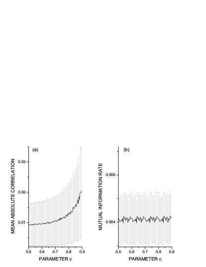
Figure 4: (a) Mean (solid line) and variance (bars $\pm\sigma$ above and below the mean value) of the absolute cross-correlation between independent realizations of the autoregressive process (11) as a function of the parameter $c$. (b) The same as (a) but for the mutual information rate (13). Note that scales in (a) and (b) are different.

In Fig. 4a we study again the absolute cross-correlations of independent realizations the ARP (11) as a function of the parameter $c$. The mean values are the same as in Fig. 2b, however, here we illustrate also the variance as the bars mean$\pm\sigma$. We can see that with increasing $c$ (decreasing the entropy rate) both the mean and variance of the absolute cross-correlations increase. Using the computationally feasible formula (13) for the mutual information rate, in Fig. 4b we present means and variances for the MIR estimates for independent realizations the ARP (11) as a function of the parameter $c$. There is some positive bias, represented by the mean MIR, which is low, randomly fluctuating and independent of the dynamics of the evaluated time series, i.e., independent of the parameter $c$. Also the variances of MIR are independent of $c$, they are practically the same for all values of $c$ – the positions of bars $\pm\sigma$ in Fig. 4b are given by the fluctuations in the mean value. The mutual information rate is a measure of dependence between dynamics of systems or processes, and unlike the static measures, its bias does not depend on the complexity of dynamics.

VI Information rates of Gaussian processes and dynamical systems

The formulas (10) for the entropy rate and (13) for the mutual information rate of Gaussian processes can be efficiently evaluated using the fast Fourier transform (FFT). The question is, however, how applicable are these formulas for real-world time series recorded from complex, possibly nonlinear systems. Using a number of paradigmatic chaotic dynamical systems, Paluš Paluš (1997b) inquired a relation between the Kolmogorov-Sinai entropy of a dynamical system and the entropy rate of a Gaussian process with the same spectrum as the sample spectrum of the time series generated by the dynamical system. An extensive numerical study suggests that such a relation as a nonlinear one-to-one function exists when the Kolmogorov-Sinai entropy varies smoothly with variations of system’s parameters, but is broken near bifurcation points. Although the formula (10) does not give values numerically close to the true values of the Kolmogorov-Sinai entropy of studied dynamical systems, it allows a relative quantification and distinction of different states of nonlinear systems. In a practical application, the formula (10) was used in order to characterize changing complexity of dynamics of neuronal oscillations on route to an epileptic seizure Jiruska et al. (2010). A strongly nonlinear character of the neuronal activity of epileptogenic brain regions has been confirmed, e.g., by Casdagli et al. Casdagli et al. (1996).

Figure 5: Top three panels: bifurcation diagrams of two coupled logistic maps (from the top: $x$, $y$, and $x-y$), for the control parameter value $a=4$, corresponding to fully chaotic maps when uncoupled, as a function of the coupling coefficient $\gamma$. Bottom panel: the mutual information rate (13) between $\{X\}$ and $\{Y\}$, computed using the FFT, as a function of the coupling coefficient $\gamma$.

In order to demonstrate how the formula (13) for the mutual information rate of Gaussian processes reflects changes in the dependence of dynamics of two coupled nonlinear dynamical systems on their route to synchronization we will use two well-know dynamical systems with chaotic behavior. As an example of a discrete-time system let us borrow the symmetrically coupled logistic maps from Blanc et al. Blanc et al. (2011) where the system $\{X\}$ is represented by the time series $\{x_{n}\}$ and the system $\{Y\}$ by the time series $\{y_{n}\}$:

$$\begin{split}x_{n+1}&=&\gamma f_{a}(x_{n})+(1-\gamma)f_{a}(y_{n})\\ y_{n+1}&=&(1-\gamma)f_{a}(x_{n})+\gamma f_{a}(y_{n})\end{split}$$ (15)

where $\gamma$ is the coupling coefficient and varies between 0 and 1. The function $f_{a}(x_{n})\equiv ax_{n}(1-x_{n})$. It is known that, in the uncoupled case, $a=4$ gives a chaotic behavior. The latter is demonstrated in the bifurcation diagrams in Fig. 5 where for small $\gamma$ both the system $\{X\}$ and $\{Y\}$ are chaotic and not synchronized. For $0.13<\gamma<0.2$ a zone of periodic behavior appears, followed by the fully chaotic regime from $\gamma$ approaching $0.2$. The two systems become fully synchronized from $\gamma\approx 0.25$ – in the bifurcation diagram the difference $x-y$ stays on the zero value, i.e., the trajectories of the systems $\{X\}$ and $\{Y\}$ are identical. Then we observe a quasi-symmetry about $\gamma=0.5$, i.e., the synchronized behavior ends for $\gamma>0.75$ and we observe the chaotic, periodic and again chaotic behavior of the unsynchronized systems. This development is reflected in the mutual information rate (13), depicted in the bottom of Fig. 5. With $\gamma$ increasing from zero also the MIR gradually increases, however, it falls down to zero for the interval of periodic dynamics. Thus the MIR is not simply a measure of dependence of dynamics, it rather quantifies an information transfer between systems or processes. In the case of periodic systems with the zero entropy rate (KSE), also the MIR is zero. In the subsequent chaotic regimes the MIR quickly increases with $\gamma$ approaching the synchronization threshold. During the fully synchronized regime the MIR stays on its maximum value. It is interesting to compare Fig. 5 with Fig. 4 in Ref. Blanc et al. (2011) where the authors present results of their four MIR estimators, stating that the Lempel-Ziv estimator Ziv and Lempel (1978) and the causal state machine based estimator Crutchfield and Young (1989); Shalizi and Crutchfield (2001); Haslinger et al. (2010) gave the most faithful results. The latter are qualitatively equivalent to the results obtained using the formula (13) for the MIR of Gaussian processes, estimated using the FFT (the bottom graph of Fig. 5). The qualitative equivalence means that although the values of the MIR estimates are different, the shapes of the MIR dependence on the coupling parameter $\gamma$ are very similar.

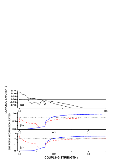
Figure 6: (Color online) (a) Two largest Lyapunov exponents of the drive $\{X\}$ (the constant lines) and the response $\{Y\}$ (the decreasing lines), (b) the entropy rates (10) for the drive $\{X\}$ (the dotted black line) and the response $\{Y\}$ (the dashed red line) and the mutual information rate (13) between $\{X\}$ and $\{Y\}$ (the solid blue line) computed using the FFT; (c) the same as in (b), but computed using the CCWT; for the unidirectionally coupled Rössler systems (VI),(VI), as functions of the coupling strength $\epsilon$. The Lyapunov exponents are measured in nats per a time unit; the entropy and information rates are measured in units of nats per sample.

As an example of a continuous-time system we will consider the unidirectionally coupled Rössler systems, studied also by Paluš and Vejmelka Paluš and Vejmelka (2007), given by the equations

$$\mathaccent 95{x}_{1} = -\omega_{1}x_{2}-x_{3}$$

$$\mathaccent 95{x}_{2} = \omega_{1}x_{1}+a_{1}\;x_{2}$$ (16)

$$\mathaccent 95{x}_{3} = b_{1}+x_{3}(x_{1}-c_{1})$$

for the autonomous system $\{X\}$, and

$$\mathaccent 95{y}_{1} = -\omega_{2}y_{2}-y_{3}+\epsilon(x_{1}-y_{1})$$

$$\mathaccent 95{y}_{2} = \omega_{2}y_{1}+a_{2}\;y_{2}$$ (17)

$$\mathaccent 95{y}_{3} = b_{2}+y_{3}(y_{1}-c_{2})$$

for the response system $\{Y\}$. We will use the parameters $a_{1}=a_{2}=0.15$, $b_{1}=b_{2}=0.2$, $c_{1}=c_{2}=10.0$, and frequencies $\omega_{1}=1.015$ and $\omega_{2}=0.985$, i.e., the two systems are similar, but not identical.

Figure 6a presents four Lyapunov exponents (LE) of the coupled systems (the two negative LE’s are not shown) as functions of the coupling strength $\epsilon$. One positive and one zero LE of the driving system $\{X\}$ are constant, while the LE’s of the driven system $\{Y\}$ which are positive and zero without a coupling or with a weak coupling decrease with increasing $\epsilon$. The two systems can enter a synchronized regime when the originally positive LE of the response system becomes negative. After a transient negativity and a return to zero, the originally positive LE of the driven system $\{Y\}$ becomes decreasing and negative for $\epsilon>0.15$ (Fig. 6a). The mutual information rate (13) between $\{X\}$ and $\{Y\}$ computed using the FFT (the solid blue line in Fig. 6b) gradually increases with the increasing coupling strength $0<\epsilon<0.15$, however, shows a steep increase at or after the synchronization threshold at $\epsilon\approx 0.15$. Then it again increases slowly to its asymptotic value in the synchronized state. At the coupling strength $\epsilon\approx 0.15$ also the entropy rate (10) of the driven system $\{Y\}$ (the dashed red line in Fig. 6b) steeply increases and then continues in a gradual increase and asymptotically approaches the entropy rate (10) of the autonomous system $\{X\}$ (the dotted black line in Fig. 6b). Due to this behavior Paluš et al. Paluš et al. (2001) described the route to synchronization as an adjustment of information rates. It is important that even the mutual information rate (13) of Gaussian processes, computed using the FFT of time series generated by the studied systems, reflects both the gradual increase of coupling as well as the sudden transient into synchronization.

VII MIR and networks of dynamical systems

In Sec. V we have introduced the mutual information rate as a quantity measuring the dependence between dynamics of two systems or processes. Unlike the static measures such as the correlation coefficient or the mutual information of random variables, the estimates of the MIR do not suffer by a bias dependent on the character of dynamics underlying analyzed time series. Blanc et al. Blanc et al. (2011) also show that the MIR is independent of time lag between time evolutions of studied systems. Together with Blanc et al. Blanc et al. (2011) and Baptista et al. Baptista et al. (2012) we propose the MIR as an association measure suitable for inferring interaction networks from multivariate time series generated by coupled dynamical systems. Specifically in this paper we propose to use the formula (13) for the mutual information rate of Gaussian processes. Although Gaussian processes are inherently linear, in Sec. VI we have demonstrated that the MIR (13) computed using the FFT of time series generated by the studied nonlinear dynamical system was able to distinguish not only synchronized from unsynchronized states, but also different levels of dependence between dynamics of the studied systems due to different strengths of their coupling. These observations, however, cannot assure a general applicability of the MIR (13) for natural nonlinear systems. Before constructing networks from experimental multivariate time series it is necessary to test for a presence of nonlinearity in studied time series and assess its actual effect on the inference and quantification of dependence relations present in the data. It is not surprising that such studies have been done in the same areas where the research based on the complex networks paradigm is very active.

Functional brain networks are frequently constructed using time series from sequences of functional magnetic resonance imaging (fMRI) Bullmore and Sporns (2009); Achard et al. (2006). Hlinka et al. Hlinka et al. (2011) demonstrate that the linear correlation coefficient is a sufficient measure of functional connectivity in resting-state fMRI data. Potential new information brought by nonlinear measures such as the mutual information is relatively minor and negligible in comparison with natural intra- and inter-subject variability. Hartman et al. Hartman et al. (2011) confirm this finding in specific computations of graph-theoretical measures from fMRI brain networks. Also spatio-temporal dependence structures in electrophysiological data such as the electroencephalogram (EEG) are characterized within the complex networks paradigm Bullmore and Sporns (2009); Reijneveld et al. (2007). Nonlinear character of the EEG in epilepsy is known Casdagli et al. (1996), some level of nonlinearity can be detected also in normal human EEG recordings Paluš (1996b). Distinction of different physiological and/or pathological brain states observed using nonlinear measures can successfully be reproduced by a proper application od standard tools derived from the theory of linear stochastic processes Theiler and Rapp (1996). While the latter findings characterized single-channel EEG signals, the character of dependence between EEG signals from different parts of the scalp are relevant for the construction of the EEG brain networks. Nonlinear measures have been applied in order to distinguish different consciousness states using so-called multichannel attractor embedding Matousek et al. (1995). Changes in dependence structures in multichannel EEG data which have been described by a nonlinear measure such as the correlation dimension from the multichannel embedding Matousek et al. (1995), however, can be equivalently captured by a linear measure extracted from a correlation matrix Paluš et al. (1992).

Using an equivalent approach, climate networks Tsonis and Roebber (2004); Tsonis et al. (2006); Yamasaki et al. (2008, 2009a); Donges et al. (2009a, b); Steinhaeuser et al. (2012) are constructed using multivariate time series of long-term records of meteorological variables such as the air temperature or pressure. Already in the 1980’s a number of researches attempted to infer nonlinear dynamical mechanisms from meteorological data and claimed detections of a weather or climate attractor of a low dimension Nicolis and Nicolis (1984); Fraedrich (1986); Tsonis and Elsner (1988). Other authors pointed to a limited reliability of chaos-identification algorithms and considered the observed low-dimensional weather/climate attractors as spurious Grassberger (1986); Lorenz (1991). Paluš & Novotná Paluš and Novotná (1994) even found the air temperature data well-explained by a linear stochastic process, when the dependence between a temperature time series $\{x(t)\}$ and its lagged twin $\{x(t+\tau)\}$ was considered. Hlinka et al. Hlinka et al. (2013a) extended the later result to the dependence between the monthly time series of the gridded whole-Earth air temperature reanalysis data. These results do not mean that the dynamics underlying records of meteorological data is linear. For instance, a search for repetitive patterns on specific temporal scales in the air temperature and other meteorological data has led to an identification of oscillatory phenomena possibly possessing a nonlinear origin and exhibiting phase synchronization between oscillatory modes extracted either from different types of climate-related data or data recorded at different locations on the Earth Paluš and Novotná (2004, 2006, 2009); Feliks et al. (2010); Paluš and Novotná (2011). The studies of Hlinka et al. Hlinka et al. (2013a, b) merely state that for inferring general dependence and causal relations, the approaches derived for Gaussian processes perform very well and nonlinear approaches do not bring substantial new information.

These arguments and the fact that the mutual information rate estimator, computed using the FFT and the formula (13) for the MIR of Gaussian processes is computationally less demanding that estimators for general nonlinear processes, form the basis for our recommendation of the MIR (13) as a measure suitable for inference of networks from experimental multivariate time series recorded from complex systems of various origins. There is still a serious demand for the amount and stationary character of the analyzed data, since the computation of the magnitude-squared coherence (14) is based on dividing the time series into a number of segments over which the complex cross-spectrum (the numerator in the Eq. (14) right-hand side) is averaged. In many cases time series from natural complex systems are relatively short and nonstationary. Nonstationarity in the sense of changing relationships between time series with time leads to changes in the strength and even the existence of links in interaction networks during some time intervals. The complex network paradigm copes with this phenomenon using the concept of temporal networks Holme and Saramäki (2012) or evolving networks. The latter approach assumes approximate step-wise stationarity of the analyzed time series and a standard “static” network is inferred in a relatively short time window which is “sliding” over the whole time interval spanned by the available experimental time series. The time evolution of graph-theoretical characteristics is then studied with respect to a time evolution and/or an occurrence of marked events in the studied complex system. This approach has been successfully applied in the EEG brain networks Kuhnert et al. (2010); Bialonski and Lehnertz (2013); Lehnertz et al. (2014), as well as in the climate networks Radebach et al. (2013). An alternative approach, applied in the field of climate networks, is “picking-up” a number of unequal-length subsets of the whole time series, tight to an occurrence of some phenomenon (e.g. El Niño) and performing the summation in the formula (6) for the correlation coefficient only using the selected subsets of the data Tsonis and Swanson (2008). Neither the latter approach, nor the evolving network strategy can be applied when using the standard FFT-based evaluation of the MIR (13).

In order to cope with nonstationarity we propose to use a wavelet transform instead of the Fourier transform. In particular, the complex continuous wavelet transform (CCWT) is applied in order to convert a time series $x(t)$ into a set of complex wavelet coefficients $W(t,f)$:

$$W(t,f)=\int_{-\infty}^{\infty}\psi(t^{\prime})x(t-t^{\prime})dt^{\prime}$$ (18)

using the complex Morlet wavelet Torrence and Compo (1998):

$$\psi(t)=\frac{1}{\sqrt{2\pi\sigma_{t}^{2}}}\exp(-\frac{t^{2}}{2\sigma_{t}^{2}})\exp(2\pi if_{0}),$$ (19)

where $\sigma_{t}$ is the bandwidth parameter, and $f_{0}$ is the central frequency of the wavelet. $\sigma_{t}$ determines the rate of the decay of the Gauss function, its reciprocal value $\sigma_{f}=1/\pi\sigma_{t}$ determines the spectral bandwidth. In order to keep the wavelet representation close to the original MIR (13) evaluation based on the FFT, we use a set of equidistantly spaced central wavelet frequencies in the relevant frequency range given by the time series length and its sampling frequency, instead of the power-law pyramidal scheme, usually used in the wavelet context. Then the product of the complex wavelet coefficients $W_{X}(t,f)W_{Y}^{*}(t,f)$, as well as the norms $|W_{X}(t,f)|$, $|W_{Y}(t,f)|$ are averaged over time $t$. Finally, the wavelet magnitude-squared coherence

$$|\Gamma_{X,Y}^{W}(f)|^{2}=\frac{|W_{X,Y}(f)|^{2}}{|W_{X}(f)||W_{Y}(f)|}$$ (20)

is used in the summation over the set of the central wavelet frequencies according to Eq. (13). Here $W_{X,Y}(f)$, $|W_{X}(f)|$, and $|W_{Y}(f)|$ stand for the time averages of $W_{X}(t,f)W_{Y}^{*}(t,f)$, $|W_{X}(t,f)|$, and $|W_{Y}(t,f)|$, respectively.

Let us return to the unidirectionally coupled Rössler systems (VI), (VI). Using the wavelet representation we can recompute both the mutual information rate (13) and the entropy rate (10) as functions of the coupling strength $\epsilon$ (Fig. 6c) . While the CCWT-based estimators give different values than the FFT-based estimators, they agree in the qualitative sense that the curves of the $\epsilon$-dependence of the MIR in Figs. 6b and 6c (solid/blue curves) are the same. The two estimators also give a good agreement in the $\epsilon$-dependence of the entropy rates (dashed/red curves in Figs. 6b and 6c), there is just a small difference in the entropy rates of the driven system for very small values of $\epsilon$.

It is important that the wavelet-based estimator of the MIR (13) gives a relative distinction of coupling regimes with different coupling strengths. This is a property which we expect from an association measure suitable for the inference of interaction networks from multivariate time series. It will assign proper weights to network edges, an edge of two more strongly coupled nodes (dynamical systems) will obtain a greater weight than edges connecting nodes with a weaker coupling. For the construction of the binary networks, a greater value of MIR for strongly coupled nodes assure an existence of an edge by exceeding a chosen threshold or a critical value given by a statistical test. For establishing statistically significant links we propose to use the surrogate data strategy as described in Refs. Paluš and Vejmelka (2007); Paluš (2007). The temporal averaging of the product of the complex wavelet coefficients $W_{X}(t,f)W_{Y}^{*}(t,f)$ might evoke a temptation to randomize the phases $\varphi$ of the complex wavelet coefficients $W(t,f)\equiv A(t,f)\exp\big{(}i\varphi(t,f)\big{)}$. Generating the FFT-based surrogate data Theiler et al. (1992), the set of the original phases of the Fourier coefficient is substituted by a set of independent, identically distributed (IID) phases randomly sampled from a uniform distribution on the interval $(0,2\pi)$. However, the phase differences of the wavelet coefficients of two signals are not IID, even if the underlying processes are independent. Using random IID phases in the summation of $W_{X}(t,f)W_{Y}^{*}(t,f)$ would underestimate the critical values in the test for independence and false edges would be inferred. The character of the (long-range) dependence of the phase differences in $W_{X}(t,f)W_{Y}^{*}(t,f)$ of independent processes depends on the central wavelet frequency. Therefore, it is more convenient to generate surrogate data and estimate the MIR from them as in the usual surrogate data test strategy Paluš and Vejmelka (2007); Paluš (2007).

Unlike in the FFT-based MIR estimation, we apply the CCWT on the whole time interval of available data. Then we either average the product of the complex wavelet coefficients $W_{X}(t,f)W_{Y}^{*}(t,f)$, as well as the norms $|W_{X}(t,f)|$, $|W_{Y}(t,f)|$, over the whole time interval or apply the sliding-window strategy of the evolving networks Radebach et al. (2013) or the strategy of Tsonis and Swanson Tsonis and Swanson (2008) of the averaging over time intervals selected according to an occurrence of a specific phenomenon. Using the strategies that cope with nonstationarity, however, one should consider a smoothing effect of the wavelet coefficients for low frequencies (large time scales). Since time series from natural complex systems frequently reflect processes with a $1/f$ spectrum, the wavelet coefficients for low frequencies have much greater weights than the coefficients for high frequencies and effects of short-living phenomena can be masked in the resulted MIR estimates. Therefore we recommend to limit the final summation in the MIR formula (13) to higher frequencies or shorter time scales in which the effect of short-living phenomena is not attenuated. The latter idea can be generalized and even for stationary time series one can restrict the MIR evaluation to a specific range of time scales, i.e. to a specific spectral band. Then a scale-specific or frequency-specific connectivity is evaluated and scale-specific or frequency-specific interaction networks can be studied.

Until now we have considered the MIR $i(X_{i};Y_{i})$ of two stochastic processes $\{X_{i}\}$, $\{Y_{i}\}$. Constructing a network of $n$ nodes, i.e., $n$ dynamical systems, we will consider $n$ time series as realizations of $n$ stochastic processes $\{X^{k}_{i}\}$, $k=1,\dots,n$. (For simplicity we consider $n$ univariate time series/stochastic processes, an equivalent of a multivariate stochastic process with $n$ components. The considerations here can be generalized to $n$ multivariate stochastic processes with various numbers $n_{i}$ of components.) Then we can evaluate the standard bivariate MIR $i(X^{k}_{i};X^{l}_{i})$ for each pair of components. In order to distinguish direct from indirect interactions we can also consider conditional (partial) MIR $i(X^{k}_{i};X^{l}_{i}|X^{j}_{i};j=1,\dots,n,j\neq k,j\neq l)$ which quantifies the “net” dependence between the two processes without an influence of the remaining $n-2$ processes.

For the evaluation of the conditional MIR, in the framework of Gaussian processes, we will follow the work of Schelter et al. Schelter et al. (2006) who extended the notion of partial correlations to the partial mean phase coherence.

For each pair of processes $\{X^{k}_{i}\}$, $\{X^{l}_{i}\}$ and each central wavelet frequency $f\in\{f_{1},f_{2},\dots,f_{N_{f}}\}$ we evaluate the time-averaged complex wavelet coherence

$$\Gamma_{k,l}^{W}(f)=\frac{W_{k,l}(f)}{\sqrt{|W_{k}(f)||W_{l}(f)|}}.$$ (21)

Thus for each $f$ we obtain a complex $n\times n$ matrix $\Gamma^{W}(f)$. This complex matrix is inverted, $\Omega(f)=(\Gamma^{W}(f))^{-1}$. Using the entries of the inverted complex matrix $\Omega(f)$ we evaluate the conditional wavelet coherence as

$$\Upsilon_{k,l}(f)=\frac{\Omega_{k,l}(f)}{\sqrt{|\Omega_{k,k}(f)||\Omega_{l,l}(f)|}}.$$ (22)

Finally, the magnitude-squared conditional wavelet coherence is used in the summation according to Eq. (13) in order to obtain the conditional MIR

$$i_{G}(X^{k}_{i};X^{l}_{i}|X^{j}_{i};j=1,\dots,n,j\neq k,j\neq l)=$$

$$-\frac{1}{2N_{f}}\sum_{f=f_{1}}^{f_{N_{f}}}\log(1-|\Upsilon_{{k,l}}(f)|^{2}).$$ (23)

VIII Climate networks

Understanding the complex dynamics of the Earth atmosphere and climate is a great scientific challenge with a potentially high societal impact. In their seminal paper, Tsonis and Roebber Tsonis and Roebber (2004) have proposed to study the climate system as a complex network. Since then the field of climate networks is rapidly developing and expanding in the scope of methodology as well as applications. The spatio-temporal dynamics of the atmosphere is captured by multivariate time series of long-term recordings of meteorological variables. Typically, such instrumental data are preprocessed and interpolated in order to assign a time series of a variable to each node of a regular angular grid covering the Earth surface, as well as slices of the atmosphere at various altitude or air pressure levels. Such gridded time series of meteorological variables, available due to, e.g., the NCEP/NCAR reanalysis project Kalnay et al. (1996) are usually, although not exclusively, used for the construction of climate networks. Monthly Tsonis and Swanson (2008); Donges et al. (2009a) or daily Yamasaki et al. (2008); Gozolchiani et al. (2008) surface air temperature data are frequently used, however, equipotential heights Tsonis et al. (2008); Donges et al. (2011), sea surface temperature, humidity, precipitation and related data Steinhaeuser et al. (2012); Malik et al. (2012) and other meteorological data are also analysed. Individual grid-points, characterized by time series of a chosen meteorological variable, are considered as nodes (vertices) of a climate network, while links (edges) are inferred from some, mostly statistical association between the time series related to the two nodes at the edge’s end-points. The most common association measure is the Pearson’s correlation coefficient Tsonis and Roebber (2004); Tsonis and Swanson (2008), however, also the Spearman’s rank correlation coefficient is used Carpi et al. (2012), and more general, nonlinear measures are tested, e.g., the bivariate mutual information Donges et al. (2009a, b), and the mutual information of ordinal time series Barreiro et al. (2011); Deza et al. (2013) or measures from the phase synchronization analysis Yamasaki et al. (2009b) and the event synchronization analysis Malik et al. (2012).

In the following study we use monthly mean values of the near-Surface Air Temperature (SAT) from the NCEP/NCAR reanalysis (Kalnay et al., 1996). We include the data up to the latitudes 87.5^∘ in the grid of 2.5^∘x2.5^∘ which leads to 10,224 grid points or network nodes. The temporal interval of 624 months starting in January 1958 and ending in December 2009 is used for the inference of the network using the correlation coefficient and the CCWT-based MIR estimator. For the FFT-based estimator the temporal interval is extended backward by 16 months (starting in September 1956) in order to have 5 segments of 128 monthly samples.

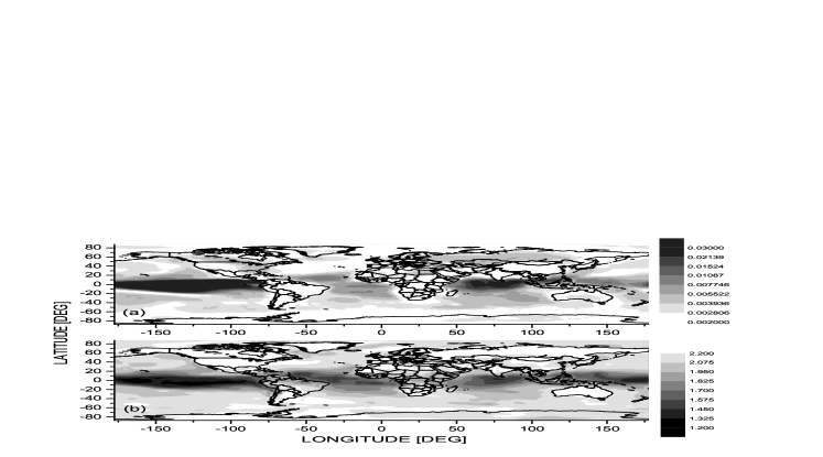
Figure 7: (a) Area weighted connectivity for the SATA climate network with the density $\varrho=0.005$ obtained by the uniform thresholding of the absolute correlations. (b) Complexity of each node SATA time series measured by the Gaussian process entropy rate $h_{G}$. Note the reversed grey scales, the black color corresponds to the largest AWC in (a), while in (b) it corresponds to the lowest entropy rates.

In order to avoid trivial correlations due to seasonal temperature variability, the annual cycle has been removed from each SAT time series. The SAT anomalies (SATA thereafter) have been computed by subtracting the averages for each month from related samples, e.g., the average January temperature was subtracted from all January samples, etc.

As the first step of the network analysis we compute the correlation coefficients $c_{i,j}$ for each pair of nodes $i,j=1,\dots,N_{N}=10224$. We use the matrix of the absolute correlations $C_{i,j}=|c_{i,j}|$ in order to obtain the adjacency matrix $A_{i,j}$ of the binary network, defined as: $A_{i,j}=1$ iff $C_{i,j}>c_{T}$, otherwise $A_{i,j}=0$. $A_{i,i}=0$ by definition. The total number of existing edges divided by the number of all possible edges in known as the network density (or edge density) $\varrho$. Following Donges et al. Donges et al. (2009a, b) we choose the threshold $c_{T}$ such that the resulting network density is $\varrho=0.005$.

The basic characterization of connectivity of a node $i$ is its degree, or degree centrality $k_{i}$

$$k_{i}=\sum_{j=1}^{N_{N}}A_{i,j},$$ (24)

giving the number of nodes to which the node $i$ is connected. Since the reanalysis data are defined on a grid which is regular in the angular coordinates, the geographic distances of the grid points depend on the latitude $\lambda_{i}$. In order to correct for this dependence, for the climate networks defined on the regular angular grid the area weighted connectivity Tsonis et al. (2006) is defined as

$$AWC_{i}=\frac{\sum_{j=1}^{N_{N}}A_{i,j}\cos(\lambda_{j})}{\sum_{j=1}^{N_{N}}\cos(\lambda_{j})}.$$ (25)

The AWC can be interpreted as the fraction of the Earth’s surface area a vertex is connected to.

The AWC computed for each node of the SATA network based on the absolute correlations with $\varrho=0.005$ (AC-network in the following) is mapped in Fig. 7a. According to this analysis the most connected nodes (“hubs”) of the climate network lie in the tropical areas of the Pacific and Indian Oceans. The hub in the tropical Pacific include so-called El Niño areas. The El Niño/Southern Oscillation (ENSO) is a dominant mode of the global atmospheric circulation variability which quasiperiodically causes shift in winds and ocean currents centered in the Tropical Pacific region and is linked to anomalous weather/climate patterns worldwide Sarachik and Cane (2010). The global influence of the El Niño phenomenon is used to explain the observation that the El Niño area constitutes the principal hub of the climate network.

Figure 8: Histograms of cross-correlations of independent FT (solid lines) and amplitude-adjusted FT (dotted lines) surrogate data for the SATA of a pair of nodes from the low entropy rate area (the thin lines, the nodes with the latitude 0^∘, the longitude 90^∘W and 10^∘S, 120^∘W) and a pair from the high entropy rate area (the thick lines, the nodes 60^∘N, 25^∘E and 60^∘N, 75^∘E).

Let us characterize the dynamics of the SATA time series using the entropy rate (10). The FFT-based estimator assign an entropy rate value to each grid-point, i.e. to each node of the network, so they can be mapped in the same way as the AWC. The entropy rate map is presented in Fig. 7b. The correspondence between the lowest entropy rates and the highest AWC of the AC-network is indisputable. In order to assess a bias in the correlation estimator we need time series which are independent, but have the same dynamics (the same entropy rate) as the original SATA time series. Such time series can be generated using the FFT-based surrogate data algorithm Theiler et al. (1992); Paluš (2007). The fast Fourier transform is applied to a time series, the magnitudes of the complex Fourier coefficients are preserved, but their phases are randomized. Using different sets of random phases the inverse FFT generates a number of independent realizations of a Gaussian process with the same spectrum (and thus with the same entropy rate (10)) as that of the original time series. A potential digression from the Gaussian distribution is solved by a histogram transformation known as the amplitude adjustment. We use both the FT surrogate data and the amplitude-adjusted FT (AAFT) surrogate data, however, they give equivalent results. Generating a large number of realizations of the FT (AAFT) surrogate data for the SATA time series we can estimate distributions of the correlations of independent surrogates of the SATA series from various grid-points. Figure 8 compares such histogram for SATA-surrogates for a pair of grid-points from a low entropy rate area (the El Niño area) and from a high entropy rate area (an Euro-Asian area on 60^∘N). While in the Northern hemisphere high entropy rate area the correlation bias (the cross-correlation of realizations of independent processes) scarcely reaches over $\pm 0.1$, in the tropical Pacific areas the cross-correlation bias can reach values close to $\pm 0.4$.

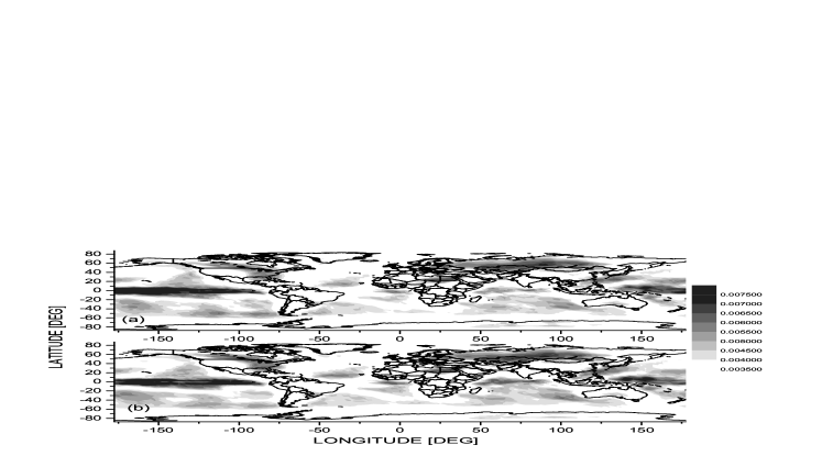
Figure 9: (a) Area weighted connectivity for the SATA climate network with the density $\varrho=0.005$ obtained by the uniform thresholding of the mutual information rate (13) estimated using the Fourier transform (a) and the continuous complex wavelet transform (b). Note that the scale is different from that in Fig. 7a.

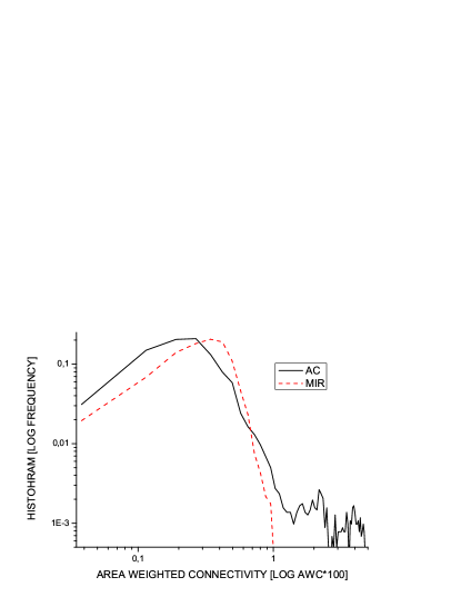
Figure 10: (Color online) Histograms (64 bins) of the area weighted connectivity (AWC*100) for the SATA climate network with the density $\varrho=0.005$ obtained by the uniform thresholding of the absolute correlations (solid black line), and of the mutual information rate (13) (dashed red line).

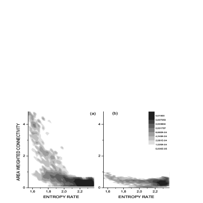
Figure 11: (a) Grey-coded bivariate histograms (32x32 bins) reflecting the joint probability distribution of the SATA entropy rate (10), cf. Fig. 7b, and the area weighted connectivity (AWC*100) for the SATA climate network with the density $\varrho=0.005$ obtained by the uniform thresholding of the absolute correlations, cf. Fig. 7a. (b) The same as in (a), but considering the area weighted connectivity for the SATA climate network with the density $\varrho=0.005$ obtained by the uniform thresholding of the mutual information rate (13), cf. Fig. 9b.

As an alternative we construct a climate network using the MIR (13) and again we threshold the MIR values in order to obtain the network density $\varrho=0.005$. The area weighted connectivity for the MIR-networks is mapped in Fig. 9, where we can compare the results for both the FFT- and CCWT-based estimators. The results are quite similar. A few small differences can be caused by the fact that the FFT-based estimator used segments of 128 samples and thus cannot include the connectivity on large time scales as the CCWT estimator which utilizes 624 samples in one whole segment. The differences between the MIR-network (Fig. 9) and the AC-network (Fig. 7a) are much larger and more important. In the comparison with the AC-network, the very connected hub in the Indian Ocean almost disappears in the MIR network. The hub in the El Niño area survives, however, it is weaker and confined to a smaller area. The connectivity in the continental areas of the Northern hemisphere increases in the MIR-network. This comparison, however, cannot give an answer which network representation is closer to the physical reality.

In the analogy with degree distributions, studied in the complex network theory, in Fig. 10 we present histograms estimating the distributions of the area weighted connectivity. The AWC distribution for the AC-network (the solid black line) shows a heavy irregular tail of extreme AWC values, while the AWC distribution for the MIR-network (the dashed red line) shows a distribution bounded by a fast probability decay for large AWC values, well captured by a Poisson distribution. Scholz Scholz (2010) obtained such distributions using a node-similarity network model. Each node has a set of features, quantified as coordinates in an Euclidean space. Based on a random data set, two nodes are defined as connected (similar) when their Euclidean distance is below a certain threshold. Using a small threshold only very similar (close) nodes are connected. This represents a sparsely connected network showing typically scale-free power-law like distributions. Increasing the threshold, more densely connected networks are modelled with node degree distributions very similar to that of the MIR-network (the dashed red line in Fig. 10).

Figure 12: (a) Area weighted connectivity for the scale-specific SATA climate network with the density $\varrho=0.005$ obtained by the uniform thresholding of the mutual information rate (13) estimated using the continuous complex wavelet transform within the scales related to the periods 4–6 years. (b) Dependence of the SATA time series on the Southern Oscillation index measured by MIR (13) estimated using the CCWT within the scales related to the periods 4–6 years.

Bivariate histograms estimating the joint probability distribution of the SATA entropy rate and the AWC for the studied climate networks are presented in Fig. 11. In the AC-network the extremely high AWC values are tight to the nodes with the low entropy rate of the SATA time series (Fig. 11a). Together with the histograms in Fig. 10 this picture supports the conclusion that the very high AWC values of the nodes characterized by low entropy rates are probably consequences of the bias in the absolute correlation estimations. The MIR-network lacks extreme AWC values, however, some tendency for the preference of higher AWC values in the nodes with low entropy rates remains (Fig. 11b). Since the MIR should not be biased upward by the low entropy rate, this dependence reflects the physical reality: The nodes in the El Niño area are the hub of the climate networks. Their increased connectivity reflects distant influences of the ENSO phenomenon. On the other hand, the quasiperiodic ENSO behavior in certain frequency ranges increases the dynamical memory/decreases the entropy rate of the SATA time series in the El Niño area. We will demonstrate these phenomena using the scale-specific connectivity in the next Section.

IX Scale-specific climate networks

Using the idea of the scale-specific connectivity reflected by the CCWT-based MIR estimates in which the summation over the wavelet scales (central wavelet frequencies) is restricted to a chosen scale range (Sec. VII) we will study scale-specific SATA climate networks. Starting with the MIR estimate restricted to the wavelet time scales corresponding to the periods 4–6 years, in Fig. 12a we map the AWC for the scale-specific SATA climate network for the time scales 4–6 years (SSCN(4–6yr) thereafter). As in the previous cases we consider the binary network with $\varrho=0.005$. The hub of this network, i.e., the highest scale-specific connectivity in the time scales 4–6 years is located in the tropical Pacific area. It is not surprising since the oscillatory modes in the range of quasi-biennial oscillations (QBO, periods 2–3 years) and quasi-quadrennial oscillations (QQO, the periods fluctuating between 3 and 7 years) have been detected in the quasi-periodic ENSO dynamics Jiang et al. (1995); Kondrashov et al. (2005). The scale-specific MIR-network for the QBO scale 2–3 years (not presented) has practically the same AWC geographical distribution as the MIR-network for the used QQO range 4–6 years (Fig. 12a). It is interesting to note that the SATA oscillatory mode with the periods 2–3 years is not simply a higher harmonic Sheppard et al. (2011) of the mode with the periods 4–6 years, since the test for the 1:2 phase coherence between these modes did not reject the null hypothesis of phase-independence of these oscillatory modes.

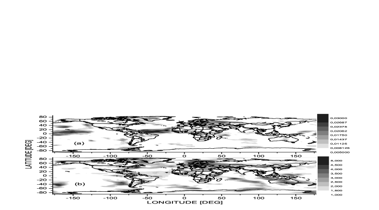
Figure 13: (a) Area weighted connectivity for the scale-specific SATA climate network with the density $\varrho=0.005$ obtained by the uniform thresholding of the MIR (13) estimated using the CCWT within the scales related to the periods 7–8 years. (b) Dependence of the SATA time series on the North Atlantic Oscillation index measured by MIR (13) estimated using the CCWT within the scales related to the periods 7–8 years.

The ENSO is characterized by several indices derived from the sea surface temperature and the Southern Oscillation index (SOI, see http://www.cru.uea.ac.uk/cru/data/soi/ for the data and their description) which is defined as the normalized air pressure difference between Tahiti and Darwin. The MIR quantifying the dependence within the time scales 4–6 years between the SOI and the SATA time series in each grid-point is illustrated in Fig. 12b. The hubs of the SSCN(4–6yr) in the tropical Pacific and Indian Oceans (Fig. 12a) are parts of the areas connected to the ENSO within this time scale (Fig. 12b). However, the areas connected to the ENSO are quite more extended in the Pacific Ocean, tropical Atlantic Ocean and in the Indian and Southern Ocean. Also large continental areas in the Central and Southern America, areas in Africa and some areas in Asia and Northern America have the SATA variability in the time scale 4–6 years connected to the ENSO. This extended ENSO scale-specific connectivity is apparently reflected also in the broad-band connectivity and confirms the role of the hub of the global climate networks for the ENSO tropical Pacific area, as we have observed in the previous Section. The quasi-periodic dynamics plays an important role in the ENSO area temperature variability, e.g. the QQO mode explains almost 40% of the variability of the sea surface temperature anomalies Jiang et al. (1995). This fact explains the low entropy rate of the SATA time series in this area and the dependence between the AWC and the entropy rate in Fig. 11b.

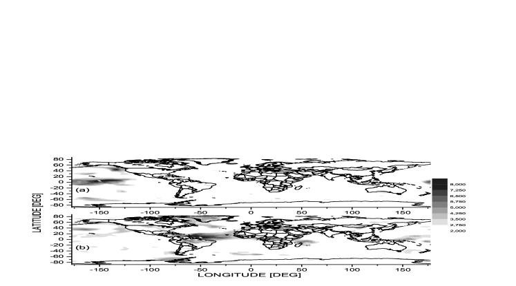
Figure 14: (a) Dependence of the SATA time series from each node with the SATA time series in the node with the longitude 150^∘W and the latitude 5^∘N, measured by MIR (13) estimated using the CCWT within the scales related to periods 7–8 years. (b) The same as in (a), but for the node 50^∘W, 7.5^∘N. The reference node can be seen as a white pixel in the black background.

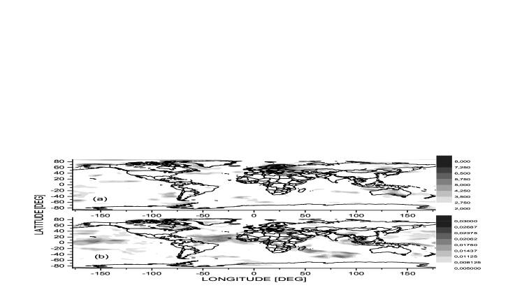
Figure 15: (a) Dependence of the SATA time series from each node with the SATA time series in the node 22.5^∘E, 60^∘N, measured by MIR (13) estimated using the CCWT within the scales related to periods 7–8 years. (b) Area weighted connectivity for the conditional scale-specific SATA climate network with the density $\varrho=0.005$ obtained by the uniform thresholding of the MIR (13) estimated using the CCWT within the scales related to the periods 7–8 years. The MIR between each two nodes is taken conditionally on the NAO index.

Oscillatory phenomena with the period around 7–8 years have been observed in the air temperature and other meteorological data by many authors (see Ref. Paluš and Novotná (2009, 2011) and references therein). Therefore, in the following we will focus on the scale-specific climate network with the connectivity given by the CCWT-based MIR estimate with the wavelet coherence summation restricted to the wavelet scales corresponding to the periods 7–8 years (SSCN(7–8yr) thereafter). Again we consider the binary network with $\varrho=0.005$. The AWC of the SSCN(7–8yr) is mapped in Fig. 13a. Consistently with the observation of the 7–8yr cycle in a number of European locations  Paluš and Novotná (2004, 2007), the SSCN(7–8yr) has a hub in a large area in Europe, but also in Western Asia and Greenland. A strong hub of the SSCN(7–8yr) lies in the tropical Atlantic and also in the Pacific areas different from the ENSO area. The 7–8yr cycle in the European SAT is connected with the North Atlantic Oscillation Paluš and Novotná (2009, 2011).

The North Atlantic Oscillation (NAO) is a dominant pattern of the atmospheric circulation variability in the extratropical Northern Hemisphere. On the global scale, the NAO has a climate significance that rivals the Pacific ENSO Marshall et al. (2001) since it influences the air temperature, precipitation, occurrence of storms, wind strength and direction in the Atlantic sector and surrounding continents. The NAO is characterized by the NAO index (NAOI, see http://www.cru.uea.ac.uk/cru/data/nao/ for the data and their description). While the quasi-periodic dynamics of the ENSO is apparent in the SOI, the NAOI has rather a red-noise-like character Fernandez et al. (2003). However, sensitive detection methods such as the Monte-Carlo singular system analysis Paluš and Novotná (2004) uncovered in the NAO dynamics several oscillatory components from which the cycle with the period around 7–8 years is the most prominent Paluš and Novotná (2007, 2009); Feliks et al. (2010); Paluš and Novotná (2011). The NAO 7–8yr oscillatory mode is phase-synchronized with related modes in the SAT in large areas of Europe Paluš and Novotná (2011) as well as with other weather and climate-related variables in various areas through the Earth Feliks et al. (2010, 2013).

The MIR quantifying the dependence within the time scales 7–8 years between the NAOI and the SATA time series in each grid-point is illustrated in Fig. 13b. We can see that all the hubs in Fig. 13a lie in the areas where the SATA time series are dependent on the NAOI in this scale, with the exception of the Pacific tropical area between 125^∘ – 180^∘W (Fig. 13b). For the better understanding of the topology of the SSCN(7–8yr) we quantify the dependence between the SATA time series in the node 150^∘W, 5^∘N, using the MIR estimated within the wavelet scales related to the periods 7–8 years, see Fig. 14a. Apparently this hub (the Pacific tropical area between 125^∘ – 180^∘W) is connected just with other areas in the Pacific Ocean and disconnected from the rest of the SSCN(7–8yr).

Using the same scale-specific connectivity, we can see that the node at 50^∘W, 7.5^∘N in the tropical Atlantic hub is connected to other hubs of the SSCN(7–8yr), but not to the hub in Europe, see Fig. 14b. (And, of course, the Pacific tropical hub is not connected to any other hub.) The map of the scale-specific connectivity of a node in the European hub (the node 22.5^∘E, 60^∘N lying close to the SW Finland Baltic coast, see Fig. 15a) confirms the disconnection between the tropical Atlantic and the European hubs, however, the latter is connected to many areas all over the world.

The above-mentioned phase synchrony between the 7–8yr oscillatory mode in the NAO and in the European SAT time series evokes the hypothesis that, at least a part of, the connectivity in the SSCN(7–8yr) is induced by the NAO and its world-wide influence. In order to test this hypothesis we construct a version of the scale-specific SSCN(7–8yr) in which, however, the connectivity is given by the scale-specific MIR conditioned on the NAO index. In particular, for each pair of nodes the two SATA time series and the NAOI time series are used to construct the $3\times 3$ wavelet coherence matrix $\Gamma^{W}(f)$ which is then inverted and the MIR conditioned on the NAOI is evaluated according to Eqs. (22) and (23). This measure quantifies the scale-specific dependence between the two SATA series without a possible influence of the NAO 7–8yr oscillatory mode. The AWC map for this conditional SSCN(7–8yr) in Fig. 15b shows that the hub in Europe and W Asia disappears. It means that the scale 7–8yr-specific mutual connectivity of the SATA time series in the areas in Europe and W Asia and their connections to other areas in the world (see Fig. 15a) is induced by the NAO. It is interesting that the hub in the tropical Atlantic survived the conditioning on the NAO, since Feliks et al. Feliks et al. (2010, 2013) track the NAO 7–8yr oscillatory mode to an oscillation of a similar period in the position and strength of the Gulf Stream’s sea surface temperature front in the North Atlantic. The position of the tropical Atlantic hub coincides with the sink region and a warm loop of the Gulf stream. So it seems that the tropical Atlantic area plays a role in the the emergence of the 7–8yr oscillations in nonlinear atmosphere-ocean interactions in the Northern Atlantic, in particular in the dynamics of the NAO. Then the NAO induces this oscillatory mode in temperature variability in large areas in Europe, Asia as well as in other regions in the world (Fig. 13b). These observations concur with some findings of Feliks et al. Feliks et al. (2013) and need further study and understanding. Detailed insight into the related atmospheric circulation phenomena is, however, out of the scope of this paper. Here we wanted to demonstrate the potential of the MIR estimated using the CCWT which gives the possibility to study either the total, or scale-specific or conditional connectivity in networks of interacting dynamical systems or spatio-temporal phenomena in a discrete approximation within the complex networks paradigm.

X Conclusion

Using a simple example of the autoregressive process we have demonstrated how increasing dynamical memory, reflected, e.g., in stronger autocorrelations, leads to increasing bias in estimating dependence measures such as the absolute value of the correlation coefficient. Similar behavior can be observed also in estimates of the mutual information Paluš and Vejmelka (2007), or the mean phase coherence Xu et al. (2006). We have observed how this phenomenon can bias the connectivity in climate networks since the time evolution of the air temperature anomalies, recorded in different geographical areas, have different dynamics. Also in other research fields where interaction/functional networks are inferred from experimental time series this problem can influence the results and skew their interpretation. For instance, many studies of EEG functional networks reported a changed network connectivity in different conscious states, however, changed EEG dynamics had been reported earlier in similar experimental conditions. The mutual information rate can be the dependence measure which can help to distinguish changes in connectivity and long-range synchrony from changes in the dynamics of network nodes. Also other authors Baptista et al. (2012); Blanc et al. (2011) propose the MIR as an association measure suitable for inferring interaction networks from multivariate time series generated by coupled dynamical systems. Blanc et al. Blanc et al. (2011) stress the independence of the MIR of the time lag which can occur between the time evolutions of two interacting systems of processes. This property might be particularly important considering the observation of Martin et al. Martin et al. (2013) regarding the construction of the climate networks from daily air temperature and geopotential height data. Inference of time lags in which the maximum cross-correlation occurs in unreliable and can lead to physically unrealistic large lags and even to the inclusion of non-existing links to the network.

In this paper we have proposed a computationally accessible algorithm based on the MIR of Gaussian processes, adapted by using the wavelet transform. We have demonstrated that this algorithm can be effective for nonlinear, nonstationary and multiscale processes. Using the examples of the climate networks we have presented the ability of the scale-specific and conditional MIR to attribute different hubs of the climate network to different atmospheric circulation phenomena. We believe that the introduced approach can help in further understanding of complex systems and their dynamics which can be observed and recorded in the form of multivariate time series.