Reconnection–Condensation Model for Solar Prominence Formation

Abstract

We propose a reconnection–condensation model in which topological change in a coronal magnetic field via reconnection triggers radiative condensation, thereby resulting in prominence formation. Previous observational studies have suggested that reconnection at a polarity inversion line of a coronal arcade field creates a flux rope that can sustain a prominence; however, they did not explain the origin of cool dense plasmas of prominences. Using three-dimensional magnetohydrodynamic simulations including anisotropic nonlinear thermal conduction and optically thin radiative cooling, we demonstrate that reconnection can lead not only to flux rope formation but also to radiative condensation under a certain condition. In our model, this condition is described by the Field length, which is defined as the scale length for thermal balance between radiative cooling and thermal conduction. This critical condition depends weakly on the artificial background heating. The extreme ultraviolet emissions synthesized with our simulation results have good agreement with observational signatures reported in previous studies.

1 Introduction

Solar prominences, also known as filaments, are cool dense plasma clouds that are typically 100 times cooler and denser than the ambient hot corona. They are one of the basic structures in the corona, and are strongly related to solar eruptions, magnetohydrodynamic (MHD) waves, and coronal heating. Despite the importance of prominences in solar physics, the mechanism of their formation, i.e., the origin of magnetic structures and cool dense plasmas, is not fully understood. Prominences always appear along polarity inversion lines (PILs) across which magnetic polarity at the photosphere is reversed (Martin, 1998; Mackay et al., 2010). Previous observational and theoretical studies proposed that a flux rope sustaining a prominence is formed via magnetic reconnection along a PIL (van Ballegooijen & Martens, 1989; Gaizauskas et al., 1997; Martens & Zwaan, 2001; Yang et al., 2016). However, this reconnection scenario does not explain the origin of cool dense plasmas alone.

Radiative condensation is one mechanism that show promise in explaining how cool dense plasmas are generated in the hot tenuous corona. The observations by the Solar Dynamics Observatory Atmospheric Imaging Assembly (SDO/AIA) revealed a temporal and spatial shift in the peak intensities of multiwavelength extreme ultraviolet (EUV) emissions toward low temperatures during prominence formation events. This could be the evidence for radiative condensation (Berger et al., 2012; Liu et al., 2012).

From a theoretical viewpoint, the corona is thermally unstable even against linear perturbations of sufficiently long wavelength. On the other hand, nonlinear triggers are necessary to grow the thermal instability until the establishment of prominence-corona transition by overcoming the strong stabilizing effect of thermal conduction. Several models involving radiative condensation via nonlinear triggers have been proposed. One such model is the evaporation-condensation model (Mok et al., 1990; Antiochos & Klimchuk, 1991; Antiochos et al., 1999; Karpen et al., 2001, 2003, 2005, 2006; Karpen & Antiochos, 2008; Xia et al., 2011; Luna et al., 2012; Xia et al., 2012; Keppens & Xia, 2014; Xia & Keppens, 2016). In this model, radiative condensation is triggered by an enhancement in the plasma density via an evaporation process driven by strong steady artificial heating at a footpoint of a coronal loop. The crucial factor in this model is steady footpoint heating to drive chromospheric evaporation. An estimation in Aschwanden et al. (2000) using EUV data suggested the presence of nonuniform coronal heating localized at the footpoint of coronal loops. However, hot evaporated flows from the chromosphere have not been detected in prominence formation events.

Other radiative condensation models have adopted reconnection via the footpoint motions of coronal arcade fields as an alternative trigger to evaporation via footpoint heating. A numerical study by Kaneko & Yokoyama (2015) proposed a reconnection–condensation model with in situ radiative condensation triggered by magnetic reconnection. It does not involve any additional artificial footpoint heating or chromospheric evaporation. In this model, a flux rope comprising closed magnetic loops is formed via reconnection. The interior of the closed loops does not gain heat from the exterior via thermal conduction. After suffering a cooling-dominant thermal imbalance, the interior of the closed loops cools continuously until it reaches the temperature of the prominence. This model was demonstrated in Kaneko & Yokoyama (2015) using 2.5-dimensional MHD simulations including optically thin radiative cooling and thermal conduction along magnetic fields. In Linker et al. (2001) and Zhao et al. (2017), prominence formation via direct injection of chromospheric cool plasmas after reconnection was modeled in two-dimensional simulations. These models are not consistent with the in situ condensations observed recently (Berger et al., 2012; Liu et al., 2012). However, it is possible to explain the levitation of chromospheric plasmas with a rising helical flux rope (Okamoto et al., 2008, 2009, 2010).

In this paper, we investigate the reconnection–condensation model using three-dimensional MHD simulations. In the previous simulations performed by Kaneko & Yokoyama (2015), thermal conduction along the axial magnetic fields of a flux rope, which are orthogonal to the simulation domain in their settings, was neglected due to 2.5-dimensional assumption, i.e., temperature gradient perpendicular to the simulation domain was assumed to be zero. In the three-dimensional situation, relaxation via thermal conduction might be more efficient, and there might be a condition whereby radiative condensation is limited by this effect. To check the validity of the reconnection–condensation model and to obtain such a critical condition for prominence formation, we performed three-dimensional MHD simulations including nonlinear anisotropic thermal conduction, optically thin radiative cooling and gravity.

The numerical settings are described in Section 2. In Section 3, the results of the simulations and the images of the EUV emissions synthesized through the filters of SDO/AIA are shown. We discuss the results in Section 4, and a conclusion of the paper is given in Section 5.

2 Numerical Settings

The simulation domain is a rectangular box whose Cartesian coordinates $(x,y,z)$ extend to $-12$ $\mathrm{Mm}<x<12$ $\mathrm{Mm}$, $0<y<40$ $\mathrm{Mm}$, and $0<z<65$ $\mathrm{Mm}$, where the $y$-direction corresponds to the height and the $xz$-plane is parallel to the horizontal plane.

The initial corona is under hydrostatic stratification with a uniform temperature ($T_{\mathrm{cor}}=1~{}\mathrm{MK}$) and a uniform gravity ($g_{\mathrm{cor}}=270~{}\mathrm{m/s^{2}}$). The initial density profile is given as

$$n=n_{\mathrm{cor}}\exp\left[-\frac{y}{L_{s}}\right],$$ (1)

where $n$ is number density, $n_{\mathrm{cor}}=10^{9}~{}\mathrm{cm^{-3}}$ is the number density at $y=0$ and $L_{s}=k_{B}T_{\mathrm{cor}}/(mg_{\mathrm{cor}})=30~{}\mathrm{Mm}$ is the coronal scale height. The initial magnetic field is a linear force-free arcade and is given as

$$B_{x} = -\left(\frac{2L_{a}}{\pi a}\right)B_{a}\cos\left(\frac{\pi x}{2L_{a}}\right)\exp\left[-\frac{y}{a}\right],$$ (2)

$$B_{y} = B_{a}\sin\left(\frac{\pi x}{2L_{a}}\right)\exp\left[-\frac{y}{a}\right],$$ (3)

$$B_{z} = -\sqrt{1-\left(\frac{2L_{a}}{\pi a}\right)^{2}}B_{a}\cos\left(\frac{\pi x}{2L_{a}}\right)\exp\left[-\frac{y}{a}\right],$$ (4)

where $B_{a}=6~{}\mathrm{G}$, $L_{a}=12~{}\mathrm{Mm}$, and $a=30~{}\mathrm{Mm}$ (see Fig. 1 (a)). The PIL is located at $x=0$. The three-dimensional MHD equations including nonlinear anisotropic thermal conduction and optically thin radiative cooling are solved numerically as follows:

$$\frac{\partial\rho}{\partial t}+\nabla\cdot\left(\rho\mbox{\boldmath$v$}\right)=0,$$ (5)

$$\frac{\partial\left(\rho\mbox{\boldmath$v$}\right)}{\partial t}+\nabla\cdot\left(\rho\mbox{\boldmath$v$}\mbox{\boldmath$v$}+p\mbox{\boldmath$I$}-\frac{\mbox{\boldmath$B$}\mbox{\boldmath$B$}}{4\pi}+\frac{B^{2}}{8\pi}\mbox{\boldmath$I$}\right)-\rho\mbox{\boldmath$g$}=0,$$ (6)

$$\frac{\partial}{\partial t}\left(e_{\mathrm{th}}+\frac{1}{2}\rho\mbox{\boldmath$v$}^{2}+\frac{B^{2}}{8\pi}\right)+\nabla\cdot\left[\left(e_{\mathrm{th}}+p+\frac{1}{2}\rho\mbox{\boldmath$v$}^{2}\right)\mbox{\boldmath$v$}+\frac{c}{4\pi}\mbox{\boldmath$E$}\times\mbox{\boldmath$B$}\right]$$

$$=\rho\mbox{\boldmath$g$}\cdot\mbox{\boldmath$v$}+\nabla\cdot\left(\kappa T^{5/2}\mbox{\boldmath$b$}\mbox{\boldmath$b$}\cdot\nabla T\right)-n^{2}\Lambda(T)+H,$$ (7)

$$e_{\mathrm{th}}=\frac{p}{\gamma-1},$$ (8)

$$T=\frac{m}{k_{B}}\frac{p}{\rho},$$ (9)

$$\frac{\partial\mbox{\boldmath$B$}}{\partial t}=-c\nabla\times\mbox{\boldmath$E$},$$ (10)

$$\mbox{\boldmath$E$}=-\frac{1}{c}\mbox{\boldmath$v$}\times\mbox{\boldmath$B$}+\frac{4\pi\eta}{c^{2}}\mbox{\boldmath$J$},$$ (11)

$$\mbox{\boldmath$J$}=\frac{c}{4\pi}\nabla\times\mbox{\boldmath$B$},$$ (12)

where $\mathrm{\kappa=2\times 10^{-6}~{}erg~{}cm^{-1}~{}s^{-1}~{}K^{-7/2}}$ is the coefficient of thermal conduction, $b$ is a unit vector along the magnetic field, $\Lambda(T)$ is the radiative loss function of optically thin plasma, $H$ is the background heating rate, and $\eta$ is the magnetic diffusion rate. We use the same radiative loss function as that used in Kaneko & Yokoyama (2015). However, there is no temperature cutoff, rather, we assume a dependence of $T^{3}$ below $10^{4}~{}\mathrm{K}$. To achieve the initial thermal equilibrium, the background coronal heating proportional to the magnetic energy density is set to $H=\alpha_{A}B^{2}$, where $B$ is the magnetic field strength and $\alpha_{A}=1.5\times 10^{-6}~{}\mathrm{s^{-1}}$ is a constant coefficient. Note that $\alpha_{A}$ can be a constant because the coronal scale height $L_{s}$ is the same as the magnetic decay length $a$ such that

$$n^{2}\Lambda(T_{\mathrm{cor}})=H$$ (13)

$$\Leftrightarrow n_{\mathrm{cor}}^{2}\Lambda(T_{\mathrm{cor}})\exp\left[\frac{2y}{L_{s}}\right]=\alpha_{A}B_{a}^{2}\exp\left[\frac{2y}{a}\right]$$ (14)

$$\Leftrightarrow \alpha_{A}=\frac{n_{\mathrm{cor}}^{2}\Lambda(T_{\mathrm{cor}})}{B_{a}^{2}}.$$ (15)

For fast magnetic reconnection, we adopt the following form of the anomalous resistivity (e.g. Yokoyama & Shibata, 1994):

$$\eta = 0,~{}~{}~{}\left(J<J_{c}\right)$$ (16)

$$\eta = \eta_{0}\left(J/J_{c}-1\right)^{2},~{}~{}~{}\left(J\geq J_{c}\right)$$ (17)

where $\eta_{0}=\mathrm{3.6\times 10^{13}~{}cm^{2}~{}s^{-1}}$ and $J_{c}=\mathrm{25~{}erg^{1/2}~{}cm^{-3/2}~{}s^{-1}}$. We restrict $\eta$ to $\eta_{\mathrm{max}}=\mathrm{1.8\times 10^{14}~{}cm^{2}~{}s^{-1}}$. To drive reconnection at the PIL of the arcade field, footpoint velocities perpendicular and parallel to the PIL are given as

$$v_{x} = -v_{0}(t)\sin\left(\frac{\pi x}{2L_{a}}\right)\exp\left[-\left(\frac{z}{L_{a}}\right)^{2}\right],$$ (18)

$$v_{y} = 0,$$ (19)

$$v_{z} = v_{x},$$ (20)

where $t$ represents time, and $v_{0}(t)$, the speed dependent on time, is set in the region below $y=0$. The speed $v_{0}(t)$ is given as

$$v_{0}(t) = v_{00},~{}~{}(0<t<t_{1})$$ (21)

$$v_{0}(t) = v_{00}\frac{t_{2}-t}{t_{2}-t_{1}},~{}~{}(t_{1}\leq t<t_{2})$$ (22)

$$v_{0}(t) = 0,~{}~{}(t\geq t_{2})$$ (23)

where $v_{00}=6~{}\mathrm{km/s}$, $t_{1}=4320~{}\mathrm{s}$, and $t_{2}=4560~{}\mathrm{s}$. In the numerical study by Kaneko & Yokoyama (2015), a parameter survey on the direction of parallel motion was performed using 2.5-dimensional simulations. They concluded that radiative condensation is more likely to occur in the case of anti-shearing motion (in which the direction of parallel motion is opposite to that of the magnetic shear) rather than in the case of shearing motion (in which the direction of parallel motion is the same as that of the magnetic shear). In the present study, we investigate the cases of anti-shearing motion using three-dimensional simulations. The magnetic fields below $y=0$ are computed by the induction equation with the footpoint velocities given as Eqs. (18) - (23). The free boundary condition is applied to the magnetic fields at the lower boundary. The gas pressure and density below $y=0$ are assumed to be unchanged in hydrostatic equilibrium at a uniform temperature of $1~{}\mathrm{MK}$. The free boundary condition is applied to all the variables at the upper boundary. The anti-symmetric boundary condition is applied to $v_{x},v_{z},B_{x},$ and $B_{z}$, and the symmetric boundary condition is applied to the other variables at the boundaries in the $x$-direction. Because the system evolves in two-fold rotational symmetry around the $y$-axis at $(x,z)=0$, we set symmetry boundary condition for a rotation of 180 degrees in the $xy$-plain at $z=0$ to reduce numerical amount. We also assume the same rotational symmetry at $(x,z)=(0,65~{}\mathrm{Mm})$. In the following figures, plots in the range of $-65~{}\mathrm{Mm}<z<65~{}\mathrm{Mm}$ are shown.

The numerical scheme is a four-stage Runge–Kutta method (Vögler et al., 2005) and a fourth-order central finite difference method with artificial viscosity (Rempel, 2014). Thermal conduction is explicitly solved using a super-time-stepping method with second-order temporal and spatial accuracy (Meyer et al., 2012, 2014). The grid spacing size is $120$ $\mathrm{km}$ everywhere.

3 Results

Figures 1 and 2 are snapshots of our simulation result. The initial arcade field (Fig. 1 (a)) evolves into a flux rope structure owing to reconnection via the footpoint motion (Fig. 1 (b)). The flux rope traps dense plasmas at the lower corona, and the radiative cooling inside the flux rope overwhelms the background heating. Owing to reconnection, the length of the magnetic loops becomes longer, and the relaxation effect of thermal conduction along the long magnetic loops becomes weaker. The enhanced radiative loss is not fully compensated for by the thermal conduction along the long reconnected magnetic loops, leading to radiative condensation (Fig. 2 (a)). The condensed plasmas are accumulated into the magnetic dips of the flux rope because of gravity. Owing to the location of the dips, the dense plasmas concentrate above the PIL to form a filament structure as shown in the top view of Fig. 2 (b).

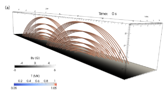
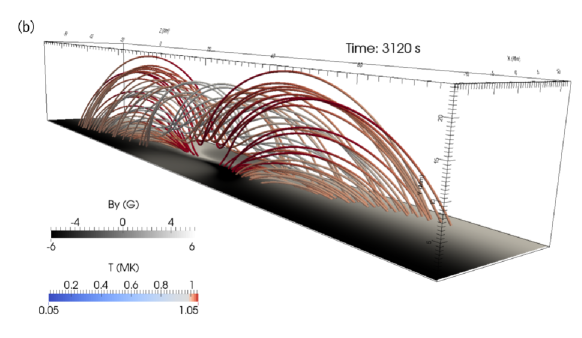
Figure 1: Simulation results. Panel (a) shows the initial condition. Panel (b) shows the snapshot after the formation of a flux rope. The lines indicate the magnetic field and their color represents the temperature. The grayscale at the bottom boundary represents the signed strength of the magnetic field perpendicular to the surface.

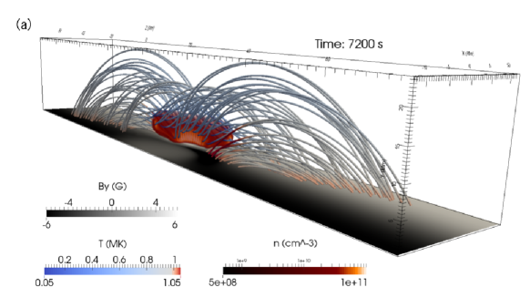
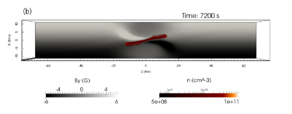
Figure 2: Simulation results after radiative condensation. Panel (a) shows a side view with the magnetic field lines, and Panel (b) shows the top view without magnetic field lines. The area with a high density ($n>4.0\times 10^{9}~{}\mathrm{cm^{-3}}$) is shown in red volume rendering. The lines, colors, and grayscale represent the same as those shown in Fig. 1.

Figure 3 shows the density distribution at $t=3120~{}\mathrm{s}$ in the $xy$-plain at $z=0$ with magnetic field lines of the flux rope. The dense plasmas initially at the lower altitude are trapped: they are subsequently lifted up by the ascending flux rope. Figure 4 shows the profiles of cooling rate, heating rate, and density along $y$-axis in the $xy$-plane. The cooling rate is enhanced by the dense plasmas trapped inside the flux rope ($y=3-13~{}\mathrm{Mm}$), and it overwhelms the background heating rate. The enhanced radiative loss inside the flux rope is the source of radiative condensation.

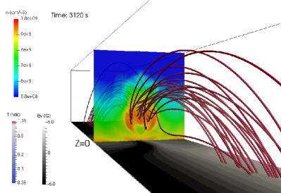
Figure 3: Density distribution inside the flux rope at $t=3120~{}\mathrm{s}$. Colors on the $xy$-plane at $z=0$ represent density. The lines and grayscale at the bottom boundary represent the same as those in Fig. 1.

Figure 4: Cooling and heating rate along the $y$-axis in the $xy$-plane at $z=0$ and $t=3120~{}\mathrm{s}$. Solid and dashed lines represent the cooling and heating rates, respectively. The dash-dotted line represents the density profile.

The relationship between the length and the minimum temperature is shown in Fig. 5 for each individual magnetic field line. At the initial state, the temperature is uniform at $10^{6}~{}\mathrm{MK}$ (black crosses in Fig. 5). The loop length becomes roughly double after reconnection ($t=3120$ s, red triangles), and the longer loops suffer from radiative condensation ($t=7200$ s, blue squares). The critical length for radiative condensation can be explained by the Field length (Field, 1965), which given as

$$\lambda_{F}(T,n)\approx\sqrt{\frac{\kappa T^{7/2}}{n^{2}\Lambda(T)}},$$ (24)

and the critical condition is

$$L>\lambda_{F},$$ (25)

where $L$ is the length of the magnetic loops. The solid and dashed lines in Fig. 5 represent the Field lengths $\lambda_{F}(T,n_{t})$ and $\lambda_{F}(T,n_{b})$, where $n_{t}=5.0\times 10^{8}~{}\mathrm{cm^{-3}}$ and $n_{b}=1.0\times 10^{9}~{}\mathrm{cm^{-3}}$ are the densities around the top of the tallest arcades subject to reconnection, and at the bottom boundary, respectively. The possible criteria in Fig. 5 are estimated based on maximum thermal conduction effect (of $1~{}\mathrm{MK}$) versus possible variation of radiative cooling associated with the density profile along the field lines. Our simulation results show that the Field length can approximately explain the condition of radiative condensation.

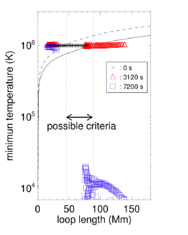
Figure 5: Relationship between the loop length and the minimum temperature of individual magnetic loops at different times. Solid and dashed lines represent $\lambda_{F}(T,n_{t})$ and $\lambda_{F}(T,n_{b})$ respectively. Black crosses, red triangles and blue squares represent the state at the different times, as shown in the inset.

Figure 6 shows the EUV emissions synthesized through the filters of SDO/AIA. A dark cavity surrounding the prominence is formed in the emissions of the coronal temperatures at 193 and 171 $\mathrm{\AA}$. A low density cavity is formed as a natural consequence of mass conservation because all the prominence mass in our model comes from the surrounding corona. In Fig. 7 (a), the regions surrounded by blue surfaces represent the three-dimensional morphology of the cavity in our simulation. We find that the shape of the cavity resembles the wing of a seagull: this is because the cavity is formed along the sheared coronal magnetic field lines. As shown in Fig. 7 (b), temperature inside the cavity ranges from $0.6$ to $1.0~{}\mathrm{MK}$. The variation of temperature has little influence on the shape of the cavity in 193 $\mathrm{\AA}$, because the temperature response function is almost constant in this range of temperature. The variation of temperature can affect the shape of the cavity in 171 $\mathrm{\AA}$ where the response function has a peak around $0.8~{}\mathrm{MK}$ and is not constant. However, the shape of cavity in $171~{}\mathrm{\AA}$ is quite similar to that in $193~{}\mathrm{\AA}$ (see Fig. 6 (b) and (c)). It is concluded that the depletion of mass mostly contributes to the formation of the cavity. The maximum density and the minimum temperature of our simulated prominence are $10^{11}~{}\mathrm{cm^{-3}}$ and $0.06~{}\mathrm{MK}$, which are $100$ times higher and lower than those in the initial corona, respectively. The averaged density and the volume in the region where temperature is lower than $0.1~{}\mathrm{MK}$ are $2\times 10^{10}~{}\mathrm{cm^{-3}}$ and $8\times 10^{26}~{}\mathrm{cm^{3}}$, respectively. Although our model does not include the chromosphere, the resultant mass reaches the observed lower limit of typical prominence densities and volumes (Labrosse et al., 2010). This is because the volume of the cavity is much larger than that of the prominence, as shown in Fig. 7. Figure 8 shows the time evolution of the EUV emissions. During radiative condensation, the intensity peak shows a temporal shift from 171 $\mathrm{\AA}$ (coronal temperature) to 304 $\mathrm{\AA}$ (prominence temperature), which is qualitatively consistent with the observations made by Berger et al. (2012). The time scale until condensation starts in our simulation is rather closer to that in active regions (several tens of minutes, Yang et al., 2016) than that in quiet regions (several hours, Berger et al., 2012; Liu et al., 2012). This is because the initial density in our simulations ($5-10\times 10^{8}~{}\mathrm{cm^{-3}}$) is higher than the typical coronal density in quiet regions ($10^{8}~{}\mathrm{cm^{-3}}$). Note that the 211 $\mathrm{\AA}$ filter image is not synthesized here because the initial coronal temperature is $1~{}\mathrm{MK}$ in our simulation. A 131 $\mathrm{\AA}$ filtergram is used as the signature of the transition temperature between the corona and the prominence. The 193 $\mathrm{\AA}$ emission is bright during the reconnection phase ($t=10$ - $20~{}\mathrm{min}$), which reflects the temperature increase from $1~{}\mathrm{MK}$ to $1.2~{}\mathrm{MK}$ inside the flux rope via reconnection heating and the density increase via the levitation of the lower coronal plasma.

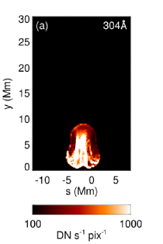
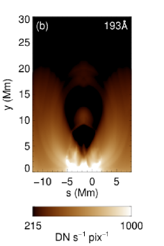
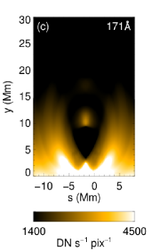
Figure 6: EUV emission synthesized through the SDO/AIA filters at $t=7200~{}\mathrm{s}$. Panels (a), (b) and (c) represent the images obtained at $304\mathrm{\AA}$, $193\mathrm{\AA}$, and $131\mathrm{\AA}$, respectively. The angle between the line of sight and the $z$-axis is chosen to be $5^{\circ}$ for the synthesis. The coordinate $s$ is inclined at $5^{\circ}$ to the $x$-axis.

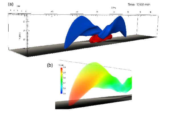
Figure 7: Panel (a) : three-dimensional morphology of the cavity and prominence. Blue and red contours represent density surface of $n=3.5\times 10^{8}~{}\mathrm{cm^{-3}}$ and $n=1.0\times 10^{10}~{}\mathrm{cm^{-3}}$, respectively. Panel (b) : distribution of temperature inside the cavity shown by volume rendering.

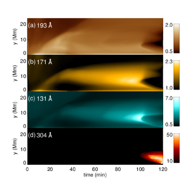
Figure 8: Time–height plot of the synthesized EUV emission ratios through SDO/AIA filters. The emission in the region from $s=-5~{}\mathrm{Mm}$ to $2~{}\mathrm{Mm}$ in Fig. 6 is averaged. The emission at time = 0 s is the reference of the ratio for each filter. Panels (a), (b), (c), and (d) represent the images of $193~{}\mathrm{\AA}$, $171~{}\mathrm{\AA}$, $131~{}\mathrm{\AA}$, and $304~{}\mathrm{\AA}$, respectively.

4 Discussion

Our study propose a new possible process to meet the condition for thermal instability in the magnetized plasma compared to the previous models, e.g., evaporation–condensation model. In our reconnection–condensation model, the length of the magnetic loops exceeds the Field length as a result of magnetic reconnection. The Field length in our model depends on the density and temperature, which are nearly unchanged from those in the initial coronal state. On the other hand, in the evaporation–condensation model, the loop length does not change and the Field length becomes shorter owing to mass supply from the evaporated flows (Xia et al., 2011). These two different routes to condensation can both occur in actual solar atmospheres. We speculate that our reconnection–condensation model is more appropriate to explain prominence formation in quiet regions where the strong evaporation can not be expected.

Future observational studies should investigate the length of reconnected loops in terms of their extension beyond the Field length. The Field length is longer in quiet regions and shorter in active regions owing to differences in the typical densities. This may explain the difference between typical length of quiescent prominences ($\sim 100~{}\mathrm{Mm}$) and active region prominences ($\sim 10~{}\mathrm{Mm}$).

A possible origin of the converging and anti-shearing motions is the interaction of diverging flows of supergranules crossing a PIL (Rondi et al., 2007; Schmieder et al., 2014), which have a mean speed of $0.3~{}\mathrm{km/s}$. Because the typical lifetime of supergranules is one day, the migration distance of a magnetic element is approximately $20~{}\mathrm{Mm}$. In this study, we use a footpoint motion with a speed of $6~{}\mathrm{km/s}$ for $4000~{}\mathrm{s}$. Because the migration distance is consistent with the observational values, the amount of reconnected fluxes in our simulations is reasonable. We speculate that both anti-shearing and shearing motions are created depending on the relative position of supergranules against the direction of the magnetic shear of the filament channel, as shown in Fig. 9. The results of a parameter survey conducted in Kaneko & Yokoyama (2015) show that anti-shearing results in radiative condensation, whereas shearing causes eruptions. Future observational studies on filament formation should investigate the distribution of supergranules around filament channels.

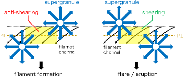
Figure 9: Possible relationship between the relative position of supergranules and the direction of footpoint motion. The top view of filament channels is shown, and black curved arrows represent magnetic fields. Blue arrows represent diverging flows of the supergranules. Yellow regions suffer from converging motion and anti-shearing or shearing motion depending on relative position of the supergranules.

To check the dependence on the artificial background heating, we performed an additional simulation using a different type of background heating, $H=\alpha_{B}nB$, where $\alpha_{B}=9.2\times 10^{-15}~{}\mathrm{erg^{-1/2}~{}cm^{-3/2}~{}s^{-1}}$ is set for the initial thermal balance. Figure 10 shows relationship between the loop length and the minimum temperature of magnetic loops. The critical condition of the Field length is valid even in this heating model. By comparing the results of two different heating models, we find a common tendency that the longer loops reach the lower temperatures (see blue squares in Figs. 5 and 10). This is because the stabilizing effect of thermal conduction is weaker in the longer loops. The deviation from this tendency in the shorter loops can be a multi-dimensional effect, where, as the prominence descends by gravity, the shorter loops below the prominence start to condense due to compression. A difference between the results of two heating models is the temperature of prominences. The prominence temperature in the heating model of $H=\alpha_{B}nB$ is higher because the heating rate inside the prominence increases as the density increases. In this study, we examined only two heating models. In future, other types of heating models proposed by previous studies (Mandrini et al., 2000) need to be investigated. Simulation of condensation using a self-consistent coronal heating model is also a candidate for future studies.

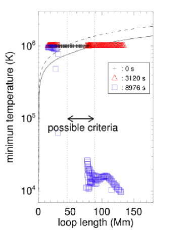
Figure 10: Relationship between the loop length and the minimum temperature of individual magnetic loops in the case of heating model $H=\alpha_{B}nB$. Black crosses, red triangles and blue squares represent the state at the different times, as shown in the inset. Solid and dashed lines represent the same as those shown in Fig. 5.

As mentioned in Section 3, the mass of our simulated prominence satisfies only the lower limit of the typical prominence mass. To obtain more mass, one possible approach is to construct a longer flux rope using multiple reconnections. Because several converging points are observed around PILs owing to the interactions between supergranules (Schmieder et al., 2014), multiple reconnection events are plausible. Another possibility is an additional mass supply from chromospheric jets (Chae, 2003) or a siphon-like mechanism driven by a strong pressure gradient during condensation (Poland & Mariska, 1986; Choe & Lee, 1992; Karpen et al., 2001; Xia et al., 2011).

Understanding the mechanism of mass circulation between the corona, prominences and the chromosphere is an important issue when discussing the mass budget of prominences and coronal mass ejections (CMEs). This issue may also be related to the mechanisms of recurrent prominence formation and homologous CMEs. A numerical simulation by Xia & Keppens (2016) reproduced a prominence with fragmented interior structures and indicated that a continuous mass supply via evaporation can sustain the mass cycle between the chromosphere and the corona via prominences, however, such a steady strong evaporation has not yet been observed. In our study, the simulated prominence did not show interior fine structures reported in the previous studies (Berger et al., 2008; Hillier et al., 2012; Keppens et al., 2015). Perturbations to trigger the Rayleigh-Taylor instability might be necessary. In addition, our model excludes the chromosphere, and the transfer of mass occurs only from the corona to the prominence. To discuss the mass transport system, our model must include the chromosphere in the future.

The reconnection model can affect the initiation of prominence eruption. In our simulations, the flux rope was elevated by the Petschek type fast reconnection after anomalous resistivity was swiched on; however, it did not erupt. Figure 11 shows snapshots of current density in the $xy$-plane at $z=0$ at different times. After the onset of reconnection via converging motion, a localized current sheet typical for the Petschek type reconnection was created (Fig. 11 (a)). The strong current gradually faded away as magnetic flux inside the converging area was depleted (Fig. 11 (b)). The anti-shearing motion also reduced current density. Eventually, the anomalous resistivity was switched off, and the elevation of the flux rope was stopped. 2.5-dimensional MHD simulation using uniform resistivity in Zhao et al. (2017) succeeded in reproducing prominence eruption by reconnection via converging motion. In their study, reconnection burst by plasmoid instability in a long current sheet accelerated the flux rope, leading to eruptions. Thus the detail of reconnection (or resistivity) model is one important factor to understand the eruptive mechanism of prominences.

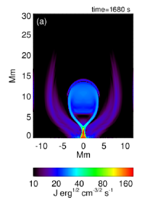
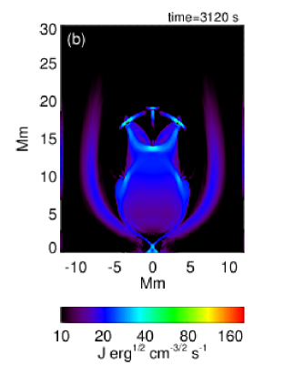
Figure 11: Current density in $xy$-plane at $z=0$.

5 Conclusion

We demonstrated a reconnection–condensation model for solar prominence formation using three-dimensional MHD simulations including nonlinear anisotropic thermal conduction and optically thin radiative cooling. In this model, reconnection and the subsequent topological change in the magnetic field cause radiative condensation. When the length of the reconnected loops exceeds the Field length, radiative condensation is triggered. The synthesized images of EUV emissions are consistent with the observational findings, i.e., in terms of the temporal and spatial shift in the peak intensities of multiwavelength EUV emissions from coronal temperatures to prominence temperatures and the formation of a dark cavity. Previous studies have proposed a reconnection scenario for the formation of a flux rope sustaining a prominence (van Ballegooijen & Martens, 1989; Martens & Zwaan, 2001; Welsch et al., 2005); however, these studies have not been able to explain the origin of cool dense plasmas in this reconnection scenario alone. Our study provides a clear link between reconnection and radiative condensation and verifies that reconnection leads not only to the flux rope formation but also to the generation of cool dense plasmas of prominences under the condition associated with the Field length.

References

- Antiochos & Klimchuk (1991) Antiochos, S. K., & Klimchuk, J. A. 1991, ApJ, 378, 372
- Antiochos et al. (1999) Antiochos, S. K., MacNeice, P. J., Spicer, D. S., & Klimchuk, J. A. 1999, ApJ, 512, 985
- Aschwanden et al. (2000) Aschwanden, M. J., Nightingale, R. W., & Alexander, D. 2000, ApJ, 541, 1059
- Berger et al. (2012) Berger, T. E., Liu, W., & Low, B. C. 2012, ApJ, 758, L37
- Berger et al. (2008) Berger, T. E., Shine, R. A., Slater, G. L., et al. 2008, ApJ, 676, L89
- Chae (2003) Chae, J. 2003, ApJ, 584, 1084
- Choe & Lee (1992) Choe, G. S., & Lee, L. C. 1992, Sol. Phys., 138, 291
- Field (1965) Field, G. B. 1965, ApJ, 142, 531
- Gaizauskas et al. (1997) Gaizauskas, V., Zirker, J. B., Sweetland, C., & Kovacs, A. 1997, ApJ, 479, 448
- Hillier et al. (2012) Hillier, A., Berger, T., Isobe, H., & Shibata, K. 2012, ApJ, 746, 120
- Kaneko & Yokoyama (2015) Kaneko, T., & Yokoyama, T. 2015, ApJ, 806, 115
- Karpen & Antiochos (2008) Karpen, J. T., & Antiochos, S. K. 2008, ApJ, 676, 658
- Karpen et al. (2001) Karpen, J. T., Antiochos, S. K., Hohensee, M., Klimchuk, J. A., & MacNeice, P. J. 2001, ApJ, 553, L85
- Karpen et al. (2006) Karpen, J. T., Antiochos, S. K., & Klimchuk, J. A. 2006, ApJ, 637, 531
- Karpen et al. (2003) Karpen, J. T., Antiochos, S. K., Klimchuk, J. A., & MacNeice, P. J. 2003, ApJ, 593, 1187
- Karpen et al. (2005) Karpen, J. T., Tanner, S. E. M., Antiochos, S. K., & DeVore, C. R. 2005, ApJ, 635, 1319
- Keppens & Xia (2014) Keppens, R., & Xia, C. 2014, ApJ, 789, 22
- Keppens et al. (2015) Keppens, R., Xia, C., & Porth, O. 2015, ApJ, 806, L13
- Labrosse et al. (2010) Labrosse, N., Heinzel, P., Vial, J.-C., et al. 2010, Space Sci. Rev., 151, 243
- Linker et al. (2001) Linker, J. A., Lionello, R., Mikić, Z., & Amari, T. 2001, J. Geophys. Res., 106, 25165
- Liu et al. (2012) Liu, W., Berger, T. E., & Low, B. C. 2012, ApJ, 745, L21
- Luna et al. (2012) Luna, M., Karpen, J. T., & DeVore, C. R. 2012, ApJ, 746, 30
- Mackay et al. (2010) Mackay, D. H., Karpen, J. T., Ballester, J. L., Schmieder, B., & Aulanier, G. 2010, Space Sci. Rev., 151, 333
- Mandrini et al. (2000) Mandrini, C. H., Démoulin, P., & Klimchuk, J. A. 2000, ApJ, 530, 999
- Martens & Zwaan (2001) Martens, P. C., & Zwaan, C. 2001, ApJ, 558, 872
- Martin (1998) Martin, S. F. 1998, Sol. Phys., 182, 107
- Meyer et al. (2012) Meyer, C. D., Balsara, D. S., & Aslam, T. D. 2012, MNRAS, 422, 2102
- Meyer et al. (2014) Meyer, C. D., Balsara, D. S., & Aslam, T. D. 2014, Journal of Computational Physics, 257, 594
- Mok et al. (1990) Mok, Y., Drake, J. F., Schnack, D. D., & van Hoven, G. 1990, ApJ, 359, 228
- Okamoto et al. (2010) Okamoto, T. J., Tsuneta, S., & Berger, T. E. 2010, ApJ, 719, 583
- Okamoto et al. (2008) Okamoto, T. J., Tsuneta, S., Lites, B. W., et al. 2008, ApJ, 673, L215
- Okamoto et al. (2009) —. 2009, ApJ, 697, 913
- Poland & Mariska (1986) Poland, A. I., & Mariska, J. T. 1986, Sol. Phys., 104, 303
- Rempel (2014) Rempel, M. 2014, ApJ, 789, 132
- Rondi et al. (2007) Rondi, S., Roudier, T., Molodij, G., et al. 2007, A&A, 467, 1289
- Schmieder et al. (2014) Schmieder, B., Roudier, T., Mein, N., et al. 2014, A&A, 564, A104
- van Ballegooijen & Martens (1989) van Ballegooijen, A. A., & Martens, P. C. H. 1989, ApJ, 343, 971
- Vögler et al. (2005) Vögler, A., Shelyag, S., Schüssler, M., et al. 2005, A&A, 429, 335
- Welsch et al. (2005) Welsch, B. T., DeVore, C. R., & Antiochos, S. K. 2005, ApJ, 634, 1395
- Xia et al. (2012) Xia, C., Chen, P. F., & Keppens, R. 2012, ApJ, 748, L26
- Xia et al. (2011) Xia, C., Chen, P. F., Keppens, R., & van Marle, A. J. 2011, ApJ, 737, 27
- Xia & Keppens (2016) Xia, C., & Keppens, R. 2016, ApJ, 823, 22
- Yang et al. (2016) Yang, B., Jiang, Y., Yang, J., Yu, S., & Xu, Z. 2016, ApJ, 816, 41
- Yokoyama & Shibata (1994) Yokoyama, T., & Shibata, K. 1994, ApJ, 436, L197
- Zhao et al. (2017) Zhao, X., Xia, C., Keppens, R., & Gan, W. 2017, ApJ, 841, 106