Towards Bursting Filter Bubble
via Contextual Risks and Uncertainties
Abstract
A rising topic in computational journalism is how to enhance the diversity in news served to subscribers to foster exploration behavior in news reading. Despite the success of preference learning in personalized news recommendation, their over-exploitation causes filter bubble that isolates readers from opposing viewpoints and hurts long-term user experiences with lack of serendipity. Since news providers can recommend neither opposite nor diversified opinions if unpopularity of these articles is surely predicted, they can only bet on the articles whose forecasts of click-through rate involve high variability (risks) or high estimation errors (uncertainties). We propose a novel Bayesian model of uncertainty-aware scoring and ranking for news articles. The Bayesian binary classifier models probability of success (defined as a news click) as a Beta-distributed random variable conditional on a vector of the context (user features, article features, and other contextual features). The posterior of the contextual coefficients can be computed efficiently using a low-rank version of Laplace’s method via thin Singular Value Decomposition. Efficiencies in personalized targeting of exceptional articles, which are chosen by each subscriber in test period, are evaluated on real-world news datasets. The proposed estimator slightly outperformed existing training and scoring algorithms, in terms of efficiency in identifying successful outliers.
1 Introduction
Personalized news recommendation has been a successful application of machine learning although it would also endanger people’s open-mindedness towards opposing viewpoints. Targeted news delivery has been reinforced by collections of click response logs, with preference learning algorithms such as bilinear models [1, 2], topic models [3], matrix factorization [4, 5, 6], learning to rank [7], or their hybrid [8, 9]. In terms of exploration-exploitation trade-off, however, the exploitative nature of data-oriented personalization has been criticized as a cause of the filter bubble [10], which is a compound problem fueled both by narrow-minded human’s willing choice [11] and by machines over-confident about their scoring. In this paper, we address the problem of over-confident machines while psychologically opening people’s mind is out of the current scope.
Even by diversifying recommendations or by exploring around uncertain preferences, online news providers cannot deliver articles whose unpopularity is surely predicted. Submodular maximization algorithms [12] or Determinantal Point Processes (DPPs [13, 14, 15]; see [16] for good summary) generate a subset of input items associated with univariate scores (e.g., estimated click-through rates). The output subset consists of some high-score items that are well diversified. Unfortunately, due to the exclusion of low-score items, diversification algorithms never select items whose unpopularity is statistically significant. Another direction towards serendipity is to use not unbiased but optimistically-biased estimates as in contextual multi-armed bandit algorithms [17, 18, 12, 19, 20]. Bandit algorithms, however, also fail to select surely unpopular items, because expected cumulative reward is their main objective in repeated trials. As a consequence, as long as a large number of total clicks must be retained, news providers cannot bet against readers’ preference evidenced by large samples.
We instead recommend articles whose popularity involves high variabilities (risks) and/or high estimation errors (uncertainties), by introducing a new Bayesian classifier that explicitly formalizes the dependence of variabilities on recommendation contexts. It is worth observing that Maximum A Posteriori (MAP) point estimation and logistic-loss models (e.g., factorization machines [21, 22] and deep neural networks [23]) are broadly used in real-world systems. We hypothesize that content providers too much rely on the logistic-loss MAP estimates because of their successes in retrieving popular items, and they often forget the fact that substance of their model is an erroneous estimate deviated from the true preference. Furthermore, we gaze at a statistical insight that estimation error of variability statistic is particularly high when the true variability is high. By performing Bayesian interval estimation and assuming the true variability to be a function of context, we robustly quantify the total stochasticity with clear separation between the essential variability and estimation error. These deliberated philosophies behind our model are expected to increase the chance of discovering exceptional items, whose preference uncertainty has been underestimated by the existing models.
Our key ideas to accurately quantify the context-dependent risks and uncertainties are conditional Beta distribution and low-rank Laplace approximation with affordable computational costs. We model the probability of success as a random variable to obey a Beta distribution, whose two parameters are both functions of input vector. In training, we approximate the posterior by a low-rank Gaussian distribution whose estimates of the variance-covariance matrices are given by thin Singular Value Decomposition (SVD). Thanks to this thin SVD, we can perform both training and recommendation efficiently by sparse high-dimensional matrix libraries. We also derive a variety of uncertainty-aware scoring measures over the closed forms of the approximate posterior, and evaluate the performance of every measure by using real-world news-reading datasets. While we compare linear models in the experiments, since our model is a robust extension of logistic regression with additional dispersion parameters, the principle of combining conditional Beta distribution with low-rank Laplace’s method is broadly pluggable into many logistic-loss non-linear models.
The remainder of this paper is organized as follows. Our Bayesian binary classifier and its approximate posterior inference are introduced in Section 2. We then derive several types of posterior-based scoring methods in Section 3. Section 4 discusses the related work on robust classification and human’s exploration behavior though the latter theme is out of our scope. In Section 5, we numerically evaluate the proposed algorithm and scoring measures for the news datasets, with introducing a novel performance indicator for serendipity-oriented targeting. Section 6 concludes the paper.
2 Bayesian training of a binary classifier with contextual variabilities
Let us introduce a Bayesian binary classifier in which the probability of success is a random variable conditional on vector of context. As shown in Section 2.1, the frequency of success obeys a Beta-binomial distribution and we place a Gaussian prior. Though the exact posterior is intractable, low-rank Laplace’s method introduced in Section 2.2 provides a closed-form estimate with affordable costs in matrix computation, and also leads derivation of an approximate marginal likelihood in Section 2.3. The low-rank approximate posterior on the maximum-marginal-likelihood prior hyperparameters is finally used for recommendation whose details are later provided in Section 3.
2.1 Beta-binomial model and Gaussian prior
Let be probability with which user chooses item , and let be vector of context when item is shown to user . In our news example, each item is an article and the vector is defined on a conjunction of news subscriber ’s characteristics and text content of article . We assume that probability obeys a conditional Beta distribution on vector as
| (1) |
where and is a vector of regression coefficients. Let us define expectation operator as . Since , Eq. (1) is interpreted as a logistic regression with additional variabilities introduced by unobservable variables that are not contained in vector .
We estimate posterior of . Let be the probability density function of multivariate Gaussian distribution whose mean is and whose variance-covariance matrix is . We place an isotropic Gaussian prior where and are the -dimensional zero vector and identity matrix, and is a vector of prior hyperparameters.
Because we observe only choice frequencies, the data likelihood is given by probability mass function of Beta-binomial distribution. Let and be the frequencies with which user is exposed to item and with which user chooses item , respectively. In online news recommendation, and are called the numbers of impressions and page views, respectively. Since is distributed from binomial distribution whose number of trials is and whose probability of success is , we can obtain the data likelihood marginal over the latent choice probabilities as
where represents the unnormalized probability mass function of Beta-binomial distribution such that . Since Beta-binomial and Gaussian distributions are not conjugate, the true posterior is analytically intractable.
2.2 Block low-rank Laplace approximation
Laplace’s method is useful in approximate Bayesian inference particularly when the true posterior is close to a Gaussian distribution. The approximate Gaussian posterior’s mean is given by the Maximum A Posteriori (MAP) estimate and its variance-covariance matrix is obtained through a quadratic approximation around the MAP estimate. Our negative joint log-likelihood is given as , where denotes the norm and is the training set of user-item pairs. Let
where and are the digamma and trigamma functions such that and . The MAP estimate is attained by descending the gradient with the Hessian matrix
| (2) |
where is the -by- zero matrix. After convergence, we approximate the posterior by a factorial form 111 We avoid to parametrize by authentic full variance-covariance matrix in this paper, due to the too lengthy closed-form expression stemming from the complex correlation between and ..
The high-dimensionality of context vector , however, does not allow us for materializing each block’s full variance-covariance matrix, whose further diagonalization is neither acceptable due to the poor quantification of uncertainty when ignoring multi-collinearity among different words in text.
We instead estimate a rank- () approximation of the inverse variance-covariance matrix as
| (3) |
where , , and . By carefully watching Eq. (2), one can find that each matrix is obtained by thin Singular Value Decomposition (SVD). Let us assume that users and items are indexed from to and from to , respectively. For each block, we perform thin SVD of a weighted data matrix as
where and matrix is given by the -largest singular values of . Based on the rank- approximation, the closed form of each variance-covariance matrix is consequently given as
| (4) |
2.3 Hyperparameter optimization with approximate marginal likelihood
Laplace’s method also provides a closed-form approximation of the marginal likelihood and enables to optimize the hyperparameter vector in a Bayesian manner. Our loss is quadratically approximated around the MAP estimate as . The marginal negative log-likelihood is hence approximated as
Because each determinant is the product of diagonal elements of the matrix in (3), the approximate marginal negative log-likelihood to select the hyperparameter is
Based on the -regularization terms in the loss function and Eq. (2.3), we maximize the marginal likelihood by iterating between the update of and that of as
3 Uncertainty-aware recommendation
In order to rank test items, this section introduces several scoring measures which are all derived from the approximate posterior or predictive distribution. While the exact predictive distribution is intractable due to the non-conjugacy between Beta and Gaussian distributions, its Monte Carlo approximation is easily obtained as we show in Section 3.1. The Monte Carlo approach eases computation of the scoring measures, whose varieties and characteristics are described in 3.2. Dependence of recommendation results on the choice of scoring methods is evaluated in Section 5.
3.1 Monte-Carlo predictive distribution
Let be probability of success in test context associated with vector . Integrating over the approximate posterior of , we obtain the predictive distribution of conditional on . The approximate predictive distribution is defined as , whose inherent integral is analytically intractable while is numerically well-approximated by a bidimensional Monte Carlo integration. Since each block of the variance-covariance matrix has the common form (4), variances of and are both given as . Therefore, an -sample Monte Carlo approximation of the predictive distribution is given as
| (5) | |||||
| (6) |
The total complexity in (5) is while it is much lower for sparse . Thanks to the low-dimensionality of the integral, Quasi-Monte Carlo method makes the integration more accurate.
3.2 Varieties of recommendation scores
By using Eqs. (5) and (6), we can derive several types of scores used in the final recommendation. With regarding probability of success as our target variable, we introduce a variety of measures based on Upper Confidence Bounds (UCBs) or quantiles. While many of our measures stem from existing approaches to handle exploration-exploitation trade-off in multi-armed bandit or Bayesian optimization, our recommendation experiments in Section 5 are not repetitious but one-time.
Upper Confidence Bound of Expectation (UCBE)
UCB in multi-armed bandit [12] or Bayesian optimization [24] is usually defined as an optimistic estimate of the expected reward under uncertainty. In our model, the expected reward under no uncertainty of is , which does not depend on . By using the Monte Carlo samples in (5), we obtain the mean and standard deviation about the probability of success as
respectively. Then the -UCBE is finally computed as
where is the inverse cumulative distribution function of the standard normal distribution and is a hyperparameter to determine the exploration-exploitation trade-off. While Eq. (3.2) does not explicitly depend on , the additional complexity by affects the estimate of . The explicit handling of over-dispersion more robustifies UCB than the standard logistic regression.
Upper Confidence Quantile of Expectation (UCQE)
Another optimistic statistic easily obtained from the posterior is upper quantile of the expected reward. Specifically, we compute -percentile of over the posterior . Because the sigmoid function is a monotonic transformation, quantile of the sigmoid is the sigmoid of the quantile, whose computation does not require Monte Carlo samples. Hence our -UCQE measure is given as
Also for UCQE, modeling the over-dispersion introduced by supplies robustification.
Expected Upper Quantile (EUQ)
Upper quantile of the reward is a valuable statistic when we are interested in outliers whose probability is not perfectly predictable from context vector . In our case, the quantile of reward under no uncertainty of is given by the inverse cumulative distribution function of beta distribution . On the Monte Carlo samples in (5), the -EUQ measure is empirically computed as
Upper Confidence Quantile of Upper Quantile (UCQUQ)
A further optimistic statistic is obtained through replacing the expectation in EUQ by upper quantile. The -UCQUQ measure is the -percentile of the empirical posterior distribution about the -percentile of reward, as
where is the unit step function and is the inverse function of .
Upper Quantile of Predictive distribution (UQP)
Predictive distribution can also supply an optimistic statistic that has a similar principle to EUQ. Here the quantile is taken after the marginalization over the posterior. Upper quantile of the empirical predictive distribution is given as
| (7) |
While there is no closed-form formula of in (7), we can numerically compute the quantile by applying bi-section method with the cumulative distribution function of Beta distribution .
4 Related work
Beta-binomial-logit models have been used for robust classification whereas their over-dispersion has been supplied by not a regression formula but by a scholar hyperparameter (e.g., [25]). Contextual-risk models have been used in regression tasks such as Gaussian Process (GP) regression with input-dependent variances [26], while have been uncommon in classification tasks. Our derivation of the custom Laplace approximation and marginal likelihood are based on the techniques in GP classification [27], for which Expectation Propagation (EP; [28]) is also applicable whereas we avoided too complicated formulas of EP. Nonparametric conditional density estimation (e.g., [29, 30]) naturally introduces input-dependent noises while simpler forms are preferable in our task. -logistic regression [31] is another robust classifier and Bayesian estimation of robust classifiers produces robust credible intervals (e.g., [32]), while their risks do not depend on inputs. Overall, to the best of our knowledge, we provide the most parsimonious Bayesian classifier that suits recommendation of outlying items based on input-dependent variabilities and uncertainties.
Humans exhibit systematically predictable behaviors in the face of uncertainty. One reliable observation is that desire to avoid monetary loss is a strong incentive for exploration (e.g., win-stay lose-shift algorithm [33], prospect theory [34], loss aversion [35], and regulatory focus theory [36, 37]) and compensating money works as an incentive [38]. Users do not lose money, however, in online news service when they read a narrow range of articles. Even in mental level, it is uncertain whether reading merely one-sided opinions lets users feel pains. Another observation is that diminishing return for the same type of stimulus naturally leads exploration (e.g., [39], variety-seeking behavior in marketing [40, 41]) to maintain the Optimum Stimulation Level (OSL) [42]. Diminishing return has already been exploited in diversified recommendation (e.g., linear submodular bandits [12]), while we already discussed the insufficient power of diversification for surely unpopular articles.
5 Experimental evaluations
We experimentally evaluate the varieties of our scoring methods. In Section 5.1, we define a performance indicator of early detectability for special articles that are chosen in the test period despite their dissimilarity to the positive training samples. For real-world news-reading datasets and reference models introduced in Section 5.2, we compare the performances among the proposed and reference models in Section 5.3. The proposed models outperform the reference models in terms of the serendipity-oriented indicator, while achieving competitive levels of test-set likelihood.
5.1 Serendipity-oriented performance measure
Our main indicator is a variation of Area Under Curve with prioritization of articles whose popularity is hard to be early detected. Let be a similarity matrix among all of the items that user chose in the training period, where . For test vector of context , we define an augmented -by- matrix , via taking the inner product between the test vector and every training vector assigned with a positive label. By borrowing the common formula between the partition function in DPPs [16, 43] and exponentiation of mutual information of GP [24], we define reward variable for this test context as
| (8) |
where is user -specific design matrix that lines up all of the positively-labeled context vectors. Eq. (8) represents a monotonically non-decreasing gain of diversity among the articles chosen by user , when the test article is added into the existing selection. By setting each horizontal length and unifying the test samples by all of the users, we draw one Receiver Operator Characteristic curve. We name the resulting performance measure the Serendipity-oriented Area Under Curve (SAUC). While other reward variables are considerable, we regard Eq. (8) as a good starting point for further studies about serendipity, because of its direction connection with diversity and entropy,
5.2 Real-world news datasets and reference models
| Dataset Name | Training Period | Test Period | #users | #items | ||
| Brexit | Jun 20-23 | Jun 24-26 | 9,908 | 9,026 | 221,781 | 2,388,617 |
| USElect | Nov 5-8 | Nov 9-11 | 9,841 | 2,419 | 266,331 | 2,792,707 |
| FBIMail | Aug 29-Sep 1 | Sep 2-4 | 9,871 | 2,123 | 184,492 | 2,060,274 |
| Normal | Apr 1-4 | Apr 5-7 | 9,896 | 6,618 | 186,557 | 1,995,538 |
Our news datasets consist of individual-user-level page view and impression logs of a mobile-app news service in the United States. Table 1 shows the characteristics of our 4 datasets.
The vector of context is given by text content of article and clustering of users. For each user , we have a binary vector to indicate the items that user chose before the training period. With standardizing the -norm of every binary vector, we performed clustering of users by spherical -means algorithm. We assume that cluster label represents each user’s preference that does not change during every one-week period. Let be unit-norm TF-IDF vector of article . For multi-task learning [44], we set where the positions of non-zero elements are determined based on the cluster label of user . This feature design is used for all of the models. Design of more sophisticated feature vector is out of this paper’s scope.
Because our model’s structural advantage comes from the context-dependence of variabilities and uncertainties, the reference methods are M-Log: ordinary -regularized MAP logistic regression, M-BBL: MAP estimate of a Beta-binomial-logit model with input-independent over-dispersion [25], L-Log and L-BBL: Bayesian extensions of M-Log and M-BBL by Laplace’s method, respectively. L-Log is a linear GP classifier and see [27] for the concrete formulas. M-BBL and L-BBL are the estimates when we replace in (1) by scholar parameter . The proposed model and its MAP counterpart are named L-Prop and M-Prop, respectively. All of the models are fitted with empirical-Bayes method, where every -regularization hyperparameter is optimized by gradient descent with initialization such that .
5.3 Performance comparisons
Figure 1 exhibits several performance comparisons by using SAUC and test-set log-likelihood per impression. AUC is also shown for comparison. The proposed model achieved the highest likelihood for all of the 4 datasets and highest SAUC for 2 datasets. While the differences among models and scoring measures are currently marginal, the advantage of the proposed model is significant because of the negligibly small standard deviation among the 5 bootstrap folds.
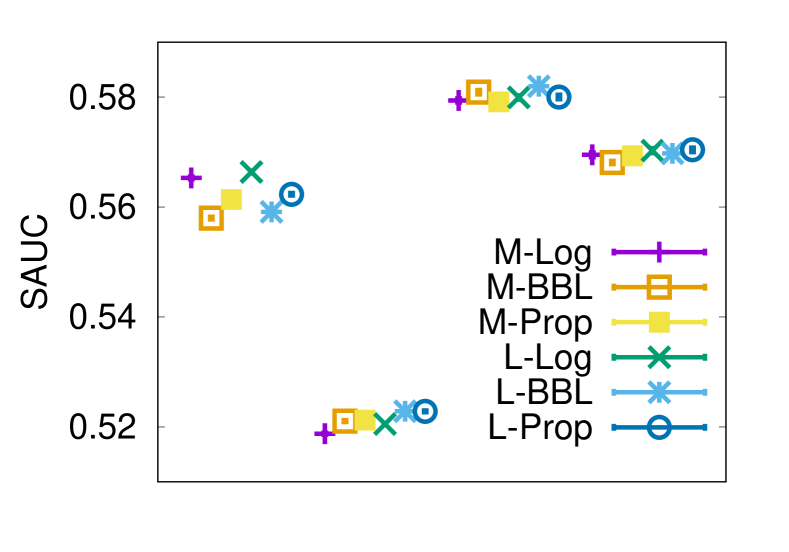
SAUC by MAP estimate or 0.95-UCQE
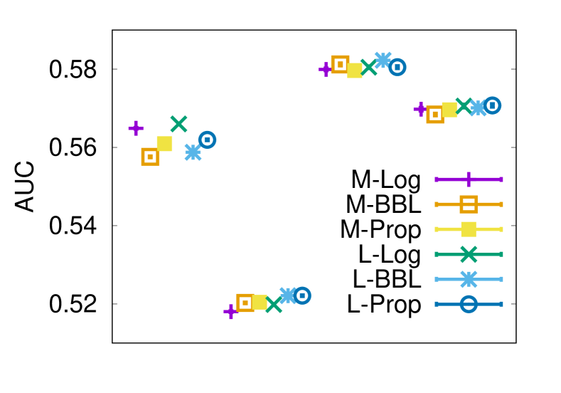
AUC by MAP estimate or 0.95-UCQE
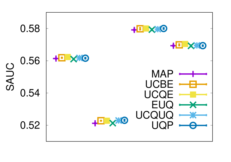
SAUC by various scoring
within the proposed model
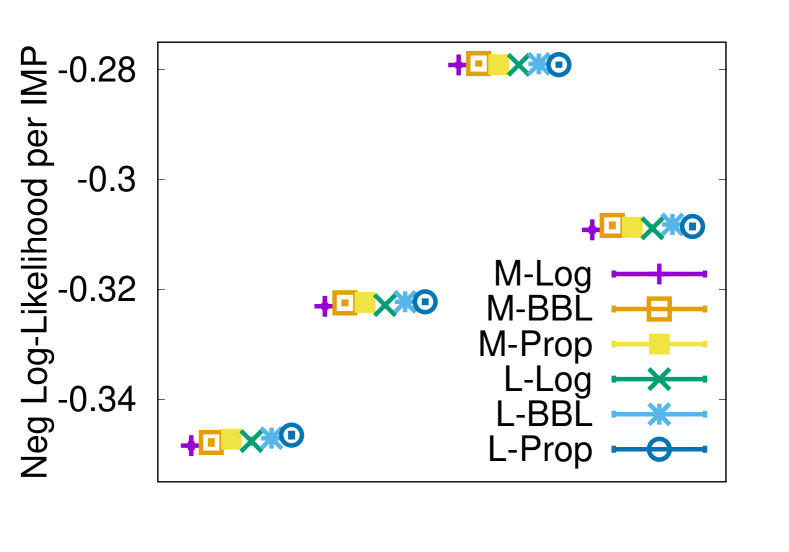
Average log-likelihood
per impression
6 Conclusion
This paper introduced a new contextual Bayesian binary classifier whose risks and/or uncertainties on probabilities of success have been underestimated by existing models. The proposed model consists of a conditional Beta distribution on input vector of context, and its estimation is done with its low-rank Laplace approximation using thin SVD. The closed forms for our approximate posterior yield several uncertainty-aware scoring measures, and parts of them were experimentally successful in early detecting the exceptional articles that are clicked despite the dissimilarity to the positive examples in training period.
In the future, we will apply our philosophy on context-dependent risks and uncertainties for structured non-linear models. We will also qualitatively investigate article examples associated with high uncertainties. We hope our work to become a catalyst for further studies in computational journalism.
References
- [1] W. Chu and S.-T. Park. Personalized recommendation on dynamic content using predictive bilinear models. In Proceedings of the 18th International Conference on World Wide Web (WWW 2009), pages 691–700, New York, NY, USA, 2009. ACM.
- [2] M. Sharma, J. Zhou, J. Hu, and G. Karypis. Feature-based factorized bilinear similarity model for cold-start top-n item recommendation. In Proceedings of the 15th SIAM International Conference on Data Mining (SDM 2015), pages 190–198, 2015.
- [3] Y. Wu, Y. Ding, X. Wang, and J. Xu. Topic based automatic news recommendation using topic model and affinity propagation. In Proceedings of the 27th international conference on Machine Learning and Cybernetics (ICMLC 2010), pages 1299–1304, 2010.
- [4] A. Das, M. Datar, A. Garg, and S. Rajaram. Google news personalization: Scalable online collaborative filtering. In Proceedings of the 16th international conference on World wide web (WWW 2007), pages 271–280, New York, NY, USA, 2010. ACM.
- [5] D. Agarwal and B.-C. Chen. fLDA: Matrix factorization through latent Dirichlet allocation. In Proceedings of the 3rd ACM International Conference on Web Search and Data Mining (WSDM 2010), pages 91–100, New York, NY, USA, 2010. ACM.
- [6] S. Gunasekar, M. Yamada, D. Yin, and Y. Chang. Consistent collective matrix completion under joint low rank structure. In Proceedings of the 18th international conference on Artificial Intelligence and Statistics (AISTATS 2015), volume 38, 2015.
- [7] L. Dali, B. Fortuna, and J. Rupnik. Learning to rank for personalized news article retrieval. In Proceedings of Workshop on Applications of Pattern Analysis (WAPA), pages 152–159, 2010.
- [8] M. Claypool, A. Gokhale, T. Miranda, P. Murnikov, D. Netes, and M. Sartin. Combining content-based and collaborative filters in an online newspaper. In Proceedings of ACM SIGIR Workshop on Recommender Systems, 1999.
- [9] L. Zheng, L. Li, W. Hong, and T. Li. PENETRATE: Personalized news recommendation using ensemble hierarchical clustering. Expert Systems with Applications, 40:2127–2136, 2013.
- [10] Eli Pariser. The Filter Bubble: How the New Personalized Web Is Changing What We Read and How We Think. The Penguin Press, 2011.
- [11] E. Bakshy, S. Messing, and L. Adamic. Exposure to ideologically diverse news and opinion on Facebook. Science 5, 348(6239):1130–1132, 2015.
- [12] Y. Yue and C. Guestrin. Linear submodular bandits and their application to diversified retrieval. In Advances in Neural Information Processing Systems 24, pages 2483–2491. 2011.
- [13] R.H. Affandi, A. Kulesza, and E. Fox. Markov determinantal point processes. In Proceedings of the 28th Conference on Uncertainty in Artificial Intelligence (UAI 2012), 2012.
- [14] J.A. Gillenwater, A. Kulesza, E. Fox, and B. Taskar. Expectation-Maximization for learning determinantal point processes. In Advances in Neural Information Processing Systems 27, pages 3149–3157. 2014.
- [15] Z. Ren and M. de Rijke. Summarizing contrastive themes via hierarchical non-parametric processes. In Proceedings of the 38th International ACM SIGIR Conference on Research and Development in Information Retrieval (SIGIR 2015), pages 93–102, New York, NY, USA, 2015. ACM.
- [16] A. Kulesza and B. Taskar. Determinantal point processes for machine learning. http://arxiv.org/abs/1207.6083, 2013.
- [17] J. Liu, P. Dolan, and E.R. Pedersen. Personalized news recommendation based on click behavior. In Proceedings of the 15th International Conference on Intelligent User Interfaces (IUI 2010), pages 31–40, New York, NY, USA, 2010. ACM.
- [18] L. Li, W. Chu, J. Langford, and R.E. Schapire. A contextual-bandit approach to personalized news article recommendation. In Proceedings of the 19th International Conference on World Wide Web (WWW 2010), pages 661–670, New York, NY, USA, 2010. ACM.
- [19] B.C. May, N. Korda, A. Lee, and D.S. Leslie. Optimistic Bayesian sampling in contextual-bandit problems. Journal of Machine Learning Research, 13:2069–2106, 2012.
- [20] L. Tang, Y. Jiang, L. Li, and T. Li. Ensemble contextual bandits for personalized recommendation. In Proceedings of the 8th ACM Conference on Recommender Systems (RecSys 2014), pages 73–80, 2014.
- [21] S. Rendle. Factorization machines with libFM. ACM Trans. Intell. Syst. Technol., 3(3):57:1–57:22, 2012.
- [22] Y. Juan, Y. Zhuang, W.-S. Chin, and C.-J. Lin. Field-aware factorization machines for CTR prediction. In Proceedings of the 10th ACM Conference on Recommender Systems (RecSys 2016), pages 43–50, 2016.
- [23] P. Covington, J. Adams, and E. Sargin. Deep neural networks for YouTube recommendations. In Proceedings of the 10th ACM Conference on Recommender Systems (RecSys 2016), pages 191–198, 2016.
- [24] E. Contal, V. Perchet, and N. Vayatis. Gaussian process optimization with mutual information. In Proceedings of 31st International Conference on Machine Learning (ICML 2014), 2014.
- [25] H. Tak and C. N. Morris. Data-dependent posterior propriety of a bayesian beta-binomial-logit model. Bayesian Analysis, 12(2):533–555, 2017.
- [26] P. W. Goldberg, C. K. I. Williams, and C. M. Bishop. Regression with input-dependent noise: A Gaussian process treatment. In Proceedings of the 1997 Conference on Advances in Neural Information Processing Systems 10, pages 493–499, Cambridge, MA, USA, 1998. MIT Press.
- [27] C. E. Rasmussen and C. K. I. Williams. Gaussian Processes for Machine Learning (Adaptive Computation and Machine Learning). The MIT Press, 2005.
- [28] T. P. Minka. Expectation propagation for approximate Bayesian inference. In Proceedings of the 17th Conference on Uncertainty in Artificial Intelligence (UAI 2001), pages 362–369, 2001.
- [29] B. Shahbaba and R. Neal. Nonlinear models using Dirichlet process mixtures. Journal of Machine Learning Research, 10:1829–1850, 2009.
- [30] M. Sugiyama, I. Takeuchi, T. Suzuki, T. Kanamori, H. Hachiya, and D. Okanohara. Conditional density estimation via least-squares density ratio estimation. In Proceedings of the 13th International Conference on Artificial Intelligence and Statistics (AISTATS 2010), volume 9, pages 781–788, 2010.
- [31] N. Ding and S.v.n. Vishwanathan. -logistic regression. In Advances in Neural Information Processing Systems 23, pages 514–522. 2010.
- [32] L. R. Pericchi and P. Walley. Robust Bayesian credible intervals and prior ignorance. International Statistical Review / Revue Internationale de Statistique, 59(1):1–23, 1991.
- [33] H. Robbins. Some aspects of the sequential design of experiments. Bulletin of the American Mathematical Society, 58:527–535, 1952.
- [34] D. Kahneman and A. Tversky. Prospect theory: An analysis of decision under risk. Econometrica, 47(2):263–291, 1979.
- [35] M. Usher and J. L. McClelland. Loss aversion and inhibition in dynamical models of multialternative choice. Psychological Review, 111:757–769, 2004.
- [36] E. Higgins. Making a good decision: Value from fit. American Psychologist, 55(11):1217–1230, 2000.
- [37] T. Avnet and E.T. Higgins. How regulatory fit impacts value in consumer choices and opinions. Journal of Marketing Research, 43(1):1–10, 2006.
- [38] P. Frazier, D. Kempe, J. Kleinberg, and R. Kleinberg. Incentivizing exploration. In Proceedings of the 15th ACM Conference on Economics and Computation (EC 2014), pages 5–22. ACM, 2014.
- [39] G.E. Smith, M.P. Venkatraman, and R.R. Dholakia. Diagnosing the search cost effect: Waiting time and the moderating impact of prior category knowledge. Journal of Economic Psychology, 20:285–314, 1999.
- [40] A. Kumar and T. Minakshi. Estimation of variety seeking for segmentation and targeting: An empirical analysis. Journal of Targeting, Measurement and Analysis for Marketing, 15(1):21–29, 2006.
- [41] E. Ho and A. Ilic. Towards high resolution identification of variety seeking behavior. In Proceedings of the 22nd European Conference on Information Systems (ECIS 2014), 2014.
- [42] P.S. Raju. Optimum stimulation level: Its relationship to personality, demographics, and exploratory behavior. Journal of Consumer Research, 7(3):272–282, 1980.
- [43] A. Kulesza and B. Taskar. Learning determinantal point processes. In Proceedings of the 27th Conference on Uncertainty in Artificial Intelligence (UAI 2011), 2011.
- [44] O. Chapelle, E. Manavoglu, and R. Rosales. Simple and scalable response prediction for display advertising. ACM Trans. Intell. Syst. Technol., 5(4):61:1–61:34, 2014.