A randomized Milstein method for
stochastic differential equations with
non-differentiable drift coefficients

Abstract.

In this paper a drift-randomized Milstein method is introduced for the numerical solution of non-autonomous stochastic differential equations with non-differentiable drift coefficient functions. Compared to standard Milstein-type methods we obtain higher order convergence rates in the $L^{p}(\Omega)$ and almost sure sense. An important ingredient in the error analysis are randomized quadrature rules for Hölder continuous stochastic processes. By this we avoid the use of standard arguments based on the Itō-Taylor expansion which are typically applied in error estimates of the classical Milstein method but require additional smoothness of the drift and diffusion coefficient functions. We also discuss the optimality of our convergence rates. Finally, the question of implementation is addressed in a numerical experiment.

1. Introduction

For many decades the numerical solution of stochastic differential equations (SDEs) has been a very active research area in the intersection of probability and numerical analysis. A wide range of applications, for instance, in the engineering and physical sciences as well as in computational finance is still spurring the demand for the development of more efficient algorithms and their theoretical justification. In particular, the current focus lies on the approximation of SDEs which cannot be treated by standard methods found in the pioneering books of P. E. Kloeden and E. Platen [17], or G. N. Milstein and M. V. Tretyakov [24, 25].

Due to the presence of an irregular stochastic forcing term, solutions to SDEs are typically non-smooth. This makes it notoriously difficult to construct higher order numerical approximations. The first successful attempt to construct a first order numerical algorithm for the approximation of an SDE with multiplicative noise led to the well-known Milstein method [22, 23]. Its derivation is based on the Itō-Taylor formula and it can be generalized to construct approximations of, in principle, arbitrary high order provided the coefficient functions are sufficiently smooth. We again refer to the monographs [17, 24, 25].

Unfortunately, the standard smoothness and growth requirements are often not fulfilled in applications. For instance, already in the case of super-linearly growing coefficient functions, the standard Euler-Maruyama and Milstein methods are known to be divergent in the strong and weak sense, see [12]. It is therefore necessary to apply these methods only with caution if the SDE in question does not fit into the framework of [17, 24, 25]. In this paper we focus on the numerical solution of non-autonomous SDEs whose drift coefficient functions are not necessarily differentiable. We will show that a higher order approximation of the exact solution that outperforms the Euler-Maruyama method can still be obtained in this case by using suitable Monte Carlo randomization techniques.

To be more precise, let $T\in(0,\infty)$ and $(\Omega_{W},{\mathcal{F}}^{W},({\mathcal{F}}^{W}_{t})_{t\in[0,T]},{\mathbb{P}}_{W})$ be a filtered probability space satisfying the usual conditions. For $d,m\in{\mathbb{N}}$ let $W\colon[0,T]\times\Omega_{W}\to{\mathbb{R}}^{m}$ be a standard $({\mathcal{F}}^{W}_{t})_{t\in[0,T]}$-Wiener process. Moreover, let $X\colon[0,T]\times\Omega_{W}\to{\mathbb{R}}^{d}$ be an $({\mathcal{F}}^{W}_{t})_{t\in[0,T]}$-adapted stochastic process that is a solution to the Itō-type stochastic differential equation

(1) $$\begin{split}\begin{cases}\,\mathrm{d}X(t)&=f(t,X(t))\,\mathrm{d}t+\sum_{r=1}^{m}g^{r}\big{(}t,X(t)\big{)}\,\mathrm{d}W^{r}(t),\quad t\in[0,T],\\ X(0)&=X_{0},\end{cases}\end{split}$$

where $X_{0}\in L^{2p}(\Omega_{W},{\mathcal{F}}^{W}_{0},{\mathbb{P}}_{W};{\mathbb{R}}^{d})$ for some $p\in[2,\infty)$ denotes the initial value. The drift coefficient function $f\colon[0,T]\times{\mathbb{R}}^{d}\to{\mathbb{R}}^{d}$ and the diffusion coefficient functions $g^{r}\colon[0,T]\times{\mathbb{R}}^{d}\to{\mathbb{R}}^{d}$ for $r\in\{1,2,\ldots,m\}$ are assumed to satisfy certain Lipschitz and linear growth conditions. For a complete statement of all conditions on $f$ and $g^{r}$ we refer to Section 3.

If the drift function $f$ is only $\gamma$-Hölder continuous, $\gamma\in(0,1]$, with respect to the time variable and Lipschitz continuous with respect to the state variable (see Assumption 3.2), then it is well-known that in the deterministic case ($g^{r}\equiv 0$ for all $r\in\{1,\ldots,m\}$) the order of convergence of the standard Euler method can, in general, not exceed $\gamma$. This is even true for any deterministic algorithm that only uses finitely many point evaluations of the drift $f$, see [11, 14].

One possibility to increase the order of convergence in such a case consists of a suitable combination of the one-step method with certain Monte-Carlo techniques. For deterministic differential equations this has been studied, for example, in [4, 11, 13, 15, 20, 33, 34]. In particular, in [4, 11, 20] certain randomized Euler and Runge-Kutta methods are introduced which converge with order $\gamma+\frac{1}{2}$ under the same smoothness assumptions on $f$ as above. In fact, these convergence rates are shown to be optimal within the class of all randomized algorithms, see [11].

The purpose of this paper is to combine these randomization techniques with the classical Milstein scheme in order to obtain a higher order approximation method in the case of a non-differentiable drift coefficient function $f$. For the introduction of the resulting drift-randomized Milstein method let $\pi_{h}$ be a not necessarily equidistant temporal grid of the form

(2) $$\pi_{h}:=\{t_{j}\;:\;j=0,1,\ldots,N_{h},\;0=t_{0}<t_{1}<\ldots<t_{N_{h}-1}<t_{N_{h}}=T\},$$

where $N_{h}\in{\mathbb{N}}$ and $h_{j}:=t_{j}-t_{j-1}$ is the width of the $j$-th step. Given a temporal grid $\pi_{h}$ we denote the associated vector of all step sizes by

(3) $$h:=(h_{j})_{j=1}^{N_{h}}\in{\mathbb{R}}^{N_{h}}\quad\text{ with }t_{n}=\sum_{j=1}^{n}h_{j}.$$

The maximum step size in $\pi_{h}$ is then denoted by

$$|h|:=\max_{j\in\{1,\ldots,N_{h}\}}h_{j}.$$

Further, let $(\tau_{j})_{j\in{\mathbb{N}}}$ be an i.i.d. family of $\mathcal{U}(0,1)$-distributed random variables on an additional filtered probability space $(\Omega_{\tau},{\mathcal{F}}^{\tau},({\mathcal{F}}^{\tau}_{j})_{j\in{\mathbb{N}}},{\mathbb{P}}_{\tau})$, where ${\mathcal{F}}_{j}^{\tau}$ is the $\sigma$-algebra generated by $\{\tau_{1},\ldots,\tau_{j}\}$. The random variables $(\tau_{j})_{j\in{\mathbb{N}}}$ represent the artificially added random input for the new method, which we assume to be independent of the randomness already present in SDE (1).

The resulting numerical method will then yield a discrete-time stochastic process defined on the product probability space

(4) $$(\Omega,{\mathcal{F}},{\mathbb{P}}):=(\Omega_{W}\times\Omega_{\tau},{\mathcal{F}}^{W}\otimes{\mathcal{F}}^{\tau},{\mathbb{P}}_{W}\otimes{\mathbb{P}}_{\tau}).$$

Moreover, for each temporal grid $\pi_{h}$ a discrete-time filtration $({\mathcal{F}}^{h}_{n})_{n\in\{1,\ldots,N_{h}\}}$ on $(\Omega,{\mathcal{F}},{\mathbb{P}})$ is given by

(5) $${\mathcal{F}}^{h}_{n}:={\mathcal{F}}^{W}_{t_{n}}\otimes{\mathcal{F}}^{\tau}_{n},\quad\text{ for }n\in\{0,1,\ldots,N_{h}\}.$$

Finally, for the formulation of the drift-randomized Milstein method, we also recall the following standard notation for the stochastic increments and iterated stochastic integrals (c.f.[17, 24, 25]): For $s,t\in[0,T]$ with $s<t$ set

(6) $$I_{(r)}^{s,t} :=\int_{s}^{t}\,\mathrm{d}W^{r}(u),\ \ \ \mbox{for \ }r\in\{1,2,\ldots,m\},$$

(7) $$I_{(r_{1},r_{2})}^{s,t} :=\int_{s}^{t}\int_{s}^{u_{1}}\,\mathrm{d}W^{r_{1}}(u_{2})\,\mathrm{d}W^{r_{2}}(u_{1}),\ \ \ \mbox{for\ }r_{1},r_{2}\in\{1,2,\ldots,m\}.$$

We further introduce the mapping $g^{r_{1},r_{2}}\colon[0,T]\times{\mathbb{R}}^{d}\to{\mathbb{R}}^{d}$ given by

(8) $$g^{r_{1},r_{2}}(t,x):=\frac{\partial g^{r_{1}}}{\partial x}(t,x)g^{r_{2}}(t,x),$$

for all $r_{1},r_{2}\in\{1,2,\ldots,m\}$, $t\in[0,T]$, $x\in{\mathbb{R}}^{d}$. Then, the drift-randomized Milstein method on the grid $\pi_{h}$ is given by the split-step recursion

(9) $$\begin{split}X_{h}^{j,\tau}=&X_{h}^{j-1}+\tau_{j}h_{j}f\big{(}t_{j-1},X_{h}^{j-1}\big{)}+\sum_{r=1}^{m}g^{r}\big{(}t_{j-1},X_{h}^{j-1}\big{)}I^{t_{j-1},t_{j-1}+\tau_{j}h_{j}}_{(r)},\\ X_{h}^{j}=&X_{h}^{j-1}+h_{j}f(t_{j-1}+\tau_{j}h_{j},X_{h}^{j,\tau})+\sum_{r=1}^{m}g^{r}(t_{j-1},X_{h}^{j-1})I^{t_{j-1},t_{j}}_{(r)}\\ &+\sum_{r_{1},r_{2}=1}^{m}g^{r_{1},r_{2}}(t_{j-1},X_{h}^{j-1})I_{(r_{2},r_{1})}^{t_{j-1},t_{j}},\end{split}$$

for all $j\in\{1,\ldots,N_{h}\}$, and the initial value $X_{h}^{0}=X_{0}$.

The main result of this paper then shows that this method converges to the exact solution with respect to the norm in $L^{p}(\Omega)$, $p\in[2,\infty)$. More precisely, Theorem 3.8 states that under Assumptions 3.1 to 3.3 there exists $C\in(0,\infty)$ independent of the temporal grid $\pi_{h}$ such that

$$\big{\|}\max_{n\in\{0,1,\ldots,N_{h}\}}|X_{h}^{n}-X(t_{n})|\big{\|}_{L^{p}(\Omega)}\leq C|h|^{\min(\frac{1}{2}+\gamma,1)},$$

where $\gamma\in(0,1]$ denotes as above the temporal Hölder regularity of the drift coefficient function. It turns out that this convergence rate is optimal under these conditions on $f$ as we will discuss in more detail in Section 3. In addition, it is a simple consequence of Theorem 3.8 that the drift-randomized Milstein method is then also convergent in a pathwise sense, see Corollary 3.9.

In Section 7 we will also illustrate that the randomized Milstein method is easily implemented for a scalar noise. For a multi-dimensional Wiener process the joint simulation of the iterated stochastic integrals (7) is, in general, very costly. Since this issue also applies to the classical Milstein it is, however, not further addressed in this paper. Instead we refer to the discussion in [17, Chap. 5]. Further approximation methods for the simulation of iterated stochastic integrals are found, for instance, in [6, 30, 36]. Moreover, it is worth mentioning that, besides the case of commutative noise (see [17, Chap. 10.3]), the simulation of the iterated stochastic integrals (7) can also be avoided if the Milstein method is combined with an antithetic multilevel Monte Carlo algorithm, see [7].

Before we give an outline of the remainder of this paper, let us briefly mention that drift-randomized one-step methods for the numerical solution of SDEs have also been studied by P. Przybyłowicz and P. Morkisz [26, 27, 28, 29]. Here the focus lies on randomized Euler-Maruyama type methods applied to SDEs, whose drift-coefficient functions are of Carathéodory-type. In particular, the authors derive optimal and minimal error estimates in the case of drift coefficient functions, that are discontinuous with respect to the temporal argument $t$.

In the following sections we will first focus on the error analysis of the drift-randomized Milstein method. To this end we fix further notation and recall some useful results from stochastic analysis in Section 2. In Section 3 we then formulate the main result on the convergence of the drift-randomized Milstein method in the $L^{p}(\Omega)$ and almost sure sense. In addition, this section also includes a complete list of all imposed conditions on the drift and diffusion coefficient functions and some properties of the exact solution to (1). For the proof of our main result stated in Theorem 3.8 we then employ a framework developed in [1]. For this we first prove in Section 5 that the method (9) is stochastically bistable. The second ingredient in the error analysis is then to show that the method is also consistent. This will be done in Section 6. Our proof of consistency is based on some error estimates for randomized quadrature rules applied to stochastic processes. This result of possibly independent interest generalizes error estimates for Monte Carlo integration from [9, 10] and is presented in Section 4. Finally, in Section 7 we illustrate the practicability of the drift-randomized Milstein method through a numerical experiment.

2. Notation and preliminaries

In this section we explain the notation that is used throughout this paper. In addition, we also collect a few standard results from stochastic analysis, which are needed in later sections.

By ${\mathbb{N}}$ we denote the set of all positive integers, while ${\mathbb{N}}_{0}:={\mathbb{N}}\cup\{0\}$. As usual the set ${\mathbb{R}}$ consists of all real numbers. By $|\cdot|$ we denote the Euclidean norm on the Euclidean space ${\mathbb{R}}^{d}$ for any $d\in{\mathbb{N}}$. In particular, if $d=1$ then $|\cdot|$ coincides with taking the absolute value. Moreover, the norm $|\cdot|_{\mathcal{L}({\mathbb{R}}^{d})}$ denotes the standard matrix norm on ${\mathbb{R}}^{d\times d}$ induced by the Euclidean norm.

We will also frequently encounter normed function spaces. First, for an arbitrary Banach space $(E,\|\cdot\|_{E})$ we denote by $\mathcal{C}^{\gamma}([0,T];E)$ with $T\in(0,\infty)$ and $\gamma\in(0,1]$ the space of all $\gamma$-Hölder continuous $E$-valued mappings $v\colon[0,T]\to E$ with norm

$$\|v\|_{\mathcal{C}^{\gamma}([0,T];E)}=\sup_{t\in[0,T]}\|v(t)\|_{E}+\sup_{\begin{subarray}{c}t,s\in[0,T]\\ t\neq s\end{subarray}}\frac{\|v(t)-v(s)\|_{E}}{|t-s|^{\gamma}}.$$

For a given measure space $(X,\mathcal{A},\mu)$ the set $L^{p}(X;E):=L^{p}(X,\mathcal{A},\mu;E)$, $p\in[1,\infty)$, consists of all (equivalence classes of) Bochner measurable functions $v\colon X\to E$ with

$$\|v\|_{L^{p}(X;E)}:=\Big{(}\int_{X}\|v(x)\|_{E}^{p}\,\mathrm{d}\mu(x)\Big{)}^{\frac{1}{p}}<\infty.$$

If $(E,\|\cdot\|_{E})=({\mathbb{R}},|\cdot|)$ we use the abbreviation $L^{p}(X):=L^{p}(X;{\mathbb{R}})$. If $(X,\mathcal{A},\mu)=(\Omega,{\mathcal{F}},{\mathbb{P}})$ is a probability space, we usually write the integral with respect to the probability measure ${\mathbb{P}}$ as

$${\mathbb{E}}[Z]:=\int_{\Omega}Z(\omega)\,\mathrm{d}{\mathbb{P}}(\omega),\quad Z\in L^{p}(\Omega;E).$$

In the case of the product probability space $(\Omega,{\mathcal{F}},{\mathbb{P}})$ introduced in (4) an application of Fubini’s theorem shows that

$${\mathbb{E}}[Z]={\mathbb{E}}_{W}[{\mathbb{E}}_{\tau}[Z]]={\mathbb{E}}_{\tau}[{\mathbb{E}}_{W}[Z]],\quad Z\in L^{p}(\Omega;E),$$

where ${\mathbb{E}}_{W}$ is the expectation with respect to ${\mathbb{P}}_{W}$ and ${\mathbb{E}}_{\tau}$ with respect to ${\mathbb{P}}_{\tau}$. Finally, $\mathcal{U}(0,1)$ denotes the uniform distribution on the interval $(0,1)$.

An important tool is the following discrete-time version of the Burkholder-Davis-Gundy inequality from [2].

Theorem 2.1.

For each $p\in(1,\infty)$ there exist positive constants $c_{p}$ and $C_{p}$ such that for every discrete-time martingale $(Y^{n})_{n\in{\mathbb{N}}_{0}}$ and for every $n\in{\mathbb{N}}_{0}$ we have

$$c_{p}\big{\|}[Y]_{n}^{\frac{1}{2}}\big{\|}_{L^{p}(\Omega)}\leq\big{\|}\max_{j\in\{0,\ldots,n\}}|Y^{j}|\big{\|}_{L^{p}(\Omega)}\leq C_{p}\big{\|}[Y]_{n}^{\frac{1}{2}}\big{\|}_{L^{p}(\Omega)},$$

where $[Y]_{n}=|Y^{0}|^{2}+\sum_{k=1}^{n}|Y^{k}-Y^{k-1}|^{2}$ is the quadratic variation of $(Y^{n})_{n\in{\mathbb{N}}_{0}}$.

The following theorem contains a useful estimate of stochastic Itō-integrals with respect to the $L^{p}(\Omega;{\mathbb{R}}^{d})$-norm. For a proof we refer to [21, Section 1.7].

Theorem 2.2.

Let $W\colon[0,T]\times\Omega_{W}\to{\mathbb{R}}$ be a standard $({\mathcal{F}}_{t}^{W})_{t\in[0,T]}$-Wiener process on $(\Omega_{W},{\mathcal{F}}^{W},{\mathbb{P}}^{W})$. Let $Y\colon[0,T]\times\Omega_{W}\to{\mathbb{R}}^{d}$ be a stochastically integrable, $({\mathcal{F}}_{t}^{W})_{t\in[0,T]}$-adapted process with $Y\in L^{p}([0,T]\times\Omega_{W};{\mathbb{R}}^{d})$ for some $p\in[2,\infty)$. Then, for all $t,s\in[0,T]$ with $s<t$, it holds true that

$$\Big{\|}\int_{s}^{t}Y(u)\,\mathrm{d}W(u)\Big{\|}_{L^{p}(\Omega_{W};{\mathbb{R}}^{d})}\leq C_{p}(t-s)^{\frac{p-2}{2p}}\|Y\|_{L^{p}([s,t]\times\Omega_{W};{\mathbb{R}}^{d})}$$

with $C_{p}=(\frac{1}{2}p(p-1))^{\frac{1}{2}}$.

The next inequality is a useful tool to bound the error of a numerical approximation. For a proof we refer, for instance, to [5, Proposition 4.1].

Lemma 2.3 (Discrete Gronwall’s inequality).

Consider two nonnegative sequences $(u_{n})_{n\in{\mathbb{N}}},(w_{n})_{n\in{\mathbb{N}}}\subset{\mathbb{R}}$ which for some given $a\in[0,\infty)$ satisfy

$$u_{n}\leq a+\sum_{j=1}^{n-1}w_{j}u_{j},\quad\text{ for all }n\in{\mathbb{N}}.$$

Then, for all $n\in{\mathbb{N}}$, it also holds true that $u_{n}\leq a\exp(\sum_{j=1}^{n-1}w_{j}).$

3. Assumptions and main results

In this section we present sufficient conditions for the convergence of the drift-randomized Milstein method (9) with respect to the norm in $L^{p}(\Omega)$ for some $p\in[2,\infty)$. After collecting a few important properties of the exact solution, we state and discuss the main results of this paper, namely the convergence of the method in the $L^{p}(\Omega)$-norm and in the almost sure sense.

Assumption 3.1.

There exists $p\in[2,\infty)$ such that the initial value satisfies $X_{0}\in L^{2p}(\Omega_{W},{\mathcal{F}}_{0}^{W},{\mathbb{P}}_{W};{\mathbb{R}}^{d})$.

Assumption 3.2.

The drift coefficient function $f\colon[0,T]\times{\mathbb{R}}^{d}\to{\mathbb{R}}^{d}$ is assumed to be continuous. Moreover, there exist $\gamma\in(0,1]$ and $K_{f}\in(0,\infty)$ such that

$$|f(t,x_{1})-f(t,x_{2})| \leq K_{f}|x_{1}-x_{2}|,$$

$$|f(t_{1},x)-f(t_{2},x)| \leq K_{f}(1+|x|)|t_{1}-t_{2}|^{\gamma},$$

for all $t,t_{1},t_{2}\in[0,T]$, $x,x_{1},x_{2}\in{\mathbb{R}}^{d}$.

For the formulation of Assumption 3.3 recall the definition of $g^{r_{1},r_{2}}$ from (8).

Assumption 3.3.

The diffusion coefficient functions $g^{r}\colon[0,T]\times{\mathbb{R}}^{d}\to{\mathbb{R}}^{d}$, $r\in\{1,\ldots,m\}$, are assumed to be continuous. In addition, we assume that for every fixed $t\in[0,T]$ and $r\in\{1,\ldots,m\}$ the mapping ${\mathbb{R}}^{d}\ni x\mapsto g^{r}(t,x)\in{\mathbb{R}}^{d}$ is continuously differentiable. Moreover, there exist $\gamma\in(0,1]$ and $K_{g}\in(0,\infty)$ with

$$|g^{r}(t_{1},x)-g^{r}(t_{2},x)| \leq K_{g}(1+|x|)|t_{1}-t_{2}|^{\min(\frac{1}{2}+\gamma,1)},$$

$$\Big{|}\frac{\partial g^{r}}{\partial x}(t,x_{1})-\frac{\partial g^{r}}{\partial x}(t,x_{2})\Big{|}_{\mathcal{L}({\mathbb{R}}^{d})} \leq K_{g}|x_{1}-x_{2}|,$$

$$\Big{|}\frac{\partial g^{r}}{\partial x}(t,x)\Big{|}_{\mathcal{L}({\mathbb{R}}^{d})} \leq K_{g},$$

$$\big{|}g^{r_{1},r_{2}}(t,x_{1})-g^{r_{1},r_{2}}(t,x_{2})\big{|} \leq K_{g}|x_{1}-x_{2}|$$

for all $t_{1},t_{2}\in[0,T]$ and $x\in{\mathbb{R}}^{d}$ and $r,r_{1},r_{2}\in\{1,2,\ldots,m\}$.

Remark 3.4.

(i) It directly follows from Assumption 3.2 that $f$ satisfies a linear growth bound for all $t\in[0,T]$ and $x\in{\mathbb{R}}^{d}$ of the form

(10) $$|f(t,x)|\leq\tilde{K}_{f}\big{(}1+|x|\big{)}$$

with $K_{f}\leq\tilde{K}_{f}=\max(K_{f},T^{\gamma}K_{f}+|f(0,0)|)$.

(ii) The boundedness of $\frac{\partial g^{r}}{\partial x}$ immediately implies that $g^{r}$, $r=1,\ldots,m$, is globally Lipschitz continuous. More precisely, for all $t\in[0,T]$ and $x_{1},x_{2}\in{\mathbb{R}}^{d}$ we have

(11) $$|g^{r}(t,x_{1})-g^{r}(t,x_{2})| \leq K_{g}|x_{1}-x_{2}|.$$

Together with the temporal Hölder continuity of $g^{r}$ this also implies a linear growth bound of the form

(12) $$|g^{r}(t,x)|\leq\tilde{K}_{g}\big{(}1+|x|\big{)}$$

with $K_{g}\leq\tilde{K}_{g}=\max(K_{g},T^{\min(\frac{1}{2}+\gamma,1)}K_{g}+\max_{r\in\{1,\ldots,m\}}|g^{r}(0,0)|)$.

Before moving to the main result, let us collect a few useful properties of the exact solution $X$ to the SDE (1). A proof is found, e.g., in [21, Sect. 2.3, 2.4].

Theorem 3.5.

Let Assumptions 3.1 to 3.3 be satisfied with $p\in[2,\infty)$. Then there exists an up to indistinguishability uniquely determined $({\mathcal{F}}_{t}^{W})_{t\in[0,T]}$-adapted stochastic process $X\colon[0,T]\times\Omega\to{\mathbb{R}}^{d}$ satisfying (1). More precisely, for every $t\in[0,T]$ it holds true that

(13) $$X(t)=X_{0}+\int_{0}^{t}f(s,X(s))\,\mathrm{d}s+\sum_{r=1}^{m}\int_{0}^{t}g^{r}(s,X(s))\,\mathrm{d}W^{r}(s)$$

with probability one. Moreover, there exists $C\in(0,\infty)$ only depending on $\tilde{K}_{f}$, $\tilde{K}_{g}$, $p$, and $T$ such that

(14) $$\big{\|}\sup_{t\in[0,T]}|X(t)|\big{\|}_{L^{2p}(\Omega_{W})}\leq C\big{(}1+\big{\|}X_{0}\big{\|}_{L^{2p}(\Omega_{W};{\mathbb{R}}^{d})}\big{)}.$$

In addition, for all $s,t\in[0,T]$ we have

(15) $$\big{\|}X(t)-X(s)\big{\|}_{L^{2p}(\Omega_{W};{\mathbb{R}}^{d})}\leq C\big{(}1+\big{\|}X_{0}\big{\|}_{L^{2p}(\Omega_{W};{\mathbb{R}}^{d})}\big{)}|t-s|^{\frac{1}{2}}.$$

In particular, it holds $X\in\mathcal{C}^{\frac{1}{2}}([0,T],L^{2p}(\Omega_{W};{\mathbb{R}}^{d}))$ with

$$\|X\|_{\mathcal{C}^{\frac{1}{2}}([0,T],L^{2p}(\Omega_{W};{\mathbb{R}}^{d}))}\leq C\big{(}1+\big{\|}X_{0}\big{\|}_{L^{2p}(\Omega_{W};{\mathbb{R}}^{d})}\big{)}.$$

Let us now turn to the drift-randomized Milstein method (9). In the following it is convenient to formally introduce the increment function of the numerical method. For this let $\pi_{h}$ be an arbitrary temporal grid as in (2). Then for each $j\in\{1,\ldots,N_{h}\}$ the increment function $\Phi^{j}_{h}\colon{\mathbb{R}}^{d}\times[0,1]\times\Omega_{W}\to{\mathbb{R}}^{d}$ of the $j$-th step is defined by

(16) $$\begin{split}\Phi^{j}_{h}(y,\tau)&:=h_{j}f(t_{j-1}+\tau h_{j},\Psi_{h}^{j}(y,\tau))+\sum_{r=1}^{m}g^{r}(t_{j-1},y)I^{t_{j-1},t_{j}}_{(r)}\\ &\qquad+\sum_{r_{1},r_{2}=1}^{m}g^{r_{1},r_{2}}(t_{j-1},y)I_{(r_{2},r_{1})}^{t_{j-1},t_{j}},\end{split}$$

for all $y\in{\mathbb{R}}^{d}$ and $\tau\in[0,1]$, where

(17) $$\Psi_{h}^{j}(y,\tau):=y+\tau h_{j}f\big{(}t_{j-1},y\big{)}+\sum_{r=1}^{m}g^{r}\big{(}t_{j-1},y\big{)}I^{t_{j-1},t_{j-1}+\tau h_{j}}_{(r)}.$$

In terms of $\Phi_{h}$ we can then rewrite the recursion defining the method (9) by

(18) $$\begin{cases}X_{h}^{j}=X_{h}^{j-1}+\Phi^{j}_{h}(X_{h}^{j-1},\tau_{j}),&\quad j\in\{1,\ldots,N_{h}\},\\ X_{h}^{0}=X_{0}.&\end{cases}$$

The next lemma ensures that (18) indeed admits an adapted sequence in $L^{p}(\Omega;{\mathbb{R}}^{d})$.

Lemma 3.6.

Let Assumptions 3.2 and 3.3 be satisfied. Let $\pi_{h}$ be an arbitrary temporal grid and $j\in\{1,\ldots,N_{h}\}$. For every $Z\in L^{p}(\Omega,{\mathcal{F}}^{h}_{j-1},{\mathbb{P}};{\mathbb{R}}^{d})$, $p\in[2,\infty)$, it then holds true that

(19) $$\Phi_{h}^{j}(Z,\tau_{j})\in L^{p}(\Omega,{\mathcal{F}}^{h}_{j},{\mathbb{P}};{\mathbb{R}}^{d}).$$

Proof.

From the continuity of $f$, $g^{r}$, and $g^{r_{1},r_{2}}$ it follows that $\Phi_{h}^{j}(Z,\tau_{j})\colon\Omega\to{\mathbb{R}}^{d}$ is ${\mathcal{F}}^{h}_{j}$-measurable. Hence, it remains to prove the $L^{p}$ boundedness of $\Phi_{h}^{j}(Z,\tau_{j})$. As in (16) we split $\Phi_{h}$ into three terms

$$\Phi^{j}_{h}(Z,\tau_{j})=:\Pi^{j}_{1}+\Pi_{2}^{j}+\Pi_{3}^{j}.$$

We give estimates for these terms separately. First, for the estimate of $\Pi_{2}^{j}$ we have

$$\|\Pi^{j}_{2}\|_{L^{p}(\Omega;{\mathbb{R}}^{d})} =\Big{\|}\sum_{r=1}^{m}g^{r}(t_{j-1},Z)I_{(r)}^{t_{j-1},t_{j}}\Big{\|}_{L^{p}(\Omega;{\mathbb{R}}^{d})}$$

$$\leq\sum_{r=1}^{m}\big{\|}g^{r}(t_{j-1},Z)\big{\|}_{L^{p}(\Omega;{\mathbb{R}}^{d})}\|I_{(r)}^{t_{j-1},t_{j}}\big{\|}_{L^{p}(\Omega)}$$

$$\leq mC_{p}\tilde{K}_{g}\big{(}1+\|Z\|_{L^{p}(\Omega;{\mathbb{R}}^{d})}\big{)}h_{j}^{\frac{1}{2}}<\infty,$$

where the penultimate line is deduced from the triangle inequality and the independence of $Z$ and the increment of the Brownian motion $I_{(r)}^{t_{j-1},t_{j}}$. In addition, the last line follows from the linear growth (12) of $g$ and Theorem 2.2 applied to the stochastic increment.

The estimate of $\Pi_{3}^{j}:=\sum_{r_{1},r_{2}=1}^{m}g^{r_{1},r_{2}}(t_{j-1},Z)I_{(r_{2},r_{1})}^{t_{j-1},t_{j}}$ is obtained similarly by

$$\|\Pi^{j}_{3}\|_{L^{p}(\Omega;{\mathbb{R}}^{d})} \leq\sum_{r_{1},r_{2}=1}^{m}\big{\|}g^{r_{1},r_{2}}(t_{j-1},Z)\big{\|}_{L^{p}(\Omega;{\mathbb{R}}^{d})}\big{\|}I_{(r_{2},r_{1})}^{t_{j-1},t_{j}}\big{\|}_{L^{p}(\Omega)}$$

$$\leq m^{2}C_{p}^{2}K_{g}\tilde{K}_{g}\big{(}1+\|Z\|_{L^{p}(\Omega;{\mathbb{R}}^{d})}\big{)}h_{j}<\infty,$$

where the last line is deduced from the linear growth of $g^{r_{2}}$ and the boundedness of the derivative of $g^{r_{1}}$. In addition, by Theorem 2.2 it holds true that

(20) $$\big{\|}I^{t_{j-1},t_{j}}_{(r_{2},r_{1})}\big{\|}_{L^{p}(\Omega)} \leq C_{p}^{2}h_{j}$$

for all $r_{1},r_{2}\in\{1,\ldots,m\}$ with the same constant $C_{p}$ as above.

It remains to show the $L^{p}$-estimate of $\Pi_{1}^{j}:=h_{j}f\big{(}t_{j-1}+\tau_{j}h_{j},\Psi_{h}^{j}(Z,\tau_{j})\big{)}$. The linear growth (10) of $f$ implies

$$\|\Pi^{j}_{3}\|_{L^{p}(\Omega;{\mathbb{R}}^{d})}\leq\tilde{K}_{f}\big{(}1+\|\Psi_{h}^{j}(Z,\tau_{j})\|_{L^{p}(\Omega;{\mathbb{R}}^{d})}\big{)}h_{j},$$

where $\Psi_{h}$, defined in (17), can be further estimated through the linear growth of both $f$ and $g^{r}$ as well as Theorem 2.2:

$$\|\Psi_{h}^{j}(Z,\tau_{j})\|_{L^{p}(\Omega;{\mathbb{R}}^{d})} \leq\|Z\|_{L^{p}(\Omega;{\mathbb{R}}^{d})}+h_{j}\|f(t_{j-1},Z)\|_{L^{p}(\Omega;{\mathbb{R}}^{d})}$$

$$\quad+\sum_{r=1}^{m}\big{\|}g^{r}(t_{j-1},Z)\big{\|}_{L^{p}(\Omega;{\mathbb{R}}^{d})}\|I_{(r)}^{t_{j-1},t_{j-1}+\tau_{j}h_{j}}\big{\|}_{L^{p}(\Omega)}$$

$$\leq\|Z\|_{L^{p}(\Omega;{\mathbb{R}}^{d})}+\big{(}1+\|Z\|_{L^{p}(\Omega;{\mathbb{R}}^{d})}\big{)}(\tilde{K}_{f}h_{j}+mC_{p}\tilde{K}_{g}h_{j}^{\frac{1}{2}})<\infty.$$

Here the estimate of the increment $I_{(r)}^{t_{j-1},t_{j-1}+\tau_{j}h_{j}}$ comes from

(21) $$\begin{split}\big{\|}I^{t_{j-1},t_{j-1}+\tau_{j}h_{j}}_{(r)}\big{\|}_{L^{p}(\Omega)}&=\big{\|}W^{r}(t_{j-1}+\tau_{j}h_{j})-W^{r}(t_{j-1})\big{\|}_{L^{p}(\Omega)}\\ &=\big{(}{\mathbb{E}}_{\tau}\big{[}{\mathbb{E}}_{W}[|W^{r}(t_{j-1}+\tau_{j}h_{j})-W^{r}(t_{j-1})|^{p}]\big{]}\big{)}^{\frac{1}{p}}\\ &\leq\Big{(}\frac{p(p-1)}{2}\Big{)}^{\frac{1}{2}}h_{j}^{\frac{1}{2}}\big{(}{\mathbb{E}}_{\tau}\big{[}\tau_{j}^{\frac{p}{2}}\big{]}\big{)}^{\frac{1}{p}}\leq C_{p}h_{j}^{\frac{1}{2}}\end{split}$$

by an application of Theorem 2.2. ∎

Definition 3.7.

We say that the numerical method (9) converges with order $\beta\in(0,\infty)$ to the exact solution $X$ of (1) in the $L^{p}(\Omega)$-norm if there exist $p\in[2,\infty)$, $C\in(0,\infty)$, $h_{0}\in(0,T)$ such that for all temporal grids $\pi_{h}$ with $|h|\leq h_{0}$ we have

$$\big{\|}\max_{n\in\{0,1,\ldots,N_{h}\}}|X_{h}^{n}-X(t_{n})|\big{\|}_{L^{p}(\Omega)}\leq C|h|^{\beta}.$$

Here $(X_{h}^{n})_{n\in\{0,1,\ldots,N_{h}\}}\subset L^{p}(\Omega;{\mathbb{R}}^{d})$ is generated by (9) on $\pi_{h}$.

Next, we state our main result. The proof is deferred to the end of Section 6.

Theorem 3.8.

Let Assumptions 3.1 to 3.3 be satisfied with $p\in[2,\infty)$ and $\gamma\in(0,1]$. Then, the drift-randomized Milstein method (9) converges with order $\beta=\min(\frac{1}{2}+\gamma,1)$ to the exact solution $X$ of (1) in the $L^{p}(\Omega)$-norm.

We remark that the order of convergence $\min(\frac{1}{2}+\gamma,1)$ is optimal in the following sense: First, recall that the maximum order of convergence of the classical Milstein method is known to be $1$. This has been shown in [18, Thm. 6.2] by a generalization of the well-known example of Clark and Cameron [3]. Since that example does not contain a drift coefficient function, the classical Milstein method and our randomized version (9) coincide in this case. Therefore, the maximum order of convergence of (9) cannot exceed $1$ as well.

Second, as already mentioned in Section 1, in the ODE case ($g^{r}\equiv 0$ for all $r\in\{1,\ldots,m\}$) the maximum order of convergence of randomized algorithms is known to be equal to $\frac{1}{2}+\gamma$ under Assumption 3.2, see [11]. In addition, it is shown in [29] that the maximum order of convergence for the approximation of a stochastic integral with $(\frac{1}{2}+\gamma)$-Hölder continuous integrand can also not exceed $\frac{1}{2}+\gamma$. Therefore, there exists no (randomized) algorithm, depending only on finitely many point evaluations of the coefficients, that converges with a better rate than $\beta=\min(\frac{1}{2}+\gamma,1)$ for all $f$ and $g^{r}$ satisfying Assumptions 3.2 and 3.3.

We conclude this section with the following convergence result in the almost sure sense. Its proof follows directly from Theorem 3.8 and a modified version of [16, Lemma 2.1] found in [20, Lemma 3.3]. Compare further with [8].

Corollary 3.9.

Let Assumptions 3.1 to 3.3 be satisfied with $p\in[2,\infty)$ and $\gamma\in(0,1]$. Let $(\pi_{h^{(m)}})_{m\in{\mathbb{N}}}\subset[0,T]$ be a sequence of temporal grids with corresponding maximum step sizes $|h^{(m)}|$ satisfying $\sum_{m=1}^{\infty}|h^{(m)}|<\infty$. Then, there exist a random variable $m_{0}\colon\Omega\to{\mathbb{N}}_{0}$ and a measurable set $A\in{\mathcal{F}}$ with ${\mathbb{P}}(A)=1$ such that for all $\omega\in A$ and $m\geq m_{0}(\omega)$ we have

$$\max_{n\in\{0,1,\ldots,N_{h^{(m)}}\}}\big{|}X_{h^{(m)}}^{n}(\omega)-X(t_{n},\omega)\big{|}\leq|h^{(m)}|^{\min(\frac{1}{2}+\gamma,1)-\frac{1}{p}}.$$

4. A randomized quadrature rule for stochastic processes

In this section we introduce a randomized quadrature rule for integrals of stochastic processes, which is an essential ingredient in the error analysis of the randomized Milstein method. It is based on a well-known variance reduction technique from Monte Carlo integration, the stratified sampling. In dependence of the temporal regularity of the stochastic process this technique is known to admit higher order convergence results than the standard rate $\frac{1}{2}$ usually known for Monte Carlo methods. Our result is an extension of results from [9, 10] to stochastic processes. Compare further with [20] for a more recent exposition of the deterministic case.

In the following we consider an arbitrary stochastic process $Y\colon[0,T]\times\Omega_{W}\to{\mathbb{R}}^{d}$ on the probability space $(\Omega_{W},{\mathcal{F}}^{W},{\mathbb{P}}_{W})$ satisfying $\|Y\|_{L^{p}([0,T]\times\Omega_{W};{\mathbb{R}}^{d})}<\infty$ for some $p\in[2,\infty)$. Let $\pi_{h}=\{t_{j}\,:\,j=0,1,\ldots,N_{h}\}\subset[0,T]$ be an arbitrary temporal grid with associated vector of step sizes $h=(h_{j})_{j=1}^{N_{h}}$ as defined in (3). Recall that $|h|$ denotes the maximum step size in $\pi_{h}$.

Then, the goal is to give a numerical approximation of the random variables

$$\int_{0}^{t_{n}}Y(s)\,\mathrm{d}s\in L^{p}(\Omega_{W};{\mathbb{R}}^{d})$$

for each $n\in\{1,\ldots,N_{h}\}$. To this end we introduce the following randomized Riemann sum approximation $Q_{\tau,h}^{n}[Y]$ of $\int_{0}^{t_{n}}Y(s)\,\mathrm{d}s$ given by

(22) $$Q_{\tau,h}^{n}[Y]:=\sum_{j=1}^{n}h_{j}Y(t_{j-1}+\tau_{j}h_{j}),\quad n\in\{1,\ldots,N_{h}\},$$

where $(\tau_{j})_{j\in{\mathbb{N}}}$ is an independent family of $\mathcal{U}(0,1)$-distributed random variables on the probability space $(\Omega_{\tau},{\mathcal{F}}^{\tau},{\mathbb{P}}_{\tau})$. In particular, we assume that the family $(\tau_{j})_{j\in{\mathbb{N}}}$ is independent of the stochastic process $Y$. Consequently, $Q_{\tau,h}^{n}[Y]$ is a random variable on the product probability space $(\Omega,{\mathcal{F}},{\mathbb{P}})$ defined in (4). For the formulation of the following theorem, we recall from Section 2 that ${\mathbb{E}}_{\tau}[\cdot]$ denotes the expectation with respect to the measure ${\mathbb{P}}_{\tau}$.

Theorem 4.1.

For $p\in[2,\infty)$ let $Y\colon[0,T]\times\Omega_{W}\to{\mathbb{R}}^{d}$ be a stochastic process with $Y\in L^{p}([0,T]\times\Omega_{W};{\mathbb{R}}^{d})$. Then, for every temporal grid $\pi_{h}$ and $n\in\{1,\ldots,N_{h}\}$ the randomized Riemann sum approximation $Q_{\tau,h}^{n}[Y]\in L^{p}(\Omega;{\mathbb{R}}^{d})$ defined in (22) is an unbiased estimator for the integral $\int_{0}^{t_{n}}Y(s)\,\mathrm{d}s$ in the sense that

(23) $${\mathbb{E}}_{\tau}\big{[}Q_{\tau,h}^{n}[Y]\big{]}=\int_{0}^{t_{n}}Y(s)\,\mathrm{d}s\in L^{p}(\Omega_{W};{\mathbb{R}}^{d}).$$

Moreover, it holds true that

(24) $$\begin{split}&\Big{\|}\max_{n\in\{1,\ldots,N_{h}\}}\Big{|}Q_{\tau,h}^{n}[Y]-\int_{0}^{t_{n}}Y(s)\,\mathrm{d}s\Big{|}\,\Big{\|}_{L^{p}(\Omega)}\\ &\quad\leq 2C_{p}T^{\frac{p-2}{2p}}\|Y\|_{L^{p}([0,T]\times\Omega_{W};{\mathbb{R}}^{d})}|h|^{\frac{1}{2}},\end{split}$$

where $C_{p}$ is a constant only depending on $p\in[2,\infty)$.

In addition, if $Y\in\mathcal{C}^{\gamma}([0,T],L^{p}(\Omega_{W};{\mathbb{R}}^{d}))$ for some $\gamma\in(0,1]$, then we have

(25) $$\begin{split}&\Big{\|}\max_{n\in\{1,\ldots,N_{h}\}}\Big{|}Q_{\tau,h}^{n}[Y]-\int_{0}^{t_{n}}Y(s)\,\mathrm{d}s\Big{|}\,\Big{\|}_{L^{p}(\Omega)}\\ &\quad\leq C_{p}\sqrt{T}\|Y\|_{\mathcal{C}^{\gamma}([0,T],L^{p}(\Omega_{W};{\mathbb{R}}^{d}))}|h|^{\frac{1}{2}+\gamma},\end{split}$$

where $C_{p}$ is the same constant as in (24).

Proof.

Since $Y\in L^{p}([0,T]\times\Omega_{W};{\mathbb{R}}^{d})$ there exists a null set $\mathcal{N}_{0}\in{\mathcal{F}}^{W}$ such that for all $\omega\in\mathcal{N}_{0}^{c}=\Omega_{W}\setminus\mathcal{N}_{0}$ we have $\int_{0}^{T}|Y(s,\omega)|^{p}\,\mathrm{d}s<\infty$. Let us therefore fix an arbitrary realization $\omega\in\mathcal{N}_{0}^{c}$. Then for every $j\in\{1,\ldots,N_{h}\}$ we obtain

$$\int_{t_{j-1}}^{t_{j}}Y\big{(}s,\omega\big{)}\,\mathrm{d}s=h_{j}\int_{0}^{1}Y\big{(}t_{j-1}+sh_{j},\omega\big{)}\,\mathrm{d}s=h_{j}{\mathbb{E}}_{\tau}[Y(t_{j-1}+\tau_{j}h_{j},\omega)],$$

due to $\tau_{j}\sim\mathcal{U}(0,1)$. This immediately implies (23) as well as $h_{j}Y(t_{j-1}+\tau_{j}h_{j})\in L^{p}(\Omega;{\mathbb{R}}^{d})$ for every $j\in\{1,\ldots,N_{h}\}$.

Next, we define a discrete-time error process $(E^{n})_{n\in\{0,1,\ldots,N_{h}\}}$ by setting $E^{0}\equiv 0$. Further, for every $n\in\{1,\ldots,N_{h}\}$ we set

$$E^{n}:=Q_{\tau,h}^{n}[Y]-\int_{0}^{t_{n}}Y(s)\,\mathrm{d}s=\sum_{j=1}^{n}\Big{(}h_{j}Y(t_{j-1}+\tau_{j}h_{j})-\int_{t_{j-1}}^{t_{j}}Y(s)\,\mathrm{d}s\Big{)},$$

which is evidently an ${\mathbb{R}}^{d}$-valued random variable on the product probability space $(\Omega,{\mathcal{F}},{\mathbb{P}})$. In particular, $(E^{n})_{n\in\{0,1,\ldots,N_{h}\}}\subset L^{p}(\Omega;{\mathbb{R}}^{d})$. Moreover, for each fixed $\omega\in\mathcal{N}_{0}^{c}$ we have that $E^{n}(\omega,\cdot)\colon\Omega_{\tau}\to{\mathbb{R}}^{d}$ is ${\mathcal{F}}_{n}^{\tau}$-measurable. Further, for each pair of $n,m\in{\mathbb{N}}$ with $0\leq m\leq n\leq N_{h}$ it holds true that

$${\mathbb{E}}_{\tau}[E^{n}(\omega,\cdot)-E^{m}(\omega,\cdot)|{\mathcal{F}}^{\tau}_{m}]$$

$$\quad=\sum_{j=m+1}^{n}{\mathbb{E}}_{\tau}\Big{[}h_{j}Y(t_{j-1}+\tau_{j}h_{j},\omega)-\int_{t_{j-1}}^{t_{j}}Y(s,\omega)\,\mathrm{d}s\Big{|}{\mathcal{F}}^{\tau}_{m}\Big{]}$$

$$\quad=\sum_{j=m+1}^{n}{\mathbb{E}}_{\tau}\big{[}h_{j}Y(t_{j-1}+\tau_{j}h_{j})\big{]}-\int_{t_{m}}^{t_{n}}Y(s,\omega)\,\mathrm{d}s=0,$$

since $\tau_{j}$ is independent of ${\mathcal{F}}^{\tau}_{m}$ for every $j>m$. Consequently, for every $\omega\in\mathcal{N}_{0}^{c}$ the error process $(E^{n}(\omega,\cdot))_{n\in\{0,1,\ldots,N_{h}\}}$ is an $({\mathcal{F}}^{\tau}_{n})_{n\in\{0,1,\ldots,N_{h}\}}$-adapted $L^{p}(\Omega_{\tau};{\mathbb{R}}^{d})$-martingale. Thus, the discrete-time version of the Burkholder-Davis-Gundy inequality (see Theorem 2.1) is applicable and yields

$$\big{\|}\max_{n\in\{0,1,\ldots,N_{h}\}}|E^{n}(\omega,\cdot)|\big{\|}_{L^{p}(\Omega_{\tau})}\leq C_{p}\big{\|}[E(\omega,\cdot)]^{\frac{1}{2}}_{N_{h}}\big{\|}_{L^{p}(\Omega_{\tau})}\quad\text{ for every }\omega\in\mathcal{N}_{0}^{c}.$$

After inserting the quadratic variation $[E(\omega,\cdot)]_{N_{h}}$, taking the $p$-th power and integrating with respect to ${\mathbb{P}}_{W}$ we arrive at

(26) $$\begin{split}&\big{\|}\max_{n\in\{0,1,\ldots,N_{h}\}}|E^{n}|\big{\|}_{L^{p}(\Omega)}^{p}=\int_{\Omega_{W}}\big{\|}\max_{n\in\{0,1,\ldots,N_{h}\}}|E^{n}(\omega,\cdot)|\big{\|}_{L^{p}(\Omega_{\tau})}^{p}\,\mathrm{d}{\mathbb{P}}_{W}(\omega)\\ &\quad\leq C_{p}^{p}\int_{\Omega_{W}}\Big{\|}\Big{(}\sum_{j=1}^{N_{h}}\Big{|}\int_{t_{j-1}}^{t_{j}}\big{(}Y(t_{j-1}+\tau_{j}h_{j},\omega)-Y(s,\omega)\big{)}\,\mathrm{d}s\Big{|}^{2}\Big{)}^{\frac{1}{2}}\Big{\|}_{L^{p}(\Omega_{\tau})}^{p}\,\mathrm{d}{\mathbb{P}}_{W}(\omega)\\ &\quad=C_{p}^{p}\Big{\|}\sum_{j=1}^{N_{h}}\Big{|}\int_{t_{j-1}}^{t_{j}}\big{(}Y(t_{j-1}+\tau_{j}h_{j})-Y(s)\big{)}\,\mathrm{d}s\Big{|}^{2}\,\Big{\|}_{L^{\frac{p}{2}}(\Omega)}^{\frac{p}{2}}\\ &\quad\leq C_{p}^{p}\Big{(}\sum_{j=1}^{N_{h}}\Big{\|}\int_{t_{j-1}}^{t_{j}}\big{|}Y(t_{j-1}+\tau_{j}h_{j})-Y(s)\big{|}\,\mathrm{d}s\Big{\|}_{L^{p}(\Omega)}^{2}\Big{)}^{\frac{p}{2}},\end{split}$$

where the last step follows from an application of the triangle inequality for the $L^{\frac{p}{2}}(\Omega)$-norm. Now, after taking the $p$-th root, a further application of the triangle inequality yields

(27) $$\begin{split}\big{\|}\max_{n\in\{1,\ldots,N_{h}\}}|E^{n}|\big{\|}_{L^{p}(\Omega)}&\leq C_{p}\Big{(}\sum_{j=1}^{N_{h}}\Big{\|}\int_{t_{j-1}}^{t_{j}}|Y(s)|\,\mathrm{d}s\Big{\|}^{2}_{L^{p}(\Omega)}\Big{)}^{\frac{1}{2}}\\ &\quad+C_{p}\Big{(}\sum_{j=1}^{N_{h}}h_{j}^{2}\big{\|}Y(t_{j-1}+h_{j}\tau_{j})\big{\|}_{L^{p}(\Omega;{\mathbb{R}}^{d})}^{2}\Big{)}^{\frac{1}{2}}.\end{split}$$

The first term on the right hand side of (27) is then bounded by an application of Hölder’s inequality as follows

(28) $$\begin{split}\Big{(}\sum_{j=1}^{N_{h}}\Big{\|}\int_{t_{j-1}}^{t_{j}}|Y(s)|\,\mathrm{d}s\Big{\|}^{2}_{L^{p}(\Omega)}\Big{)}^{\frac{1}{2}}&=\Big{(}\sum_{j=1}^{N_{h}}\Big{(}{\mathbb{E}}_{W}\Big{[}\Big{(}\int_{t_{j-1}}^{t_{j}}|Y(s)|\,\mathrm{d}s\Big{)}^{p}\Big{]}\Big{)}^{\frac{2}{p}}\Big{)}^{\frac{1}{2}}\\ &\leq\Big{(}\sum_{j=1}^{N_{h}}h_{j}^{2-\frac{2}{p}}\Big{(}\int_{t_{j-1}}^{t_{j}}{\mathbb{E}}_{W}[|Y(s)|^{p}]\,\mathrm{d}s\Big{)}^{\frac{2}{p}}\Big{)}^{\frac{1}{2}}.\end{split}$$

Now, if $p=2$ we directly obtain the desired estimate

$$\Big{(}\sum_{j=1}^{N_{h}}\Big{\|}\int_{t_{j-1}}^{t_{j}}|Y(s)|\,\mathrm{d}s\Big{\|}^{2}_{L^{2}(\Omega)}\Big{)}^{\frac{1}{2}}\leq|h|^{\frac{1}{2}}\|Y\|_{L^{2}([0,T]\times\Omega_{W};{\mathbb{R}}^{d})}.$$

For $p\in(2,\infty)$ the estimate in (28) is completed by a further application of Hölder’s inequality with conjugated exponents $\rho=\frac{p}{2}\in(1,\infty)$ and $\rho^{\prime}=\frac{p}{p-2}$. This yields

(29) $$\begin{split}&\Big{(}\sum_{j=1}^{N_{h}}h_{j}^{2-\frac{2}{p}}\Big{(}\int_{t_{j-1}}^{t_{j}}{\mathbb{E}}_{W}[|Y(s)|^{p}]\,\mathrm{d}s\Big{)}^{\frac{2}{p}}\Big{)}^{\frac{1}{2}}\\ &\quad\leq\Big{(}\sum_{j=1}^{N_{h}}h_{j}^{\rho^{\prime}(2-\frac{2}{p})}\Big{)}^{\frac{1}{2\rho^{\prime}}}\Big{(}\sum_{j=1}^{N_{h}}\int_{t_{j-1}}^{t_{j}}{\mathbb{E}}_{W}[|Y(s)|^{p}]\,\mathrm{d}s\Big{)}^{\frac{1}{p}}\\ &\quad\leq T^{\frac{p-2}{2p}}|h|^{\frac{1}{2}}\|Y\|_{L^{p}([0,T]\times\Omega_{W};{\mathbb{R}}^{d})}\end{split}$$

as claimed, since $T^{\frac{1}{2\rho^{\prime}}}=T^{\frac{p-2}{2p}}$ as well as $|h|^{\frac{1}{2}(2-\frac{2}{p})-\frac{1}{2\rho^{\prime}}}=|h|^{\frac{1}{2}}$.

In the same way we obtain an estimate for the second term on the right hand side of (27) by additionally taking note of the fact that

(30) $$\begin{split}h_{j}^{2}\|Y(t_{j-1}+\tau_{j}h_{j})\|_{L^{p}(\Omega;{\mathbb{R}}^{d})}^{2}&=h_{j}^{2-\frac{2}{p}}\big{(}h_{j}{\mathbb{E}}_{W}\big{[}{\mathbb{E}}_{\tau}[|Y(t_{j-1}+\tau_{j}h_{j})|^{p}]\big{]}\big{)}^{\frac{2}{p}}\\ &=h_{j}^{2-\frac{2}{p}}\Big{(}{\mathbb{E}}_{W}\Big{[}\int_{t_{j-1}}^{t_{j}}|Y(s)|^{p}\,\mathrm{d}s\Big{]}\Big{)}^{\frac{2}{p}}.\end{split}$$

Then, one proceeds as in (28) and (29). Altogether, (26), (28), and (30) yield

$$\big{\|}\max_{n\in\{1,\ldots,N_{h}\}}|E^{n}|\big{\|}_{L^{p}(\Omega)}\leq 2C_{p}T^{\frac{p-2}{2p}}\|Y\|_{L^{p}([0,T]\times\Omega_{W};{\mathbb{R}}^{d})}|h|^{\frac{1}{2}}.$$

This completes the proof of (24).

Next, if $Y\in\mathcal{C}^{\gamma}([0,T],L^{p}(\Omega_{W};{\mathbb{R}}^{d}))$ we can improve the estimate in (26) by

$$\Big{\|}\int_{t_{j-1}}^{t_{j}}\big{|}Y(t_{j-1}+h_{j}\tau_{j})-Y(s)\big{|}\,\mathrm{d}s\Big{\|}_{L^{p}(\Omega)}$$

$$\quad\leq\int_{t_{j-1}}^{t_{j}}\big{(}{\mathbb{E}}_{\tau}\big{[}{\mathbb{E}}_{W}\big{[}\big{|}Y(t_{j-1}+h_{j}\tau_{j})-Y(s)\big{|}^{p}\big{]}\big{]}\big{)}^{\frac{1}{p}}\,\mathrm{d}s$$

$$\quad\leq\|Y\|_{\mathcal{C}^{\gamma}([0,T],L^{p}(\Omega_{W};{\mathbb{R}}^{d}))}\int_{t_{j-1}}^{t_{j}}\big{(}{\mathbb{E}}_{\tau}\big{[}|t_{j-1}+\tau_{j}h_{j}-s|^{\gamma p}\big{]}\big{)}^{\frac{1}{p}}\,\mathrm{d}s$$

$$\quad\leq\|Y\|_{\mathcal{C}^{\gamma}([0,T],L^{p}(\Omega_{W};{\mathbb{R}}^{d}))}h_{j}^{1+\gamma}.$$

Thus, inserting this into (26) gives

$$\big{\|}\max_{n\in\{0,1,\ldots,N_{h}\}}|E^{n}|\big{\|}_{L^{p}(\Omega)} \leq C_{p}\Big{(}\sum_{j=1}^{N_{h}}\|Y\|_{\mathcal{C}^{\gamma}([0,T],L^{p}(\Omega_{W};{\mathbb{R}}^{d}))}^{2}h_{j}^{2(1+\gamma)}\Big{)}^{\frac{1}{2}}$$

$$\leq C_{p}T^{\frac{1}{2}}\|Y\|_{\mathcal{C}^{\gamma}([0,T],L^{p}(\Omega_{W};{\mathbb{R}}^{d}))}|h|^{\frac{1}{2}+\gamma}.$$

This completes the proof of (25). ∎

5. Stability of the drift-randomized Milstein method

In this section we show that the randomized Milstein method constitutes a stable numerical method. More precisely, we consider the notion of stochastic bistability that has been introduced in [1, 18, 19] and is based on the abstract framework for discrete approximations developed by [35].

For the introduction of the bistability concept let $\pi_{h}$ be an arbitrary temporal grid. It is then convenient to introduce the space $\mathcal{G}_{h}^{p}:=\mathcal{G}(\pi_{h},L^{p}(\Omega;{\mathbb{R}}^{d}))$ of all $(\mathcal{F}^{h}_{n})_{n\in\{0,1,\ldots,N_{h}\}}$-adapted and ${\mathbb{R}}^{d}$-valued stochastic grid functions, where the discrete-time filtration $(\mathcal{F}^{h}_{n})_{n\in\{0,1,\ldots,N_{h}\}}$ associated to $\pi_{h}$ has been defined in (5). More formally, we set

$$\mathcal{G}_{h}^{p}:=\big{\{}(Y_{h}^{n})_{n=0}^{N_{h}}\,:\,Y_{h}^{n}\in L^{p}(\Omega,{\mathcal{F}}_{n}^{h},{\mathbb{P}};{\mathbb{R}}^{d})\text{ for each }n\in\{0,1,\ldots,N_{h}\}\,\big{\}}.$$

We endow the space $\mathcal{G}_{h}^{p}$ with the norm

$$\big{\|}Y_{h}\big{\|}_{p,\infty}:=\big{\|}\max_{n\in\{0,1,\ldots,N_{h}\}}|Y_{h}^{n}|\big{\|}_{L^{p}(\Omega)},\quad Y_{h}\in\mathcal{G}_{h}^{p}.$$

Then, the tuple $G_{h}:=(\mathcal{G}_{h}^{p},\|\cdot\|_{p,\infty})$ becomes a Banach space. Before we continue let us briefly take note of the fact that the error in Definition 3.7 is in fact measured in terms of the norm $\|\cdot\|_{p,\infty}$. To be more precise, we have

$$\big{\|}X_{h}-X|_{\pi_{h}}\big{\|}_{p,\infty}=\big{\|}\max_{n\in\{0,1,\ldots,N_{h}\}}|X_{h}^{n}-X(t_{n})|\big{\|}_{L^{p}(\Omega)},$$

where $X_{h}=(X_{h}^{n})_{n=0}^{N_{h}}\in\mathcal{G}_{h}^{p}$ denotes the stochastic grid function generated by the numerical scheme (9) on $\pi_{h}$. In addition, $X|_{\pi_{h}}$ denotes the restriction of the exact solution $X$ of the SDE (1) to the temporal grid points in $\pi_{h}$. Theorem 3.5 then ensures that indeed $X|_{\pi_{h}}\in\mathcal{G}_{h}^{p}$, where $p\in[2,\infty)$ is determined by Assumption 3.1.

The main idea of the bistability concept is now to relate the global error $X_{h}-X|_{\pi_{h}}$ to certain estimates of the local truncation error defined in (40) below. In order to obtain optimal error estimates it is however crucial to measure the local errors in a modified norm. Here, we follow an approach developed in [1, 18] and introduce the so called stochastic Spijker norm on $\mathcal{G}_{h}^{p}$ given by

(31) $$\big{\|}Z_{h}\big{\|}_{S,p}:=\|Z_{h}^{0}\|_{L^{p}(\Omega;{\mathbb{R}}^{d})}+\Big{\|}\max_{n\in\{1,2,\ldots,N_{h}\}}\big{|}\sum_{j=1}^{n}Z_{h}^{j}\big{|}\Big{\|}_{L^{p}(\Omega)}.$$

This gives rise to a further Banach space denoted by $G_{h}^{S}=(\mathcal{G}_{h}^{p},\|\cdot\|_{S,p})$. Note that deterministic versions of this norm are used in numerical analysis for finite difference methods, see for instance [31, 32, 35]. For a more detailed discussion in the context of SDEs we refer the reader to [1].

Remark 5.1.

In the following, we choose the value of the parameter $p\in[2,\infty)$ in the definition of the spaces $G_{h}$ and $G^{S}_{h}$ to be the same as in Assumption 3.1.

Moreover, for every fixed temporal grid $\pi_{h}$ the norms $\|\cdot\|_{p,\infty}$ and $\|\cdot\|_{S,p}$ are easily seen to be equivalent. However, the norm of the embedding $G_{h}\hookrightarrow G_{h}^{S}$ grows with the number of steps $N_{h}$ in $\pi_{h}$. Thus, the topology generated by the Spijker norm in the limit $|h|\to 0$ is stronger in the following sense: Let $(\pi_{h}^{(j)})_{j\in{\mathbb{N}}}$ be a sequence of temporal grids with $|h^{(j)}|\to 0$ for $j\to\infty$. Then, if $(Z_{h}^{(j)})_{j\in{\mathbb{N}}}\subset G_{h^{(j)}}^{S}$ is a sequence of stochastic grid functions with

$$\lim_{j\to\infty}\|Z_{h}^{(j)}\|_{S,p}=0,$$

the same holds true with respect to the $\|\cdot\|_{p,\infty}$-norm, since $\|Z_{h}^{(j)}\|_{p,\infty}\leq 2\|Z_{h}^{(j)}\|_{S,p}$ for all $j\in{\mathbb{N}}$. In general, the converse implication is, wrong.

We are now in a position to state the definition of bistability.

Definition 5.2.

The numerical method (9) is called (stochastically) bistable if there exist constants $C_{1},C_{2}\in(0,\infty)$ and $p\in[2,\infty)$ such that for every temporal grid $\pi_{h}$ with $|h|\leq h_{0}:=\min(1,T)$ and all $Y_{h}\in G_{h}$ it holds true that

(32) $$C_{1}\|R_{h}\|_{S,p}\leq\|X_{h}-Y_{h}\|_{p,\infty}\leq C_{2}\|R_{h}\|_{S,p},$$

where $X_{h}\in G_{h}$ is generated by (9) and $R_{h}=R_{h}[Y_{h}]\in G^{S}_{h}$ denotes the residual of $Y_{h}$ given by $R_{h}^{0}=Y_{h}^{0}-X_{h}^{0}$ and

(33) $$R_{h}^{j}:=Y_{h}^{j}-Y_{h}^{j-1}-\Phi^{j}_{h}(Y^{j-1}_{h},\tau_{j})$$

for all $j\in\{1,\ldots,N_{h}\}$.

Remark 5.3.

(i) The properties of the increment function $\Phi^{j}_{h}$ (see Lemma 3.6) ensure that $R_{h}=R_{h}[Y_{h}]\in G^{S}_{h}$ if $Y_{h}\in G_{h}$. Therefore, the norms in (32) are well-defined for every $Y_{h}\in G_{h}$.

(ii) If a numerical method is bistable, then (32) says that we can estimate the $\|\cdot\|_{p,\infty}$-difference between $X_{h}$ and an arbitrary stochastic grid function in terms of the residual of that grid function. Here the residual (33) measures how well $Y_{h}\in G_{h}$ satisfies the recursion (18) defining the numerical method. In addition, the first inequality in (32) shows that the Spijker norm yields asymptotically optimal error estimates.

(iii) For the proof of Theorem 3.8 we will apply the inequality (32) with $Y_{h}:=X|_{\pi_{h}}$ in Section 6. However, the connection between Definition 5.2 and the general notion of stability used in numerical analysis is that we also easily estimate the influence of small perturbations to the numerical method. For instance, let $\rho_{h}=(\rho^{n}_{h})_{n=0}^{N_{h}}\in G^{S}_{h}$ model the inevitable round-off errors occurring during the computation of $X_{h}$ on a computer. That is, instead of $X_{h}$ we actually only observe $\tilde{X}_{h}=(\tilde{X}_{h}^{n})_{n=0}^{N_{h}}$ in practice, where $\tilde{X}_{h}^{0}=X_{h}^{0}+\rho^{0}_{h}$ and

$$\tilde{X}_{h}^{j}=\tilde{X}_{h}^{j-1}+\Phi^{j}_{h}(\tilde{X}^{j-1}_{h},\tau_{j})+\rho^{j}_{h}$$

for all $j\in\{1,\ldots,N_{h}\}$. Then, the bistability inequality (32) shows that

$$C_{1}\|\rho_{h}\|_{S,p}\leq\|X_{h}-\tilde{X}_{h}\|_{p,\infty}\leq C_{2}\|\rho_{h}\|_{S,p}.$$

For example, for the implementation of an implicit and bistable numerical method, it is not necessary to solve exactly the implicit nonlinear equations defining the numerical method. An approximation by, for instance, Newton’s method is sufficient as long as the additional errors measured in the Spijker norm are of the same (asymptotic) order as the global error.

The remainder of this section is devoted to the proof that under Assumptions 3.2 and 3.3 the drift-randomized Milstein method (9) is indeed bistable, see Theorem 5.5 further below. For the proof the following lemma will be useful.

Lemma 5.4.

Let Assumptions 3.2 and 3.3 be satisfied. Let $\pi_{h}$ be an arbitrary temporal grid with $|h|\leq\min(1,T)$. Then, for all stochastic grid functions $Y_{h},Z_{h}\in\mathcal{G}_{h}^{p}$, $p\in[2,\infty)$, and $k\in\{1,\ldots,N_{h}\}$ it holds true that

(34) $$\begin{split}&\Big{\|}\max_{n\in\{1,\ldots,k\}}\Big{|}\sum_{j=1}^{n}\big{(}\Phi^{j}_{h}(Y^{j-1}_{h},\tau_{j})-\Phi^{j}_{h}(Z^{j-1}_{h},\tau_{j})\big{)}\Big{|}\,\Big{\|}_{L^{p}(\Omega)}\\ &\quad\leq C_{3}\Big{(}\sum_{j=1}^{k}h_{j}\Big{\|}\max_{i\in\{0,\ldots,j-1\}}\big{|}Y^{i}_{h}-Z_{h}^{i}\big{|}\Big{\|}^{2}_{L^{p}(\Omega)}\Big{)}^{\frac{1}{2}},\end{split}$$

where $C_{3}=K_{f}\big{(}1+K_{f}+2mK_{g}C_{p}\big{)}\sqrt{T}+K_{g}mC^{2}_{p}(1+mC_{p})$. Furthermore, with $C_{4}=C_{3}\sqrt{T}$

(35) $$\Big{\|}\max_{n\in\{1,\ldots,N_{h}\}}\Big{|}\sum_{j=1}^{n}\big{(}\Phi^{j}_{h}(Y^{j-1}_{h},\tau_{j})-\Phi^{j}_{h}(Z^{j-1}_{h},\tau_{j})\big{)}\Big{|}\Big{\|}_{L^{p}(\Omega)}\leq C_{4}\Big{\|}Y_{h}-Z_{h}\Big{\|}_{p,\infty}.$$

Proof.

Recalling the definitions of $\Phi_{h}^{j}$ and $\Psi_{h}^{j}$ from (16) and (17) we have

$$\Phi^{j}_{h}(Y^{j-1}_{h},\tau_{j})-\Phi^{j}_{h}(Z^{j-1}_{h},\tau_{j})$$

$$\quad=h_{j}\big{(}f(t_{j-1}+\tau_{j}h_{j},\Psi_{h}^{j}(Y_{h}^{j-1},\tau_{j}))-f(t_{j-1}+\tau_{j}h_{j},\Psi_{h}^{j}(Z_{h}^{j-1},\tau_{j}))\big{)}$$

$$\qquad+\sum_{r=1}^{m}\big{(}g^{r}(t_{j-1},Y^{j-1}_{h})-g^{r}(t_{j-1},Z^{j-1}_{h})\big{)}I^{t_{j-1},t_{j}}_{(r)}$$

$$\qquad+\sum_{r_{1},r_{2}=1}^{m}\big{(}g^{r_{1},r_{2}}(t_{j-1},Y^{j-1}_{h})-g^{r_{1},r_{2}}(t_{j-1},Z^{j-1}_{h})\big{)}I_{(r_{2},r_{1})}^{t_{j-1},t_{j}}$$

$$\quad=:\Xi_{1}^{j}+\Xi_{2}^{j}+\Xi_{3}^{j}.$$

We estimate the three terms separately. For the estimate of $\Xi_{1}^{j}$ in the stochastic Spijker norm we first apply Assumption 3.2 and obtain for every $k\in\{1,\ldots,N_{h}\}$

$$\Big{\|}\max_{n\in\{1,\ldots,k\}}\big{|}\sum_{j=1}^{n}\Xi_{1}^{j}\big{|}\Big{\|}_{L^{p}(\Omega)} \leq\sum_{j=1}^{k}\|\Xi_{1}^{j}\|_{L^{p}(\Omega;{\mathbb{R}}^{d})}$$

$$\leq K_{f}\sum_{j=1}^{k}h_{j}\big{\|}\Psi_{h}^{j}(Y_{h}^{j-1},\tau_{j})-\Psi_{h}^{j}(Z_{h}^{j-1},\tau_{j})\big{\|}_{L^{p}(\Omega;{\mathbb{R}}^{d})}.$$

In light of Assumption 3.2, the Lipschitz continuity (11) of $g^{r}$, and that the increment $I^{t_{j-1},t_{j-1}+\tau_{j}h_{j}}_{(r)}$ is independent of $Y_{h}^{j-1}$ and $Z_{h}^{j-1}$ we further have

$$\big{\|}\Psi_{h}^{j}(Y_{h}^{j-1},\tau_{j})-\Psi_{h}^{j}(Z_{h}^{j-1},\tau_{j})\big{\|}_{L^{p}(\Omega;{\mathbb{R}}^{d})}$$

$$\quad\leq(1+K_{f}h_{j})\big{\|}Y_{h}^{j-1}-Z_{h}^{j-1}\big{\|}_{L^{p}(\Omega;{\mathbb{R}}^{d})}$$

$$\qquad+\sum_{r=1}^{m}\big{\|}g^{r}(t_{j-1},Y^{j-1}_{h})-g^{r}(t_{j-1},Z^{j-1}_{h})\big{\|}_{L^{p}(\Omega;{\mathbb{R}}^{d})}\big{\|}I^{t_{j-1},t_{j-1}+\tau_{j}h_{j}}_{(r)}\big{\|}_{L^{p}(\Omega)}$$

$$\quad\leq\big{(}1+K_{f}|h|+mK_{g}C_{p}|h|^{\frac{1}{2}}\big{)}\Big{\|}\max_{i\in\{0,\ldots,j-1\}}\big{|}Y_{h}^{i}-Z_{h}^{i}\big{|}\Big{\|}_{L^{p}(\Omega)},$$

where the last step follows from (21). After taking squares, applying the Cauchy-Schwarz inequality and $|h|\leq 1$ we arrive at

(36) $$\begin{split}&\Big{\|}\max_{n\in\{1,\ldots,k\}}\big{|}\sum_{j=1}^{n}\Xi_{1}^{j}\big{|}\Big{\|}_{L^{p}(\Omega)}^{2}\\ &\quad\leq K_{f}^{2}\big{(}1+K_{f}+mK_{g}C_{p}\big{)}^{2}T\sum_{j=1}^{k}h_{j}\Big{\|}\max_{i\in\{0,\ldots,j-1\}}\big{|}Y_{h}^{i}-Z_{h}^{i}\big{|}\Big{\|}_{L^{p}(\Omega)}^{2}.\end{split}$$

For the estimate of $\Xi_{2}$ first note that $(M^{j})_{j=0}^{N_{h}}$ defined by $M^{0}=0$ and

$$M^{n}:=\sum_{j=1}^{n}\Xi_{2}^{j},\quad\text{ for }n\in\{1,\ldots,N_{h}\},$$

is a discrete-time martingale with respect to the filtration $({\mathcal{F}}^{W}_{t_{j}}\otimes{\mathcal{F}}^{\tau}_{j})_{j\in\{0,1,\ldots,N_{h}\}}$. Hence, an application of Theorem 2.1 gives

$$\Big{\|}\max_{n\in\{1,\ldots,k\}}\big{|}\sum_{j=1}^{n}\Xi_{2}^{j}\big{|}\Big{\|}^{2}_{L^{p}(\Omega)}=\Big{\|}\max_{n\in\{1,\ldots,k\}}\big{|}M^{n}\big{|}\Big{\|}^{2}_{L^{p}(\Omega)}\leq C_{p}^{2}\big{\|}[M]^{\frac{1}{2}}\big{\|}_{L^{p}(\Omega)}^{2}.$$

After inserting the quadratic variation of $M$ we therefore obtain the estimate

$$\Big{\|}\max_{n\in\{1,\ldots,k\}}\big{|}\sum_{j=1}^{n}\Xi_{2}^{j}\big{|}\Big{\|}^{2}_{L^{p}(\Omega)}\leq C_{p}^{2}\Big{\|}\Big{(}\sum_{j=1}^{k}\big{|}\Xi_{2}^{j}\big{|}^{2}\Big{)}^{\frac{1}{2}}\Big{\|}^{2}_{L^{p}(\Omega)}$$

$$\quad=C_{p}^{2}\Big{\|}\sum_{j=1}^{k}\Big{|}\sum_{r=1}^{m}\big{(}g^{r}(t_{j-1},Y^{j-1}_{h})-g^{r}(t_{j-1},Z^{j-1}_{h})\big{)}I^{t_{j-1},t_{j}}_{(r)}\Big{|}^{2}\Big{\|}_{L^{\frac{p}{2}}(\Omega)}$$

$$\quad\leq C_{p}^{2}\sum_{j=1}^{k}\Big{\|}\sum_{r=1}^{m}\big{|}g^{r}(t_{j-1},Y^{j-1}_{h})-g^{r}(t_{j-1},Z^{j-1}_{h})\big{|}|I^{t_{j-1},t_{j}}_{(r)}|\Big{\|}_{L^{p}(\Omega)}^{2}.$$

Making again use of the Lipschitz continuity (11) of $g^{r}$ and of the independence of the increments $I^{t_{j-1},t_{j}}_{(r)}$ as well as its estimate (21) finally yields

(37) $$\begin{split}\Big{\|}\max_{n\in\{1,\ldots,k\}}\big{|}\sum_{j=1}^{n}\Xi_{2}^{j}\big{|}\Big{\|}^{2}_{L^{p}(\Omega)}&\leq mK_{g}^{2}C_{p}^{2}\sum_{j=1}^{k}\sum_{r=1}^{m}\big{\|}Y^{j-1}_{h}-Z^{j-1}_{h}\big{\|}^{2}_{L^{p}(\Omega)}\big{\|}I^{t_{j-1},t_{j}}_{(r)}\big{\|}_{L^{p}(\Omega)}^{2}\\ &\leq m^{2}K_{g}^{2}C_{p}^{4}\sum_{j=1}^{k}h_{j}\Big{\|}\max_{i\in\{0,\ldots,j-1\}}\big{|}Y^{i}_{h}-Z^{i}_{h}\big{|}\Big{\|}_{L^{p}(\Omega)}^{2}.\end{split}$$

The remaining term $\Xi_{3}$ is estimated analogously, since the iterated stochastic integrals $I_{(r_{2},r_{1})}^{t_{j-1},t_{j}}$ are also independent of $Y_{h}^{j-1}$, $Z_{h}^{j-1}$. By estimate (20) we obtain

(38) $$\begin{split}\Big{\|}\max_{n\in\{1,\ldots,k\}}\big{|}\sum_{j=1}^{n}\Xi_{3}^{j}\big{|}\Big{\|}^{2}_{L^{p}(\Omega)}\leq m^{4}K_{g}^{2}C_{p}^{6}\sum_{j=1}^{k}h_{j}\Big{\|}\max_{i\in\{0,\ldots,j-1\}}\big{|}Y^{i}_{h}-Z^{i}_{h}\big{|}\Big{\|}_{L^{p}(\Omega)}^{2}.\end{split}$$

Combining the estimates (36), (37), and (38), completes the proof of (34).

Finally, the inequality (35) is easily deduced from (34). ∎

Theorem 5.5.

Under Assumptions 3.1 to 3.3 with $p\in[2,\infty)$ the drift-randomized Milstein method (9) is bistable with stability constants $C_{1}=\frac{1}{3+C_{4}}$ and $C_{2}=\sqrt{2}\mathrm{e}^{C_{3}^{2}T}$, where $C_{3}$ and $C_{4}$ are defined in Lemma 5.4.

Proof.

Let $Y_{h}\in G_{h}$ be arbitrary. By recalling the definition of the residual $R_{h}=R_{h}[Y_{h}]\in G^{S}_{h}$ from (33) we get for every $n\in\{1,\ldots,N_{h}\}$

$$\sum_{j=1}^{n}R_{h}^{j} =\sum_{j=1}^{n}\big{(}Y_{h}^{j}-Y_{h}^{j-1}-\Phi^{j}_{h}(Y^{j-1}_{h},\tau_{j})\big{)}=Y_{h}^{n}-Y_{h}^{0}-\sum_{j=1}^{n}\Phi^{j}_{h}(Y^{j-1}_{h},\tau_{j}).$$

Due to (18) we further have

$$X_{h}^{n}-X_{h}^{0}-\sum_{j=1}^{n}\Phi^{j}_{h}(X^{j-1}_{h},\tau_{j})=0.$$

Therefore, by a telescopic sum argument we obtain that

(39) $$\sum_{j=1}^{n}R_{h}^{j}=\big{(}Y_{h}^{n}-X_{h}^{n}\big{)}-\big{(}Y_{h}^{0}-X_{h}^{0}\big{)}-\sum_{j=1}^{n}\big{(}\Phi^{j}_{h}(Y^{j-1}_{h},\tau_{j})-\Phi^{j}_{h}(X^{j-1}_{h},\tau_{j})\big{)}.$$

Inserting this into the Spijker norm of the residual yields

$$\|R_{h}\|_{S,p} =\|R_{h}^{0}\|_{L^{p}(\Omega;{\mathbb{R}}^{d})}+\Big{\|}\max_{n\in\{1,\ldots,N_{h}\}}\Big{|}\sum_{j=1}^{n}R^{j}_{h}\Big{|}\,\Big{\|}_{L^{p}(\Omega)}$$

$$\leq 2\|X_{h}^{0}-Y_{h}^{0}\|_{L^{p}(\Omega;{\mathbb{R}}^{d})}+\Big{\|}\max_{n\in\{1,\ldots,N_{h}\}}\big{|}X_{h}^{n}-Y_{h}^{n}\big{|}\Big{\|}_{L^{p}(\Omega)}$$

$$\quad+\Big{\|}\max_{n\in\{1,\ldots,N_{h}\}}\Big{|}\sum_{j=1}^{n}\big{(}\Phi^{j}_{h}(X^{j-1}_{h},\tau_{j})-\Phi^{j}_{h}(Y^{j-1}_{h},\tau_{j})\big{)}\Big{|}\,\Big{\|}_{L^{p}(\Omega)}$$

$$\leq(3+C_{4})\big{\|}X_{h}-Y_{h}\big{\|}_{p,\infty},$$

where the last step follows from an application of (35). Thus we have $C_{1}=\frac{1}{3+C_{4}}$.

On the other hand, by rearranging (39) the distance $|X_{h}^{n}-Y_{h}^{n}|$ can be represented for every $n\in\{1,\ldots,N_{h}\}$ by

$$|X_{h}^{n}-Y_{h}^{n}| \leq\Big{|}\sum_{j=1}^{n}\big{(}\Phi(X_{h}^{j-1},\tau_{j})-\Phi(Y_{h}^{j-1},\tau_{j})\big{)}\Big{|}+|R_{h}^{0}|+\Big{|}\sum_{j=1}^{n}R_{h}^{j}\Big{|}.$$

Therefore, after taking the maximum over $n\in\{0,1,\ldots,k\}$ with arbitrary $k\in\{1,\ldots,N_{h}\}$, applications of the squared $L^{p}(\Omega)$-norm and Lemma 5.4 then yield

$$\big{\|}\max_{n\in\{0,1,\ldots,k\}}|X_{h}^{n}-Y_{h}^{n}|\big{\|}_{L^{p}(\Omega)}^{2}$$

$$\quad\leq 2\Big{\|}\max_{n\in\{1,\ldots,k\}}\Big{|}\sum_{j=1}^{n}\big{(}\Phi(X_{h}^{j-1},\tau_{j})-\Phi(Y_{h}^{j-1},\tau_{j})\big{)}\Big{|}\,\Big{\|}_{L^{p}(\Omega)}^{2}$$

$$\qquad+2\Big{(}\|R_{h}^{0}\|_{L^{p}(\Omega;{\mathbb{R}}^{d})}+\Big{\|}\max_{n\in\{1,\ldots,k\}}\Big{|}\sum_{j=1}^{n}R_{h}^{j}\Big{|}\,\Big{\|}_{L^{p}(\Omega)}\Big{)}^{2}$$

$$\quad\leq 2C_{3}^{2}\sum_{j=1}^{k}h_{j}\Big{\|}\max_{n\in\{0,\ldots,j-1\}}\big{|}X^{n}_{h}-Y_{h}^{n}\big{|}\Big{\|}^{2}_{L^{p}(\Omega)}+2\|R_{h}\|_{S,p}^{2}.$$

Now an application of the discrete Gronwall inequality (Lemma 2.3) gives

$$\big{\|}\max_{n\in\{0,\ldots,N_{h}\}}|X_{h}^{n}-Y_{h}^{n}|\big{\|}_{L^{p}(\Omega)}^{2}\leq 2\|R_{h}\|_{S,p}^{2}\exp\Big{(}2C_{3}^{2}\sum_{j=1}^{N_{h}}h_{j}\Big{)},$$

where we can use the fact that $\sum_{j=1}^{N_{h}}h_{j}=T$. In total, we obtain that

$$\|X_{h}-Y_{h}\|_{p,\infty}\leq C_{2}\|R_{h}\|_{S,p},$$

with $C_{2}=\sqrt{2}\mathrm{e}^{C_{3}^{2}T}$. ∎

6. Consistency and convergence of the randomized Milstein method

In this section we show that the drift-randomized Milstein method (9) is strongly convergent of order $\min(\frac{1}{2}+\gamma,1)$ as asserted in Theorem 3.8. To this end we first show that the numerical method is consistent with the SDE (1) in the following sense. For the formulation of Definition 6.1 recall the definitions of the Spijker norm $\|\cdot\|_{S,p}$ in (31) and of the residual $R_{h}[Y_{h}]$ of a grid function $Y_{h}\in G_{h}$ in (33).

Definition 6.1.

The numerical method (9) is called consistent of order $\beta\in(0,\infty)$ with the SDE (1) if there exist constants $C\in(0,\infty)$ and $p\in[2,\infty)$ such that for every temporal grid $\pi_{h}$ with $|h|\leq\min(1,T)$ we have

(40) $$\big{\|}R_{h}[X|_{\pi_{h}}]\big{\|}_{S,p}\leq C|h|^{\beta}$$

where $X|_{\pi_{h}}$ is the restriction of the exact solution of (1) to the temporal grid $\pi_{h}$.

Below we will show that the drift-randomized Milstein method (9) is consistent of order $\beta=\min(\frac{1}{2}+\gamma,1)$ under Assumptions 3.1 to 3.3. For this we first present some estimates for the diffusion term.

Lemma 6.2.

Let Assumptions 3.1 to 3.3 be satisfied with $p\in[2,\infty)$ and $\gamma\in(0,1]$. Let $\pi_{h}$ be an arbitrary temporal grid with $|h|\leq\min(1,T)$. For each $r\in\{1,2,\ldots,m\}$, $j\in\{1,\ldots,N_{h}\}$ let us denote by $\Gamma^{j}_{(r)}$ the following expression

$$\Gamma^{j}_{(r)} =\int_{t_{j-1}}^{t_{j}}g^{r}\big{(}s,X(s)\big{)}\,\mathrm{d}W^{r}(s)-g^{r}\big{(}t_{j-1},X(t_{j-1})\big{)}I_{(r)}^{t_{j-1},t_{j}}$$

$$\qquad-\sum_{r_{2}=1}^{m}g^{r,r_{2}}\big{(}t_{j-1},X(t_{j-1})\big{)}I_{(r_{2},r)}^{t_{j-1},t_{j}}.$$

Then there exists $C\in(0,\infty)$ only depending on $T$, $p$, $m$, $K_{g}$, and $\tilde{K}_{f}$ such that

$$\Big{\|}\max_{n\in\{1,\ldots,N_{h}\}}\Big{|}\sum_{j=1}^{n}\sum_{r=1}^{m}\Gamma^{j}_{(r)}\Big{|}\Big{\|}_{L^{p}(\Omega_{W})}\leq C\big{(}1+\|X\|_{\mathcal{C}^{\frac{1}{2}}([0,T];L^{2p}(\Omega_{W};{\mathbb{R}}^{d}))}^{2}\big{)}|h|^{\min(\frac{1}{2}+\gamma,1)}.$$

Proof.

For each fixed $r\in\{1,\ldots,m\}$ we can write

$$\Gamma^{j}_{(r)}=\int_{t_{j-1}}^{t_{j}}G^{r}(s)\,\mathrm{d}W^{r}(s),$$

with integrand $G^{r}\colon[0,T]\times\Omega_{W}\to{\mathbb{R}}^{d}$ defined by $G^{r}(0)\equiv 0$ and for each $j\in\{1,\ldots,N_{h}\}$ and $s\in(t_{j-1},t_{j}]$ by

$$G^{r}(s):=g^{r}(s,X(s))-g^{r}(t_{j-1},X(t_{j-1}))-\sum_{r_{2}=1}^{m}g^{r,r_{2}}(t_{j-1},X(t_{j-1}))I_{(r_{2})}^{t_{j-1},s}.$$

From this it follows directly that $G^{r}$ is predictable. The linear growth conditions on $g^{r}$ and $g^{r,r_{2}}$ together with Theorem 3.5 also ensure the integrability of $G^{r}$. Therefore, $\Gamma^{j}_{(r)}$ is a well-defined stochastic integral. Consequently, the discrete-time process $n\mapsto\sum_{j=1}^{n}\Gamma^{j}_{(r)}\in L^{p}(\Omega_{W};{\mathbb{R}}^{d})$ is a martingale with respect to the filtration $({\mathcal{F}}^{W}_{t_{n}})_{n\in\{0,1,\ldots,N_{h}\}}$. Hence, the Burkholder-Davis-Gundy inequality (Theorem 2.1) is applicable and we obtain

(41) $$\begin{split}&\Big{\|}\max_{n\in\{1,\ldots,N_{h}\}}\big{|}\sum_{j=1}^{n}\sum_{r=1}^{m}\Gamma^{j}_{(r)}\big{|}\Big{\|}_{L^{p}(\Omega_{W})}\leq C_{p}\sum_{r=1}^{m}\Big{\|}\Big{(}\sum_{j=1}^{N_{h}}\big{|}\Gamma^{j}_{(r)}\big{|}^{2}\Big{)}^{\frac{1}{2}}\Big{\|}_{L^{p}(\Omega_{W})}\\ &\quad=C_{p}\sum_{r=1}^{m}\Big{\|}\sum_{j=1}^{N_{h}}\big{|}\Gamma^{j}_{(r)}\big{|}^{2}\Big{\|}_{L^{\frac{p}{2}}(\Omega_{W})}^{\frac{1}{2}}\leq C_{p}\sum_{r=1}^{m}\Big{(}\sum_{j=1}^{N_{h}}\big{\|}\Gamma^{j}_{(r)}\big{\|}_{L^{p}(\Omega_{W};{\mathbb{R}}^{d})}^{2}\Big{)}^{\frac{1}{2}}.\end{split}$$

Moreover, an application of Theorem 2.2 yields

(42) $$\big{\|}\Gamma^{j}_{(r)}\big{\|}_{L^{p}(\Omega_{W};{\mathbb{R}}^{d})} \leq C_{p}h_{j}^{\frac{p-2}{2p}}\|G^{r}\|_{L^{p}([t_{j-1},t_{j}]\times\Omega_{W};{\mathbb{R}}^{d})}.$$

Thus, it remains to give an estimate for $\|G^{r}\|_{L^{p}([t_{j-1},t_{j}]\times\Omega_{W};{\mathbb{R}}^{d})}$. To this end we add and subtract several terms and obtain for each $j\in\{1,\ldots,N_{h}\}$ and $s\in(t_{j-1},t_{j}]$

$$G^{r}(s)=\big{(}g^{r}(s,X(s))-g^{r}(t_{j-1},X(s))\big{)}$$

$$\quad+\Big{(}g^{r}(t_{j-1},X(s))-g^{r}(t_{j-1},X(t_{j-1}))-\frac{\partial g^{r}}{\partial x}(t_{j-1},X(t_{j-1}))\big{(}X(s)-X(t_{j-1})\big{)}\Big{)}$$

$$\quad+\Big{(}\frac{\partial g^{r}}{\partial x}(t_{j-1},X(t_{j-1}))\big{(}X(s)-X(t_{j-1})\big{)}-\sum_{r_{2}=1}^{m}g^{r,r_{2}}(t_{j-1},X(t_{j-1}))I_{(r_{2})}^{t_{j-1},s}\Big{)}$$

$$\;=:D_{1}^{r}(s)+D_{2}^{r}(s)+D_{3}^{r}(s).$$

We estimate the three terms separately. The estimate for the first term follows at once from Assumption 3.3. In fact, we have

(43) $$\begin{split}\|D^{r}_{1}\|_{L^{p}([t_{j-1},t_{j}]\times\Omega_{W};{\mathbb{R}}^{d})}&\leq K_{g}\Big{(}1+\big{\|}\sup_{t\in[0,T]}|X(t)|\big{\|}_{L^{p}(\Omega_{W})}\Big{)}h_{j}^{\min(\frac{1}{2}+\gamma,1)+\frac{1}{p}}.\end{split}$$

For the estimate of the term $D_{2}^{r}$ we first apply the mean-value theorem and obtain

$$D^{r}_{2}(s) =\int_{0}^{1}\Big{(}\frac{\partial g^{r}}{\partial x}\big{(}t_{j-1},X(t_{j-1})+\rho(X(s)-X(t_{j-1}))\big{)}-\frac{\partial g^{r}}{\partial x}(t_{j-1},X(t_{j-1}))\Big{)}\,\mathrm{d}\rho$$

$$\qquad\times\big{(}X(s)-X(t_{j-1})\big{)}.$$

Then we make use of the Lipschitz continuity of $\frac{\partial g^{r}}{\partial x}$ and arrive at

$$|D^{r}_{2}(s)|\leq\frac{1}{2}K_{g}\big{|}X(s)-X(t_{j-1})\big{|}^{2}.$$

Therefore, by an application of (15)

(44) $$\begin{split}\|D^{r}_{2}\|_{L^{p}([t_{j-1},t_{j}]\times\Omega_{W};{\mathbb{R}}^{d})}&\leq\frac{1}{2}K_{g}\Big{(}\int_{t_{j-1}}^{t_{j}}{\mathbb{E}}_{W}\big{[}|X(s)-X(t_{j-1})|^{2p}\big{]}\,\mathrm{d}s\Big{)}^{\frac{1}{p}}\\ &\leq\frac{1}{2}K_{g}\|X\|_{\mathcal{C}^{\frac{1}{2}}([0,T];L^{2p}(\Omega_{W};{\mathbb{R}}^{d}))}^{2}h_{j}^{1+\frac{1}{p}}.\end{split}$$

For the estimate of $D^{r}_{3}$ first recall the definition of $g^{r,r_{2}}$ from (8). In addition, we also insert the integral equation (13) for $X(s)-X(t_{j-1})$ and obtain for all $s\in[t_{j-1},t_{j}]$

$$D^{r}_{3}(s)=\int_{t_{j-1}}^{s}\frac{\partial g^{r}}{\partial x}(t_{j-1},X(t_{j-1}))f(u,X(u))\,\mathrm{d}u$$

$$\quad+\sum_{r_{2}=1}^{m}\int_{t_{j-1}}^{s}\frac{\partial g^{r}}{\partial x}(t_{j-1},X(t_{j-1}))\big{(}g^{r_{2}}(u,X(u))-g^{r_{2}}(t_{j-1},X(t_{j-1}))\big{)}\,\mathrm{d}W^{r_{2}}(u),$$

where we also made use of the fact that the random matrix $\frac{\partial g^{r}}{\partial x}(t_{j-1},X(t_{j-1}))$ is ${\mathcal{F}}_{t_{j-1}}^{W}$-measurable and is therefore interchangeable with the stochastic integral. By the linear growth of $f$ and the boundedness of $\frac{\partial g^{r}}{\partial x}$ we then obtain the estimate

$$\Big{|}\int_{t_{j-1}}^{s}\frac{\partial g^{r}}{\partial x}(t_{j-1},X(t_{j-1}))f(u,X(u))\,\mathrm{d}u\Big{|}\leq\tilde{K}_{f}K_{g}\big{(}1+\sup_{t\in[0,T]}|X(t)|\big{)}h_{j}.$$

Moreover, from the boundedness of $\frac{\partial g^{r}}{\partial x}$, the Hölder and Lipschitz continuity of $g^{r_{2}}$, and an application of Theorem 2.2 we also get for all $r,r_{2}\in\{1,\ldots,m\}$ that

$$\Big{\|}\int_{t_{j-1}}^{s}\frac{\partial g^{r}}{\partial x}(t_{j-1},X(t_{j-1}))\big{(}g^{r_{2}}(u,X(u))-g^{r_{2}}(t_{j-1},X(t_{j-1}))\big{)}\,\mathrm{d}W^{r_{2}}(u)\Big{\|}_{L^{p}(\Omega_{W};{\mathbb{R}}^{d})}$$

$$\quad\leq C_{p}K_{g}^{2}h_{j}^{\frac{p-2}{2p}}\Big{(}\int_{t_{j-1}}^{t_{j}}{\mathbb{E}}_{W}\big{[}\big{(}(1+|X(u)|)|u-t_{j-1}|^{\min(\frac{1}{2}+\gamma,1)}$$

$$\qquad\qquad\qquad\qquad+|X(u)-X(t_{j-1})|\big{)}^{p}\big{]}\,\mathrm{d}u\Big{)}^{\frac{1}{p}}$$

$$\quad\leq C_{p}K_{g}^{2}\big{(}1+\|X\|_{\mathcal{C}^{\frac{1}{2}}([0,T];L^{p}(\Omega_{W};{\mathbb{R}}^{d}))}\big{)}h_{j},$$

since $\frac{1}{2}\leq\min(\frac{1}{2}+\gamma,1)$ and $h_{j}^{\frac{p-2}{2p}+\frac{1}{p}+\frac{1}{2}}=h_{j}$. In sum, after integrating these estimates over $[t_{j-1},t_{j}]$ we obtain the estimate

(45) $$\begin{split}\|D^{r}_{3}\|_{L^{p}([t_{j-1},t_{j}]\times\Omega_{W};{\mathbb{R}}^{d})}\leq K_{g}(\tilde{K}_{f}+C_{p}K_{g})\big{(}1+\|X\|_{\mathcal{C}^{\frac{1}{2}}([0,T];L^{p}(\Omega_{W};{\mathbb{R}}^{d}))}\big{)}h_{j}^{1+\frac{1}{p}}.\end{split}$$

Altogether, by combining (43), (44), and (45) and due to $\|X\|_{\mathcal{C}^{\frac{1}{2}}([0,T];L^{p}(\Omega_{W};{\mathbb{R}}^{d}))}\leq\|X\|_{\mathcal{C}^{\frac{1}{2}}([0,T];L^{2p}(\Omega_{W};{\mathbb{R}}^{d}))}$ we finally arrive at

$$\|G^{r}\|_{L^{p}([t_{j-1},t_{j}]\times\Omega_{W};{\mathbb{R}}^{d})}\leq C\big{(}1+\|X\|_{\mathcal{C}^{\frac{1}{2}}([0,T];L^{2p}(\Omega_{W};{\mathbb{R}}^{d}))}^{2}\big{)}h_{j}^{\min(\frac{1}{2}+\gamma,1)+\frac{1}{p}},$$

for some constant $C$ only depending on $\tilde{K}_{f}$, $K_{g}$, $p$. Inserting this into (42) and (41) then yields the assertion. ∎

Theorem 6.3.

Let Assumptions 3.1 to 3.3 be satisfied with $p\in[2,\infty)$ and $\gamma\in(0,1]$. Then, the residual $R_{h}=R_{h}[X|_{\pi_{h}}]$ defined in (33) of the exact solution $X$ can be estimated by

$$\|R_{h}\|_{S,p} \leq\|X_{h}^{0}-X(0)\|_{L^{p}(\Omega;{\mathbb{R}}^{d})}+C\big{(}1+\|X\|_{\mathcal{C}^{\frac{1}{2}}([0,T];L^{2p}(\Omega_{W};{\mathbb{R}}^{d}))}^{2}\big{)}|h|^{\min(\frac{1}{2}+\gamma,1)},$$

where the constant $C\in(0,\infty)$ only depends on $T$, $p$, $m$, $\tilde{K}_{f}$, and $K_{g}$. In particular, if $X_{h}^{0}=X(0)=X_{0}$, then the drift-randomized Milstein method (9) is consistent of order $\beta=\min(\frac{1}{2}+\gamma,1)$.

Proof.

Let $\pi_{h}=\{0=t_{0}<t_{1}<\ldots<t_{N_{h}}=T\}$ be an arbitrary temporal grid with maximum step size $|h|\leq\min(1,T)$. First recall the definition (33) of the residual of $X|_{\pi_{h}}$ for $j\in\{1,\ldots,N_{h}\}$

$$R_{h}^{j}:=R_{h}^{j}[X|_{\pi_{h}}]=X(t_{j})-X(t_{j-1})-\Phi^{j}(X(t_{j-1}),\tau_{j}).$$

We have to estimate $R_{h}$ with respect to the Spijker norm $\|\cdot\|_{S,p}$. To this end we expand the residual by inserting (13) and (16). For $j\in\{1,\ldots,N_{h}\}$ we then have

$$R_{h}^{j} =\int_{t_{j-1}}^{t_{j}}f(s,X(s))\,\mathrm{d}s-h_{j}f(t_{j-1}+\tau_{j}h,X(t_{j-1}+\tau_{j}h))$$

$$\quad+h_{j}\big{(}f(t_{j-1}+\tau_{j}h,X(t_{j-1}+\tau_{j}h))-f(t_{j-1}+\tau_{j}h,\Psi_{h}^{j}(X(t_{j-1}),\tau_{j}))\big{)}$$

$$\quad+\sum_{r=1}^{m}\Gamma_{(r)}^{j},$$

where $\Gamma_{(r)}^{j}$ is the same as in Lemma 6.2. After summing over $j\in\{1,\ldots,n\}$ and taking the Euclidean norm in ${\mathbb{R}}^{d}$ we get

$$\Big{|}\sum_{j=1}^{n}R_{h}^{j}\Big{|} \leq\Big{|}\int_{0}^{t_{n}}f(s,X(s))\,\mathrm{d}s-Q_{\tau,h}^{n}[f(\cdot,X(\cdot))]\Big{|}$$

$$\quad+K_{f}\sum_{j=1}^{n}h_{j}\big{|}X(t_{j-1}+\tau_{j}h)-\Psi_{h}^{j}(X(t_{j-1}),\tau_{j})\big{|}+\Big{|}\sum_{r=1}^{m}\sum_{j=1}^{n}\Gamma_{(r)}^{j}\Big{|},$$

where we also inserted the definition of the randomized quadrature rule $Q_{\tau,h}^{n}$ from (22) and made use of the Lipschitz continuity of $f$. Next, we take the maximum over all $n\in\{1,\ldots,N_{h}\}$ and apply the $L^{p}(\Omega)$-norm. This yields the estimate

$$\Big{\|}\max_{n\in\{1,\ldots,N_{h}\}}\Big{|}\sum_{j=1}^{n}R_{h}^{j}\Big{|}\,\Big{\|}_{L^{p}(\Omega)}$$

$$\quad\leq\Big{\|}\max_{n\in\{1,\ldots,N_{h}\}}\Big{|}\int_{0}^{t_{n}}f(s,X(s))\,\mathrm{d}s-Q_{\tau,h}^{n}[f(\cdot,X(\cdot))]\Big{|}\,\Big{\|}_{L^{p}(\Omega)}$$

$$\qquad+K_{f}\sum_{j=1}^{N_{h}}h_{j}\big{\|}X(t_{j-1}+\tau_{j}h)-\Psi_{h}^{j}(X(t_{j-1}),\tau_{j})\big{\|}_{L^{p}(\Omega;{\mathbb{R}}^{d})}$$

$$\qquad+\Big{\|}\max_{n\in\{1,\ldots,N_{h}\}}\Big{|}\sum_{r=1}^{m}\sum_{j=1}^{n}\Gamma_{(r)}^{j}\Big{|}\,\Big{\|}_{L^{p}(\Omega)}.$$

Next, from Assumption 3.2 it follows that the process $Y(s):=f(s,X(s))$, $s\in[0,T]$, is Hölder continuous with exponent $\nu=\min(\gamma,\frac{1}{2})$. In particular,

$$\|Y\|_{\mathcal{C}^{\nu}([0,T],L^{p}(\Omega_{W};{\mathbb{R}}^{d}))}\leq\tilde{K}_{f}\big{(}1+\|X\|_{\mathcal{C}^{\frac{1}{2}}([0,T],L^{p}(\Omega_{W};{\mathbb{R}}^{d}))}\big{)}.$$

Therefore, Theorem 4.1 is applicable and yields

$$\Big{\|}\max_{n\in\{1,\ldots,N_{h}\}}\Big{|}\int_{0}^{t_{n}}f(s,X(s))\,\mathrm{d}s-Q_{\tau,h}^{n}[f(\cdot,X(\cdot))]\Big{|}\,\Big{\|}_{L^{p}(\Omega)}$$

$$\qquad\leq CT^{\frac{1}{2}}\tilde{K}_{f}\big{(}1+\|X\|_{\mathcal{C}^{\frac{1}{2}}([0,T],L^{p}(\Omega_{W};{\mathbb{R}}^{d}))}\big{)}|h|^{\min(\frac{1}{2}+\gamma,1)},$$

since $\nu+\frac{1}{2}=\min(\frac{1}{2}+\gamma,1)$.

In addition, Lemma 6.2 ensures

$$\Big{\|}\max_{n\in\{1,\ldots,N_{h}\}}\Big{|}\sum_{j=1}^{n}\sum_{r=1}^{m}\Gamma^{r}_{j}\Big{|}\,\Big{\|}_{L^{p}(\Omega_{W})}\leq C\big{(}1+\|X\|_{\mathcal{C}^{\frac{1}{2}}([0,T];L^{2p}(\Omega_{W};{\mathbb{R}}^{d}))}^{2}\big{)}|h|^{\min(\frac{1}{2}+\gamma,1)}.$$

Therefore, it remains to give an estimate for

(46) $$\begin{split}&\big{\|}X(t_{j-1}+\tau_{j}h)-\Psi_{h}^{j}(X(t_{j-1}),\tau_{j})\big{\|}_{L^{p}(\Omega;{\mathbb{R}}^{d})}\\ &\quad\leq\Big{\|}\int_{t_{j-1}}^{t_{j-1}+\tau_{j}h_{j}}\big{(}f(s,X(s))-f\left(t_{j-1},X(t_{j-1})\right)\big{)}\,\mathrm{d}s\Big{\|}_{L^{p}(\Omega;{\mathbb{R}}^{d})}\\ &\qquad+\sum_{r=1}^{m}\Big{\|}\int_{t_{j-1}}^{t_{j-1}+\tau_{j}h_{j}}\big{(}g^{r}\big{(}s,X(s)\big{)}-g^{r}\big{(}t_{j-1},X(t_{j-1})\big{)}\big{)}\,\mathrm{d}W^{r}(s)\Big{\|}_{L^{p}(\Omega;{\mathbb{R}}^{d})},\end{split}$$

where we inserted (13) and (17). Then, by an application of Assumption 3.2 to the first term on the right hand side in (46) we obtain

$$\Big{\|}\int_{t_{j-1}}^{t_{j-1}+\tau_{j}h_{j}}\big{(}f(s,X(s))-f\left(t_{j-1},X(t_{j-1})\right)\big{)}\,\mathrm{d}s\Big{\|}_{L^{p}(\Omega;{\mathbb{R}}^{d})}$$

$$\;\leq\Big{(}{\mathbb{E}}_{\tau}\Big{[}{\mathbb{E}}_{W}\Big{[}\Big{(}\int_{t_{j-1}}^{t_{j-1}+\tau_{j}h_{j}}\big{|}f(s,X(s))-f\left(t_{j-1},X(t_{j-1})\right)\big{|}\,\mathrm{d}s\Big{)}^{p}\Big{]}\Big{]}\Big{)}^{\frac{1}{p}}$$

$$\;\leq K_{f}\Big{(}{\mathbb{E}}_{\tau}\Big{[}{\mathbb{E}}_{W}\Big{[}\Big{(}\int_{t_{j-1}}^{t_{j}}\big{(}(1+|X(t_{j-1})|)|s-t_{j-1}|^{\gamma}+|X(s)-X(t_{j-1})|\big{)}\,\mathrm{d}s\Big{)}^{p}\Big{]}\Big{]}\Big{)}^{\frac{1}{p}}$$

$$\;\leq K_{f}\big{(}1+\|X\|_{\mathcal{C}^{\frac{1}{2}}([0,T];L^{p}(\Omega_{W};{\mathbb{R}}^{d}))}\big{)}h_{j}^{1+\min(\gamma,\frac{1}{2})}.$$

Moreover, an application of Theorem 2.2 and Assumption 3.3 to the second term on the right hand side of (46) yields

$$\Big{\|}\int_{t_{j-1}}^{t_{j-1}+\tau_{j}h_{j}}\big{(}g^{r}\big{(}s,X(s)\big{)}-g^{r}\big{(}t_{j-1},X(t_{j-1})\big{)}\big{)}\,\mathrm{d}W^{r}(s)\Big{\|}_{L^{p}(\Omega;{\mathbb{R}}^{d})}^{p}$$

$$\;={\mathbb{E}}_{\tau}\Big{[}{\mathbb{E}}_{W}\Big{[}\Big{|}\int_{t_{j-1}}^{t_{j-1}+\tau_{j}h_{j}}\big{(}g^{r}(s,X(s))-g^{r}(t_{j-1},X(t_{j-1}))\big{)}\,\mathrm{d}W^{r}(s)\Big{|}^{p}\Big{]}\Big{]}$$

$$\;\leq C_{p}^{p}h_{j}^{\frac{p-2}{2}}\big{\|}g^{r}(\cdot,X(\cdot))-g^{r}(t_{j-1},X(t_{j-1}))\big{\|}_{L^{p}([t_{j-1},t_{j}]\times\Omega_{W};{\mathbb{R}}^{d})}^{p}$$

$$\;\leq K_{g}^{p}C_{p}^{p}h_{j}^{\frac{p-2}{2}}\int_{t_{j-1}}^{t_{j}}{\mathbb{E}}_{W}\Big{[}\Big{(}(1+|X(t_{j-1})|)|s-t_{j-1}|^{\min(\frac{1}{2}+\gamma,1)}$$

$$\qquad\qquad\qquad\qquad+|X(s)-X(t_{j-1})|\Big{)}^{p}\Big{]}\,\mathrm{d}s$$

$$\;\leq K_{g}^{p}C_{p}^{p}\big{(}1+\|X\|_{\mathcal{C}^{\frac{1}{2}}([0,T];L^{p}(\Omega_{W};{\mathbb{R}}^{d}))}\big{)}^{p}h_{j}^{p},$$

since $h_{j}^{\frac{p-2}{2}+\frac{p}{2}+1}=h_{j}^{p}$. Taking the $p$-th root and inserting this into (46) then yields

$$\big{\|}X(t_{j-1}+\tau_{j}h)-\Psi_{h}^{j}(X(t_{j-1}),\tau_{j})\big{\|}_{L^{p}(\Omega;{\mathbb{R}}^{d})}$$

$$\quad\leq(K_{f}+mK_{g}C_{p})\big{(}1+\|X\|_{\mathcal{C}^{\frac{1}{2}}([0,T];L^{p}(\Omega_{W};{\mathbb{R}}^{d}))}\big{)}h_{j}.$$

Altogether, we have shown that

$$\|R_{h}\|_{S,p} =\|X_{h}^{0}-X_{0}\|_{L^{p}(\Omega;{\mathbb{R}}^{d})}+\Big{\|}\max_{n\in\{1,\ldots,N_{h}\}}\Big{|}\sum_{j=1}^{n}R_{h}^{j}\Big{|}\,\Big{\|}_{L^{p}(\Omega)}$$

$$\leq\|X_{h}^{0}-X_{0}\|_{L^{p}(\Omega;{\mathbb{R}}^{d})}+C\big{(}1+\|X\|_{\mathcal{C}^{\frac{1}{2}}([0,T];L^{2p}(\Omega_{W};{\mathbb{R}}^{d}))}^{2}\big{)}|h|^{\min(\frac{1}{2}+\gamma,1)}.$$

This completes the proof. ∎

The proof of Theorem 3.8 is now a simple consequence of the above.

Proof of Theorem 3.8.

Since the drift-randomized Milstein method is bistable (see Theorem 5.5) we apply the bistability inequality (32) with $Y_{h}:=X|_{\pi_{h}}$. Then, an application of Theorem 6.3 yields

$$\|X_{h}-X|_{\pi_{h}}\|_{p,\infty} =\Big{\|}\max_{n\in\{1,\ldots,N_{h}\}}|X_{h}^{n}-X(t_{n})|\Big{\|}_{L^{p}(\Omega)}$$

$$\leq C_{2}\|R_{h}[X|_{\pi_{h}}]\|_{S,p}$$

$$\leq C\big{(}1+\|X\|_{\mathcal{C}^{\frac{1}{2}}([0,T];L^{2p}(\Omega_{W};{\mathbb{R}}^{d}))}^{2}\big{)}|h|^{\min(\frac{1}{2}+\gamma,1)},$$

as claimed. ∎

7. Implementation and a numerical example

In this section the implementation of the randomized Milstein method is discussed and a numerical experiment is conducted.

Being an explicit method, the implementation of the drift-randomized Milstein method is mostly straightforward. The only obstacle that needs to be treated carefully is the simulation of the intermediate stochastic increments $I_{(r)}^{t_{j-1},t_{j-1}+\tau_{j}h_{j}}$ for all $r\in\{1,\ldots,m\}$ in the computation of $X_{h}^{j,\tau}$ in (9). In particular, it is important that the additional information on the path of the Wiener process at the (random) intermediate time point $t_{j-1}+\tau_{j}h_{j}$ is also taken into account in the computation of $I_{(r)}^{t_{j-1},t_{j}}$ and $I_{(r_{1},r_{2})}^{t_{j-1},t_{j}}$. This is ensured by the following step by step procedure:

1. First simulate $\tau_{j}\sim\mathcal{U}(0,1)$ and set $\theta_{j}:=t_{j-1}+\tau_{j}h_{j}$.

2. Then simulate $I_{(r)}^{t_{j-1},\theta_{j}}$ and $I_{(r_{1},r_{2})}^{t_{j-1},\theta_{j}}$ jointly for all $r,r_{1},r_{2}\in\{1,\ldots,m\}$ as in the case of the classical Milstein method, see for instance [17, Sec. 5.8].

3. In the same way simulate $I_{(r)}^{\theta_{j},t_{j}}$ and $I_{(r_{1},r_{2})}^{\theta_{j},t_{j}}$ for all $r,r_{1},r_{2}\in\{1,\ldots,m\}$.

4. Then we obtain $I_{(r)}^{t_{j-1},t_{j}}$ and $I_{(r_{1},r_{2})}^{t_{j-1},t_{j}}$ from

   $$I_{(r)}^{t_{j-1},t_{j}}=I_{(r)}^{t_{j-1},\theta_{j}}+I_{(r)}^{\theta_{j},t_{j}}$$

   as well as (Chen’s relation)

   $$I_{(r_{1},r_{2})}^{t_{j-1},t_{j}}=I_{(r_{1},r_{2})}^{t_{j-1},\theta_{j}}+I_{(r_{1},r_{2})}^{\theta_{j},t_{j}}+I_{(r_{1})}^{t_{j-1},\theta_{j}}I_{(r_{2})}^{\theta_{j},t_{j}}.$$

5. Compute $X_{h}^{j}$ as defined in (9).

Listing 1 shows an implementation of method (9) in the case of a 1-dimensional Wiener process ($m=1$) in Python. This allows us to compute the iterated stochastic increment $I_{(1,1)}^{s,t}$ for $s,t\in[0,T]$, $s<t$, efficiently by the relationship

$$I_{(1,1)}^{s,t}=\frac{1}{2}\big{(}(I_{(1)}^{s,t})^{2}-(t-s)\big{)}.$$

This algorithm is easily adapted to the case of multi-dimensional Wiener processes if the coefficient functions $g^{r_{1},r_{2}}$ defined in (8) satisfy the commutativity condition $g^{r_{1},r_{2}}=g^{r_{2},r_{1}}$ for all $r_{1},r_{2}\in\{1,\ldots,m\}$. Compare further with [17, Sec. 10.3].

Listing 1: A sample implementation of (9) in Python

⬇

1import numpy as np

2

3def f(t,x):

4 return […]

5

6def g(t,x):

7 return […]

8

9def Dg_g(t,x):

10 return […]

11

12def RandMilstein(pi_h,X0):

13 # input: temporal grid pi_h, initial value X0

14 # output: one trajectory of the rand. Milstein method

15

16 d = np.array(X0).size

17 h = np.diff(pi_h) # vector of step sizes

18 N_h = h.size

19 X_h = np.zeros( (N_h+1, d) ) # allocating X_h

20 X_h[0,:] = np.array(X0) # initial condition

21

22 for j in xrange(N_h):

23 # step (1):

24 tau_j = np.random.rand()

25 theta_j = pi_h[j] + tau_j*h[j]

26 # step (2):

27 I_1 = np.sqrt(tau_j*h[j])*np.random.normal()

28 I_11 = ( I_1**2 - tau_j*h[j])/2.

29 # step (3):

30 J_1 = np.sqrt((1-tau_j)*h[j])*np.random.normal()

31 J_11 = ( J_1**2 - (1-tau_j)*h[j])/2.

32 # step (4):

33 K_1 = I_1 + J_1

34 K_11 = I_11 + J_11 + I_1*J_1

35 # step (5):

36 X_tau = X_h[j,:] + tau_j*h[j]*f(pi_h[j], X_h[j,:]) \

37 + g(pi_h[j], X_h[j,:])*I_1

38 X_h[j+1,:] = X_h[j,:] + h[j]*f(theta_j, X_tau) \

39 + g(pi_h[j], X_h[j,:])*K_1 \

40 + Dg_g(pi_h[j], X_h[j,:])*K_11

41 return X_h

Next, we consider the numerical solution of the scalar SDE

(47) $$\begin{split}\begin{cases}&\,\mathrm{d}X(t)=(\mu|X(t)|+|\sin(w_{1}t)|)\,\mathrm{d}t+|\cos(w_{2}t)|X(t)\,\mathrm{d}W(t),\quad t\in[0,T],\\ &\ \ X(0)=X_{0},\end{cases}\end{split}$$

where $\mu$, $w_{1}$ and $w_{2}$ are real constants. It is easily verified that Assumptions 3.2 and 3.3 are fulfilled. In the experiment, we set $\mu=-0.01$, $w_{1}=2^{6}\pi$, $w_{2}=1,$ $X_{0}=1.1$ and $T=1$. We compare the numerical solution of (47) by the drift-randomized Milstein scheme (9) and its classical counter-part. We approximate the error only at the terminal time $T=1$ with respect to the $L^{2}$-norm by a Monte Carlo simulation with $1000$ independent samples. Hereby, the reference solution is obtained using the randomized Milstein scheme with a finer step size of $h_{\mathrm{ref}}=2^{-15}T$.

In Figure 1, we plot the root-mean-squared errors against the underlying step size, i.e., the number $n$ on the $x$-axis indicates the corresponding simulation is based on the step size $h=2^{-n}T$. The finest step size here is $2^{-14}T$. The two sets of error data are fitted with a linear function via linear regression respectively, where the slope of the line indicates the average order of convergence. It is noted that the classical Milstein scheme does not begin to converge until $n=6$. The reason for this is, that for any coarser (equidistant) step size larger than $2^{-6}T$ the classical Milstein scheme cannot distinguish the term $|\sin(w_{1}t)|$ in the drift from the zero function. In contrast, the randomized Milstein method shows better results already for much coarser step sizes. The experimental order of convergence is $0.83$ up to $n=6$ compared with the order $0.19$ via classical Milstein. Note that afterwards the error from classical method begin to shrink at a faster pace and eventually decay at the same rate as randomized Milstein method.

Finally, we briefly compare the computational efficiency of the two methods. Clearly, due to the additional computation of $X_{h}^{j,\tau}$ the randomized Milstein method is (9) approximately twice as expensive as the classical one with the same step size. We also observe this in our experiment, since the data points of the classical Milstein method are shifted to the left in Figure 2, where the CPU times of these schemes are plotted versus their accuracy. But due to its better accuracy the randomized Milstein method is superior for all the step sizes larger than $2^{-6}T$. However, when even smaller step sizes are considered, the error of the classical Milstein method will quickly decrease to the level of the randomized one. In the scalar case the

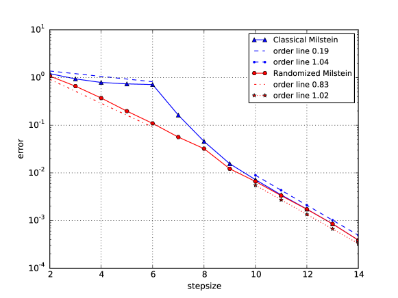
Figure 1. Numerical experiment for SDE (47): Step sizes versus $L^{2}$ errors

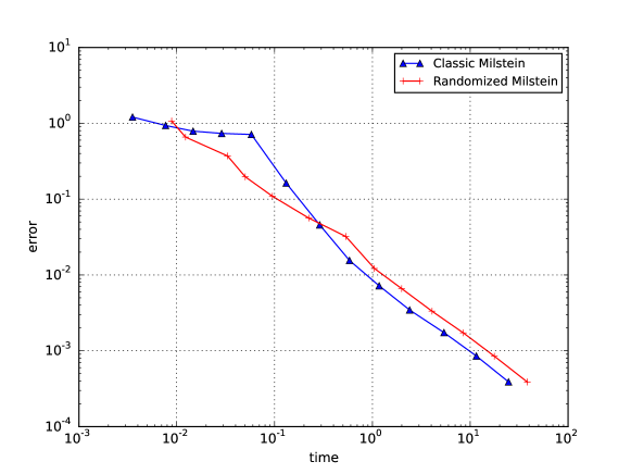
Figure 2. Numerical experiment for SDE (47): CPU time versus $L^{2}$ errors

References

• [1] W.-J. Beyn and R. Kruse. Two-sided error estimates for the stochastic theta method. Discrete Contin. Dyn. Syst. Ser. B, 14(2):389–407, 2010.
• [2] D. L. Burkholder. Martingale transforms. Ann. Math. Statist., 37:1494–1504, 1966.
• [3] J. M. C. Clark and R. J. Cameron. The maximum rate of convergence of discrete approximations for stochastic differential equations. In Stochastic differential systems (Proc. IFIP-WG 7/1 Working Conf., Vilnius, 1978), volume 25 of Lecture Notes in Control and Information Sci., pages 162–171. Springer, Berlin, 1980.
• [4] T. Daun. On the randomized solution of initial value problems. J. Complexity, 27(3-4):300–311, 2011.
• [5] E. Emmrich. Discrete versions of Gronwall’s lemma and their application to the numerical analysis of parabolic problems. TU Berlin, FB Mathematik, Preprint, 637-1999, 1999.
• [6] J. G. Gaines and T. J. Lyons. Random generation of stochastic area integrals. SIAM J. Appl. Math., 54(4):1132–1146, 1994.
• [7] M. B. Giles and L. Szpruch. Antithetic multilevel Monte Carlo estimation for multi-dimensional SDEs without Lévy area simulation. Ann. Appl. Probab., 24(4):1585–1620, 2014.
• [8] I. Gyöngy. A note on Euler’s approximations. Potential Anal., 8(3):205–216, 1998.
• [9] S. Haber. A modified Monte-Carlo quadrature. Math. Comp., 20:361–368, 1966.
• [10] S. Haber. A modified Monte-Carlo quadrature. II. Math. Comp., 21:388–397, 1967.
• [11] S. Heinrich and B. Milla. The randomized complexity of initial value problems. J. Complexity, 24(2):77–88, 2008.
• [12] M. Hutzenthaler, A. Jentzen, and P. E. Kloeden. Strong and weak divergence in finite time of Euler’s method for stochastic differential equations with non-globally Lipschitz continuous coefficients. Proc. R. Soc. Lond. Ser. A Math. Phys. Eng. Sci., 467(2130):1563–1576, 2011.
• [13] A. Jentzen and A. Neuenkirch. A random Euler scheme for Carathéodory differential equations. J. Comput. Appl. Math., 224(1):346–359, 2009.
• [14] B. Kacewicz. Optimal solution of ordinary differential equations. J. Complexity, 3(4):451–465, 1987.
• [15] B. Kacewicz. Almost optimal solution of initial-value problems by randomized and quantum algorithms. J. Complexity, 22(5):676–690, 2006.
• [16] P. E. Kloeden and A. Neuenkirch. The pathwise convergence of approximation schemes for stochastic differential equations. LMS J. Comput. Math., 10:235–253, 2007.
• [17] P. E. Kloeden and E. Platen. Numerical Solution of Stochastic Differential Equations. Springer, Berlin, third edition, 1999.
• [18] R. Kruse. Characterization of bistability for stochastic multistep methods. BIT, 52(1):109–140, 2012.
• [19] R. Kruse. Consistency and stability of a Milstein-Galerkin finite element scheme for semilinear SPDE. Stoch. Partial Differ. Equ. Anal. Comput., 2(4):471–516, 2014.
• [20] R. Kruse and Y. Wu. Error analysis of randomized Runge-Kutta methods for differential equations with time-irregular coefficients. Comput. Methods Appl. Math., 2017. (to appear).
• [21] X. Mao. Stochastic differential equations and applications. Horwood Publishing Limited, Chichester, second edition, 2008.
• [22] G. N. Milstein. Approximate integration of stochastic differential equations. Teor. Verojatnost. i Primenen., 19:583–588, 1974. in Russian.
• [23] G. N. Milstein. Approximate integration of stochastic differential equations. Theory Probab. Appl., 19(3):557–562, 1975. translated by K. Durr.
• [24] G. N. Milstein. Numerical integration of stochastic differential equations, volume 313 of Mathematics and its Applications. Kluwer Academic Publishers Group, Dordrecht, 1995. Translated and revised from the 1988 Russian original.
• [25] G. N. Milstein and M. V. Tretyakov. Stochastic Numerics for Mathematical Physics. Scientific Computation. Springer-Verlag, Berlin, 2004.
• [26] P. M. Morkisz and P. Przybyłowicz. Optimal pointwise approximation of SDE’s from inexact information. J. Comput. Appl. Math., 324:85–100, 2017.
• [27] P. Przybyłowicz. Minimal asymptotic error for one-point approximation of SDEs with time-irregular coefficients. J. Comput. Appl. Math., 282:98–110, 2015.
• [28] P. Przybyłowicz. Optimal global approximation of SDEs with time-irregular coefficients in asymptotic setting. Appl. Math. Comput., 270:441–457, 2015.
• [29] P. Przybyłowicz and P. Morkisz. Strong approximation of solutions of stochastic differential equations with time-irregular coefficients via randomized Euler algorithm. Appl. Numer. Math., 78:80–94, 2014.
• [30] T. Rydén and M. Wiktorsson. On the simulation of iterated Itô integrals. Stochastic Process. Appl., 91(1):151–168, 2001.
• [31] M. N. Spijker. Stability and convergence of finite-difference methods, volume 1968 of Doctoral dissertation, University of Leiden. Rijksuniversiteit te Leiden, Leiden, 1968.
• [32] M. N. Spijker. On the structure of error estimates for finite-difference methods. Numer. Math., 18:73–100, 1971/72.
• [33] G. Stengle. Numerical methods for systems with measurable coefficients. Appl. Math. Lett., 3(4):25–29, 1990.
• [34] G. Stengle. Error analysis of a randomized numerical method. Numer. Math., 70(1):119–128, 1995.
• [35] F. Stummel. Approximation methods in analysis. Matematisk Institut, Aarhus Universitet, Aarhus, 1973. Lectures delivered during the spring term, 1973, Lecture Notes Series, No. 35.
• [36] M. Wiktorsson. Joint characteristic function and simultaneous simulation of iterated Itô integrals for multiple independent Brownian motions. Ann. Appl. Probab., 11(2):470–487, 2001.