A maximum entropy approach to H-theory: Statistical mechanics of hierarchical systems

Abstract

A novel formalism, called H-theory, is applied to the problem of statistical equilibrium of a hierarchical complex system with multiple time and length scales. In this approach, the system is formally treated as being composed of a small subsystem—representing the region where the measurements are made—in contact with a set of ‘nested heat reservoirs’ corresponding to the hierarchical structure of the system. The probability distribution function (pdf) of the fluctuating temperatures at each reservoir, conditioned on the temperature of the reservoir above it, is determined from a maximum entropy principle subject to appropriate constraints that describe the thermal equilibrium properties of the system. The marginal temperature distribution of the innermost reservoir is obtained by integrating over the conditional distributions of all larger scales, and the resulting pdf is written in analytical form in terms of certain special transcendental functions, known as the Fox $H$-functions. The distribution of states of the small subsystem is then computed by averaging the quasi-equilibrium Boltzmann distribution over the temperature of the innermost reservoir. This distribution can also be written in terms of $H$-functions. The general family of distributions reported here recovers, as particular cases, the stationary distributions recently obtained by Macêdo et al. [Phys. Rev. E 95, 032315 (2017)] from a stochastic dynamical approach to the problem.

I INTRODUCTION

Complex systems with multiple time and length scales occur frequently in many areas of physics and interdisciplinary fields, such as turbulence frisch , random-matrix theory mehta , high-energy collision physics wilk ; cosmicrays , and econophysics finance , to mention only a few. One common feature among many such systems is the appearance of probability distributions that deviate considerably from what one would expect (say, Gaussian or exponential behavior) on the basis of standard equilibrium statistical mechanics arguments. A great deal of effort has therefore been devoted to constructing physical models that generate such heavy-tailed distributions. One approach that has attracted considerable attention is the so-called nonextensive statistical mechanics formalism tsallis whereby a power-law distribution, known as the Tsallis distribution, is obtained by maximizing a nonextensive entropy that generalizes the Boltzmann entropy formula. Heavy-tailed distributions can also be accounted for by a superposition of two statistics—a procedure known in mathematics as compounding compounding and in physics as superstatistics beck . In particular, the Tsallis distribution can be readily obtained from the superstatistics approach by an appropriate choice of the weighting distribution beck . Furthermore, this choice of weighting distribution can be justified from both a Bayesian analysis sattin ; RCF and a maximum entropy principle based on the Boltzmann-Shannon entropy VakarinPRE2006 ; beckpre2007 ; Crooks2007 ; BeckPRE08 ; Dixit , thus circumventing the need to introduce a non-extensive entropy to justify the emergence of heavy-tailed distributions.

Recently, we introduced a general formalism SV1 ; SV2 ; ourPRE2017 that extends the superstatistics approach to multiscale systems and gives rise to a large family of heavy-tailed distributions labeled by the number $N$ of different scales present in the system. (Usual superstatistics corresponds to $N=1$ Sobyanin2011 .) In this hierarchical formalism, to which we refer as H-theory, it is assumed that at large scales the statistics of the system is described by a known distribution that contains a parameter (say, the temperature $T_{0}$) that characterizes the global equilibrium of the system. At short scales, however, the system deviates considerably from the large-scale distribution, owing to the complex multiscale dynamics (intermittency effects) of the system. The scale dependence of the relevant distributions can be effectively described by assuming that the environment (background) surrounding the system under investigation changes slowly in time. The dynamics of the background is then formulated as a set of hierarchical stochastic differential equations whose form is derived from simple physical constraints, yielding only two ‘universality classes’ for the stationary distributions of the background variables at each level of the hierarchy: i) a gamma distribution and ii) an inverse-gamma distribution. For both classes, analytical expressions are obtained for the marginal distribution of the background variable at the lowest level of the hierarchy in terms of Meijer $G$-functions, from which the heavy-tailed distribution of the fluctuating signal is computed (and also written in terms of $G$-functions). Here two classes of signal distributions are found ourPRE2017 according to the behavior at the tails: i) power-law decay and ii) stretched-exponential tail. Applications of the H-theory to empirical data from several systems, such as turbulence SV1 ; SV2 , financial markets ourPRE2017 , and random fiber lasers NatComm2017 have yielded excellent results.

The dynamical formulation of the H-theory reviewed in the preceding paragraph represents a ‘microscopic’ (i.e., small-scale) approach to the problem, in that it tries to model the fluctuations in the environment under which the system evolves by a set of stochastic differential equations, which in principle provides a full description of the time-dependent stationary joint distribution function of the background variables. In this paper we take an alternative, thermodynamic-like approach in which the background distribution will be derived from a maximum entropy principle, thus bypassing the need to specify the underlying dynamics. We remark that this weakening of the basic dynamical hypothesis of H-theory leads to a considerable expansion of its domain of applicability, which may now include complex multiscale systems with non-Markovian stochastic dynamics.

The main purpose of the paper is to present a unified maximum-entropy principle suitable for hierarchical complex systems in statistical equilibrium. The main idea in our approach is to write the Boltzmann-Shannon entropy of the system in terms of the local equilibrium distribution of states and the distributions of the background variables (‘local temperatures’) across the hierarchy. In other words, the system is treated as being effectively composed of a small system in thermal equilibrium with a set of nested ‘heat reservoirs’, where the temperature of each reservoir is allowed to fluctuate owing to the interaction between adjacent reservoirs in the hierarchy. By maximizing the entropy with respect to the conditional temperature distributions at each level of the hierarchy, subject to certain physically motivated constraints, we obtain a general family of distributions that includes two particular classes, namely the generalized gamma and the generalized inverse-gamma distributions.

The marginal distribution of temperature of the innermost reservoir (i.e., at the lowest level of the hierarchy) is obtained by integrating over the conditional distributions of all larger scales. Remarkably, the resulting distribution can be written explicitly in terms of a known special function, namely the Fox $H$-function. Averaging the quasi-equilibrium Boltzmann distribution of the small system over the temperature of the innermost reservoir then yields the marginal distribution of states, which can also be written in terms of Fox $H$-functions. Here again the distributions of states can be classified into two classes according to the tail behavior, namely the power-law and stretched-exponential classes. For a particular choice of constraints our generalized distributions recover the distribution obtained in Ref. ourPRE2017 in terms of Meijer $G$-functions. The H-theory described here thus provides a rather general framework to describe the statistics of fluctuations in complex systems with multiple time and length scales.

II Multiscale Systems

We consider a multiscale complex system that is characterized by $N$ well-separated time scales, $\tau_{i}$, $i=1,...,N$, in addition to a large decorrelation time $\tau_{0}$ above which fluctuations in the system are essentially uncorrelated. Let us order these timescales from smallest to largest: $\tau_{N}\ll\tau_{N-1}\ll\cdots\ll\tau_{1}\ll\tau_{0}$. Thus, if one samples the system at time intervals larger than or comparable to $\tau_{0}$, one will find the usual canonical distribution of states: $p(\boldsymbol{q}|\beta_{0})={\exp(-\beta_{0}E(\boldsymbol{q}))}/{Z(\beta_{0})}$, where $\boldsymbol{q}$ denotes the state variables, $\beta_{0}=1/k_{B}T_{0}$, with $T_{0}$ representing the ‘global’ temperature of the system, $E(\boldsymbol{q})$ is the energy of the state labeled by $\boldsymbol{q}$, and $Z(\beta_{0})$ is the large-scale partition function defined by $Z(\beta_{0})=\int\exp(-\beta_{0}E(\boldsymbol{q}))d\boldsymbol{q}$.

At short time scales (say, smaller than the smallest characteristic time $\tau_{N}$), the distribution of states $p(\boldsymbol{q})$ deviates considerably from the large-scale distribution $p(\boldsymbol{q}|\beta_{0})$, owing to the complex multiscale dynamics of the system. In this scenario, it is convenient to consider the system as being composed of a small subsystem—corresponding to the effective region where the measurements are performed—and a large subsystem that has a slow internal dynamics characterized by several, hierarchically arranged timescales. Thus, in contrast to the usual canonical formulation, the large subsystem can no longer be treated as a single ‘heat reservoir’ with a fixed temperature. Instead, it must be viewed as a set of $N$ ‘nested reservoirs’ where each reservoir is described by a fluctuating temperature $T_{j}$, $j=1,...,N$. Physically, the fluctuations in these ‘local temperatures’ are caused by the interaction (exchange of energy) between adjacent subsystems in the hierarchy, in analogy with the phenomenon of intermittency in turbulence frisch .

Invoking Bayes’s theorem, the joint equilibrium distribution $p(\boldsymbol{q},\beta_{1},...,\beta_{N})$, where $\beta_{j}=1/k_{B}T_{j}$, can be factorized as

$$p(\boldsymbol{q},\boldsymbol{\beta})=p(\boldsymbol{q}|\boldsymbol{\beta})p(\boldsymbol{\beta}).$$ (1)

where we introduced the notation $\boldsymbol{\beta}\equiv(\beta_{1},\beta_{2},...,\beta_{N})$. Because of the hierarchical nature of our system, we assume that the conditional distribution $p(\boldsymbol{q}|\boldsymbol{\beta})$ depends only on the inverse temperature $\beta_{N}$ of the innermost reservoir, since this is the only reservoir in ‘direct contact’ with the small subsystem, and so we write

$$p(\boldsymbol{q}|\boldsymbol{\beta})=p(\boldsymbol{q}|\beta_{N}).$$ (2)

This means that the physical constraints imposed on the system at the large scale (and which fix the global temperature $T_{0}$) are not directly felt at the small scales but rather are transferred down the hierarchy through the intervening scales. Under these assumptions, the marginal distribution $p(\boldsymbol{q})$ can be written as

$$P(\boldsymbol{q})=\int_{0}^{\infty}P(\boldsymbol{q}|\beta_{N})p(\beta_{N})d\beta_{N},$$ (3)

where the probability distribution $p(\beta_{N})$ of the local inverse temperature $\beta_{N}$ is given by

$$p(\beta_{N}) =\int_{0}^{\infty}\cdots\int_{0}^{\infty}p(\boldsymbol{\beta})d\beta_{1}\cdots d\beta_{N-1}.$$ (4)

Owing to the separation of timescales, it is reasonable to assume that the small subsystem, which has a fast dynamics, is in local equilibrium with its immediate vicinity whose inverse temperature $\beta_{N}$ changes much more slowly. In other words, over short time periods (during which $\beta_{N}$ does not change appreciably) the conditional probability $p(\boldsymbol{q}|\beta_{N})$ can be described by a Boltzmann distribution:

$$p(\boldsymbol{q}|\beta_{N})=\frac{\exp(-\beta_{N}E(\boldsymbol{q}))}{Z(\beta_{N})}.$$ (5)

The remaining task then is to find the distribution $p(\beta_{N})$ of the local inverse temperature which encodes the complex dynamics of the multiscale background. This can be done by exploiting the hierarchical structure of the system, as argued below.

We assume that a subsystem (reservoir) at a given level $j$ of the hierarchy interacts only with the reservoir at the next level up the hierarchy, and so we write the joint distribution $p(\boldsymbol{\beta})$ as

$$p(\boldsymbol{\beta})=\prod_{j=1}^{N}f(\beta_{j}|\beta_{j-1}),$$ (6)

where $f(\beta_{j}|\beta_{j-1})$ denotes the probability density of $\beta_{j}$ conditioned on a fixed value of $\beta_{j-1}$. In view of (4) and (6), the marginal distribution $p(\beta_{N})$ can now be written as

$$p(\beta_{N}) =\int_{0}^{\infty}\cdots\int_{0}^{\infty}\prod_{j=1}^{N}f(\beta_{j}|\beta_{j-1})d\beta_{1}\cdots d\beta_{N-1},$$ (7)

In this way, our task has been reduced to computing the conditional distributions $f(\beta_{j}|\beta_{j-1})$, for $j=1,...,N$. In the next section we shall use a maximum entropy approach to solve this problem.

III Entropy Formulation

III.1 Multiscale entropy

As usual, we define the information entropy of the joint distribution $p(\boldsymbol{q},\boldsymbol{\beta})$ by

$$S[p(\boldsymbol{q},\boldsymbol{\beta})]=-\int\int p(\boldsymbol{q},\boldsymbol{\beta})\ln p(\boldsymbol{q},\boldsymbol{\beta}){d\boldsymbol{q}}d\boldsymbol{\beta},$$ (8)

where we use the shorthand notation $d\boldsymbol{\beta}=\prod_{j=1}^{N}d\beta_{j}$. In view of (1), (2) and (6), the entropy (8) can be rewritten as

$$S[p(\boldsymbol{q},\boldsymbol{\beta})] =\int p(\boldsymbol{\beta})s(\beta_{N}){d\boldsymbol{\beta}}-\sum_{k=1}^{N}\int p(\boldsymbol{\beta})\ln f(\beta_{k}|\beta_{k-1})d\boldsymbol{\beta}_{,}$$ (9)

where $s(\beta_{N})$ is the thermodynamic entropy of the small subsystem:

$$s(\beta_{N})=-\int p(\boldsymbol{q}|\beta_{N})\ln p(\boldsymbol{q}|\beta_{N})d\boldsymbol{q},$$ (10)

which is a multiscale generalization of the entropy described in superstatistics beckpre2007 ; Dixit for the case $N=1$. Let us also define the entropy at level $j$, for $j=0,...,N-1$, as the average of $s(\beta_{N})$ over all scales below this level, that is,

$$s(\beta_{j})=\int s(\beta_{N})p(\boldsymbol{\beta})d\beta_{j+1}\cdots d\beta_{N}.$$ (11)

We now seek to maximize (9) with respect to (w.r.t.) the distributions $f(\beta_{j}|\beta_{j-1})$. To this end, let us first discuss the constraints under which we shall carry out this maximization procedure.

III.2 Constraints

The first set of constraints is given by the usual normalization condition

$$\int f(\beta_{j}|\beta_{j-1})d\beta_{j}=1,\qquad j=1,...,N.$$ (12)

The second set of constraints entails the choice of a moment to be kept fixed in the maximization procedure. Usually, the first moment (mean) is the preferred choice VakarinPRE2006 ; Dixit . Here, however, we shall adopt a more general approach and fix the $r$-th moment of the distributions $f(\beta_{j}|\beta_{j-1})$. More specifically, we require that

$$\int\beta_{j}^{r}f(\beta_{j}|\beta_{j-1})d\beta_{j}=\beta_{j-1}^{r},\qquad j=1,...,N,$$ (13)

for some arbitrary real $r\neq 0$ (not necessarily an integer). Notice that (13) implies that

$$\langle\beta_{j}^{r}\rangle\equiv\int\beta_{j}^{r}p(\boldsymbol{\beta}_{j})d\boldsymbol{\beta}_{j}=\beta_{0}^{r},\qquad j=1,...,N,$$ (14)

where we introduced the notation

$$\boldsymbol{\beta}_{j}\equiv(\beta_{1},...,\beta_{j}).$$

Eq. (14) can be seen as a generalized equilibrium condition in the sense that the average value of $\beta_{j}^{r}$ is the same at all levels of the hierarchy.

As an additional constraint we use the average entropy

$$\langle s(\beta_{N})\rangle\equiv\int\ s(\beta_{N})p(\boldsymbol{\beta})d\boldsymbol{\beta}=s(\beta_{0}),$$ (15)

where $s(\beta_{0})$ is fixed. It then follows from definition (11) that the average entropy is the same across all scales:

$$\langle s(\beta_{j})\rangle\equiv\int\ s(\beta_{j})p(\boldsymbol{\beta}_{j})d\boldsymbol{\beta}_{j}=s(\beta_{0}),\qquad j=1,...,N,$$ (16)

which is a reasonable equilibrium condition. Furthermore, we shall assume that the thermodynamic entropy defined in (10) satisfies the following relation

$$s(\beta_{N})\sim s_{0}\ln\beta_{N},$$ (17)

where $s_{0}$ is a constant and the notation $\sim$ indicates equality except for an additive constant. (In other words, $f(x)\sim g(x)$ means here that $f(x)=g(x)+C$, where $C$ is a constant.) We recall that relation (17) is valid for a large class of systems, such as those that obey the equipartition theorem, for which the internal energy is proportional to the temperature VakarinPRE2006 ; Dixit .

We also make the assumption that the distribution $f_{k}(\beta_{k}|\beta_{k-1})$ is invariant under a rescaling of the variables $\beta\rightarrow\lambda\beta$:

$$\begin{split}f_{k}(\beta_{k}|\beta_{k-1})d\beta_{k}=f_{k}(\lambda\beta_{k}|\lambda\beta_{k-1})d(\lambda\beta_{k}).\end{split}$$ (18)

Physically, this means that the temperature distributions should remain of the same form regardless of the temperature scale one chooses. Now, if we make $\lambda=1/\beta_{k-1}$ in (18) we get

$$\begin{split}f_{k}(\beta_{k}|\beta_{k-1})d\beta_{k}=g_{k}\left(\frac{\beta_{k}}{\beta_{k-1}}\right)\frac{d\beta_{k}}{\beta_{k-1}}=g_{k}(u)du,\end{split}$$ (19)

for some function $g_{k}(u)$, where $u=\beta_{k}/\beta_{k-1}$. Relation (19) leads to the following two useful relations that are proven in Appendix A:

$$\int p(\boldsymbol{\beta}_{k})\ln\beta_{k}d{\boldsymbol{\beta}_{k}}\;\sim\int p(\boldsymbol{\beta}_{j})\ln\beta_{j}d\boldsymbol{\beta}_{j},\qquad\mbox{for $j\leq k$},$$ (20)

and

$$\int p(\boldsymbol{\beta}_{k})\ln f(\beta_{k}|\beta_{k-1})d{\boldsymbol{\beta}_{k}}\;\sim-\int p(\boldsymbol{\beta}_{j})\ln\beta_{j}d\boldsymbol{\beta}_{j},\qquad\mbox{for $j<k$}.$$ (21)

Now, inserting (17) into (11) and using (20), one finds that

$$s(\beta_{j})=s_{0}\ln\beta_{j}+s_{j},$$ (22)

where $s_{j}$ is a constant that does not depend on $\beta_{j}$. In view of this relation, the constraint (16) can be written as

$$\int\left(\ln\beta_{j}\right)p(\boldsymbol{\beta}_{j})d\boldsymbol{\beta}_{j}=c_{j},$$ (23)

where $c_{j}$ is a constant.

III.3 Entropy maximization

In order to maximize (9) w.r.t. $f(\beta_{j}|\beta_{j-1})$, for any given $j$, it is necessary to make it explicit the dependence of $S[p(\boldsymbol{q},\boldsymbol{\beta})]$ on $f(\beta_{j}|\beta_{j-1})$. To this end, we first note that on use of (6) and (12) we can rewrite (9) as

$$S[p(\boldsymbol{q},\boldsymbol{\beta})] =\int s(\beta_{j})p(\boldsymbol{\beta}_{j}){d\boldsymbol{\beta}_{j}}-\sum_{k=1}^{j-1}\int p(\boldsymbol{\beta}_{k})\ln f(\beta_{k}|\beta_{k-1})d{\boldsymbol{\beta}_{k}}$$ (24)

$$-\int p(\boldsymbol{\beta}_{j})\ln f(\beta_{j}|\beta_{j-1})d{\boldsymbol{\beta}_{j}}-\sum_{k=j+1}^{N}\int p(\boldsymbol{\beta}_{k})\ln f(\beta_{k}|\beta_{k-1})d{\boldsymbol{\beta}_{k}}.$$ (25)

Now using (21) and (22) in (24), one finds that

$$S[p(\boldsymbol{q},\boldsymbol{\beta})] \sim c_{j}\int p(\boldsymbol{\beta}_{j})\ln\beta_{j}{d\boldsymbol{\beta}_{j}}-\int p(\boldsymbol{\beta}_{j})\ln f(\beta_{j}|\beta_{j-1})d\boldsymbol{\beta}_{j}-\sum_{k=1}^{j-1}\int p(\boldsymbol{\beta}_{k})\ln f(\beta_{k}|\beta_{k-1})d\boldsymbol{\beta}_{k},$$ (26)

where $c_{j}=N-j-s_{0}$. Note that the entropy $S[p(\boldsymbol{q},\boldsymbol{\beta})]$ depends on $f(\beta_{j}|\beta_{j-1})$ only through the first two terms in the right hand side of (26).

Maximizing (26) w.r.t. $f(\beta_{j}|\beta_{j-1})$, subject to the constraints (12), (13) and (23), yields

$$\int\left[\ln f(\beta_{j}|\beta_{j-1})+A_{j}+B_{j}\beta_{j}^{r}+C_{j}\ln\beta_{j}\right]\delta_{j}p(\boldsymbol{\beta}_{j})d\boldsymbol{\beta}_{j}=0,$$ (27)

where $A_{j}$, $B_{j}$, and $C_{j}$ are Lagrange multipliers and $\delta_{j}p(\boldsymbol{\beta}_{j})\equiv p(\boldsymbol{\beta}_{j-1})\delta f(\beta_{j}|\beta_{j-1})$. The solution to (27) takes the form

$$f(\beta_{j}|\beta_{j-1})=e^{-A_{j}}\beta_{j}^{-C_{j}}\exp{\left(-B_{j}\beta_{j}^{r}\right)}.$$ (28)

To enforce the constraint (13) we choose $B_{j}=\alpha_{j}/\beta_{j-1}^{r}$ and set $C_{j}=-r\alpha_{j}+1$, where $\alpha_{j}>0$. Using these parameters in (28) one obtains the following general distribution:

$$f_{j}(\beta_{j}|\beta_{j-1})=\frac{|r|\alpha_{j}^{\alpha_{j}}}{\beta_{j}\Gamma(\alpha_{j})}\left(\frac{\beta_{j}}{\beta_{j-1}}\right)^{r\alpha_{j}}\exp\left[{-\alpha_{j}\left(\frac{\beta_{j}}{\beta_{j-1}}\right)^{r}}\right].$$ (29)

For $r>0$ this distribution corresponds to the generalized gamma distribution, whereas for $r<0$ it gives the generalized inverse gamma distribution.

We note furthermore that for the particular case $r=1$ the distribution (29) yields the usual gamma distribution,

$$f_{j}(\beta_{j}|\beta_{j-1})=\frac{\left(\alpha_{j}/\beta_{j-1}\right)^{\alpha_{j}}}{\Gamma(\alpha_{j})}{\beta_{j}}{}^{\alpha_{j}-1}\exp\left({-\frac{\alpha_{j}\beta_{j}}{\beta_{j-1}}}\right),$$ (30)

whereas for $r=-1$ it gives the standard inverse gamma distribution:

$$f_{j}(\beta_{j}|\beta_{j-1})=\frac{\left(\alpha_{j}\beta_{j-1}\right)^{\alpha_{j}}}{\Gamma(\alpha_{j})}{\beta_{j}}^{-\alpha_{j}-1}\exp\left({-\frac{\alpha_{j}\beta_{j-1}}{\beta_{j}}}\right).$$ (31)

It is interesting to note that the generalized inverse gamma distribution has recently been used to model wealth distribution in ancient Egypt egypt . The Weibull and the Frechet distributions, which are particular cases of the generalized gamma and generalized inverse-gamma distributions, respectively, have also found important applications in extreme value statistics extreme_val and sum of correlated random variables Weibull . Here, however, our interest is to use (29) not so much as a standalone distribution but rather as a means to obtain the distribution $p(\beta_{N})$ of inverse temperatures at the innermost reservoir, from which the distribution of states $p(\boldsymbol{q}$) can be found. This is done next.

IV The equilibrium distributions

As discussed in Sec. II, the complex dynamics of the large system (background) is felt by the small subsystem only through the fluctuations of the inverse temperature $\beta_{N}$ of the innermost reservoir. Thus, in order to determine the marginal distribution of states $p(\boldsymbol{q})$ of the small subsystem, it is necessary first to compute the distribution $p(\beta_{N})$; see (3). It is remarkable that both these distributions can be obtained in analytical form in terms of some special transcendental functions known as the Fox $H$-functions Hfunction , as shown below.

IV.1 The background distribution

The marginal distribution $p(\beta_{N})$ at the lowest level of the hierarchy is given by (7), where each of the distributions $f(\beta_{j}|\beta_{j-1})$ appearing in this expression is as shown in (29). In computing the multiple integrals in (7) the cases $r>0$ and $r<0$ need to be treated separately, but for both cases these integrals can be calculated explicitly in terms of the Fox $H$-functions.

As shown in Appendix B, for the case $r>0$ one finds

$$p(\beta_{N})=\omega_{\rho}\Omega H_{0,N}^{N,0}\left(\begin{array}[]{c}{-}\\ {(\boldsymbol{\alpha}-\rho{\bf 1},\rho{\bf 1})}\end{array}\bigg{|}\frac{\omega_{\rho}\beta_{N}}{\beta_{0}}\right),$$ (32)

whilst for $r<0$ the result is

$$p(\beta_{N})=\frac{\Omega}{\omega_{\rho}}H_{N,0}^{0,N}\left(\begin{array}[]{c}{((1-\rho){\bf 1}-\boldsymbol{\alpha},\rho{\bf 1})}\\ {-}\end{array}\bigg{|}\frac{\beta_{N}}{\omega_{\rho}\beta_{0}}\right),$$ (33)

where $\rho=1/|r|$, $\omega_{\rho}=\prod_{j=1}^{N}\alpha_{j}^{\rho}$, and $\Omega=1/\left(\beta_{0}\Gamma(\boldsymbol{\alpha})\right)$. Here we have introduced the vector notation ${\boldsymbol{\alpha}}\equiv(\alpha_{1},\dots,\alpha_{N})$ and $\Gamma({\bf a})\equiv\prod_{j=1}^{N}\Gamma(a_{j})$. We have also used a dash in the top row of the $H$-function in (32) and in the low row of the $H$-function in (33) to indicate that the respective parameters are not present.

We note in passing that after setting $|r|=1$ in expressions (32) and (33) we recover the two classes of universality for the background distributions obtained in Ref. ourPRE2017 from a stochastic dynamical model. To see this, we note that for $\rho=1$ the set of parameters $\rho{\bf 1}\equiv(\rho,...,\rho)$ appearing in each of the $H$-functions above becomes simply the identity vector, in which case the $H$-function reduces to a simpler function, namely the Meijer $G$-function Hfunction . Setting $\rho=1$ in (32) then yields

$$p(\beta_{N})=\omega\Omega G_{0,N}^{N,0}\left(\begin{array}[]{c}{-}\\ {\boldsymbol{\alpha}-{\bf 1}}\end{array}\bigg{|}\frac{\omega\beta_{N}}{\beta_{0}}\right),$$ (34)

whilst from (33) one has

$$p(\beta_{N})=\frac{\Omega}{\omega}G_{N,0}^{0,N}\left(\begin{array}[]{c}{-\boldsymbol{\alpha}}\\ {-}\end{array}\bigg{|}\frac{\beta_{N}}{\beta_{0}\omega}\right),$$ (35)

where $\omega=\prod_{j=1}^{N}\alpha_{j}$. In comparing the distributions (34) and (35) with the corresponding expressions given Ref. ourPRE2017 one has to bear in mind that there the distributions are written in terms of a variable $\varepsilon_{N}$ which corresponds in the notation of the present paper to $1/\beta_{N}$.

IV.2 The distribution of states

In view of (3) and (5), the marginal distribution of states $p(\boldsymbol{q})$ of the small subsystem can be written as

$$p(\boldsymbol{q}) =\int_{0}^{\infty}\frac{\exp(-\beta_{N}E(\boldsymbol{q}))}{Z(\beta_{N})}p(\beta_{N})d\beta_{N}$$ (36)

where $p(\beta_{N})$ is given by either (32) or (33). In order to carry out this integral one needs to know the dependence of the partition function $Z(\beta_{N})$ on $\beta_{N}$. In view of the fact that $S(\beta)\sim\ln Z(\beta)$, it then follows from assumption (17) that $Z(\beta_{N})\sim\beta_{N}^{-\gamma}$, for some exponent $\gamma>0$, and so we write

$$Z(\beta_{N})=Z(\beta_{0})\left(\frac{\beta_{N}}{\beta_{0}}\right)^{-\gamma}.$$ (37)

Inserting (37) into (36) yields

$$p(\boldsymbol{q}) =\frac{1}{Z(\beta_{0})}\int_{0}^{\infty}\left(\frac{\beta_{N}}{\beta_{0}}\right)^{\gamma}\exp\left(-\beta_{N}E(\boldsymbol{q})\right)p(\beta_{N})d\beta_{N}$$ (38)

It is also remarkable that this integral can be carried out explicitly in terms of Fox $H$-functions for both classes of background distributions, with the resulting distributions being classified into two classes according to the behavior at the tails, as follows:

i) Power-law class. This is the case when $r>0$. Upon inserting (32) into (38) and using a convolution property of the $H$-function Hfunction , the resulting integral can be performed explicitly (see Appendix C), yielding

$$p(E)=\frac{1}{Z(\beta_{0})\omega_{\rho}^{\gamma}\Gamma(\boldsymbol{\alpha})}H_{N,1}^{1,N}\left(\begin{array}[]{c}{((1-\gamma\rho){\bf 1}-\boldsymbol{\alpha},\rho{\bf 1})}\\ {(0,1)}\end{array}\bigg{|}\frac{\beta_{0}E}{\omega_{\rho}}\right).$$ (41)

Here we have omitted the state variable $\boldsymbol{q}$ for simplicity of notation, with the understanding that $p(E)$ denotes the probability of a state $\boldsymbol{q}$ with energy $E(\boldsymbol{q})$. From the asymptotic expansion of the $H$-function for large arguments one finds (Hfunction, ) that the $p(E)$ decays as a power-law for large values of $E$:

$$p(E)\sim\sum_{j=1}^{N}\frac{c_{j}}{E^{\gamma+|r|\alpha_{j}}},\quad\mbox{for}\quad E\to\infty,$$ (42)

where the $c_{i}$’s are constants. To illustrate the power-law class of distributions we show in Fig. 1 some plots of the function $p(E)$ given in (41) for cases where $\gamma=1$, $\beta_{0}=1$, $Z(\beta_{0})=1$, and $\alpha_{j}=\alpha=1.0$. The values of the parameters $N$ and $r$ for each plot is indicated in the caption of the figure. The main plots in Fig. 1 are in semilogarithmic scale, whilst the insets show the same data in log-log scale. One clearly sees from Figs. 1(a) and 1(b) that the smaller the value of the parameter $r$, for $N$ fixed, the heavier the tail of the distribution. This is in agreement with the aympotic behavior given in (42) which shows that the exponent of the power law decreases as $r$ decreases. Similarly, from Figs. 1(c) and 1(d) one sees that the larger the number $N$ of scales, for $r$ fixed, the heavier the tails. Note, however, that the exponent of the power-law does not depend on $N$; see (42). It is instead the prefactor that increases with $N$, since we are taking $\alpha_{j}=\alpha$, for $j=1,...,N$, thus causing a slower decay of the tail.

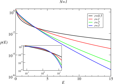
(a)

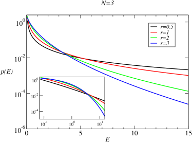
(b)

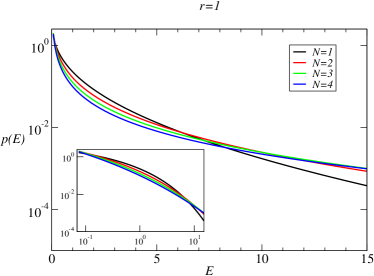
(c)

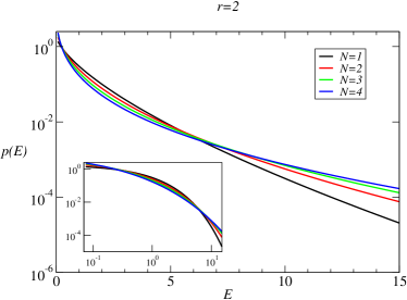
(d)

Figure 1: (Color online) (a) Distribution of states $p(E)$ for the power-law class for the following values of parameters: (a) $N=1$, $r=0.5,1,2,3$; (b) $N=3$, $r=0.5,1,2,3$; (c) $r=1$, $N=1,2,3,4$; and (d) $r=2$, $N=1,2,3,4$. In all cases shown here we have used $\gamma=1$, $\beta_{0}=1$, $Z(\beta_{0})=1$, and $\alpha_{j}=\alpha=1.0$, for $j=1,...,N$.

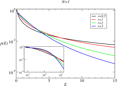
(a)

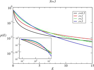
(b)

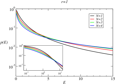
(c)

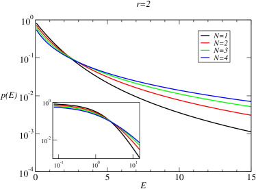
(d)

Figure 2: (Color online) Distribution of states $p(E)$ for the stretched exponential class with the same choice of parameters as in Fig. 1.

ii) Stretched-exponential class. This corresponds to the case $r<0$. Here the integral (38), with $p(\beta_{N})$ as given in (33), can be written as

$$p(E)=\frac{\omega_{\rho}^{\gamma}}{Z(\beta_{0})\Gamma(\boldsymbol{\alpha})}H_{0,N+1}^{N+1,0}\left(\begin{array}[]{c}{-}\\ {(\boldsymbol{\alpha}-\gamma\rho{\bf 1},\rho{\bf 1}),(0,1)}\end{array}\bigg{|}\omega_{\rho}\beta_{0}E\right),$$ (45)

as also shown in Appendix C. The asymptotic behavior in this case is given by a modified stretched exponential:

$$\ p(E)\sim{E^{\theta}}{\exp\left[-A(\omega_{\rho}\beta_{0}E)^{1/(\rho N+1)}\right]},\quad\mbox{for}\quad E\to\infty,$$ (46)

where $\theta=N(\bar{\alpha}-\gamma\rho-1/2)/(\rho N+1)$, $\bar{\alpha}=(1/N)\sum_{i=1}^{N}\alpha_{i}$ and $A=(\rho N+1)\rho^{-\rho N/(\rho N+1)}$. Some illustrative plots of the function $p(E)$ given in (45) are shown in Fig. 2 for the same choice of parameters as in Fig. 1. The same qualitative dependence of the tails on the parameters $N$ and $r$ are observed here: the larger the value of $N$ or the smaller the choice of $r$, the heavier the tails. This behavior is in agreement with (46) which shows that the exponent of the stretched exponential decreases with both the increase of $N$ and the decrease of $r$.

We note in passing that the particular cases $r=\pm 1$ yield results consistent with those obtained in Ref. ourPRE2017 , in that the corresponding distributions can also be written in terms of $G$-functions. For $\rho=1$ the expression (41) simplifies to

$$p(E)=\frac{1}{Z(\beta_{0})\omega^{\gamma}\Gamma(\boldsymbol{\alpha})}G_{N,1}^{1,N}\left(\begin{array}[]{c}{(1-\gamma){\bf 1}-\boldsymbol{\alpha}}\\ 0\end{array}\bigg{|}\frac{\beta_{0}E}{\omega}\right),$$ (47)

whereas the distribution (45) reads

$$p(E)=\frac{\omega^{\gamma}}{Z(\beta_{0})\Gamma(\boldsymbol{\alpha})}G_{0,N+1}^{N+1,0}\left(\begin{array}[]{c}-\\ {\boldsymbol{\alpha}-\gamma{\bf 1},0}\end{array}\bigg{|}\omega\beta_{0}E\right).$$ (48)

V Conclusions

In this paper, we have used a maximum entropy principle to derive a generalized version of the multicanonical formalism (H-theory) introduced in Refs. SV2 ; ourPRE2017 . In our approach the system is considered to be effectively composed of a small subsystem in thermal equilibrium with a hierarchical set of heat reservoirs, whose local temperatures fluctuate owing to weak interactions between adjacent reservoirs. We characterized the joint equilibrium distribution of the state variables and the local inverse temperatures by means of its Shannon information entropy. This entropy was maximized with respect to the conditional temperature distributions at each level of the hierarchy, subject to certain physically motivated constraints. The large family of distributions that were found by this procedure can be grouped into two classes: the generalized gamma and the generalized inverse-gamma distributions. The knowledge of these conditional distributions of inverse temperatures allowed us to obtain the marginal distribution $p(\beta_{N})$ of the inverse temperature at the lowest level of the hierarchy, which was explicitly written for both classes in terms of the Fox $H$-functions.

The marginal distribution of states $p(\boldsymbol{q})$ was then obtained by averaging the conditional distribution of states $p(\boldsymbol{q}|\beta_{N})$ over the local inverse-temperature $\beta_{N}$ and the resulting distribution was also written in terms of Fox $H$-functions. These distributions exhibit heavy tails that can be classified into two classes, namely the power-law and stretched-exponential classes. The distributions derived in Ref. ourPRE2017 from a stochastic dynamical approach, which were written in terms of Meijer $G$-functions, were shown to be particular cases of the Fox $H$-functions obtained from the maximum entropy approach. The H-theory presented here thus provides a rather general framework to describe the statistics of fluctuations in complex systems with multiple time/space scales, quite irrespective of the detailed underlying dynamics. Applications of H-theory in the context of Eulerian and Lagrangian turbulence, mathematical finance and random lasers have had great success. Further applications of the generalized formalism presented here to other complex systems with multiple spatio-temporal scales are under current investigation.

Appendix A Derivation of (20) and (21)

First consider a term of the form

$$\int p(\boldsymbol{\beta}_{k})\ln\beta_{k}\;d\boldsymbol{\beta}_{k}.$$ (49)

This can be rewritten as

$$\int p(\boldsymbol{\beta}_{k})\ln\beta_{k}\;d\boldsymbol{\beta}_{k} =\int p(\boldsymbol{\beta}_{k})\left[\ln\left(\frac{\beta_{k}}{\beta_{k-1}}\right)+\ln\beta_{k-1}\right]d\boldsymbol{\beta}_{k}.$$ (50)

Upon using property (19) we then obtain

$$\int p(\boldsymbol{\beta}_{k})\ln\beta_{k}d\boldsymbol{\beta}_{k} =\left(\int g_{k}(u)\ln u\,du\right)\int p(\boldsymbol{\beta}_{k-1})d\boldsymbol{\beta}_{k-1}+\int p(\boldsymbol{\beta}_{k-1})\ln\beta_{k-1}\;d\boldsymbol{\beta}_{k-1}$$ (51)

$$=A_{k}+\int p(\boldsymbol{\beta}_{k-1})\ln\beta_{k-1}\;d\boldsymbol{\beta}_{k-1}$$ (52)

where $A_{k}=\int_{0}^{\infty}g_{k}(u)\ln u\,du$ is a constant. This implies that

$$\int p(\boldsymbol{\beta}_{k})\ln\beta_{k}d{\boldsymbol{\beta}_{k}}\;\sim\int p(\boldsymbol{\beta}_{k-1})\ln\beta_{k-1}d\boldsymbol{\beta}_{k-1},$$ (53)

where we recall that the notation $\sim$ implies equality, except for an irrelevant additive constant. If we repeat this procedure recursively we get (20).

Next consider terms of the form

$$\int p(\boldsymbol{\beta}_{k})\ln f(\beta_{k}|\beta_{k-1})d\boldsymbol{\beta}_{k}.$$ (54)

Using (19), we have

$$\int p(\boldsymbol{\beta}_{k})\ln f(\beta_{k}|\beta_{k-1})d{\boldsymbol{\beta}_{k}} =\int p(\boldsymbol{\beta}_{k})\ln\left[\frac{1}{\beta_{k-1}}g_{k}\left(\frac{\beta_{k}}{\beta_{k-1}}\right)\right]d\boldsymbol{\beta}_{k}$$ (55)

$$=\int g(u)\ln g_{k}(u)du-\int p(\boldsymbol{\beta}_{k-1})\ln\beta_{k-1}d\boldsymbol{\beta}_{k-1}$$ (56)

$$=B_{k}-\int p(\boldsymbol{\beta}_{k-1})\ln\beta_{k-1}d\boldsymbol{\beta}_{k-1},$$ (57)

where $B_{k}=\int_{0}^{\infty}g_{k}(u)\ln g_{k}(u)\,du$. Neglecting this additive constant we can then write

$$\int p(\boldsymbol{\beta}_{k})\ln f(\beta_{k}|\beta_{k-1})d{\boldsymbol{\beta}_{k}}\;\sim-\int p(\boldsymbol{\beta}_{k-1})\ln\beta_{k-1}d\boldsymbol{\beta}_{k-1},$$ (58)

which in view of (20) yields (21), as desired.

Appendix B Derivation of (32) and (33)

Here we calculate $p(\beta_{N})$ explicitly in terms of Fox $H$-functions. We begin by introducing the variable

$$y=\frac{\beta_{N}}{\beta_{0}}=\prod_{j=1}^{N}\xi_{j},$$ (59)

where $\xi_{j}=\beta_{j}/\beta_{j-1}$, so that $p(\beta_{N})=g(y)/\beta_{0}$ and

$$g(y)=\int_{0}^{\infty}\cdots\int_{0}^{\infty}\prod_{j=1}^{N}g_{j}(\xi_{j})d\xi_{j}\delta(y-\xi_{1}\xi_{2}\cdots\xi_{N}).$$ (60)

For $r>0$ we obtain from (29) that

$$g_{j}(\xi_{j})=\frac{r\alpha_{j}^{\alpha_{j}}}{\Gamma(\alpha_{j})}\xi_{j}^{r\alpha_{j}-1}e^{-\alpha_{j}\xi_{j}^{r}},$$ (61)

whilst for $r<0$ we find

$$g_{j}(\xi_{j})=\frac{r^{\prime}\alpha_{j}^{\alpha_{j}}}{\Gamma(\alpha_{j})}\xi_{j}^{-r^{\prime}\alpha_{j}-1}e^{-\alpha_{j}\xi_{j}^{-r^{\prime}}},$$ (62)

where we defined $r^{\prime}=-r>0$.

Now applying the Mellin transform, defined as

$${\cal M}[g;s]\equiv\int_{0}^{\infty}dyy^{s-1}g(y),$$ (63)

to both sides of (60), we find

$${\cal M}[g;s]=\prod_{j=1}^{N}{\cal M}[g_{j};s],$$ (64)

where

$${\cal M}[g_{j};s]=\frac{\Gamma(\alpha_{j}+(s-1)/r)}{\alpha_{j}^{(s-1)/r}\Gamma(\alpha_{j})}$$ (65)

is the Mellin transform of (61) and

$${\cal M}[g_{j};s]=\alpha_{j}^{(s-1)/r^{\prime}}\frac{\Gamma(\alpha_{j}+(1-s)/r^{\prime})}{\Gamma(\alpha_{j})}$$ (66)

is the Mellin transform of (62). Next, we use the following property of the Fox $H$-function (Hfunction, ). If the Mellin transform of $g(y)$ is

$${\cal M}[g;s]=\frac{\lambda^{-s}\prod_{j=1}^{m}\Gamma(b_{j}+B_{j}s)\prod_{j=1}^{n}\Gamma(1-a_{j}-A_{j}s)}{\prod_{j=m+1}^{q}\Gamma(1-b_{j}-B_{j}s)\prod_{j=n+1}^{p}\Gamma(a_{j}+A_{j}s)}$$

then

$$g(y)=H_{p,q}^{m,n}\left(\begin{array}[]{l}(\boldsymbol{a},\boldsymbol{A})\\ (\boldsymbol{b},\boldsymbol{B})\end{array}\bigg{|}\lambda y\right),$$ (67)

where we introduced the notation $(\boldsymbol{x},\boldsymbol{X})\equiv\{(x_{1},X_{1}),\ldots,(x_{d},X_{d})\}$, with $d\in\{p,q\}$. Using (64), (65) and (67) we obtain (32), while using (64), (66) and (67) we get (33), as desired.

Appendix C Derivation of (41) and (45)

We start by considering the Laplace transform of the Fox $H$-function (Hfunction, )

$$\int_{0}^{\infty}dx\;x^{\gamma}e^{-sx}H_{p,q}^{m,n}\left(\begin{array}[]{l}(\boldsymbol{a},\boldsymbol{A})\\ (\boldsymbol{b},\boldsymbol{B})\end{array}\bigg{|}\lambda x\right)=s^{-(\gamma+1)}H_{p+1,q}^{m,n+1}\left(\begin{array}[]{l}(\boldsymbol{a},\boldsymbol{A}),(-\gamma,1)\\ (\boldsymbol{b},\boldsymbol{B})\end{array}\bigg{|}\lambda s^{-1}\right),$$ (68)

where $(\boldsymbol{x},\boldsymbol{X})\equiv\{(x_{1},X_{1}),\ldots,(x_{d},X_{d})\}$, with $d\in\{p,q\}$. Using the identities

$$H_{p,q}^{m,n}\left(\begin{array}[]{l}(\boldsymbol{a},\boldsymbol{A})\\ (\boldsymbol{b},\boldsymbol{B})\end{array}\bigg{|}z\right)=H_{q,p}^{n,m}\left(\begin{array}[]{l}({\bf 1}-\boldsymbol{b},\boldsymbol{B})\\ ({\bf 1}-\boldsymbol{a},\boldsymbol{A})\end{array}\bigg{|}\frac{1}{z}\right)$$ (69)

and

$$z^{\sigma}H_{p,q}^{m,n}\left(\begin{array}[]{l}(\boldsymbol{a},\boldsymbol{A})\\ (\boldsymbol{b},\boldsymbol{B})\end{array}\bigg{|}z\right)=H_{p,q}^{m,n}\left(\begin{array}[]{l}(\boldsymbol{a}+\sigma\boldsymbol{A},\boldsymbol{A})\\ (\boldsymbol{b}+\sigma\boldsymbol{B},\boldsymbol{B})\end{array}\bigg{|}z\right)$$ (70)

we may rewrite (68) as

$$\int_{0}^{\infty}dxx^{\gamma}e^{-sx}H_{p,q}^{m,n}\left(\begin{array}[]{l}(\boldsymbol{a},\boldsymbol{A})\\ (\boldsymbol{b},\boldsymbol{B})\end{array}\bigg{|}\lambda x\right)=\frac{1}{\lambda^{\gamma+1}}H_{q,p+1}^{n+1,m}\left(\begin{array}[]{l}({\bf 1}-\boldsymbol{b}-(\gamma+1)\boldsymbol{B},\boldsymbol{B})\\ ({\bf 1}-\boldsymbol{a}-(\gamma+1)\boldsymbol{A},\boldsymbol{A}),(0,1)\end{array}\bigg{|}\frac{s}{\lambda}\right).$$ (71)

We are now in position to calculate the Laplace transform of $p(\beta_{N})$. Using (32) and (71), we get for the case $r>0$:

$$\int_{0}^{\infty}d\beta_{N}\;\beta_{N}^{\gamma}e^{-\beta_{N}E}p(\beta_{N})=\frac{\beta_{0}^{\gamma}}{\omega_{\rho}^{\gamma}\Gamma(\boldsymbol{\alpha})}H_{N,1}^{1,N}\left(\begin{array}[]{c}{((1-\gamma\rho){\bf 1}-\boldsymbol{\alpha},\rho{\bf 1})}\\ {(0,1)}\end{array}\bigg{|}\frac{\beta_{0}E(\boldsymbol{q})}{\omega_{\rho}}\right).$$ (72)

Similarly, in view of (33), the result for $r<0$ is

$$\int_{0}^{\infty}d\beta_{N}\;\beta_{N}^{\gamma}e^{-\beta_{N}E}p(\beta_{N})=\frac{(\beta_{0}\omega_{\rho})^{\gamma}}{\Gamma(\boldsymbol{\alpha})}H_{0,N+1}^{N+1,0}\left(\begin{array}[]{c}{-}\\ {(\boldsymbol{\alpha}-\gamma\rho{\bf 1},\rho{\bf 1}),(0,1)}\end{array}\bigg{|}\omega_{\rho}\beta_{0}E(\boldsymbol{q})\right).$$ (73)

Using (72) and (73) we obtain (41) and (45) respectively.

References

- (1) U. Frisch, Turbulence: the Legacy of A. N. Kolmogorov (Cambridge University Press, Cambridge, 1995).
- (2) M. L. Mehta, Random Matrices (Elsevier, Amsterdam, 2004).
- (3) G. Wilk and Z. Wlodarczyk, Eur. Phys. J. A 48, 161 (2012).
- (4) C. Beck, Eur. Phys. J. A 40, 267 (2009); and references therein.
- (5) S. Ghashghaie, W. Breymann, J. Peinke, P. Talkner and Y. Dodge, Nature 381, 767–770 (1996).
- (6) C. Tsallis, J. Stat. Phys. 52, 479 (1988); Introduction to Nonextensive Statistical Mechanics (Springer, New York, 2009).
- (7) O. Barndor-Nielsen, J. Kent, and M. Srensen, Int. Stat. Rev. 50, 145 (1982); S. D. Dubey, Metrika 16, 27 (1970).
- (8) C. Beck, Phys. Rev. Lett. 87, 180601 (2001); Europhys. Lett. 64, 151 (2003); Phys. Rev. Lett. 98, 064502 (2007).
- (9) F. Sattin, Eur. Phys. J. B 49, 219 (2006) .
- (10) G. L. Vasconcelos and D. S. P. Salazar, Rev. Cub. de Fís. 29, 1E (2012).
- (11) S. Abe, C. Beck and E. Cohen, Phys. Rev. E. 76, 031102 (2007).
- (12) G. E. Crooks, Phys. Rev. E 75, 041119 (2007).
- (13) E. Vakarin and J. Badiali, Phys. Rev. E. 74, 036120 (2006).
- (14) E. der Straeten and C. Beck, Phys. Rev. E. 78, 051101 (2008).
- (15) P. Dixit, Phys. Chem. Chem. Phys 17, 13000-13005 (2015).
- (16) D. S. P. Salazar and G. L. Vasconcelos, Phys. Rev. E 82, 047301 (2010).
- (17) D. S. P. Salazar, G. L. Vasconcelos, Phys. Rev. E . 86, 050103(R) (2012).
- (18) A. M. S. Macêdo, I. R. R. González, D. S. P. Salazar and G. L. Vasconcelos, Phys. Rev. E. 95 032315 (2017).
- (19) An extension of superstatistics for was also considered by D. N. Sob’yanin, Phys. Rev. E 84, 051128 (2011).
- (20) I. R. Roa-González, B. C. Lima, P. I. R. Pincheira, A. A. Brum, A. M. S. Macêdo, G. L. Vasconcelos, L. S. Menezes, E. P. Raposo, A. S. L. Gomes and R. Kashyap, Nature Communications, 8, 15731 (2017).
- (21) A. Y. Abul-Magd, Phys. Rev. E 66, 057104 (2002)
- (22) S. Kotz and S. Nadarajah, Extreme Value Distributions: Theory and Applications (Imperial College Press, London, 2000).
- (23) E. Bertin and M. Clusel, J. Phys. A 39, 7607 (2006).
- (24) A. M. Mathai, R. K. Saxena and H. J. Haubold The H-Function: Theory and Applications (Springer, New York, 2010).