CosmosDG: An hp-Adaptive Discontinuous Galerkin Code for Hyper-Resolved Relativistic MHD

Abstract

We have extended Cosmos++, a multi-dimensional unstructured adaptive mesh code for solving the covariant Newtonian and general relativistic radiation magnetohydrodynamic (MHD) equations, to accommodate both discrete finite volume and arbitrarily high order finite element structures. The new finite element implementation, called CosmosDG, is based on a discontinuous Galerkin (DG) formulation, using both entropy-based artificial viscosity and slope limiting procedures for regularization of shocks. High order multi-stage forward Euler and strong stability preserving Runge-Kutta time integration options complement high order spatial discretization. We have also added flexibility in the code infrastructure allowing for both adaptive mesh and adaptive basis order refinement to be performed separately or simultaneously in a local (cell-by-cell) manner. We discuss in this report the DG formulation and present tests demonstrating the robustness, accuracy, and convergence of our numerical methods applied to special and general relativistic MHD, though we note an equivalent capability currently also exists in CosmosDG for Newtonian systems.

1. Introduction

Discontinuous Galerkin (DG) finite element (FE) methods have raised great interest over the past few decades, particularly in the engineering communities and applied mathematics literature (e.g. Johnson et al., 1984; Cockburn et al., 1989; Kershaw et al., 1995; Cockburn & Shu, 1998; Hartmann & Houston, 2002; Kuzmin & Turek, 2004; Guermond et al., 2011). These methods were originally introduced more than forty years ago for neutron transport (Reed & Hill, 1973), but they have since expanded in scope and become popular for solving more general systems of conservation laws across a variety of physical disciplines, including computational fluid dynamics, acoustics, and electromagnetics. However, with the exception of a few groups, they have yet to be widely adopted in computational astrophysics, particularly relativistic astrophysics, where finite difference and finite volume (FV) methods dominate. One interesting attempt to use it was presented in Meier (1999). In that work, the Einstein field equations were discretized in all four spacetime dimensions, thus treating time entirely equivalent to space. We are aware of only three other applications of DG to relativistic magnetohydrodynamics (MHD): Radice & Rezzolla (2011), Zanotti et al. (2015) and Kidder et al. (2017). The first two have significant restrictions, with the first being limited to one-dimensional spherical symmetry, while the second is limited to special relativity. The third paper considers multi-dimensional relativistic MHD, though without adaptivity. The methods described in the current paper apply to both special and general relativistic MHD, to multi-dimensional spacetimes with no symmetry restrictions, and to dynamically adaptive mesh and polynomial representations.

Finite element methods possess a number of desirable properties, including their suitability for conservation equations, their cost competitiveness with finite volume methods, their compatibility with Riemann solvers, their potential for achieving spectral-like convergence rates, and their applicability to unstructured meshes and local (cell-by-cell) refinement. They are related to FV methods in the sense that basic cell-centered FV schemes correspond to the DG(1) method, i.e., to the discontinuous Galerkin method using piecewise linear polynomials ($p=1$). Consequently, the DG($p$) method, with $p>1$, can be regarded as a natural extension of the FV method to higher orders. For continuous FE methods, however, high order comes at a cost as it requires the storage and inversion of a very large, global matrix. Such global matrix inversions do not scale well to large numbers of processors and, therefore, limit the sizes and types of problems to which continuous FE can be applied. This was the shortcoming of the Meier (1999) implementation. In contrast, the discontinuous nature of DG methods allows high-order polynomial approximations to be made within a single element rather than across wide stencils, as in the case of high-order FV methods, or the entire grid, as in continuous FE methods. Thus, all matrix inversions are done locally, rather than globally. Furthermore, as elements only need to communicate with adjacent elements with a common face (von Neumann neighbors), regardless of the order of accuracy of the scheme, inter-element communications are minimal, making the method highly parallelizable. Furthermore, the parallelization can be efficiently accomplished through simple domain decomposition.

Another advantage of DG methods is that they are relatively straightforward to implement on unstructured meshes. Unstructured meshes, themselves, have the advantages that they can more accurately discretize complex geometries, easily adapt to surface boundaries, and enhance solution accuracy and efficiency through the use of local (i.e. cell-by-cell) adaptive mesh refinement (AMR, also commonly referred to as $h$-refinement). The discontinuous nature of DG methods relaxes the strong continuity restrictions of continuous FE methods, leaving elements free to be refined or coarsened, without affecting solutions or data structures in other elements.

DG methods also allow easy implementation of $p$-refinement, or adaptive order refinement (AOR), where the polynomial degree of the basis is varied. Thus, the order of accuracy can be different from element to element. This type of refinement is potentially very powerful, as exponential convergence rates are possible when solutions are smooth (Babus̆ka et al., 1986; Schwab, 1999). Combined with $h$-refinement, these high rates of convergence are even possible when singularities are present (Schwab, 1999).

For all of these reasons DG methods are particularly appealing and a natural progression for Cosmos++ (Anninos et al., 2003; Anninos & Fragile, 2003; Anninos et al., 2005), an unstructured $hr$-adaptive mesh code we have developed for both Newtonian and general relativistic astrophysical applications. So we have taken this opportunity to upgrade Cosmos++ for both FV and DG frameworks, and to implement $p$-refinement. Cosmos++ supports numerous physics packages, including hydrodynamics, ideal magnetic fields, primordial chemistry, nuclear reaction networks, Newtonian self-gravity, dynamical general relativistic spacetimes, radiation transport, molecular viscosity, thermal conduction, etc., but we focus exclusively on the MHD in this paper since only those packages have been generalized so far to work within CosmosDG. The equations, methods, and tests of our code are described in the remaining sections, emphasizing the DG aspects. The reader is referred to our previous papers, most notably Anninos et al. (2005), for additional details not included in this paper, such as mesh hierarchy constructions, parallelism, and class inheritance designs. Unless otherwise noted, standard index notation is used for labeling spacetime coordinates: repeated indices represent summations, raising and lowering of indices is done with the 4-metric tensor, and Latin (Greek) indices run over spatial (4-space) dimensions.

2. Basic Equations

2.1. General Relativistic MHD

We begin by writing the contravariant stress energy density tensor for a viscous fluid with ideal MHD as a linear combination of the hydrodynamic, magnetic and viscosity contributions:

$$T^{\alpha\beta}=(\rho h+2P_{B}/c^{2}-Q_{B}/c^{2})u^{\alpha}u^{\beta}+(P+P_{B}-Q_{B})g^{\alpha\beta}-Q^{\alpha\beta}_{S}-b^{\alpha}b^{\beta}~{}.$$ (1)

Here $\rho$ is the fluid mass density, $h=1+\epsilon/c^{2}+P/(\rho c^{2})$ is the specific enthalpy, $c$ is the speed of light, $u^{\alpha}=u^{0}V^{\alpha}$ is the contravariant velocity, $V^{\alpha}$ is the transport velocity, $P$ is the fluid pressure (for an ideal gas $P=(\Gamma-1)e$, $e=\rho\epsilon$ is the fluid internal energy density, $\Gamma$ is the adiabatic index), $b^{\alpha}$ is the magnetic field, $P_{B}=g_{\alpha\beta}b^{\alpha}b^{\beta}/2$ is the magnetic pressure, $Q_{B}$ is bulk viscosity, $Q^{\alpha\beta}_{S}$ is the symmetric shear viscosity tensor representing artificial or molecular viscosity, and $g_{\alpha\beta}$ is the curvature metric. Although Cosmos++ supports molecular viscosity, it is not currently incorporated into the DG framework, so we do not consider it further in this paper.

The four fluid equations (energy and three components of momentum) are derived from the conservation of stress energy: $\nabla_{\mu}T^{\mu}_{\ \nu}=\partial_{\mu}T^{\mu}_{\ \nu}+\Gamma^{\mu}_{\alpha\mu}T^{\alpha}_{\ \nu}-\Gamma^{\alpha}_{\mu\nu}T^{\mu}_{\ \alpha}=S_{\nu}$, where $\Gamma^{\alpha}_{\mu\nu}$ are the Christoffel symbols and $S_{\nu}$ represent arbitrary source terms. In addition to energy and momentum, we also require equations for the conservation of mass $\nabla_{\mu}(\rho u^{\mu})=\partial_{t}(\sqrt{-g}u^{0}\rho)+\partial_{i}(\sqrt{-g}u^{0}\rho V^{i})=0$, and magnetic induction $\nabla_{\mu}(u^{\mu}b^{\nu}-b^{\mu}u^{\nu})=0$.

Expanding out the space and time coordinates, the four-divergence ($\nabla_{\mu}T^{\mu}_{\nu}=S_{\nu}$) of the mixed index stress tensor is written

$$\partial_{t}(\sqrt{-g}T^{0}_{\nu})+\partial_{i}(\sqrt{-g}T^{i}_{\nu})=\sqrt{-g}T^{\mu}_{\sigma}\ \Gamma^{\sigma}_{\mu\nu}+\sqrt{-g}S_{\nu}~{}.$$ (2)

Further defining energy and momentum as ${\cal E}=-\sqrt{-g}{T}^{0}_{0}$ and ${\cal S}_{j}=\sqrt{-g}{T}^{0}_{j}$, the equations take on a traditional transport formulation

$$\partial_{t}{\cal E}+\partial_{i}(-\sqrt{-g}T^{i}_{0})=-\sqrt{-g}T^{\mu}_{\sigma}\ \Gamma^{\sigma}_{\mu 0}~{}.$$ (3)

$$\partial_{t}{\cal E}+\partial_{i}({\cal E}V^{i})+\partial_{i}(\sqrt{-g}(P+P_{B})V^{i})=-\sqrt{-g}T^{\mu}_{\sigma}\ \Gamma^{\sigma}_{\mu 0}~{},$$ (4)

for energy, and

$$\partial_{t}{\cal S}_{j}+\partial_{i}(\sqrt{-g}T^{i}_{j})=\sqrt{-g}T^{\mu}_{\sigma}\ \Gamma^{\sigma}_{\mu j}~{},$$ (5)

$$\partial_{t}{\cal S}_{j}+\partial_{i}({\cal S}_{j}V^{i})+\partial_{i}(\sqrt{-g}(P+P_{B})~{}g^{0}_{j}~{}V^{i})=\sqrt{-g}T^{\mu}_{\sigma}\ \Gamma^{\sigma}_{\mu j}~{}.$$ (6)

for momentum. Completing the system of equations, energy and momentum conservation are supplemented with mass conservation

$$\partial_{t}D+\partial_{i}(DV^{i})=0~{},$$ (7)

where $D=\sqrt{-g}u^{0}\rho=W\rho$ is the boost density, and magnetic induction

$$\partial_{t}B^{j}+\partial_{i}(B^{j}V^{i}-B^{i}V^{j})=\eta g^{ij}\partial_{i}(\partial_{k}B^{k})~{},$$ (8)

where $B^{\mu}=W(b^{\mu}-b^{0}V^{\mu})$ (with $b^{0}=-B^{\alpha}V_{\alpha}/(WV^{\alpha}V_{\alpha})=B^{\alpha}V_{\alpha}u^{0}/\sqrt{-g}$) is the evolved spatial ($B^{0}=0$), divergence-free ($\partial_{k}B^{k}=0$) representation of the field, distinct from the rest frame field $b^{\mu}$. The additional source term on the right hand side of equation (8) is a form of divergence cleanser used to drive equation (8) to satisfy $\partial_{k}B^{k}=0$ on a scale defined by the choice of parameter $\eta$, typically set proportional to the largest characteristic speed in the flow.

Mesh motion is easily accommodated by a straight-forward replacement of generic advective terms

$$\partial_{t}(\sqrt{-g}T^{0}_{\alpha})+\partial_{i}(\sqrt{-g}T^{0}_{\alpha}V^{i})$$ (9)

with

$$\partial_{t}(\sqrt{-g}T^{0}_{\alpha})+\partial_{i}(\sqrt{-g}T^{0}_{\alpha}(V^{i}-V_{g}^{i}))+\sqrt{-g}T^{0}_{\alpha}\partial_{i}V_{g}^{i}~{},$$ (10)

where $V_{g}^{i}$ is the grid velocity, and $T^{0}_{\alpha}$ is used here to represent any evolved field, including $E$, $S_{j}$, $D$, and $B^{j}$.

2.2. Newtonian MHD

For comparison and future reference, we add in this section the equivalent covariant form of the corresponding Newtonian MHD equations. Drawing an analogy with the relativistic equations presented above, we write the effective Newtonian stress energy tensor as

$${\cal T}^{\alpha\beta}=\rho v^{\alpha}v^{\beta}+(P+P_{B}-Q_{B})g^{\alpha\beta}-Q_{S}^{\alpha\beta}-b^{\alpha}b^{\beta}~{}.$$ (11)

In moving curvilinear coordinates the Newtonian conservation equations take on a similar form as their relativistic counterparts

$$\partial_{t}(\sqrt{g}\rho)+\sqrt{g}\rho\partial_{i}V_{g}^{i}+\partial_{i}\left(\sqrt{g}\rho(v^{i}-V_{g}^{i})\right)=0~{},$$ (12)

$$\partial_{t}(\sqrt{g}E)+\sqrt{g}E\partial_{i}V_{g}^{i}+\partial_{i}\left(\sqrt{g}E(v^{i}-V_{g}^{i})+\sqrt{g}F^{0i}\right)=-\sqrt{g}\rho v^{i}\partial_{i}\phi~{},$$ (13)

$$\partial_{t}(\sqrt{g}s_{j})+\sqrt{g}s_{j}\partial_{i}V_{g}^{i}+\partial_{i}\left(\sqrt{g}s_{j}(v^{i}-V_{g}^{i})+\sqrt{g}F^{i}_{\ j}\right)=\sqrt{g}{\cal T}^{ik}\Gamma_{ikj}-\sqrt{g}\rho\partial_{j}\phi~{},$$ (14)

$$\partial_{t}(\sqrt{g}b^{j})+\sqrt{g}b^{j}\partial_{i}V_{g}^{i}+\partial_{i}\left(\sqrt{g}b^{j}(v^{i}-V_{g}^{i})-\sqrt{g}b^{i}v^{j}\right)=\eta g^{ij}\partial_{i}(\partial_{k}(\sqrt{g}b^{k}))~{}.$$ (15)

with flux terms

$$F^{0i}=(P+P_{B})v^{i}-b^{i}b_{j}v^{j}~{},$$ (16)

$$F^{ij}=(P+P_{B})g^{ij}-b^{i}b^{j}~{}.$$ (17)

Here $E$ is the total energy density including internal, magnetic and kinetic energy contributions: $E=e+b^{i}b_{i}/2+\rho v^{i}v_{i}/2$. This definition does not include gravitational energy which is treated as an add-on (nonconservative) source represented by the potential $\phi$ in the right-hand-sides of the energy and momentum equations. In this form, Newtonian and relativistic fluxes and source terms are easily interchangeable in the numerical solver frameworks.

2.3. Primitive Fields

At the beginning (or end) of each time cycle a series of coupled nonlinear equations are solved to extract primitive fields (mass density, internal energy, velocity) from evolved conserved fields (boost density, total energy, momentum), after which the equation of state is applied to compute thermodynamic quantities like pressure, sound speed and temperature. For Newtonian systems this procedure is straightforward, but relativity complicates the inter-dependency of primitives, and their extraction from conserved fields requires special iterative treatment. We have implemented several procedures for doing this, solving one, two, or five dimensional inversion schemes (Noble et al., 2006; Fragile et al., 2012), or a nine dimensional fully implicit method (including coupling terms) when radiation fields are present (Fragile et al., 2014).

One of the more robust procedures reduces the number of equations from the number of evolved fields (five in the simplest case of hydrodynamics) to two, taking advantage of projected conserved constraints to facilitate the reduction. This 2D method solves two constraints, energy and momentum, derived from a projection of the stress energy tensor to the normal observer frame with four-velocity $n_{\nu}=[-\alpha,0,0,0]$ and lapse function $\alpha$

$$\frac{\tau_{\mu}}{\alpha}=-\frac{n_{\nu}T^{\nu}_{\mu}}{\alpha}=T^{0}_{\mu}=(\rho h+2P_{B})u^{0}u_{\mu}+(P+P_{B})g^{0}_{\mu}-b^{0}b_{\mu}~{}.$$ (18)

Defining $\widetilde{B}^{\mu}=\alpha B^{\mu}/\sqrt{-g}$, the energy ${\cal E}$ and momentum $\widetilde{m}^{2}$ constraints take the form

$${\cal E}=\tau_{\mu}n^{\mu}\alpha T^{0}_{\mu}n^{\mu}=-\frac{\widetilde{B}^{2}(1+v^{2})}{2}+\frac{(\alpha T^{0}_{\mu}\widetilde{B}^{\mu})^{2}}{2w^{2}}-w+P~{},$$ (19)

$$\widetilde{m}^{2}=\widetilde{\tau}^{\mu}\widetilde{\tau}_{\mu}=\tau^{\mu}\tau_{\mu}+\alpha^{2}(\tau^{0})^{2}=v^{2}(w+\widetilde{B}^{2})^{2}-\frac{(2w+\widetilde{B}^{2})}{w^{2}}\left(\alpha T^{0}_{\mu}\widetilde{B}^{\mu}\right)^{2}~{},$$ (20)

where $\widetilde{\tau}^{\nu}=(g^{\nu}_{\mu}+n^{\nu}n_{\mu})\tau^{\mu}$, $v^{2}=1-(1/\gamma^{2})$, $\gamma=\alpha u^{0}$ is the Lorentz boost, $w=(\alpha u^{0})^{2}(\rho h)$ is the scaled enthalpy, and the pressure and its gradients ($\partial P/\partial w$, $\partial P/\partial v^{2}$) are calculated from the ideal gas law

$$P=\frac{\Gamma-1}{\Gamma}\left(w(1-v^{2})-{\alpha u^{0}\rho}\sqrt{1-v^{2}}\right)~{}.$$ (21)

These constraints represent nonlinear equations for the two unknowns, $w$ and $v^{2}$, and are solved by Newton iteration. All of the other terms in these equations are easily derived from evolved quantities.

An alternative, though generally more costly, option utilizes Newton iteration to solve a full, unprojected matrix system of nonlinear equations constructed from the primitive field dependency of all of the conserved or evolved quantities. Thus within each iteration one constructs a ($5\times 5$ for the case of hydrodynamics) Jacobian matrix $A_{ij}=\partial U^{i}/\partial P^{j}$ evaluated at guess primitive solutions. Here $U^{i}\equiv[D,E,S_{k}]=\sqrt{-g}[u^{0}\rho,-T^{0}_{0},T^{0}_{i}]$ is a vector list of conserved fields, and $P^{j}\equiv[\rho,\epsilon,\widetilde{u}^{k}]$ is a vector list of corresponding primitive fields. We use $\widetilde{u}^{k}=u^{k}-u^{0}g^{0k}/g^{00}$ with $u^{0}=\gamma/\alpha$ as the primitive velocity in place of $v^{2}$ in this procedure.

3. Numerical Methods

3.1. DG Framework

The DG framework reviewed here is presented in the context of generic conservation laws expressed in the following vector form:

$$\partial_{t}u+\vec{\nabla}\cdot\vec{F}\left(u\right)=s~{},$$ (22)

where $u$ is the conserved quantity of interest (density, momentum, energy), $\vec{F}$ is the flux, and $s$ is an arbitrary source term. We switch to vector notation in this section in order not to confuse spacetime indices with basis function labels or indexing of matrix elements.

We begin by multiplying equation (22) by a set of weight functions $p_{i}(x)$, and integrating the resulting equations over the volume ${\cal V}_{k}$ of each cell $k$

$$\int_{{\cal V}_{k}}d{\cal V}~{}p_{i}(x)~{}\left(\partial_{t}u+\vec{\nabla}\cdot\vec{F}\left(u\right)\right)=\int_{{\cal V}_{k}}d{\cal V}~{}p_{i}(x)~{}s~{}.$$ (23)

Although we have written the DG framework in a modular way, anticipating adding more options for basis sets in the future, we have for this work adopted Lagrange interpolatory polynomials defined as

$$p_{i}(x)=\prod_{k=1,k\neq i}^{n}\frac{x-x_{k}}{x_{i}-x_{k}}~{}.$$ (24)

The shape functions of this basis are unity at their respective nodes and zero at all other nodes. A multi-dimensional version is constructed through tensor products of one-dimensional polynomials on a unit reference element covered with $(p+1)^{n}$ nodes, where $p$ is the order and $n$ is the number of dimensions.

The divergence theorem is then applied to equation (23) which results in the so-called weak form of equation (22)

$$\int_{{\cal V}_{k}}d{\cal V}~{}p_{i}\partial_{t}u-\int_{{\cal V}_{k}}d{\cal V}~{}\vec{F}(u)\vec{\nabla}p_{i}+\int_{\partial k}dA~{}p_{i}\vec{n}\cdot\vec{H}(u^{+},u^{-})=\int_{{\cal V}_{k}}d{\cal V}~{}p_{i}s~{},$$ (25)

where $\partial k$ is the surface of cell $k$, $\vec{n}$ is the outward pointing vector normal to the surface, and $\vec{H}(u^{+},u^{-})$ is an appropriately calculated flux at the cell boundaries. $\vec{H}(u^{+},u^{-})$ takes into account discontinuities across cell faces, and depends on both interior and adjoining neighbor state solutions.

A simple method for determining surface fluxes is standard upwinding, which uses the value of $u$ inside the cell for the exiting flux ($\vec{H}(u^{-})=\vec{F}(u(r_{S}-\epsilon\vec{n}))$ for $\vec{n}\cdot\vec{v}\geq 0$), and the value outside for the incoming flux ($\vec{H}(u^{+})=\vec{F}(u(r_{S}+\epsilon\vec{n}))$ for $\vec{n}\cdot\vec{v}<0$), where $r_{S}$ is a location on the cell surface, and $\epsilon$ is some arbitrarily small positive value. Alternative, less diffusive options for computing surface fluxes can be easily substituted for simple upwinding. Our implementation currently supports both Lax-Friedrichs (LF) and Harten-Lax-vanLeer (HLL) approximate Riemann solvers (Harten et al., 1983)

$$H_{LF}(u^{+},u^{-})=\frac{1}{2}\left(F(u^{+})+F(u^{-})-\alpha_{+}(u^{+}-u^{-})\right)~{},$$ (26)

$$H_{HLL}(u^{+},u^{-})=\frac{1}{\alpha_{+}+\alpha_{-}}\left(\alpha_{+}F(u^{-})+\alpha_{-}F(u^{+})-(\alpha_{+}\alpha_{-})(u^{+}-u^{-})\right)~{},$$ (27)

where $\alpha_{\pm}$ are the minimum and maximum characteristic wave speeds. The relation of DG methods to Riemann solvers thus comes from the discontinuous representation of the solution at element interfaces, which requires a relaxation of the cross-element continuity condition. Instead of enforcing a single, continuous solution at element interfaces, like the continuous FE method, the DG method supports “left” and “right” states on either side of the interface similar to finite volume or finite difference methods. It then treats the element boundary by solving a local Riemann problem to calculate the appropriate flux, ensuring the method remains conservative while capturing the shock characteristics.

Time and space dependencies of each evolved quantity and source term are split into separable form and expanded using a set of spatial basis functions, which for Galerkin methods are equal to the weight functions $p_{j}(x)$ introduced earlier

$$u=\sum_{j=1}^{J}u_{j}(t)~{}p_{j}(x)~{}.$$ (28)

Substituting equation (28) into (25) and performing the integrals with quadratures produces the following linear system for the expansion (or support) coefficients ${\bf u}\equiv u_{j}(t)$:

$${\bf M}\partial_{t}{\bf u}-{\bf S}{\bf u}+{\bf R}{\bf u}={\bf M}{\bf s}~{}.$$ (29)

${\bf M}$ is the mass matrix associated with each cell

$$M_{ij}=\sum_{q=1}^{Q_{V}}p_{iq}p_{jq}w_{q}~{},$$ (30)

where $Q_{V}$ is the number of quadrature points for the volumetric integral of cell $k$, $p_{iq}$ is the $i$-th weight function evaluated at the $q$-th quadrature point, and $w_{q}$ is the weight of the $q$-th quadrature point. ${\bf S}$ is the stiffness matrix defined as

$$S_{ij}=\sum_{q=1}^{Q_{V}}p_{jq}\vec{v}_{q}\cdot\vec{\nabla}p_{iq}w_{q},$$ (31)

where $\vec{v}_{q}$ is the velocity at the $q$-th quadrature point within the cell volume. ${\bf R}$ is the surface matrix defined for each element as

$$R_{ij}=\sum_{q=1}^{Q_{S}}p_{jq}\vec{v}_{q}p_{iq}w_{q}~{},$$ (32)

where $Q_{S}$ is the number of quadrature points for the integral over the surface (faces) of each cell. In general, the weight functions are defined over a reference cell with local coordinates $\xi_{i}$, and mapped onto each physical cell with global coordinates $\eta_{j}$ using a Jacobian matrix J defined for each element as

$$J_{ij}=\sum_{m=1}^{M}\left(\partial_{\xi_{i}}p_{m}\right)\eta_{jm}~{},$$ (33)

where $M$ is the number of weight functions, $p_{m}$ is the $m$-th weight function defined over the reference element, and $\eta_{jm}$ is the location of the $m$-th support point with respect to the $j$-th global coordinate. To apply the Jacobian mapping, we multiply equations (30), (31), and (32) by the determinant of J, which is built separately for each zone and cell face elements.

The DG formulation is completed with a procedure for discretizing the remaining time derivative term in equation (29). Cosmos++ and CosmosDG support numerous high order time integration options, some of which are discussed below in section 3.4, but we write out an explicit expression for illustration here using a simple, single-step forward Euler solution

$${\bf u}^{n+1}={\bf u}^{n}+\Delta t^{n}\left({\bf M}\right)^{-1}\left({\bf S}^{n}{\bf u}^{n}-{\bf R}^{n}{\bf u}^{n}+{\bf M}{\bf s}^{n}\right)~{},$$ (34)

where $n$ denotes the time level, and $\Delta t^{n}$ is the time step size. Equation (34) can alternatively be written as

$${\bf u}^{n+1}={\bf u}^{n}+\Delta t^{n}\left(({\bf M})^{-1}{\bf B}^{n}+{\bf s}^{n}\right)~{},$$ (35)

where we have absorbed the evolved and velocity fields into an inclusive flux term and merged the two source matrices into a single source combining volume and surface contributions

$$B_{ij}=\sum_{q=1}^{Q_{V}}p_{jq}\vec{F}_{q}(u)\cdot\vec{\nabla}p_{iq}w_{q}-\sum_{q=1}^{Q_{S}}p_{jq}\vec{H}_{q}(u^{+},u^{-})p_{iq}w_{q}~{}.$$ (36)

Whereas the form (34) is useful for transport models when the velocity and conserved fields are easily disentangled, equation (35) is applicable to more general flux constructs.

We note that the inverse of the mass matrix appearing in equations (34) and (35) depend only on the basis functions and Jacobian transformations mapping reference elements to actual physical cell geometries. It can thus be computed once at the start of the simulation and stored to save computational time. Of course it would have to be recomputed and updated each time the mesh changes by AMR, AOR or grid motion. But since the matrix elements are entirely local, this can be done on a cell-by-cell and as needed basis. It does not have to be recomputed globally every cycle across the entire grid.

3.2. Artificial Viscosity

We have implemented several variations of an artificial viscosity method for regularizing shock discontinuities. All versions are conservative in nature and based on previous work rooted in entropy-based shock detection models (Hartmann & Houston, 2002; Guermond et al., 2011) but modified here to work with relativistic MHD. The advantage of artificial viscosity, compared to slope limiting discussed in the next section, is that it easily generalizes to unstructured grids, to multiple dimensions, to high order finite elements, and to adaptive mesh and/or order refinement. Viscosity is evaluated on each node within a cell, so it is in effect applied sub-zonally and respects high order compositions of cell elements. Of course its dissipative nature has to be taken into account when choosing parameters such as the shock detection threshold, and strength of dissipation.

Artificial viscosity is introduced as a flux conservative, covariant, Laplacian source term added to the right-hand side of each evolution equation of the form

$$\partial_{i}(\epsilon_{u}~{}\nu(R({\cal U}),\delta J({\cal F}^{\pm}))~{}\sqrt{-g}g^{ij}\partial_{j}u)~{},$$ (37)

where $u$ is the evolved field, $\epsilon_{u}$ is a constant that can differ for each evolved field based on, e.g., (magnetic) Prandtl number scaling, and $\nu(R({\cal U}),\delta J({\cal F}^{\pm}))$ is the viscosity coefficient that depends on shock jump detection algorithms across cell interfaces $\delta J({\cal F}^{\pm})$ and entropy residuals within zone elements $R({\cal U})$. The essential viscosity formulation singles out regions of high entropy production by employing three different detection algorithms to define reasonable quantitative measures of viscous heating and combines these measures into a viscosity coefficient that triggers locally over shocks. The three detection functions are based on: (1) calculating zonal residuals from the transport of an effective entropy function $R({\cal U})=\partial_{t}{\cal U}+\partial_{i}F^{i}({\cal U})$; (2) computing flux discontinuities across cell interfaces $\delta J({\cal F}^{\pm})$; and (3) providing an upper bound determined by the maximum local wave speed in each element, $V_{max}$. The viscosity is then chosen by

$$\nu(R({\cal U}),\delta J({\cal F}^{\pm}))=\text{min}\left(C_{l}\ell V_{max},~{}\text{max}\left(C_{q}\ell\frac{\delta J}{||J_{N}||},~{}C_{q}\ell^{2}\frac{R}{||R_{N}||}\right)\right)~{}.$$ (38)

$||J_{N}||$ and $||R_{N}||$ are locally constructed normalization factors, $\ell=\Delta x/p$ is the cell width reduced by the basis order (or equivalently the distance between nodal sub-grid elements), and $C_{l}$ and $C_{q}$ are the linear and quadratic viscosity coefficients typically in the ranges $C_{l}\in[0.1,0.5]$ and $C_{q}\in[0.2,1.0]$. Numerous options for ${\cal U}$ provide reasonable zonal residuals, including entropy ($\propto P\rho^{1-\Gamma}$), relativistic enthalpy, stress energy tensor $T^{0}_{0}$, and enthalpy scaled mass density. Interface jump detection is sensed by comparing flux discontinuities in the fields selected for residual evaluation across cell faces projected into cell face normals $\delta({\cal U}V^{i}N_{i})$. These zonal residual and interface jump calculations are typically normalized by the residual fields (e.g., entropy, enthalpy) averaged over zone quadratures, but can also be normalized by the minimum or maximum quadrature values if the viscosity needs to be strengthened or weakened.

3.3. Slope Limiting

Another option we developed for suppressing spurious oscillations near sharp features is slope limiting. Our implementation uses a least squares slope formulation in each cell and applies (optional) limiting to either primitive, conserved, or characteristic fields with a traditional minmod operator. Specifically in each zone we set up and solve the following least squares problem:

$$\begin{bmatrix}x_{0}&y_{0}&z_{0}\\ x_{1}&y_{1}&z_{1}\\ \vdots&\vdots&\vdots\\ x_{n}&y_{n}&z_{n}\end{bmatrix}\vec{\delta u}=\begin{bmatrix}u_{0}\\ u_{1}\\ \vdots\\ u_{n}\end{bmatrix},$$ (39)

where $(x_{i},y_{i},z_{i})$ are the coordinates of the $i$th support node in the zone, $u_{i}$ are the values of the field to be limited at each node, and matrix inversion gives the least squares solution for the slope vector $\vec{\delta u}$.

Limiting is applied to these slopes along each dimension by

$$\delta u_{L}=\text{minmod}(\delta u,\beta(\overline{u}-\overline{u}^{-}),\beta(\overline{u}^{+}-\overline{u}))~{},$$ (40)

with

$$\text{minmod}(a,b,c)=\begin{cases}\text{sign}(a)\text{min}(|a|,|b|,|c|)&\text{if}\quad\text{sign}(a)=\text{sign}(b)=\text{sign}(c)\\[5.0pt] 0&\text{otherwise}~{}.\end{cases}$$ (41)

Here $\overline{u}$ denotes the integral of support fields over zone quadratures on the unit reference element, effectively a quadrature weighted average, and $\overline{u}^{\pm}$ denotes the weighted average in neighboring zones along the positive and negative directions. The parameter $\beta\in[0.5,1]$ sets the amount of limiting to be used.

We also implement a bounded version of this limiter in the spirit of Cockburn & Shu (1989) and Schaal et al. (2015), where the central difference slope is first evaluated against a threshold parameter before applying the minmod operator

$$\text{minmod}_{B}(a,b,c)=\begin{cases}a&\text{if}\quad|a|\leq M\\ \text{minmod}(a,b,c)&\text{otherwise}~{},\end{cases}$$ (42)

allowing the user to set a threshold slope below which the limiter will not activate. The parameter $M$ depends upon (and is sensitive to) several factors, such as zone size and the maximum expected curvature near smooth extrema in the solution. Its optimal value is in general determined empirically through trial and error.

We note that the combination of the local nature of DG finite elements, the least squares approach for calculating slopes, and quadrature folding of high order solutions to low order bases allow these limiting procedures to work easily for any basis order and with adaptive order refinement. Adaptive mesh refinement too is as easily accommodated with the additional caveat that if a neighboring zone is on a different refinement level, $\overline{u}$ is averaged over all of the children in that zone.

3.4. Time Integration

The preferred high (greater than second) order time discretization method in Cosmos++ has been a low-storage version of the forward Euler method (Shu & Osher, 1988). In this method, the solution for a generic differential equation, represented as $\partial_{t}U=L(U)$, at any stage $i$ can be expressed as

$$U^{(i)}=\eta_{i-1}U^{(0)}+(1-\eta_{i-1})[U^{(i-1)}+\Delta t^{n}L(U^{(i-1)})]~{},$$ (43)

where $U^{(0)}=U^{n}$ is the solution at $t=t^{n}$. Solutions at any stage $i$ can thus be constructed from the initial solution $U^{(0)}$ and the results of advancing the previous stage, $i-1$. The coefficients, $\eta_{i}$, for the three lowest orders are: $\eta_{0}=0$ for first order, $\eta_{0}=0$, $\eta_{1}=1/2$ for second, and $\eta_{0}=0$, $\eta_{1}=3/4$, $\eta_{2}=1/3$ for third. Unfortunately, coefficients have not been found to extend the low-storage Euler method to higher order. Spiteri & Ruuth (2002) speculate that no such coefficients exist. In addition, no 4-stage, 4th order method has been found (Gottlieb & Shu, 1998).

To extend CosmosDG to fourth order we therefore consider an alternative five-stage, strong-stability-preserving Runge-Kutta (SSPRK) method presented in Spiteri & Ruuth (2002). Generically, an $s$-stage, explicit Runga-Kutta method can be written

$$U^{(0)} =U^{n},$$ (44)

$$U^{(i)} =\sum_{k=0}^{i-1}(\alpha_{ik}U^{(k)}+\Delta t\beta_{ik}L(U^{(k)})),\hskip 7.22743pt\text{for}\;i=1,2,...,s,$$ (45)

$$U^{n+1} =U^{(s)}.$$ (46)

We only consider cases where the constants $\alpha_{ik}\geq 0$, $\beta_{ik}\geq 0$, and $\alpha_{ik}=0$ if $\beta_{ik}=0$. For the weighting coefficients to be consistent, the $\alpha_{ik}$ must satisfy $\sum_{k=0}^{i-1}\alpha_{ik}=1$. This Runga-Kutta method is strong stability preserving provided

$$\Delta t\leq c\Delta t_{\mathrm{FE}},$$ (47)

where

$$c\equiv\underset{i,k}{\text{min}}\frac{\alpha_{ik}}{\beta_{ik}}~{},$$ (48)

and $\Delta t_{\mathrm{FE}}$ comes from stability requirements on the forward Euler timestep. For DG methods this is calculated as $\Delta t_{\mathrm{FE}}={c_{FL}}/(p+1)$ times the minimum estimated stability timestep over all physics packages, where $p$ is the basis order. The Courant constant ${c_{FL}}$ is typically set to 0.5 or less. The coefficients $\alpha_{ik}$ and $\beta_{ik}$ are displayed in Table 1, using standard (row, column) indexing, along with the corresponding timestep coefficients, $c$, for the five-stage method at convergence orders 2, 3, and 4. It is possible to write coefficients for a first-order, five-stage scheme, but since it offers no efficiency advantage over a standard Euler scheme, it is not implemented.

Table 1Coefficients for Five-Stage, Strong-Stability-Preserving Runge-Kutta Integration Method

Order	$c$
2	4		1
			0	1
		$\alpha_{ik}$	0	0	1
			0	0	0	1
			0.2	0	0	0	0.8
			0.25
			0	0.25
		$\beta_{ik}$	0	0	0.25
			0	0	0	0.25
			0	0	0	0	0.2
3	2.65062919294483		1
			0	1
		$\alpha_{ik}$	0.56656131914033	0	0.43343868085967
			0.09299483444413	0.00002090369620	0	0.90698426185967
			0.00736132260920	0.20127980325145	0.00182955389682	0	0.78952932024253
			0.37726891511710
			0	0.37726891511710
		$\beta_{ik}$	0	0	0.16352294089771
			0.00071997378654	0	0	0.34217696850008
			0.00277719819460	0.00001567934613	0	0	0.29786487010104
4	1.50818004975927		1
			0.44437049406734	0.55562950593266
		$\alpha_{ik}$	0.62010185138540	0	0.37989814861460
			0.17807995410773	0	0	0.82192004589227
			0.00683325884039	0	0.51723167208978	0.12759831133288	0.34833675773694
			0.39175222700392
			0	0.36841059262959
		$\beta_{ik}$	0	0	0.25189177424738
			0	0	0	0.54497475021237
			0	0	0	0.08460416338212	0.22600748319395

As we mentioned, the five-stage method is required to achieve fourth-order convergence. However, Spiteri & Ruuth (2002) have shown that the five-stage scheme can have advantages at lower order, too. This is because the effective timestep that results from equation (47) can be considerably larger than $\Delta t_{\mathrm{FE}}$. So, although the five-stage method is undoubtably more expensive per full update cycle, it can require far fewer total cycles. As an example, a simple two-stage, second-order scheme will be able to step forward $\Delta t_{\mathrm{FE}}$ each cycle, whereas a five-stage, second-order scheme will be able to step forward $4\Delta t_{\mathrm{FE}}$. Thus, although the five-stage scheme requires $5/2$ more work per cycle, it goes 4 times further each cycle, making it $[(4/1)/(5/2)-1]\times 100\%=60\%$ more efficient over the full evolution.

It is worth mentioning that in order for any SSPRK scheme to be implemented as a low-storage method, the constants $\alpha_{ik}$ and $\beta_{ik}$ must be such that no intermediate stage solutions are required in the final stage. A low-storage scheme would require $\alpha_{ik}=0$ for $k<i-1$ whenever $i<s$ and for $k=1,...,s-1$ for $i=s$. Similarly, it would require $\beta_{ik}=0$ for $k<i-1$ for any $i$. We see that, of the five-stage options in Table 1, only the second-order one could be done using the low-storage approach.

4. Code Tests

Some of the code tests presented here are taken from our earlier papers which first introduced Cosmos++. If a direct comparison of our latest results to analytic or published numerical solutions is not made explicit in the following sections, the reader is referred to Anninos & Fragile (2003) and Anninos et al. (2005) to establish comparisons between DG and two different flavors of FV solutions: high resolution shock capturing (HRSC), and non-oscillatory central difference (NOCD).

4.1. Linear Waves

We begin by performing convergence studies of smooth linearized perturbation waves, reproducing a subset of special relativistic tests proposed by Sa̧dowski et al. (2014) (see also Fragile et al. (2014)). In particular we consider the first three cases of their Table 2 corresponding to sonic, fast magnetosonic, and slow magnetosonic waves. These solutions are represented by the real parts of the eigenmodes

$$q^{a}=\text{Re}\left(q_{0}^{a}+\delta q^{a}e^{i(\omega t-kx)}\right)~{},$$ (49)

for each fluid variable and magnetic field component represented by superscript $a$. The subscript $0$ denotes the unperturbed background values, $\delta q^{a}$ are the perturbation eigenvectors, and $\omega$ and $k$ are the complex frequency and wave number respectively. The unperturbed background values are the same in all three tests: $\rho_{0}=1$, $u_{0}^{x}=u_{0}^{y}=0$, $B_{0}^{x}=B_{0}^{y}=0.100758544372$. The sound speed in the background gas is $c_{s,0}=0.1$ and for a $\Gamma=5/3$ ideal gas this gives an internal energy density of $e_{0}=\rho_{0}\epsilon_{0}=9.13705584\times 10^{-3}$. When magnetic fields are present, the background field is evenly split between $x$ and $y$ components such that the Alfvén speed is $v_{A,0}=0.2$. The first order perturbation constants $\delta q^{a}$ are provided in Table 2. The wave number is taken as $k=2\pi/L$, where $L$ is the grid length set to unity for all tests. All calculations are run to $t=6\pi/\text{Re}(\omega)$ corresponding to three complete wave periods, enforcing periodicity on all fields along external boundary zones. A third order, forward Euler time integration is used for the evolutions.

L1-norm errors of the mass density are displayed in Table 3 as a function of $N_{x}$, the number of zones along the propagation $x$-direction, comparing results of DG(1), DG(2) and DG(3) (2nd, 3rd, and 4th order) solutions against the finite volume (2nd order) version of Cosmos++. Notice DG(1) and FV results converge like second order as expected, but interestingly the DG solutions are about 20 to 50 times more accurate overall. Additionally, the DG(2) and DG(3) results also converge at their expected rates, exhibiting eight and sixteen fold increases in accuracy with each doubling of zones. We point out that convergence is evaluated against first order perturbation solutions, and are thus valid only to second order contributions, $\delta^{(2)}\rho/\rho\approx\text{few}\times 10^{-11}$. This accounts for the flattening of convergence curves in Table 3, also shown graphically in Figure 1 for the slow magnetosonic case. The fourth order DG(3) method very quickly reaches this level of accuracy and the convergence curve saturates after just ten zones. By contrast, more than 1300 zones would be required to achieve this level of accuracy with traditional second order methods.

Table 2Eigenmode Solutions of Linear Sonic and Magnetosonic Waves

	sonic	fast  MHD	slow  MHD
$\delta\rho$	$10^{-6}+0i$	$10^{-6}+0i$	$10^{-6}+0i$
$\delta e$	$1.52284\times 10^{-8}+0i$	$1.52284\times 10^{-8}+0i$	$1.52284\times 10^{-8}+0i$
$\delta u^{x}$	$10^{-7}+0i$	$1.60294\times 10^{-7}+0i$	$6.17707\times 10^{-8}+0i$
$\delta u^{y}$	$0+0i$	$-9.79087\times 10^{-8}+0i$	$1.00118\times 10^{-7}+0i$
$\delta B^{y}$	$0+0i$	$1.62303\times 10^{-7}+0i$	$-6.25516\times 10^{-8}+0i$
$\omega$	$0.628319+0i$	$1.00716+0i$	$0.388117+0i$

Table 3L$1$-norm errors of mass density for Linear Wave tests

	$N_{x}=5$	$N_{x}=10$	$N_{x}=20$	$N_{x}=40$	$N_{x}=80$	$N_{x}=160$	$N_{x}=320$
FV-sonic	$6.3\times 10^{-7}$	$3.5\times 10^{-7}$	$1.0\times 10^{-7}$	$2.5\times 10^{-8}$	$6.2\times 10^{-9}$	$1.5\times 10^{-9}$	$3.8\times 10^{-10}$
FV-fast	$6.4\times 10^{-7}$	$3.6\times 10^{-7}$	$1.0\times 10^{-7}$	$2.5\times 10^{-8}$	$6.2\times 10^{-9}$	$1.5\times 10^{-9}$	$3.5\times 10^{-10}$
FV-slow	$6.5\times 10^{-7}$	$5.2\times 10^{-7}$	$1.4\times 10^{-7}$	$2.9\times 10^{-8}$	$6.4\times 10^{-9}$	$1.6\times 10^{-9}$	$3.8\times 10^{-10}$
DG(1)-sonic	$2.2\times 10^{-7}$	$4.2\times 10^{-8}$	$5.8\times 10^{-9}$	$1.3\times 10^{-9}$	$3.3\times 10^{-10}$	$8.3\times 10^{-11}$
DG(1)-fast	$2.1\times 10^{-7}$	$3.9\times 10^{-8}$	$5.5\times 10^{-9}$	$1.2\times 10^{-9}$	$3.1\times 10^{-10}$	$8.4\times 10^{-11}$
DG(1)-slow	$1.8\times 10^{-7}$	$1.5\times 10^{-8}$	$2.4\times 10^{-9}$	$4.8\times 10^{-10}$	$1.2\times 10^{-10}$	$3.6\times 10^{-11}$
DG(2)-sonic	$1.2\times 10^{-8}$	$1.3\times 10^{-9}$	$1.6\times 10^{-10}$	$2.1\times 10^{-11}$	$1.1\times 10^{-11}$
DG(2)-fast	$1.2\times 10^{-8}$	$1.3\times 10^{-9}$	$1.6\times 10^{-10}$	$2.8\times 10^{-11}$	$3.1\times 10^{-11}$
DG(2)-slow	$1.6\times 10^{-8}$	$2.2\times 10^{-9}$	$3.4\times 10^{-10}$	$4.4\times 10^{-11}$	$2.3\times 10^{-11}$
DG(3)-sonic	$1.5\times 10^{-9}$	$1.4\times 10^{-10}$	$2.0\times 10^{-11}$	$1.1\times 10^{-11}$
DG(3)-fast	$1.5\times 10^{-9}$	$1.3\times 10^{-10}$	$3.5\times 10^{-11}$	$3.3\times 10^{-11}$
DG(3)-slow	$6.5\times 10^{-10}$	$3.6\times 10^{-11}$	$1.3\times 10^{-11}$	$1.6\times 10^{-11}$

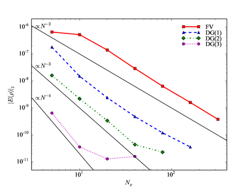
Figure 1.— Plot of the L1-norm errors in mass density for the slow magnetosonic wave perturbation test in Table 3.

4.2. Alfvén Shearing Modes

De Villiers & Hawley (2003) described a class of linear Alfvén wave solutions that test magnetic fields subject to transverse or shearing mode perturbations. Under the conditions of small amplitude perturbations with a fixed background magnetic field $B^{x}$ and constant velocity $V^{x}$ in Minkowski spacetime, the transverse velocity and field components can be written

$$V^{y}=\frac{1-\zeta\chi}{2}f(x-v_{A}^{-}t)+\frac{1+\zeta\chi}{2}f(x-v_{A}^{+}t)~{},$$ (50)

$$B^{y}=\frac{\zeta}{2}(f(x-v_{A}^{-}t)-f(x-v_{A}^{+}t))~{},$$ (51)

with

$$\zeta=\frac{B^{x}(1+\eta^{2})}{\eta\sqrt{\eta^{2}+W^{-2}}}~{},\qquad\eta^{2}=\frac{|B|^{2}}{\rho hW^{2}}~{},$$ (52)

$$\chi=-\frac{\eta^{2}V^{x}}{B^{x}(1+\eta^{2})}~{},\qquad\beta=\frac{2P}{|B|^{2}}~{},$$ (53)

and Alfvén speeds

$$v_{A}^{\pm}=\frac{V^{x}\pm\eta\sqrt{\eta^{2}+W^{-2}}}{1+\eta^{2}}~{}.$$ (54)

We consider two cases: a stationary background ($V^{x}=0$) where pulses travel in opposite directions with equal amplitudes (case ALF-1), and a moving background ($V^{x}=0.1c$) where pulses split into asymmetrical waves (case ALF-2). These cases correspond to models ALF1 and ALF3 of De Villiers & Hawley (2003). The fluid is initialized with uniform unit density, zero transverse magnetic field components $B^{y}=B^{z}=0$, specific energy $\epsilon=10^{-2}$, and ideal gas constant $\Gamma=5/3$. The longitudinal field component $B^{x}$ is set by the parameter $\beta$: 0.001 for ALF-1, 0.01 for ALF-2. The transverse velocity function $f(x,t)$ is initialized as a square pulse: $V^{y}=f(x,0)=10^{-3}c$ for $1<x<1.5$, $V^{y}=f(x,0)=-10^{-3}c$ for $1.5\leq x<2$, and zero everywhere else (the grid length runs from 0 to 3 units, with periodic boundary conditions). The Alfvén wave speeds are $|v_{A}^{\pm}|=0.96c$ for ALF-1, and $v_{A}^{+}=0.79c$ and $v_{A}^{-}=-0.71c$ for ALF-2.

Numerical results are plotted in Figure 2, where we compare analytic to DG(1) solutions. Two calculations are shown for both cases: one using entropy viscosity to capture the discontinuities, the second using the slope limiter. Solutions for the two discontinuity capturing approaches are very similar, and they both match the finite volume calculations. All solver permutations (DG, FV, viscosity, limiter) reproduce the plateau values to better than 0.002%, and converge globally to the analytic solution at rates close to unity.

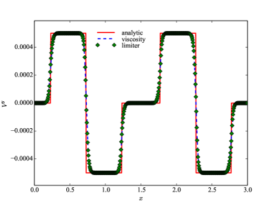
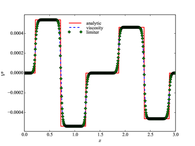
Figure 2.— Transverse velocity $V^{y}$ for the ALF-1 (left) and ALF-2 (right) shearing mode tests with 512 zone resolution. Solid lines are the analytic solutions given in the text, dashed lines are the DG(1) solutions using entropy viscosity for discontinuity capturing, and the diamonds are the DG(1) solutions with the slope limiter.

Taking advantage of the semi-analytic nature of this solution, we additionally consider a smooth wave form for the function $f(x-v_{A}^{\pm}t)=f_{0}\sin(2\pi(x-v_{A}^{\pm}t)/L)$, with small amplitude $f_{0}=10^{-8}$ to expand the perturbation regime. This allows us to perform convergence studies similar to those conducted in section 4.1. Although this problem is not as rigorous a test for hydrodynamics as those presented above, it is nonetheless a useful diagnostic of magnetically dominated flows. For these series of tests we use the 4th order, five-stage Runge-Kutta integrator and extend our testing to include DG(4), 5th order spatial discretization. L1-norm errors for $B^{y}$ are presented in Table 4 and plotted in Figure 3. As before, all calculations were run for three complete wave periods of the fast Alfvén mode. We find convergence rates generally consistent with the spatial order of each scheme: 2nd order for the FV and DG(1) schemes, and order $p+1$ for the DG($p$) methods.

Table 4L$1$-norm errors in $B^{y}$ for the smooth Alfvén shearing mode test

	$N_{x}=5$	$N_{x}=10$	$N_{x}=20$	$N_{x}=40$	$N_{x}=80$	$N_{x}=160$	$N_{x}=320$
FV	$1.0\times 10^{-8}$	$6.1\times 10^{-9}$	$3.3\times 10^{-9}$	$9.1\times 10^{-10}$	$2.3\times 10^{-10}$	$5.8\times 10^{-11}$	$1.5\times 10^{-11}$
DG(1)	$1.8\times 10^{-9}$	$6.5\times 10^{-10}$	$1.9\times 10^{-10}$	$4.9\times 10^{-11}$	$1.2\times 10^{-11}$	$3.1\times 10^{-12}$	$7.7\times 10^{-13}$
DG(2)	$3.3\times 10^{-10}$	$4.1\times 10^{-11}$	$5.2\times 10^{-12}$	$6.5\times 10^{-13}$	$8.1\times 10^{-14}$	$1.0\times 10^{-14}$
DG(3)	$2.4\times 10^{-11}$	$1.6\times 10^{-12}$	$9.8\times 10^{-14}$	$6.2\times 10^{-15}$	$3.9\times 10^{-16}$
DG(4)	$3.5\times 10^{-12}$	$1.9\times 10^{-13}$	$3.2\times 10^{-15}$	$2.6\times 10^{-16}$

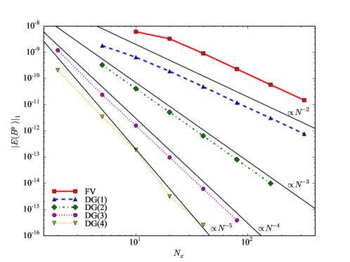
Figure 3.— Plot of the L1-norm errors in $B^{y}$ for the smooth Alfvén shearing mode perturbation test.

4.3. Hydrodynamic Shocks

We consider two special relativistic hydrodynamic shock tube tests: a relatively mild boost case (HDST-1) with $V=0.7c$, and a second higher boost case (HDST-2) with $V=0.9c$. These tests set up two different fluid states separated by a membrane in the middle of the domain that is removed at $t=0$. The fluid subsequently evolves to form a leftward propagating rarefaction wave, and rightward propagating contact discontinuity and shock wave. The initial data for HDST-1 is specified as $\rho_{L}=10$, $p_{L}=10$, $V^{x}_{L}=0$, to the left of the partition, $\rho_{R}=1$, $p_{R}=10^{-2}$, $V^{x}_{R}=0$ to the right, and a $\Gamma=4/3$ ideal gas equation of state. HDST-2 is similar but with a significantly greater pressure to the left of the membrane, $p_{L}=170$, which makes the leading Lorentz contracted density discontinuity much harder to resolve on meshes with limited cell resources.

All tests are performed separately with artificial viscosity or slope limiting, imposing flat (zero gradient) boundary conditions, and third or fourth order elements (DG(2), DG(3)) to demonstrate the robustness of the different shock regularization techniques and the application of high order finite elements to shock problems. L1-norm errors of mass density are shown in Table 5 for both cases, both regularizations, and across a range of grid resolutions to compute convergence rates. Errors are evaluated at a final time of $t=0.06$. For the viscosity runs, common values of 0.2 and 0.6 are used for the linear and quadratic coefficients respectively. The slope limiter calculations use a steepness parameter of unity. Notice that the errors quoted in Table 5 converge to the analytic solutions at roughly first order. This is what is expected for simulations that include strong discontinuities, such as shocks. The corresponding solutions are shown in Figure 4 where we plot mass densities at $t=0.15$ for HDST-1 and $t=0.08$ for HDST-2. Solid lines represent the analytic solutions derived by solving the exact Riemann problem, and dashed lines are the numerical solutions on grids resolving a domain from zero to 0.5 with 1280 zones. The numerical solutions are calculated using slope limiting in the case of HDST-1 and artificial viscosity in the case of HDST-2. In the more difficult HDST-2 test, the analytic and calculated shock jump states agree to about ten percent at the 1280 zone resolution used in producing Figure 4, but converge linearly with resolution.

Table 5L$1$-norm errors in mass density for the hydrodynamic shock tube tests

	$N_{x}=320$	$N_{x}=640$	$N_{x}=1280$	$N_{x}=2560$
HDST-1: limiter	$0.112$	$0.063$	$0.038$	$0.020$
HDST-1: viscosity	$0.105$	$0.065$	$0.043$	$0.028$
HDST-2: limiter	$0.176$	$0.105$	$0.070$	$0.038$
HDST-2: viscosity	$0.148$	$0.094$	$0.053$	$0.027$

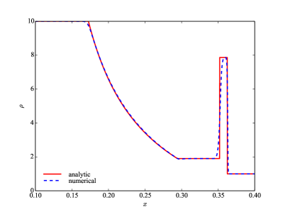
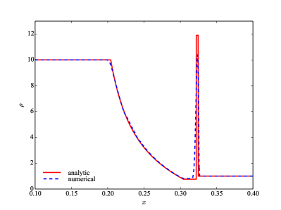
Figure 4.— Mass density $\rho$ for the hydrodynamic shock tube test HDST-1 (left) at time $t=0.15$, and HDST-2 (right) at time $t=0.08$. Solid lines are the analytic Riemann solutions and dashed lines are numerical solutions using slope limiting for shock regularization in the case of HDST-1, and artificial viscosity in the case of HDST-2. Numerical solutions are calculated on a domain from 0 to 0.5 with 1280 zones.

4.4. Boosted Shock Collision

Anninos et al. (2005) derived an exact solution for the collision of two boosted fluids that tests the Lorentz invariance of the code under rigorous non-symmetric conditions, multiple jump discontinuities, and highly relativistic shocks. In the center-of-momentum frame this problem consists of two colliding fluids, one flowing from the left, one from the right. The pre- and post-shock states of the two fluids are defined in the center of mass (primed) frame by zero post-shock velocities and pressure equilibrium assuming an infinite strength (cold fluid) approximation:

$$P_{\mathrm{post}}=\rho_{\mathrm{post}}(\Gamma-1)(W^{\prime}_{\mathrm{pre}}-1)~{},$$ (55)

$$\rho_{\mathrm{post}}=\rho_{\mathrm{pre}}\frac{1+\Gamma W^{\prime}_{\mathrm{pre}}}{\Gamma-1}~{}.$$ (56)

The observer is then boosted to the right at a specified velocity so that the shocked region appears to move to the left at very high velocities, even as they move apart (in opposite directions) in the center-of-momentum frame. The velocity of the center of mass frame and contact discontinuity is calculated by solving the nonlinear boost transformation equations. We do not repeat the derivation here, but refer the reader to Section 4.1.3 of their paper for a detailed discussion of the initialization, and their Table 2 where the solutions of three specific cases are recorded.

These tests produce highly relativistic shocks that require extremely fine zoning to properly capture the jump conditions. We achieve this with adaptive mesh refinement, using up to 7 levels of refinement on top of a base grid of length 0.06 covered by 80 zones. In addition we have run these problems with both AMR and AOR in combination to test the simultaneous use of both refinement techniques, although in practice high order polynomials are ineffective in these shock dominated cases producing results essentially identical to low order solutions. We have reproduced comparable quality solutions for all the cases derived in Anninos et al. (2005), but show representative results in Figure 5 for the case where the colliding fluids have different densities. The two fluids have initial proper densities $\rho_{1}=2$ (left), $\rho_{2}=1$ (right), pressures $P=10^{-6}$, and adiabatic index $\Gamma=5/3$. In the center of mass frame, the fluids move in opposite directions, each with $W^{\prime}=5$. The observer is boosted to the right at $W=3$, so the fluid moves at speeds up to $0.999c$. The two curves in Figure 5 are solutions for mass densities calculated with artificial viscosity shock capturing and flat boundary conditions at two different times: $t=0.01$ (dashed), and $t=0.02$ (solid), showing the shocked fluid moving to the left. The corresponding solutions with slope limiting appear very similar. For the artificial viscosity solution we find fractional density errors of $\approx 5\times 10^{-2}$ and $2\times 10^{-2}$ in the higher and lower density post-shock plateaus respectively, and energy density errors at the contact discontinuity of about $\delta e/e\approx 7\times 10^{-2}$. Errors are slightly better for the slope limiter calculations: $\delta\rho/\rho\approx 3\times 10^{-2}$ ($2\times 10^{-3}$) for the high (low) density plateaus, and $\delta e/e\approx 10^{-3}$ for the post-shock energy density.

Figure 5.— Mass density $\rho$ for the ultra-relativistic colliding shock test at two different times $t=0.01$ (solid) and 0.02 (dashed), showing the fluids moving to the left at velocity 0.999c.

4.5. MHD Shocks

Next we consider three magneto-hydrodynamic shock tube tests: the first two are taken from Komissarov (1999), the third is a relativistic version of the Brio-Wu shock tube (De Villiers & Hawley, 2003). All are initialized with zero velocities, and discontinuities separating the left and right states partitioned at the center of the grid. Additionally all three are run with the same $\Gamma=4/3$ ideal gas equation of state. Using subscripts “L” and “R” to denote left and right states, the initial data are: $\rho_{L}=1$, $P_{L}=1000$, $B^{x}_{L}=1$, $B^{y}_{L}=0$, $\rho_{R}=0.1$, $P_{R}=1$, $B^{x}_{R}=1$, $B^{y}_{R}=0$ for case MHDST-1; $\rho_{L}=1$, $P_{L}=30$, $B^{x}_{L}=0$, $B^{y}_{L}=20$, $\rho_{R}=0.1$, $P_{R}=1$, $B^{x}_{R}=0$, $B^{y}_{R}=0$ for case MHDST-2; and $\rho_{L}=1$, $P_{L}=1$, $B^{x}_{L}=0$, $B^{y}_{L}=1$, $\rho_{R}=0.125$, $P_{R}=0.1$, $B^{x}_{R}=0$, $B^{y}_{R}=-1$ for the Brio-Wu case MHDST-3.

In Table 6, we display the initial and final calculated values for each state of the shock tubes: “Left” is the initial left state, “FL” is the value at the foot of the left fast rarefaction wave, “SC” is the value at the slow compound wave, “CDL” is the left contact discontinuity, “CDR” is the right discontinuity, “FR” is the value at the foot of the right fast rarefaction fan, and “Right” is the initial right state. The numbers presented in Table 6 correspond to calculations run with artificial viscosity, but we note that results with slope limiting are similar and generally match the viscosity results to within a few percent. Like the hydrodynamic shock tube tests, these problems were run with flat boundary conditions, third order finite elements to demonstrate robustness of high order DG on magnetized shock problems. Representative solutions of the mass density calculated on a 1024 zone grid are plotted in Figure 6 showing results from all three tests.

Table 6Initial and final state solutions for the MHD shock tube tests

	Variable	Left	FL	SC	CDL	CDR	FR	Right
MHDST-1:	$\rho$	1.0	0.07	…	0.69	…	…	0.1
MHDST-1:	$P$	1000	28.5	…	…	…	…	1.0
MHDST-2:	$\rho$	1.0	0.24	…	0.63	…	…	0.1
MHDST-2:	$P$	30.	4.6	…	15.5	…	…	1.0
MHDST-3:	$\rho$	1.0	0.51	0.67	0.55	0.35	0.11	0.125
MHDST-3:	$P$	1.0	0.41	0.59	0.45	0.45	0.08	0.1

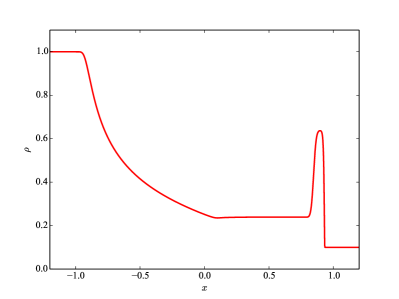
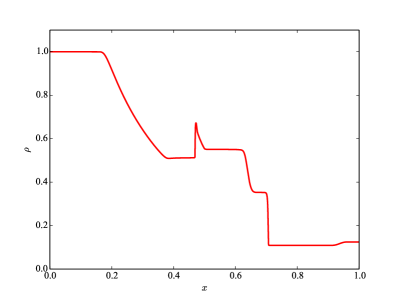
Figure 6.— Mass density $\rho$ for the three relativistic MHD shock tube tests using artificial viscosity shock regularization and 1024 zones. Solutions are plotted at times $t=1$, 1, and 0.5 for the MHDST-1, -2, and -3 cases, respectively.

4.6. Orszag-Tang

The Orszag-Tang vortex problem (Orszag & Tang, 1979) has become a standard test of magnetic fields and divergence conservation. Numerous solutions exist in the literature to which we can compare our results. In particular we follow and adopt initial data from Sa̧dowski et al. (2014) and Mocz et al. (2014): uniform density $\rho=\Gamma^{2}/(4\pi)$, pressure $P=\Gamma/(4\pi)/{\cal C}^{2}$, velocity $V^{i}=[-\sin(2\pi y),~{}\sin(2\pi x),~{}0]/{\cal C}$, magnetic field $B^{i}=[-\sin(2\pi y),~{}\sin(4\pi x),~{}0]/\sqrt{4\pi}/{\cal C}$, adiabatic index $\Gamma=5/3$, and a scale factor ${\cal C}=100$. The problem is evolved out to a time of $t=50$, on a $256\times 256$ unit two dimensional grid $0\leq(x,y)\leq 1$ with periodic boundary conditions applied in both directions. Figure 7 shows the mass density and divergence error at the final time using third order DG(2) finite elements. Also shown in Figure 8 is a horizontal line out of the density multiplied by $4\pi$ along $y=0.75$, $4\pi\rho(x,y=0.75)$. Both figures can be compared to the corresponding results from Figure 4 of Sa̧dowski et al. (2014) and Figure 16 of Mocz et al. (2014). Agreement is excellent considering the solutions in Sa̧dowski et al. (2014) and Mocz et al. (2014) were calculated on greater $640\times 640$ and $512\times 512$ resolution grids respectively. In addition, we find global normalized divergence errors $|\partial_{i}B^{i}|\Delta\ell/\sqrt{P_{B}}$ comparable to those reported by Mocz et al. (2014): roughly a few $\times 10^{-3}$ that plateau early and remain constant through most of the simulation.

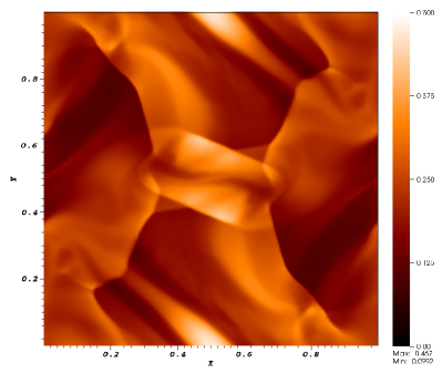
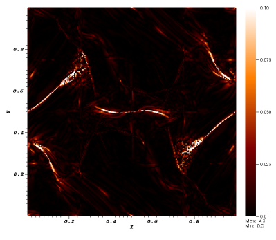
Figure 7.— Mass density (left) and divergence error (right) in the Orszag-Tang vortex test. Images are shown at the final time $t=50$ calculated on a $256\times 256$ grid using third order finite elements.

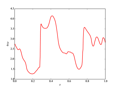
Figure 8.— Mass density multiplied by $4\pi$ as extracted along the horizontal line $y=0.75$ from Figure 7.

4.7. Kelvin-Helmholtz Instability

In this section we present convergence studies of the linear growth phase of the two-dimensional magnetized Kelvin-Helmholtz instability (KHI). Following interesting observations by Mignone et al. (2009) on the performance of various Riemann solvers in this class of problems, Beckwith & Stone (2011) published a brief study of KHI turbulence that provides a useful test of high order adaptive numerical methods, so we attempt to duplicate some of their findings here. The problem consists initially of two oppositely traveling $\Gamma=4/3$ fluids in pressure equilibrium $P=1$, densities $\rho=1$ and $10^{-2}$, and the following velocity profiles:

$$V^{x}=-V_{\mathrm{shear}}\tanh\left(\frac{y-y_{0}}{a}\right)~{},$$ (57)

$$V^{y}=-A_{0}V_{\mathrm{shear}}~{}\sin(2\pi x)~{}\exp\left(-\left(\frac{y-y_{0}}{\sigma}\right)^{2}\right)~{},$$ (58)

with shear velocity $V_{shear}=0.5$, perturbation amplitude $A_{0}=0.1$, shear layer thickness $a=0.01$, characteristic length scale $\sigma=0.1$, and interface position $y_{0}=L_{y}/2$ where $L_{y}$ is the grid length along the $y$ axis. The density is linearly interpolated similar to the shear velocity $V^{x}$ profile along the $y$-axis so that $\rho=1$ in regions with $V^{x}=0.5$ and smoothly extended to $\rho=10^{-2}$ in regions with $V^{x}=-0.5$. A single component magnetic field is introduced aligned along the $x$-direction with $B^{x}=10^{-3}$. In addition, one percent Gaussian perturbations are applied to both $x$ and $y$ components of the velocity, modulated by the same exponential damping function used in equation (58). The computation domain covers $0\leq(x,y)\leq 1$, and for the AMR calculations is resolved with a base grid of $64\times 64$ cells. Periodic (reflection) boundary conditions are enforced along the $x$($y$)-axis. Three or four additional levels of mesh refinement are applied to capture the fluid interface at effective $512\times 512$ or $1024\times 1024$ resolutions, adaptively refining (and de-refining) on the dimensionless slope of the mass density. The threshold refinement (derefinement) criteria for all cases is set to $s_{r}$ = 0.05 (0.001), where $s_{r}=|\ell^{i}\partial_{i}\rho|/\overline{\rho}$, $\ell^{i}$ is a vector of cell widths in each spatial dimension, and $\overline{\rho}$ is the local (nearest neighbor) average of the mass density.

A good diagnostic of the linear growth stage of the KHI is the temporal history of the square of the transverse four-velocity weighted by cell volume and averaged over the entire grid, $<|u^{y}|^{2}>$. This quantity is plotted in Figure 9 for four cases: KHFV representing the converged second order finite volume solution, KHDG1-3L using second order DG(1) with 3 AMR levels, KHDG1-4L using DG(1) with 4 AMR levels, and KHDG2-512 using third order DG(2) (both adaptive and fixed polynomial order) on a uniform $512\times 512$ mesh. The finite volume calculation (KHFV, solid line) reproduces converged results from Beckwith & Stone (2011), matching the slope, magnitude, and peak position in time. These four calculations collectively demonstrate convergence towards the resolved solution with both mesh and basis order refinement. Notice in particular that run KHDG1-4L (second order with 4 AMR levels, or effectively $1024\times 1024$ resolution across the interface) is nearly identical to the result of KHDG2-512 (third order with $512\times 512$ resolution), and that both significantly improve compared to the lowest resolution result KHDG1-3L (second order with 3 AMR levels).

The density distribution is shown in Figure 10 at time $t\approx 3.3$ using the DG(1) method on a single $1024\times 1024$ grid. Interestingly, this calculation exhibits signs of a developing secondary vortex at $x\approx 0.25$ that is not present in second order calculations with resolutions less than $1024\times 1024$. Similar features however are observed at lower resolutions provided high order (greater than second) finite element representations are utilized. The third order KHDG2-512 calculation, for example, produces a similar feature at $512\times 512$ resolution. Sensitivities associated with the development of a secondary vortex have been observed by Mignone et al. (2009) and Beckwith & Stone (2011) who attributed this behavior to the accuracy of the Riemann solver and its ability to capture the contact discontinuity. That DG evolves this feature with a 2-speed HLL Riemann solver with no contact steepening is encouraging and represents yet another potential benefit of the DG methodology.

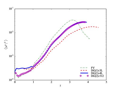
Figure 9.— Volume averaged transverse four-velocity $\langle|u^{y}|^{2}\rangle$ as a function of time over the linear growth phase of the magnetized Kelvin-Helmholtz instability. The dot-dashed line corresponds to a converged finite volume solution (case KHFV) resembling very closely the results from Beckwith & Stone (2011), including slope, magnitude, and peak location. The remaining curves represent the DG(1) solution with 3 AMR levels (case KHDG1-3L, dashed line), DG(1) with 4 AMR levels (case KHDG1-4L, solid line), and DG(2) on a single $512\times 512$ grid (run KHDG2-512, circles).

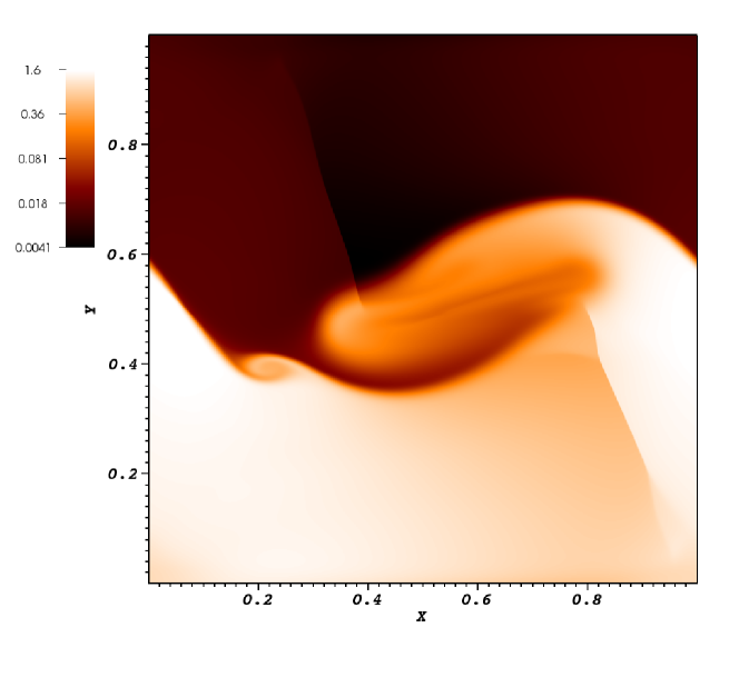
Figure 10.— Log of the mass density in the magnetized Kelvin-Hemholtz instability test shown at time $t\approx 3.3$ using the DG(1) method on a single $1024\times 1024$ grid.

4.8. Bondi Accretion

A popular test with general relativistic spacetime curvature source terms is radial accretion onto a compact Schwarzschild black hole. The analytic solution is characterized by a critical point $r_{c}$ in the flow (Michel, 1972)

$$(u_{c}^{r})^{2}=\frac{M}{2r_{c}}~{},$$ (59)

$$v_{c}^{2}=\frac{(u_{c}^{r})^{2}}{1-3(u_{c}^{r})^{2}}=\frac{(1+n)T_{c}}{n(1+(1+n)T_{c})}~{},$$ (60)

where $u_{c}^{r}$ and $v_{c}$ are the radial 4-velocity and sound speed at the critical point, respectively, $M$ is the black hole mass, $n=1/(\Gamma-1)$ is the polytropic index, and $T=P/\rho$ is the fluid temperature. The solution is completed with the following parametrization

$$T^{n}u^{r}r^{2}=C_{1}~{},$$ (61)

$$(1+(1+n)T)^{2}~{}\left(1-\frac{2M}{r}+(u^{r})^{2}\right)=C_{2}~{}.$$ (62)

The constants $C_{1}$ and $C_{2}$ are fixed by choosing the critical radius $r_{c}=8GM/c^{2}$, setting $\Gamma=4/3$, and defining the mass density at the critical radius ($\rho_{c}$) by setting the mass accretion rate to $\dot{M}=4\pi r_{c}^{2}\rho_{c}u^{r}_{c}=-1$.

We choose spherical Kerr-Schild coordinates for this test to cover a two-dimensional computational domain bounded in radius from $r=0.98r_{BH}$ to $r=20GM/c^{2}$, where $r_{BH}=2GM/c^{2}$ is the radius of the black hole horizon. The angular extent is a thin wedge centered along the equatorial symmetry axis of width $\Delta\theta=\pi/20$. The Bondi solution is initialized from the outset at $t=0$ then evolved over a time interval of $5GM/c^{2}$. Constant boundary conditions consisting of the analytic solution are imposed at the inner and outer radial boundaries, and symmetric boundaries are enforced in the angular coordinate. Accuracy and convergence are evaluated by calculating L1-norm errors in density between initial and final times along the equatorial plane over the entire radial extent of the grid. Although CosmosDG supplies analytic metric gradients for many black hole metric representations, for this test we instead evaluate gradients numerically in order to test our implementation of finite element gradient operators. A series of nine calculations were performed with three DG orders (2nd, 3rd, 4th) and three grid resolutions: $N_{r}\times N_{\theta}=$ $16\times 2$, $32\times 4$, $64\times 8$, where $N_{r}$ and $N_{\theta}$ are the number of zones along the radial and angular directions. All calculations were run with 4th order time integration using the 5-stage Runge-Kutta method. Like previous smooth field tests, we find DG methods produce significantly smaller evolution errors than FV, an order of magnitude or more depending on the basis order, and converge to the analytic solution at the appropriate rate. For example, FV produces L1-norm errors of $3.8\times 10^{-4}$ in mass density computed on a $64\times 8$ grid. Equivalent errors from DG(1), DG(2) and DG(3) methods come to $1.5\times 10^{-4}$, $1.3\times 10^{-5}$ and $1.2\times 10^{-7}$ respectively. In addition we find with each doubling of zones, errors are reduced by factors of about $2^{p+1}$ for methods DG($p$) as expected and as demonstrated in Table 7 and Figure 11.

This hydrodynamic black hole accretion test can be adapted to include a radial magnetic field satisfying $\partial_{r}B^{r}=0$ and which does not alter the analytic solution for any of the primitive fields ($\rho$, $p$ or $u^{r}$). Although this treatment does not satisfy the full Maxwell equations (Antón et al., 2006), it is a useful nontrivial test of magnetic fields in the code. We set the magnitude of the magnetic field by $|b|^{2}/\rho=10.56$ at the critical point, effectively equating hydrodynamic and magnetic pressures at $r=r_{c}$. Performing equivalent calculations (identical grids, resolutions, fluid and black hole parameters) as the hydrodynamic version, we find errors similar to those presented in Table 7.

Table 7L$1$-norm errors in $\rho$ for the Bondi accretion test

	$16\times 2$	$32\times 4$	$64\times 8$
DG(1)	$3.1\times 10^{-3}$	$6.5\times 10^{-4}$	$1.5\times 10^{-4}$
DG(2)	$6.1\times 10^{-4}$	$9.5\times 10^{-5}$	$1.3\times 10^{-5}$
DG(3)	$3.3\times 10^{-5}$	$1.7\times 10^{-6}$	$1.2\times 10^{-7}$

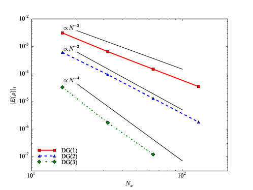
Figure 11.— Plot of the L1-norm errors in $\rho$ for the Bondi accretion test.

4.9. Magnetized Black Hole Torus

For a final test we expand on the Bondi accretion problem and consider a magnetized torus of gas orbiting around a rotating black hole. There is no analytic solution for this problem so in its place we instead compare a DG finite element solution against a comparable finite volume calculation. Like the Bondi test we use spherical Kerr-Schild spacetime coordinates, but set the spin of the black hole to $a/M=0.9$, the specific angular momentum of the torus to $\ell/M=4.3$, and the surface potential to $(u_{t})_{in}=-0.98$, producing a torus of mass $M_{torus}=1390M$ orbiting in rotational equilibrium around the central potential of the black hole. The background regions are initially set to be cold ($e=10^{-6}e_{\text{max}}$), low density ($\rho=10^{-6}\rho_{\text{max}}$), and static ($V^{i}=0$), where $e_{\text{max}}$ and $\rho_{\text{max}}$ are the internal energy density and mass density at the pressure maximum of the torus located at radius $r_{\text{cent}}=15.3GM/c^{2}$. The orbital period at $r_{\text{cent}}$ is $t_{orb}=380GM/c^{3}$. The torus is set up with a polytropic constant $\kappa=0.01$ and (along with the background gas) obeys an ideal gas equation of state with adiabatic index $\Gamma=5/3$.

In order to seed the magnetorotational instability (MRI), the torus is threaded initially with a weak poloidal magnetic field derived from the following vector potential:

$$A_{\phi}=\begin{cases}k(\rho-\rho_{\text{cut}})&\text{if}\quad\rho>\rho_{\text{cut}}~{},\\ 0&\text{otherwise}~{},\end{cases}$$ (63)

where $\rho_{\text{cut}}=0.5\rho_{\text{max}}$ effectively keeps the magnetic field inside the torus surface. The field is normalized by defining the constant $k$ so that $\beta=P/P_{B}\geq 2$ throughout the torus. Although initially confined to the torus, eventually the field evolves to fill most of the background with a magnetized corona and high-$\beta$ outflows, in addition to seeding the MRI and launching an accretion flow from the torus to the black hole. It is this accretion flow that we use as a diagnostic for comparing results from the different numerical methods.

This problem is run on a two-dimensional, azimuthally symmetric grid resolved effectively with $128\times 128$ cells: The finite volume calculation representing the “known” solution is run on a single $128\times 128$ grid, while the finite element calculations on a 2-level nested grid with $64\times 64$ base resolution to demonstrate simultaneous use of hierarchical mesh and basis order refinement. We typically simulate accretion disks in this mode (with nested grids) to achieve greater resolution along the equatorial plane while simultaneously avoiding refining along the pole-axis to relax the Courant constraint. However, we have verified that replacing nested grids with fully adaptive mesh refinement produces similar results. We also use a logarithmic radial coordinate of the form $\eta=1+\ln(r/r_{\text{BH}})$ and a concentrated angular coordinate $x_{2}$ such that $\theta=x_{2}+\sin(2x_{2})/4$ to further increase the resolution near the black hole horizon and along the equator. The grid covers $0.1\pi\leq\theta\leq 0.9\pi$ and $0.98r_{\text{BH}}\leq r\leq 120M$, resulting in cell widths of $\Delta r\approx 0.05GM/c^{2}$ near the inner radial boundary and $\Delta r\approx 0.5GM/c^{2}$ near the initial pressure maximum of the torus. By comparison, the characteristic wavelength of the MRI is $\lambda\equiv 2\pi v_{A}/\Omega\approx 2.5GM/c^{2}$ near the initial maximum. Symmetric (reflective) boundary conditions are imposed along the radial (angular) directions.

Our comparison is between a traditional finite volume with piecewise parabolic reconstruction (case BHT-FV) and an adaptive-order-refinement using second-order finite elements in the background gas and third order in the torus body (case BHT-DG2), refining and derefining the polynomial order on the gas density (refining when the density exceeds 0.0005, derefining when density drops below 0.0001). Figures 12 and 13 show images of the logarithmic gas density, comparing BHT-FV and BHT-DG2 solutions at two different times in the evolutions. The left images correspond to an early time when the torus stream first hits the horizon. The right images show a later snapshot when the flow has fully developed after a couple of orbits. Figure 14 compares mass accretion rates as a function of time for each of the cases. We expect differences due to the turbulent nature of these calculations, but the level of differences between the methods appears significant, paying particular attention to the temporal variability of the mass accretion, the duration of the flow period before it begins to taper off, and the total accreted mass (about 12% and 19% of the initial torus mass after five orbits for cases BHT-FV and BHT-DG2, respectively). These results are consistent with previous similar calculations (Anninos et al., 2005), though we note the slightly greater total accreted mass for the finite element calculation. More exhaustive studies of black hole accretion will be conducted in future work to understand better the accuracy and benefits of high order methods for capturing sub-zonal effects. Here we have taken the first step towards this goal, validating the DG finite element methodology and demonstrating its utility to this class of problems.

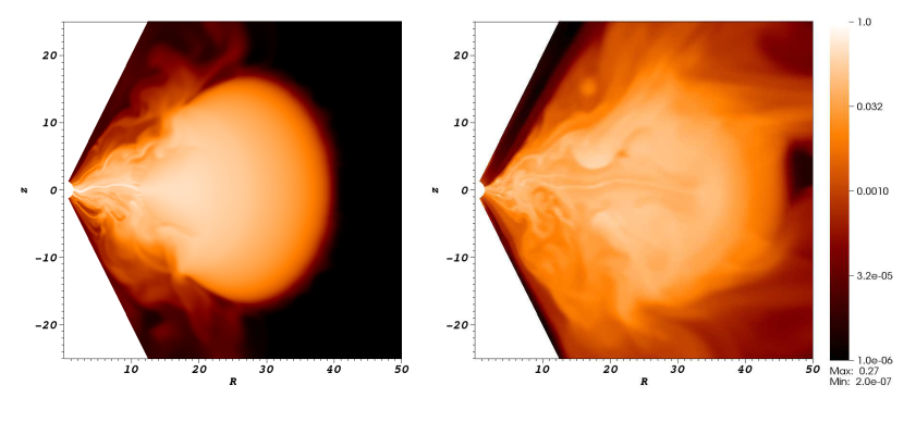
Figure 12.— Log of the mass density in the magnetized black hole torus accretion test calculated with the finite volume method. The left image corresponds to $t=199$ ($0.5~{}t_{orb}$), and the right to $t=760$ ($2~{}t_{orb}$).

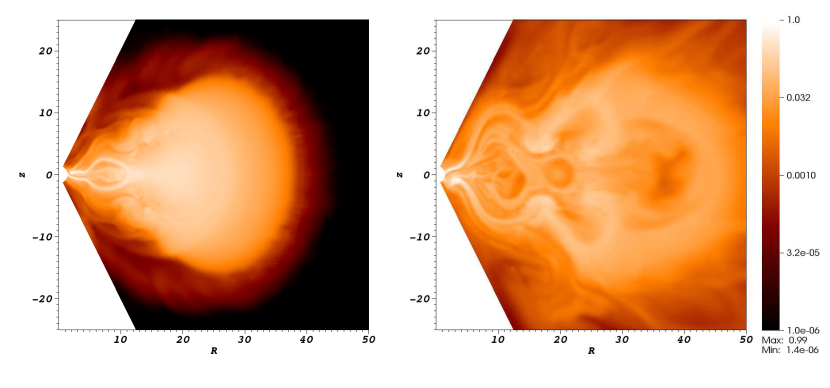
Figure 13.— Log of the mass density in the magnetized black hole torus accretion test calculated with the adaptive third order DG finite element method. The left image corresponds to $t=199$ ($0.5~{}t_{orb}$), the right to $t=760$ ($2~{}t_{orb}$).

Figure 14.— Mass accretion rates $\dot{M}$ across the inner radial boundary, comparing the finite volume (case BHT-FV, top) and adaptive, third-order finite element (case BHT-DG2, bottom) solutions.

5. Discussion

We have developed a new version of Cosmos++, called CosmosDG, a code for both Newtonian and general relativistic radiation magnetohydrodynamics, based on the Discontinuous Galerkin (DG) finite element formulation. The code infrastructure in CosmosDG was upgraded to accommodate simultaneous use of cell-by-cell adaptive mesh refinement (AMR) together with cell-by-cell adaptive basis order refinement (AOR). Our current implementation utilizes Lagrange interpolatory functions to construct local finite element approximations of arbitrary spatial order, with multiple options for high order time integration, including 3rd order forward Euler, and 4th order strong stability preserving Runge-Kutta. Generalization to two and three dimensions is accomplished through tensor products of one-dimensional basis functions. Although our DG implementation can construct basis polynomials of arbitrary order, in practice we find that 3rd or 4th order is a practical upper limit set by computational speed and saturation of errors due to machine precision constraints.

Two options are provided for the regularization of shock discontinuities: artificial viscosity and/or slope limiters (they can be invoked separately or together). Artificial viscosity is applied in a conservative manner using covariant Laplacian smoothing operators with properly normalized entropy or relativistic enthalpy diagnostics to trigger the application of viscosity locally when cell interface jumps or excessive sub-zonal heating are detected. The slope limiter option is a modification of the traditional minmod limiter commonly used in finite volume and finite difference codes, generalized here to work in multi-dimensions and for arbitrary order finite elements by projecting high order solutions to a low order basis using a least squares method to compute slopes. Both approaches were demonstrated to provide adequate stabilization of shocks, for all polynomial orders. We note that artificial viscosity is implemented as sub-zonal dissipation terms, preserving the high order nature of DG($p$) in each cell. Slope limiting, however, is currently applied across zone interfaces like traditional finite volume methods, effectively folding high order sub-grid data into second order solutions before enforcing monotonicity. We are currently investigating a number of approaches for extending slope limiting to work directly on unfiltered sub-grid data.

We demonstrated the ability of DG finite element methods to achieve arbitrarily high order convergence on perturbation problems with smooth profiles (i.e., sonic and magnetosonic waves), limited only by analytic solution and machine precision limits. Our extensive testing of DG methods furthermore proved them equal to or, in most cases, better than finite volume methods, using high resolution shock capturing or central difference schemes, even for problems with highly relativistic shocks, regimes with strong discontinuities where high order can break down and lead to unwanted Gibbs effects. Perhaps more importantly we have subjected this methodology to the rigors of multi-dimensional modeling of energetic astrophysical environments, complex hydrodynamic instabilities, and strong spacetime curvature, successfully demonstrating its application to Bondi-Hoyle and MRI-induced black hole accretion.

References

- Anninos & Fragile (2003) Anninos, P., & Fragile, P. C. 2003, ApJS, 144, 243
- Anninos et al. (2003) Anninos, P., Fragile, P. C., & Murray, S. D. 2003, ApJS, 147, 177
- Anninos et al. (2005) Anninos, P., Fragile, P. C., & Salmonson, J. D. 2005, ApJ, 635, 723
- Antón et al. (2006) Antón, L., Zanotti, O., Miralles, J. A., Martí, J. M., Ibáñez, J. M., Font, J. A., & Pons, J. A. 2006, ApJ, 637, 296
- Babus̆ka et al. (1986) Babus̆ka, I., Zienkiewicz, O. C., Gago, J., & de A. Oliveira, E. R., eds. 1986, Accuracy Estimates and Adaptive Refinements in Finite Element Computations (John Wiley and Sons, Chichester)
- Beckwith & Stone (2011) Beckwith, K., & Stone, J. M. 2011, ApJS, 193, 6
- Cockburn et al. (1989) Cockburn, B., Lin, S.-Y., & Shu, C.-W. 1989, Journal of Computational Physics, 84, 90
- Cockburn & Shu (1989) Cockburn, B., & Shu, C.-W. 1989, Mathematics of Computation, 52, 411
- Cockburn & Shu (1998) —. 1998, Journal of Computational Physics, 141, 199