Entanglement dynamics in de Sitter spacetime

Abstract

We apply the master equation with dynamical coarse graining approximation to a pair of detectors interacting with a scalar field. By solving the master equation numerically, we investigate evolution of negativity between comoving detectors in de Sitter space. For the massless conformal scalar field with the conformal vacuum, it is found that a pair of detectors can perceive entanglement beyond the Hubble horizon scale if the initial separation of detectors is sufficiently small. At the same time, violation of the Bell-CHSH inequality on the super horizon scale is also detected. For the massless minimal scalar field with the Bunch-Davies vacuum, on the other hand, the entanglement decays within Hubble time scale owing to the quantum noise caused by particle creations in de Sitter space and the entanglement on the super horizon scale cannot be detected.

I Introduction

The entanglement is one of the most important quantity in the quantum mechanics and quantum information Nielsen2007 . In the context of the inflationary scenario, investigating nature of entanglement for quantum fields in de Sitter spacetime is crucial to understand mechanism of quantum to classical transition of primordial fluctuation generated during inflation Nambu2008 ; Nambu2009 ; Nambu2011 ; Nambu2013 . This subject is also expected to reveal the relation between causal structures of spacetime and quantum information. In cosmological situation, the particle detector model Unruh1976a ; DeWitt1979 ; Birrell1984 is applied to study nature of entanglement of quantum fields. In de Sitter space, with the lowest order perturbation calculation, it was shown that detection of entanglement of the quantum field is possible when a separation of a pair of detectors is smaller than $2H^{-1}$ for the massless conformal scalar field with the conformal vacuum and $0.6H^{-1}$ for the minimal massless scalar field with the Bunch-Davies vacuum Steeg2009 ; Nambu2011 ; Nambu2013 ; Martin-Martinez2014 . To investigate time evolution of entanglement between detectors, perturbative calculation is limited due to appearance of the secular behavior and it is only possible to discuss initial detection of entanglement within short time scales.

To explore long time dynamics of detectors, a method featuring an open quantum system can be applied Breuer2002 : By taking partial trace of degrees of freedom of the quantum field as a bath (environment), the dynamics of the detector system is derived as a quantum master equation. In general, the master equation becomes an integro-differential equation, and the state at the specific time depends on its past evolution (i.e. it is non-Markovian nature). However, it is possible to recover the Markovian property of the master equation by assuming that the bath time scale is sufficiently shorter than the relaxation time scale of the system. By combining this assumption with so-called the secular approximation (rotation wave approximation), which neglects transition via non-energy-conversing processes, it can be shown that the resulting master equation has the Gorni-Kossakowski-Lindblad-Sudarshan (GKLS) Gorini1976 ; Lindblad1976 form, and preserves the trace and the complete positivity of the state in course of time evolution.

Many authors have applied the quantum master equation to explore physics of quantum field in curved spacetimes. A single detector system was investigated to study thermalization by the Hawking radiation and the Unruh effect  Yu2008 , and a two detectors system was applied to investigate the dynamics of the entanglement for Unruh effect Hu2013 ; Tian2014 ; Hu2015 ; Tian2016 . In these previous studies, analyses are relied on the master equations with the secular approximation. However, this approximation can not be applied when the state of the bath is not time translational invariant because the meaning of energy conservation of the total system is unclear in such a case. Hence, it is not suitable to apply the master equation with the secular approximation in cosmological situations. As an alternative to the secular approximation, the dynamical coarse graining (DCG) approximation was proposed recently Lidar2001 ; Schaller2008 ; Benatti2010 ; Majenz2013 ; Nambu2016a . The master equation under this approximation also satisfies the complete positivity and the Markovian property. It contains a free parameter $\Delta$ which specifies the coarse graining time scale, and reduces to the master equation with the secular approximation in the limit $\Delta\rightarrow\infty$. By its definition, this master equation can be applied to the environment with no time translation invariance such as a quantum field in de Sitter spacetime, provided that the coarse graining time scale is chosen to be sufficiently shorter than the Hubble time scale.

To investigate entanglement between two detectors in cosmological situation, papers Hu2013 ; Tian2014 applied the master equation with the secular approximation. They considered the massless conformal scalar field in de Sitter spacetime with a static chart and examined how two static detectors can perceive entanglement of the quantum field. Due to the Unruh effect and the Hawking radiation in de Sitter spacetime, they concluded that the entanglement detected has different behavior from that of the thermal field with Hawking temperature given by the Hubble parameter in de Sitter space. In their setting, the entanglement beyond the Hubble horizon can not be evaluated. Thus, it is interesting to investigate how the initial detected entanglement is affected by quantum noise in de Sitter spacetime after horizon exit. In this paper, we aim to discuss whether the entanglement between comoving detectors persist beyond the Hubble horizon. For this purpose, we apply a method of the master equation with DCG approximation to two comoving detectors interacting with a scalar field in de Sitter space. We assume two detectors are initially prepared to be separable and trace evolution of detectors’ quantum state.

The structure of this paper is as follows. In Section II, we introduce the master equation with DCG approximation and our detector model. In Section III, we introduce test of the Bell-CHSH inequality in our set up of detectors model. Then, in Section IV, we investigate the evolution of the entanglement between two detectors using the master equation. Section V is devoted to summary.

II Master equation of detector model

II.1 Master equation with dynamical coarse-graining approximation

We introduce the quantum master equation with the dynamical coarse graining approximation Lidar2001 ; Schaller2008 ; Benatti2010 ; Majenz2013 . We basically follow the presentation by Benatti et al. Benatti2010 . The total Hamiltonian is composed of detector variables (system) interacting with quantum scalar fields (bath). The total Hamiltonian is

$$H=H_{0}^{S}+H_{0}^{B}+\lambda V,$$ (1)

where $H_{S}$ is the system Hamiltonian and $H_{B}$ is the bath Hamiltonian and $V=\sum_{A}\sigma_{A}\Phi_{A}$ is the interaction Hamiltonian, where $\sigma_{A}$ is the system operator and $\Phi_{A}$ is the bath field. $\lambda$ represents a coupling constant and we assume that interaction between the system and the bath is small $\lambda\ll 1$ (weak coupling limit). The total density operator $\rho_{T}(t)$ in the Schrödinger picture obeys the von Neumann equation

$$\frac{d\rho_{\text{T}}(t)}{dt}=-i[H_{0}+\lambda V,\rho_{\text{T}}(t)],\quad H_{0}=H_{0}^{\text{S}}+H_{0}^{\text{B}}.$$ (2)

Our purpose is to obtain an equation for the reduced density operator for detector system

$$\rho(t)\equiv\mathrm{Tr}_{\text{B}}\{\rho_{\text{T}}(t)\}.$$ (3)

In the interaction picture, the state is

$$\tilde{\rho}_{\text{T}}(t)=U(t;t_{0})^{\dagger}\rho_{\text{T}}(t)U(t;t_{0}),$$ (4)

where $U(t;t_{0})$ is the time evolution operator by the free Hamiltonian $H_{0}$

$$U(t;t_{0})={\cal T}\exp\{-i\int^{t}_{t_{0}}H_{0}\,dt^{\prime}\},$$ (5)

and ${\cal T}$ denotes the time ordering operator.

Then, $\tilde{\rho}_{\text{T}}(t)$ obeys

$$\frac{d\tilde{\rho}_{\text{T}}}{dt}=-i[\lambda\tilde{V}(t),\tilde{\rho}_{\text{T}}],\quad\tilde{V}(t)=U(t;t_{0})^{\dagger}VU(t;t_{0}).$$ (6)

The solution of the above equation up to the second order of the perturbation is

$$\tilde{\rho}_{\text{T}}(t) =\tilde{\rho}_{\text{T}}(t_{0})-i\lambda\int_{t_{0}}^{t}dt_{1}\,[\tilde{V}(t_{1}),\tilde{\rho}_{\text{T}}(t_{0})]$$

$$-\lambda^{2}\int_{t_{0}}^{t}dt_{1}\int_{t_{0}}^{t_{1}}dt_{2}\,[\tilde{V}(t_{1}),[\tilde{V}(t_{2}),\tilde{\rho}_{\text{T}}(t_{0})]]+O(\lambda^{3}).$$ (7)

We assume that during evolution, the state of the total system is a product state

$$\tilde{\rho}_{\text{T}}(t)\approx\tilde{\rho}(t)\otimes\rho_{B}.$$ (8)

where $\rho_{B}=\rho_{B}(t_{0})$. This assumption is justified because the interaction between the system and the bath is weak and the correlation between the system and the bath can be neglected when the bath time scale is shorter than the system time scale. By taking the trace of the perturbative solution (7) with respect to the bath degrees of freedom,

$$\tilde{\rho}(t)=\tilde{\rho}(t_{0})-\lambda^{2}\int_{t_{0}}^{t}dt_{1}\int_{t_{0}}^{t_{1}}dt_{2}{\mathrm{Tr}}_{B}[\tilde{V}(t_{1}),[\tilde{V}(t_{2}),{\rho}(t_{0})\otimes{\rho}_{B}(t_{0})]],$$ (9)

where we have assumed $\langle\Phi_{A}\rangle$=0. After rewriting (9),

$$\tilde{\rho}(t)-\tilde{\rho}(t_{0})=\Delta\times\left(-i[H_{12},\rho_{0}]+\mathcal{L}[\rho_{0}]\right),\quad\Delta=t-t_{0},\quad\rho_{0}=\rho(t_{0}),$$ (10)

and we have defined

$$H_{12} =-i\frac{\lambda^{2}}{2\Delta}\sum_{A_{1}A_{2}}\int_{0}^{\Delta}ds_{1}\int_{0}^{\Delta}ds_{2}\,\mathrm{sgn}(s_{1}-s_{2})\,G_{A_{1}\!A_{2}}(s_{1}-s_{2})\sigma_{A_{1}}(s_{1}+t_{0})\sigma_{A_{2}}(s_{2}+t_{0}),$$ (11)

$$\mathcal{L}[\rho_{0}] =\frac{\lambda^{2}}{\Delta}\sum_{A_{1}A_{2}}\int_{0}^{\Delta}ds_{1}\int_{0}^{\Delta}ds_{2}\,G_{A_{1}\!A_{2}}(s_{1}-s_{2})\left(\sigma_{A_{2}}(s_{2}+t_{0})\rho_{0}\sigma_{A_{1}}(s_{1}+t_{0})-\frac{1}{2}\{\sigma_{A_{1}}(s_{1}+t_{0})\sigma_{A_{2}}(s_{2}+t_{0}),\rho_{0}\}\right),$$ (12)

where the bath correlation function is introduced by

$$G_{A_{1}\!A_{2}}(t_{1}-t_{2})=\mathrm{Tr}_{B}\{\Phi_{A_{1}}(t_{1})\Phi_{A_{2}}(t_{2})\rho_{B}(t_{0})\}=\langle\Phi_{A_{1}}(t_{1})\Phi_{A_{2}}(t_{2})\rangle.$$ (13)

The time dependence of the system variable can be written as

$$\sigma_{A}(t)=\sum_{B}u_{AB}(t-t_{0})\sigma_{B},\quad u_{AB}(0)=1,$$ (14)

where the specific form of the function $u_{AB}(t)$ depends on the system Hamiltonian. Using this relation, we obtain

$$H_{12} =\sum_{B_{1}B_{2}}H_{B_{1}\!B_{2}}\sigma_{B_{1}}\sigma_{B_{2}},$$ (15)

$$\mathcal{L}[\rho_{0}] =\sum_{B_{1}B_{2}}C_{B_{1}\!B_{2}}\left(\sigma_{B_{2}}\rho_{0}\,\sigma_{B_{1}}-\frac{1}{2}\{\sigma_{B_{1}}\sigma_{B_{2}},\rho_{0}\}\right),$$ (16)

with

$$H_{B_{1}\!B_{2}}=-i\frac{\lambda^{2}}{2\Delta}\sum_{A_{1}A_{2}}\int_{0}^{\Delta}ds_{1}\int_{0}^{\Delta}ds_{2}\,\mathrm{sgn}(s_{1}-s_{2})\,G_{A_{1}\!A_{2}}(s_{1}-s_{2})u_{A_{1}\!B_{1}}(s_{1})u_{A_{2}\!B_{2}}(s_{2}),$$ (17)

$$C_{B_{1}\!B_{2}}=\frac{\lambda^{2}}{\Delta}\sum_{A_{1}A_{2}}\int_{0}^{\Delta}ds_{1}\int_{0}^{\Delta}ds_{2}\,G_{A_{1}\!A_{2}}(s_{1}-s_{2})\,u_{A_{1}\!B_{1}}(s_{1})u_{A_{2}\!B_{2}}(s_{2}).$$ (18)

As $t_{0}$ is an arbitrary initial time in Eq. (9), it is possible to convert (9) to the master equation by assuming that the bath time scale is shorter than the system time scale, and the interaction is weak Benatti2010 ; Nambu2016a . In the Schrödinger picture,

$$\frac{d}{dt}\rho=-i[H_{\text{eff}},\rho]+\mathcal{L}[\rho],\quad H_{\text{eff}}=H_{0}^{S}+H_{12}.$$ (19)

This is the master equation with dynamical coarse-graining approximation and has the GKLS form. This time scale of coarse graining is specified by the parameter $\Delta$. It can be shown that the coefficients $C_{B_{1}\!B_{2}}$ in $\mathcal{L}[\rho]$ form a positive matrix. Thus, this master equation preserves the trace and the complete positivity of the state. In the limit of $\Delta\rightarrow\infty$, (19) reduces to the master equation with the secular approximation.

II.2 Particle detector model

We present explicit form of the master equation for a two detectors interacting with a scalar field. Detectors are assumed to have two internal energy levels. The Hamiltonian of the total system is

$$H=H_{0}^{S}+\lambda V+H_{\phi}=\sum_{\alpha=1,2}\frac{\omega}{2}\sigma_{3}^{(\alpha)}+\lambda\sum_{\alpha=1,2}(\sigma_{+}^{(\alpha)}+\sigma_{-}^{(\alpha)})\,\phi(\boldsymbol{x}_{\alpha})+H_{\phi}$$ (20)

where $\sigma^{(1)}_{i}=\sigma_{i}\otimes\openone,\sigma^{(2)}_{i}=\openone\otimes\sigma_{i},i=3,\pm$ and $\sigma_{3}=\begin{pmatrix}1&0\\ 0&-1\end{pmatrix},\sigma_{+}=\begin{pmatrix}0&1\\ 0&0\end{pmatrix},\sigma_{-}=\begin{pmatrix}0&0\\ 1&0\end{pmatrix}$ with the basis of a detector $\{|1\rangle,|0\rangle\}$. $\boldsymbol{x}_{\alpha}$ denotes position of detectors. We assume two detectors have no direct interaction. For this Hamiltonian, the coefficients appear in the master equation (19) are

$$H_{\text{eff}} =H_{0}^{S}-\frac{i}{2}\sum_{\alpha_{1},\alpha_{2}=1}^{2}\sum_{j_{1},j_{2}=\pm}H_{j_{1}j_{2}}^{|\alpha_{1}-\alpha_{2}|}\sigma^{(\alpha_{1})}_{j_{1}}\sigma^{(\alpha_{2})}_{j_{2}},$$ (21)

$$\mathcal{L}[\rho] =\frac{1}{2}\sum_{\alpha_{1},\alpha_{2}=1}^{2}\sum_{j_{1},j_{2}=\pm}C_{j_{1}j_{2}}^{|\alpha_{1}-\alpha_{2}|}\left[2\sigma^{(\alpha_{2})}_{j_{2}}\rho\,\sigma^{(\alpha_{1})}_{j_{1}}-\sigma^{(\alpha_{1})}_{j_{1}}\sigma^{(\alpha_{2})}_{j_{2}}\rho-\rho\,\sigma^{(\alpha_{1})}_{j_{1}}\sigma^{(\alpha_{2})}_{j_{2}}\right],$$ (22)

with

$$C^{|\alpha_{1}-\alpha_{2}|}_{j_{1}j_{2}} =\frac{\lambda^{2}}{\Delta}\int^{\Delta}_{0}ds_{1}ds_{2}\,e^{i\omega(j_{1}s_{1}+j_{2}s_{2})}D(\boldsymbol{x}_{\alpha_{1}},t+s_{1};\boldsymbol{x}_{\alpha_{2}},t+s_{2}),$$ (23)

$$H^{|\alpha_{1}-\alpha_{2}|}_{j_{1}j_{2}} =\frac{\lambda^{2}}{\Delta}\int^{\Delta}_{0}ds_{1}ds_{2}\,\mathrm{sgn}(s_{1}-s_{2})e^{i\omega(j_{1}s_{1}+j_{2}s_{2})}D(\boldsymbol{x}_{\alpha_{1}},t+s_{1};\boldsymbol{x}_{\alpha_{2}},t+s_{2}),$$ (24)

and $D({\boldsymbol{x}}_{\alpha_{1}},t_{1};{\boldsymbol{x}}_{\alpha_{2}},t_{2})=\langle\phi(\boldsymbol{x}_{\alpha_{1}},t_{1})\phi(\boldsymbol{x}_{\alpha_{2}},t_{2})\rangle$ is the Wightman function of the scalar field, $\Delta$ is a time coarse-graining parameter. As the master equation with DCG approximation is based on the assumption of the stationarity of the bath, we must impose $\Delta<H^{-1}$ for the cosmological situation.

As a quantum field, we consider the massless conformal scalar field and the massless minimal scalar field in de Sitter space with a flat spatial slice. The Wightman function for the conformal massless scalar with the conformal vacuum is

$$D_{\text{conf}}(r_{12},X,Y)=-\frac{H^{2}}{16\pi^{2}}\frac{1}{\sinh^{2}(HY-i\epsilon)-e^{2HX}(Hr_{12}/2)^{2}},$$ (25)

where $X=(t_{1}+t_{2})/2$, $Y=(t_{1}-t_{2})/2$ and $r_{12}=|{\boldsymbol{x}}_{\alpha_{1}}-{\boldsymbol{x}}_{\alpha_{2}}|$. For the massless minimal scalar field with Bunch-Davies vacuum state,

$$D_{\text{min}}=D_{\text{conf}}+D_{2},$$

$$D_{2}=-\frac{H^{2}}{8\pi^{2}}\Bigl{\{}\mathrm{Ei}\left[-\frac{ik_{0}}{H}\left(-Hr_{12}+2e^{-HX}\sinh(H(Y-i\epsilon))\right)\right]+\mathrm{Ei}\left[\frac{ik_{0}}{H}\left(-Hr_{12}+2e^{-HX}\sinh(H(Y-i\epsilon))\right)\right]\Bigr{\}}+\frac{H^{2}}{4\pi^{2}},$$ (26)

where $k_{0}$ is an infrared cutoff corresponding to the initial size of the inflating universe and we take this value as $k_{0}=H$ in our analysis. $\mathrm{Ei}(-x)=-\int_{x}^{\infty}\frac{dy}{y}e^{-y}$ is the exponential integral. For a technical reason to evaluate integrals contained in coefficients of the master equation, we replace the integrals with the following Gaussian form

$$\int^{\Delta}_{0}ds_{1}ds_{2}\rightarrow\frac{2}{\pi}\int^{\infty}_{-\infty}ds_{1}ds_{2}\exp\left[-\frac{(s_{1}-\sigma)^{2}}{2\sigma^{2}}-\frac{(s_{2}-\sigma)^{2}}{2\sigma^{2}}\right],\quad\sigma=\Delta/2.$$ (27)

Then, by introducing new integration variables as $x=(s_{1}+s_{2})/2,y=(s_{1}-s_{2})/2$, the coefficients becomes

$$C_{j_{1}j_{2}}^{|\alpha_{1}-\alpha_{2}|}=\frac{2\lambda^{2}}{\pi\sigma}e^{-\omega^{2}\sigma^{2}}e^{i\omega\sigma j_{+}}\int_{-\infty}^{+\infty}dxdy\,e^{-\frac{1}{\sigma^{2}}[x-(\sigma+\frac{i}{2}\omega\sigma^{2}j_{+})]^{2}}e^{-\frac{1}{\sigma^{2}}(y-\frac{i}{2}\omega\sigma^{2}j_{-})^{2}}D(r_{12},t+x,y),$$ (28)

$$H_{j_{1}j_{2}}^{|\alpha_{1}-\alpha_{2}|}=\frac{2\lambda^{2}}{\pi\sigma}e^{-\omega^{2}\sigma^{2}}e^{i\omega\sigma j_{+}}\int_{-\infty}^{+\infty}dxdy\,\mathrm{sgn}(y)\,e^{-\frac{1}{\sigma^{2}}[x-(\sigma+\frac{i}{2}\omega\sigma^{2}j_{+})]^{2}}e^{-\frac{1}{\sigma^{2}}(y-\frac{i}{2}\omega\sigma^{2}j_{-})^{2}}D(r_{12},t+x,y),$$ (29)

with $j_{\pm}=j_{1}\pm j_{2}$. To evaluate these integrals, we apply the saddle point approximation after shifting the contour of integrals in complex $x$ and $y$ planes. After evaluating $x$ integrals by the saddle point approximation,

$$C_{j_{1}j_{2}}^{|\alpha_{1}-\alpha_{2}|}=\frac{2\lambda^{2}}{\pi^{1/2}}e^{-\omega^{2}\sigma^{2}}e^{i\omega\sigma j_{+}}\int_{-\infty}^{+\infty}dy\,e^{-\frac{1}{\sigma^{2}}(y-\frac{i}{2}\omega\sigma^{2}j_{-})^{2}}D(r_{12},t+\sigma+\frac{i}{2}\omega\sigma^{2}j_{+},y),$$ (30)

$$H_{j_{1}j_{2}}^{|\alpha_{1}-\alpha_{2}|}=\frac{2\lambda^{2}}{\pi^{1/2}}e^{-\omega^{2}\sigma^{2}}e^{i\omega\sigma j_{+}}\int_{-\infty}^{+\infty}dy\,\mathrm{sgn}(y)\,e^{-\frac{1}{\sigma^{2}}(y-\frac{i}{2}\omega\sigma^{2}j_{-})^{2}}D(r_{12},t+\sigma+\frac{i}{2}\omega\sigma^{2}j_{+},y).$$ (31)

For $y$ integrals, we must require the following conditions for parameters contained in the master equation:

• The shift of contours does not cross poles of the Wightman function: $H\omega\sigma^{2}<\pi$.

• The width of the Gaussian factor $\sigma$ is smaller than the shift of contours: $\sigma<\omega\sigma^{2}$.

• The width of the Gaussian factor $\sigma$ is smaller than separation of poles of the Wightman function: $\sigma<\pi/H,\sigma<r$.

• The stationarity of the bath: $\sigma<H^{-1}$.

Combining these conditions, we have the following constraints for parameters of the master equation under the saddle point approximation

$$\sigma H<1,\quad 1<\omega\sigma,\quad\omega\sigma^{2}<\pi/H,\quad\sigma<r.$$ (32)

We present explicit form of coefficients of the master equation for the minimal scalar field case.

II.2.1 Coefficients $C_{j_{1}j_{2}}^{|\alpha_{1}-\alpha_{2}|}$

We must consider contribution of poles in $D_{\text{conf}}$. For $\alpha_{1}=\alpha_{2}~{}(r_{12}=0)$, the contours of integration are shown in Fig. 1 (left panel).

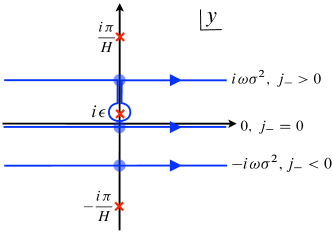
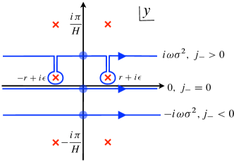
Figure 1: Contours of $y$ integration for $C_{j_{1}j_{2}}^{|\alpha_{1}-\alpha_{2}|}$. Cross symbols represent poles of $D_{\text{conf}}$ and disks represent saddle points of integrand. Left panel: $\alpha_{1}=\alpha_{2}~{}(r_{12}=0)$, Right panel : $\alpha_{1}\neq\alpha_{2}~{}(r_{12}=r\neq 0)$.

The result for $\alpha_{1}=\alpha_{2}~{}(r_{12}=0)$ is

$$C_{j_{1}j_{2}}^{0}=2\lambda^{2}e^{-\omega^{2}\sigma^{2}}\times\begin{cases}e^{i\omega\sigma j_{+}}\left(\sigma D_{2}(r_{12}=0,x=t+\sigma+\frac{i}{2}\omega\sigma^{2}j_{+},y=0)+\frac{1}{8\pi^{2}\sigma}\right)&\quad(C_{++}^{0},C_{--}^{0})\\ \sigma D_{\text{min}}(r_{12}=0,x=t+\sigma,y=i\omega\sigma^{2})+\frac{\omega e^{\omega^{2}\sigma^{2}}}{4\pi^{1/2}}&\quad(C_{+-}^{0})\\ \sigma D_{\text{min}}(r_{12}=0,x=t+\sigma,y=-i\omega\sigma^{2})&\quad(C_{-+}^{0})\end{cases}$$ (33)

where $1/(8\pi^{2}\sigma)$ and $\omega e^{\omega^{2}\sigma^{2}}/(4\pi^{1/2})$ are contributions from the pole $i\epsilon$ in $D_{\text{conf}}$.

For $\alpha_{1}\neq\alpha_{2}~{}(r_{12}=r\neq 0)$,

$$C_{j_{1}j_{2}}^{1}=2\lambda^{2}e^{-\omega^{2}\sigma^{2}}\times\begin{cases}e^{i\omega\sigma j_{+}}\sigma D_{\text{min}}(r,t+\sigma+\frac{i}{2}\omega\sigma^{2}j_{+},y=0)&\quad(C_{++}^{1},C_{--}^{1})\\ \sigma D_{\text{min}}(r,t+\sigma,i\omega\sigma^{2})+2i\pi^{1/2}\mathrm{Res}\left[e^{-(y-i\omega\sigma^{2})^{2}/\sigma^{2}}D_{\text{conf}}(r,t+\sigma,y)\right]&\quad(C_{+-}^{1})\\ \sigma D_{\text{min}}(r,t+\sigma,-i\omega\sigma^{2})&\quad(C_{-+}^{1})\end{cases}$$ (34)

where the residue (sum of contributions of two poles) is

$$\mathrm{Res}[\cdots]=\frac{1-\exp\left[\frac{4i\omega}{H}\sinh^{-1}\left(e^{H\sigma}Hr_{p}/2\right)\right]}{8\pi^{2}r_{p}(4+e^{2H\sigma}(Hr_{p})^{2})^{1/2}}\times\exp\left[-H\sigma+\left(\omega\sigma-\frac{i}{H\sigma}\sinh^{-1}(e^{H\sigma}Hr_{p}/2)\right)^{2}\right],\quad r_{p}=re^{Ht}.$$ (35)

II.2.2 Coefficients $H_{j_{1}j_{2}}^{|\alpha_{1}-\alpha_{2}|}$

The contours of integration is shown in Fig. 2.

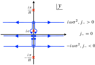
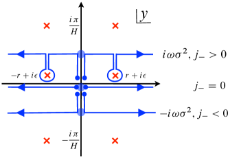
Figure 2: Contours of $y$ integration for $H_{j_{1}j_{2}}^{|\alpha_{1}-\alpha_{2}|}$. Left panel: $\alpha_{1}=\alpha_{2}~{}(r_{12}=0)$, Right panel: $\alpha_{1}\neq\alpha_{2}~{}(r_{12}=r\neq 0)$.

For $\alpha_{1}=\alpha_{2}$, contribution from saddles to the integrals cancels out and we only have contribution from a pole and contours along the imaginary $y$ axis:

$$H_{j_{1}j_{2}}^{0}=\begin{cases}\frac{1}{\epsilon}+I_{1}&\quad(H_{+-}^{0})\\ 0&\quad(H_{++}^{0},H_{--}^{0})\\ -I_{1}&\quad(H_{-+}^{0})\end{cases}$$ (36)

where $I_{1}$ is a finite contribution from contours along $\mathrm{Im}(y)$ axis and its explicit form is not necessary in the present analysis. The coefficients $H_{+-}^{0}$ diverges as $\epsilon\rightarrow 0$ and we will see this divergence can be renormalized to $\omega$ (Lamb shift). For $\alpha_{1}\neq\alpha_{2}~{}(r_{12}=r\neq 0)$,

$$H_{j_{1}j_{2}}^{1}=\begin{cases}4i\pi^{1/2}\lambda^{2}e^{-\omega^{2}\sigma^{2}}e^{i\omega\sigma j_{+}}\left(\mathrm{Res}_{1}-\mathrm{Res}_{2}\right)+I_{2}&\quad(H_{+-}^{1})\\ 0&\quad(H_{++}^{1},H_{--}^{1})\\ -I_{2}&\quad(H_{-+}^{1})\end{cases}$$ (37)

where $\mathrm{Res}_{1,2}$ denotes residues of two poles and $I_{2}$ is a contributions from contours along $\mathrm{Im}(y)$ axis, we do not need their explicit form here.

II.3 Components of master equation

We consider the density matrix with the following components

$$\rho=\begin{pmatrix}\rho_{11}&0&0&\rho_{14}\\ 0&\rho_{22}&\rho_{23}&0\\ 0&\rho_{23}^{*}&\rho_{33}&0\\ \rho_{14}^{*}&0&0&\rho_{44}\end{pmatrix},\quad\rho_{11}+\rho_{22}+\rho_{33}+\rho_{44}=1,$$ (38)

and we adopt the basis of the state $\{|11\rangle,|10\rangle,|01\rangle,|00\rangle\}$. We can check that this form of the density matrix is compatible with structure of the master equation and evolution keeps the structure of the matrix (38). By introducing new symbols for coefficients,

$$c^{0}_{11}=C_{++}^{0}=(C_{--}^{0})^{*},\quad c^{0}_{12}=C_{+-}^{0},\quad c^{0}_{21}=C_{-+}^{0},$$

$$c_{11}^{1}=C_{++}^{1}=(C_{--}^{1})^{*},\quad c_{12}^{1}=C_{+-}^{1},\quad c_{21}^{1}=C_{-+}^{1}.$$

The components of $\mathcal{L}[\rho]$ in the master equation (19) are

$$L_{11}=-2{c^{0}_{12}}\rho_{11}+{c^{0}_{21}}\rho_{22}+{c^{0}_{21}}\rho_{33}-{c_{11}^{1}{}^{*}}\rho_{14}-{c_{11}^{1}}\rho_{14}{}^{*}+{c_{21}^{1}}\rho_{23}+c_{21}^{1}\rho_{23}{}^{*},$$

$$L_{14}={c^{0}_{11}}\rho_{23}{}^{*}+{c^{0}_{11}}\rho_{23}-({c^{0}_{12}}+{c^{0}_{21}})\rho_{14}+{c_{11}^{1}}\left(-\rho_{11}-\rho_{44}+\rho_{22}+\rho_{33}\right),$$

$$L_{22}={c^{0}_{12}}\rho_{11}-({c^{0}_{12}}+{c^{0}_{21}})\rho_{22}+{c^{0}_{21}}\rho_{44}-\frac{1}{2}\left(c_{12}^{1}+c_{21}^{1}\right)\rho_{23}-\frac{1}{2}\left(c_{12}^{1}+c_{21}^{1}\right){\rho_{23}{}^{*}}+{c_{11}^{1}{}^{*}}\rho_{14}+{c_{11}^{1}}\rho_{14}{}^{*},$$

$$L_{23}=c_{12}^{1}\rho_{11}-\frac{1}{2}(c_{12}^{1}+c_{21}^{1})(\rho_{22}+\rho_{33})+c_{21}^{1}\rho_{44}+c^{0}_{11}{}^{*}\rho_{14}+{c_{11}^{1}}\rho_{14}{}^{*}-({c^{0}_{12}}+{c^{0}_{21}})\rho_{23},$$

$$L_{33}={c^{0}_{12}}\rho_{11}-({c^{0}_{12}}+{c^{0}_{21}})\rho_{33}+{c^{0}_{21}}\rho_{44}-\frac{1}{2}\left(c_{12}^{1}+c_{21}^{1}\right)\rho_{23}-\frac{1}{2}\left(c_{12}^{1}+c_{21}^{1}\right)\rho_{23}{}^{*}+{c_{11}^{1}{}^{*}}\rho_{14}+{c_{11}^{1}}\rho_{14}{}^{*},$$

$$L_{41}=-({c^{0}_{12}}+{c^{0}_{21}})\rho_{14}{}^{*}+c^{0}_{11}{}^{*}\rho_{23}{}^{*}+c^{0}_{11}{}^{*}\rho_{23}+{c_{11}^{1}{}^{*}}\left(-\rho_{11}-\rho_{44}+\rho_{22}+\rho_{33}\right),$$

$$L_{44}={c^{0}_{12}}\rho_{22}+{c^{0}_{12}}\rho_{33}-2{c^{0}_{21}}\rho_{44}-c_{11}^{1}{}^{*}\rho_{14}-{c_{11}^{1}}\rho_{14}{}^{*}+{c_{12}^{1}}\rho_{23}+{c_{12}^{1}}\rho_{23}{}^{*}.$$

The components of $i[H_{\text{eff}},\rho]$ in the master equation (19) are

$${\small\begin{pmatrix}0&0&0&2i\omega_{R}\rho_{14}\\ 0&(H_{+-}^{1}+H_{-+}^{1})(\rho_{23}^{*}-\rho_{23})/2&(H_{+-}^{1}+H_{-+}^{1})(\rho_{33}-\rho_{22})/2&0\\ 0&(H_{+-}^{1}+H_{-+}^{1})(\rho_{22}-\rho_{33})/2&(H_{+-}^{1}+H_{-+}^{1})(\rho_{23}-\rho_{23}^{*})/2&0\\ -2i\omega_{R}\rho_{14}^{*}&0&0&0\\ \end{pmatrix}}$$

where $\omega_{R}=\omega+(H^{0}_{+-}-H^{0}_{-+})/(2i)$ is a renromalized frequency. From now on, we denote $\omega_{R}$ as $\omega$. In our analysis, we consider the initial state $\rho_{0}=|00\rangle\langle 00|$. For this initial condition, $\rho_{22}=\rho_{33}$ and $\mathrm{Im}(\rho_{23})=0$ are kept during time evolution and we do not have to take into account of $H_{+-}^{1}+H_{-+}^{1}$ in the master equation.

As a measure of entanglement between two detectors, we adopt the negativity in our analysis. This quantity is introduced via partial transposition of the state of (38):

$$\rho^{PT}=\begin{pmatrix}\rho_{11}&0&0&\rho_{23}\\ 0&\rho_{22}&\rho_{14}&0\\ 0&\rho_{14}^{*}&\rho_{33}&0\\ \rho_{23}^{*}&0&0&\rho_{44}\end{pmatrix}.$$

The eigenvalues of this state are

$$\lambda=\frac{1}{2}\left[(\rho_{22}+\rho_{33})\pm\sqrt{(\rho_{22}-\rho_{33})^{2}+4\rho_{14}\rho_{14}^{*}}\right],\quad\frac{1}{2}\left[(\rho_{11}+\rho_{44})\pm\sqrt{(\rho_{11}-\rho_{44})^{2}+4\rho_{23}\rho_{23}^{*}}\right].$$

The definition of the negativity is

$$E_{N}\equiv\sum_{\lambda_{i}<0}|\lambda_{i}|,$$

and $E_{N}>0$ provides a necessary and sufficient condition for entanglement between two qubits Peres1996 ; Horodecki1996 . For the initial separable state $\rho_{0}=|00\rangle\langle 00|$, the solution of the master equation (19) around the initial time $t=0$ is

$$\rho(t)=\begin{pmatrix}0&0&0&-c_{11}^{1}t\\ 0&c^{0}_{21}t&c_{21}^{1}t&0\\ 0&c_{21}^{1}t&c^{0}_{21}t&0\\ -(c_{11}^{1})^{*}t&0&0&1-2c^{0}_{21}t\end{pmatrix}.$$

For this state, the negativity is given by

$$E_{N}=\max[0,t(|c_{11}^{1}|-c^{0}_{21})],\quad t\ll 1.$$ (39)

This formula is the same as one obtained by perturbation calculation Steeg2009 ; Nambu2011 ; Nambu2013 ; Martin-Martinez2014 and the value of negativity grows proportional to time. Initial separable state instantly becomes entangled if $|c_{11}^{1}|-c_{21}^{0}>0$ and detectors can catch entanglement of the quantum field. Using the explicit formula of the coefficients,

$$|c_{11}^{1}|-c^{0}_{21}=2\lambda^{2}\sigma^{2}e^{-\omega^{2}\sigma^{2}}\Bigl{(}\left|D[r,t+\sigma+i\omega\sigma^{2},0]\right|-D[0,t+\sigma,-i\omega\sigma^{2}]\Bigr{)}.$$ (40)

III Bell-CHSH inequality

We can test violation of the Bell-CHSH inequality in de Sitter space. For this purpose, we extend our previous analysis of the Bell-CHSH inequality for detectors system Nambu2011 . Let us consider the following Bell operator:

$$\mathcal{B}_{\text{CHSH}}=\boldsymbol{a}\cdot\boldsymbol{\sigma}\otimes(\boldsymbol{b}+\boldsymbol{b}^{\prime})\cdot\boldsymbol{\sigma}+\boldsymbol{a}^{\prime}\cdot\boldsymbol{\sigma}\otimes(\boldsymbol{b}-\boldsymbol{b}^{\prime})\cdot\boldsymbol{\sigma},$$ (41)

where $\boldsymbol{a},\boldsymbol{a}^{\prime},\boldsymbol{b},\boldsymbol{b}^{\prime}$ are real unit vectors. The Bell-CHSH inequality is

$$|\langle\mathcal{B}_{\text{CHSH}}\rangle|\leq 2.$$ (42)

If the state admits a local hidden variable (LHV) description of correlations, then this inequality holds. Violation of the inequality means existence of non-locality. We consider Bloch representation of the state (38):

$$\rho=\frac{1}{4}\left[I\otimes I+\boldsymbol{a}\cdot\boldsymbol{\sigma}\otimes I+I\otimes\boldsymbol{b}\cdot\boldsymbol{\sigma}+\sum_{j,k=1}^{3}c_{jk}\,\sigma_{j}\otimes\sigma_{k}\right],$$ (43)

$$\boldsymbol{a}=(0,0,\rho_{11}+\rho_{22}-\rho_{33}-\rho_{44}),\quad\boldsymbol{b}=(0,0,\rho_{11}+\rho_{33}-\rho_{22}-\rho_{44}),$$ (44)

$$c_{jk}=\begin{pmatrix}2\rho_{23}-2(\rho_{14})_{R}&2(\rho_{14})_{I}&0\\ 2(\rho_{14})_{I}&2\rho_{23}+2(\rho_{14})_{R}&0\\ 0&0&\rho_{11}+\rho_{44}-\rho_{22}-\rho_{33}\end{pmatrix}.$$ (45)

It is known this state violates the Bell-CHSH inequality if and only if the following condition is satisfied Horodecki1995a :

sum of the two largest eigenvalues of the matrix $$c\,c^{\dagger} >1$$  (46)

The eigenvalues of $c\,c^{\dagger}$ are

$$4(\rho_{11}+\rho_{44}-1/2)^{2},\quad 4(|\rho_{14}|\pm\rho_{23})^{2}.$$ (47)

For the initial separable state $\rho_{0}=|00\rangle\langle 00|$, we cannot expect these eigenvalues exceed unity after evolution because only non-zero component of the initial state is $\rho_{44}=1$. However, the Bell-CHSH inequality provides only a necessary condition for the LHV description and does not guarantee existence of a LHV Gisin1996a . Hence by passing each detector through the local filter

$$f_{A,B}=\begin{pmatrix}1&0\\ 0&\eta\end{pmatrix},$$ (48)

there is a possibility revealing hidden non-locality of the state. After passing through the filter, the state is transformed as $\rho^{\prime}=(f_{A}\otimes f_{B})\rho(f_{A}\otimes f_{B})$ and the normalized state is

$$\rho^{\prime}=\frac{1}{\rho_{11}+\eta^{2}(\rho_{22}+\rho_{33})+\eta^{4}\rho_{44}}\begin{pmatrix}\rho_{11}&0&0&\eta^{2}\rho_{14}\\ 0&\eta^{2}\rho_{22}&\eta^{2}\rho_{23}&0\\ 0&\eta^{2}\rho_{23}&\eta^{2}\rho_{33}&0\\ \eta^{2}\rho_{14}^{*}&0&0&\eta^{4}\rho_{44}\end{pmatrix}.$$ (49)

The matrix $c$ becomes

$$c^{\prime}=\frac{2\eta^{2}}{\rho_{11}+\eta^{2}(\rho_{22}+\rho_{33})+\eta^{4}\rho_{44}}\begin{pmatrix}\rho_{23}-(\rho_{14})_{R}&(\rho_{14})_{R}&0\\ (\rho_{14})_{R}&\rho_{23}+(\rho_{14})_{R}&0\\ 0&0&\frac{\rho_{11}-\eta^{2}(\rho_{22}+\rho_{33})+\eta^{4}\rho_{44}}{2\eta^{2}}\end{pmatrix}.$$ (50)

The eigenvalues of $c$ are

$$\frac{\rho_{11}-\eta^{2}(\rho_{22}+\rho_{33})+\eta^{4}\rho_{44}}{\rho_{11}+\eta^{2}(\rho_{22}+\rho_{33})+\eta^{4}\rho_{44}},\quad\frac{2\eta^{2}(\rho_{23}\pm|\rho_{14}|)}{\rho_{11}+\eta^{2}(\rho_{22}+\rho_{33})+\eta^{4}\rho_{44}},$$ (51)

and the condition for violation of the Bell-CHSH inequality is

$$0>\eta^{4}-\frac{(\rho_{23}+|\rho_{14}|)^{2}}{\rho_{44}(\rho_{22}+\rho_{33})}\eta^{2}+\frac{\rho_{11}}{\rho_{44}}.$$ (52)

The real parameter $\eta$ satisfying this inequality exists if the following condition holds

$$(\rho_{23}+|\rho_{14}|)^{4}>4\rho_{11}\rho_{44}(\rho_{22}+\rho_{33})^{2}.$$ (53)

This inequality provides a sufficient condition for violation of the Bell-CHSH inequality and if this inequality is satisfied, violation of the Bell-CHSH inequality can be detected.

IV Evolution of entanglement

We solve the master equation (19) numerically and follow evolution of entanglement between two detectors and test violation of the Bell-CHSH inequality. We used Mathematica and NDSolve to obtain numerical solutions.

IV.1 Minkowski vacuum

We first show parameters for initial detection of entanglement determined by Eq. (39) (Fig. 3). For any values of $r$, detection of entanglement is possible if we choose values of $\sigma$ above these lines.

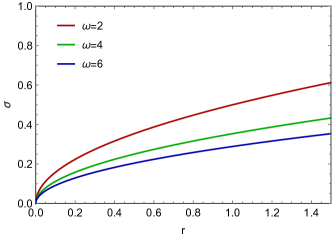
Figure 3: The negativity zero lines determined by (39). For parameters in regions above these lines, detectors can detect entanglement of the quantum field around initial time.

Our main interest is fate of detected entanglement after evolution. Fig. 4 contains density plots of the negativity in $(r,t)$ space and shows evolution of entanglement. The detector’s world line is $r=$constant in these figures. Although evolution of negativity is different for different $r$ and $\omega$, if the detectors do not catch the entanglement around $t\sim 0$, they cannot detect non-zero negativity even after evolution.

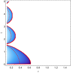
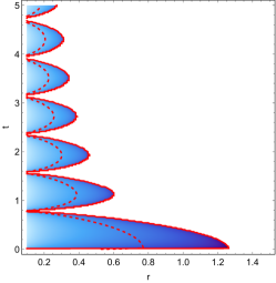
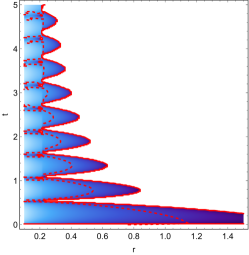
Figure 4: Evolution of negativity for $\omega=2,4,6$ with $\lambda=0.1,\sigma=0.4$. Detectors world lines are $r=$const. Detectors are entangled in regions enclosed by red solid lines (negativity zero lines). Violation of the Bell-CHSH inequality can be detected for parameters in regions enclosed by dotted lines.

As examples of evolution of negativity, we show its time dependence for $\omega=6,\sigma=0.4$ with two different $r$ (Fig. 5):

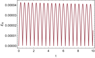
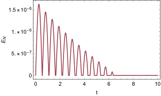
Figure 5: Time dependence of the negativity for $\lambda=0.1,\omega=6,\sigma=0.4$. Left: $r=0.05$. Right: $r=0.25$.

The negativity shows oscillatory behavior with a period $2\pi/\omega$. For both $r$, detectors can catch the entanglement of the field initially. For $r=0.05$, after initial detection of entanglement, the negativity decays linearly in time with oscillation. For $r=0.25$, the negativity decays also linearly in time, and after death and revival of entanglement several times, the negativity settles down to zero. Concerning the Bell-CHSH inequality, as shown in Fig. 4, violation of the inequality can be detectable for parameters in regions enclosed by dotted lines. These regions are contained in regions determined by zero negativity lines because non-zero values of the negativity provide a necessary condition for violation of the Bell-CHSH inequality.

For a larger value of the coupling constant $\lambda=0.5$, the negativity evolves as follows (Fig. 6, Fig. 7)

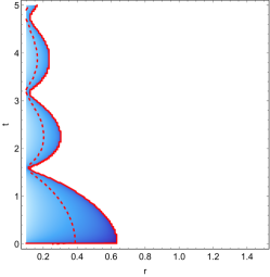
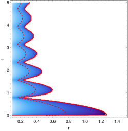
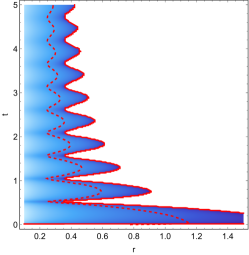
Figure 6: Evolution of negativity for $\omega=2,4,6$ with $\lambda=0.5,\sigma=0.4$. Detectors world lines are $r=$const. Detectors are entangled in regions enclosed by red solid lines (negativity zero lines). Violation of the Bell-CHSH inequality can be detected for parameters in regions enclosed by dotted lines.

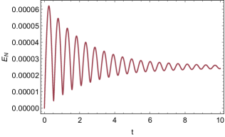
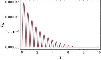
Figure 7: Time dependence of the negativity for $\lambda=0.5,\omega=6,\sigma=0.4$. Left: $r=0.2$. Right: $r=0.4$.

For $r=0.2$, after initial detection of entanglement, the negativity approaches a non-zero constant value. But for $r=0.4$, after death and revival of entanglement several times, the negativity settles down to zero and the state of the detectors finally becomes separable. From Fig. 6, we can observe that the detectors’ system approaches stationary state after elapsed time $\sim\sigma/\lambda^{2}$.

IV.2 Massless scalar field in de Sitter space

We consider the massless conformal scalar field and the massless minimal scalar field in de Sitter space.

IV.2.1 Conformal scalar

For the massless conformal scalar field, the negativity around initial time is determined by Eq. (39)

$$|c_{11}^{1}|-c^{0}_{21}=\frac{\lambda^{2}e^{-\omega^{2}\sigma^{2}}}{2\pi^{2}\sigma}(\sigma H)^{2}\left[\frac{e^{-2H\sigma}}{(Hr)^{2}}-\frac{1}{4\sin^{2}(H\omega\sigma^{2})}\right].$$ (54)

From this, we can estimate the maximum distance for entanglement detection (Fig. 8)

$$r\leq\frac{2}{H}\,e^{-\left(\frac{\pi H}{2\omega}\right)^{1/2}}<\frac{2}{H}.$$ (55)

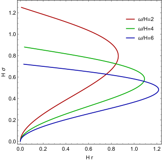
Figure 8: Parameters of entanglement detection around $t=0$. Entanglement can be detected for parameters in regions enclosed by each lines.

Thus, for large values of $\omega$, initial detection of entanglement beyond the Hubble horizon scale up to $2H^{-1}$ is possible for the conformal scalar field.

Evolution of the negativity is shown in Fig. 9. After initial detection of entanglement, the negativity finally becomes zero for large separation. For $\omega/H=2,4$, initial detection of entanglement is possible only for $r<H^{-1}$ and the detected entanglement survives beyond the super horizon scale $>H^{-1}$ if the separation of two detectors is small enough. For $\omega/H=6$, initial detection of entanglement for super horizon scale is possible (about $1.1H^{-1}$ in this case). Also in this case, for sufficiently small $r$, the detected entanglement survives when the physical separation of two detectors exceeds the Hubble horizon scale. Violation of Bell-CHSH inequality beyond the Hubble horizon scale detectable for sufficiently small $r$ (middle and right panels of Fig. 9).

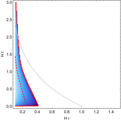
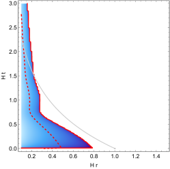
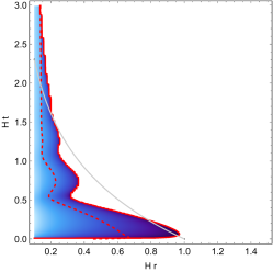
Figure 9: Evolution of negativity between comoving detectors for $\omega/H=2,4,6$ with $\lambda=0.1,\sigma H=0.4$. The detector’s world lines are $r=\text{const.}$ The gray solid lines represent comoving size of the Hubble horizon. The red solid lines represent negativity zero contours. Detectors are entangled for parameters in regions enclosed by the solid red lines. For parameters in regions enclosed by red dotted lines, violation of Bell’s inequality can be detected.

Fig. 10 shows time evolution of the negativity for $\omega/H=6$ with two different $r$. Behavior of evolution depends on $r$. For $rH=0.15$, the negativity remains non-zero after horizon exit. For $rH=0.3$, entanglement finally becomes zero.

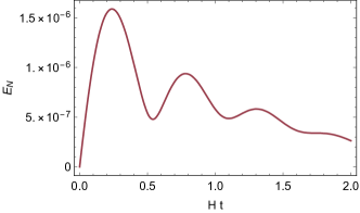
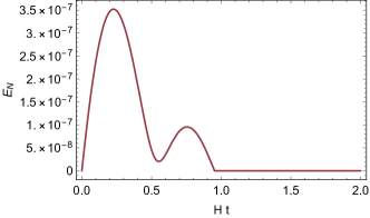
Figure 10: Evolution of negativity for $\lambda=0.1,\omega/H=6$ at $rH=0.15$ (left) and at $rH=0.3$ (right).

Evolution of negativity for $\lambda=0.5$ is shown in Fig. 11 and Fig. 12. Also in this case, detected entanglement can survive beyond the Hubble horizon scale for small $r$.

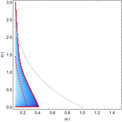
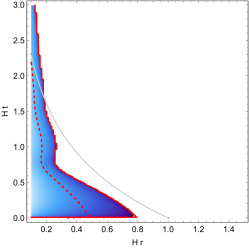
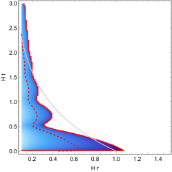
Figure 11: Evolution of negativity between comoving detectors for $\omega/H=2,4,6$ with $\lambda=0.5,\sigma H=0.4$. The detector’s world lines are $r=\text{const.}$ The gray solid lines represent comoving size of the Hubble horizon. The red solid lines represent negativity zero contours. Detectors are entangled for parameters in regions enclosed by the solid red lines. For parameters in regions enclosed by red dotted lines, violation of Bell’s inequality can be detected.

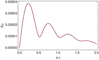
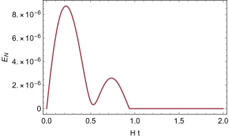
Figure 12: Evolution of negativity for $\lambda=0.5,\omega/H=6$ at $rH=0.15$ (left) and at $rH=0.3$ (right).

IV.2.2 Massless minimal scalar

Initial detection of entanglement determined by Eq. (39) (Fig. 13) . Compared to the conformal scalar case, the maximum distance of the entanglement detection is reduced and detection is possible only for $r<0.6H^{-1}$ (sub horizon scale).

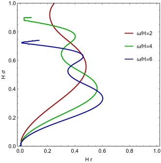
Figure 13: Parameters of initial detection of entanglement. Entanglement of the minimal scalar field can be detected for parameters in the regions enclosed by each lines.

Evolution of negativity is shown in Fig. 14 and Fig. 15. The behavior is almost same as that of the conformal scalar field apart from initial spatial scale of entanglement detection. As a result of evolution, for any values of $r$, detected entanglement of the scalar field vanishes before separation between two detectors exceeds the Hubble horizon scale. This behavior is contrasted with the result of the conformal scalar field, in which case the entanglement can extend beyond the Hubble horizon for sufficiently small $r$. For the minimal scalar field, particle creations in de Sitter space works as a noise and destroys the quantum coherence over the Hubble scale. As a result, the detectors can not catch the entanglement of the quantum field for the scale larger than the Hubble horizon.

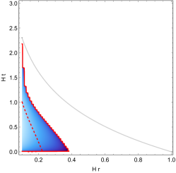
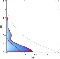
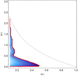
Figure 14: Evolution of negativity for between comoving detectors $\omega/H=2,4,6$ with $\lambda=0.1,\sigma H=0.4$. Detectors’ world lines are $r=\text{const.}$ The gray solid line represents comoving size of the Hubble horizon and the red solid lines represent negativity zero contours. Detectors are entangled for parameters in regions enclosed by the solid red lines. For parameters in regions enclosed by the red dotted line, violation of Bell’s inequality can be detected.

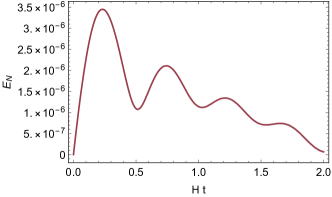
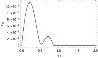
Figure 15: Evolution of negativity for $\lambda=0.1,\omega/H=6$ at $rH=0.1$ (left) and at $rH=0.2$ (right).

Fig. 16 and Fig. 17 show evolution of negativity for $\lambda=0.5$.

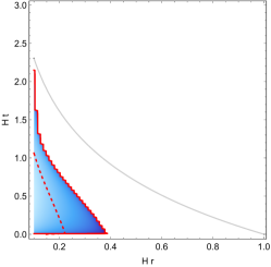
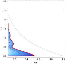
Figure 16: Evolution of negativity for between comoving detectors $\omega/H=2,4,6$ with $\lambda=0.5,\sigma H=0.4$. Detectors’ world lines are $r=\text{const.}$ The gray solid line represents comoving size of the Hubble horizon and the red solid lines represent negativity zero contours. Detectors are entangled for parameters in regions enclosed by the solid red lines. For parameters in regions enclosed by the red dotted line, violation of Bell’s inequality can be detected.

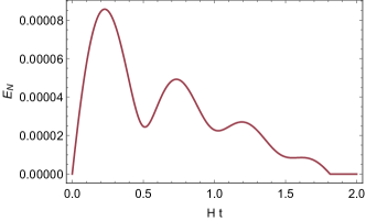
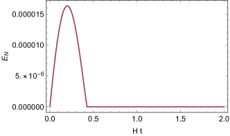
Figure 17: Evolution of negativity for $\lambda=0.5,\omega/H=6$ at $rH=0.1$ (left) and at $rH=0.2$ (right).

V Summary

We investigated evolution of entanglement between two detectors in de Sitter space. We adopt the master equation with DCG approximation to obtain evolution of the negativity between two detectors interacting with the quantum scalar field. For the massless conformal scalar field with the conformal vacuum, after evolution, two detectors can catch the entanglement of the scalar field beyond the horizon scale if the initial comoving separation is sufficiently small. At the same time, violation of the Bell-CHSH inequality is detectable for scales larger than the Hubble horizon. This behavior cannot be obtained previous analysis based on naive perturbation Nambu2011 ; Nambu2013 . On the other hand, for the massless minimal scalar field with the Bunch-Davies vacuum, the detected negativity decays within a Hubble time scale and two detectors become separable before their physical distance exceeds the Hubble horizon. This behavior is consistent with the result obtained by considering bipartite entanglement between two spatial regions introduced by averaging Nambu2008 ; Nambu2009 . Thus the result obtained in this paper supports appearance of classical nature of fluctuations in the inflationary universe.

We should comment on relation to our recent lattice simulation of negativity in de Sitter space Matsumura2017 . We discretize the minimal scalar field in de Sitter space and evaluated negativity between two spatial regions in the 1-dim lattice. The analysis shows that the entanglement on the super horizon scale always remains. This result must be contrasted with the result obtained by the master equation in this paper, which shows detectors cannot catch entanglement beyond the Hubble horizon scale. At this stage, we can only say that detection of entanglement using a pair of two detectors (bipartite entanglement in the present case) is not so effective and there may be a possibility that the super horizon scale entanglement can be detectable by considering effect of the multi-partite entanglement. We will report on this subject in our next publication Kukita2017b .

- (1) M. A. Nielsen and I. L. Chuang, Quantum computation and Quantum Information (Cambridge University Press, 2000).
- (2) Y. Nambu, “Entanglement of quantum fluctuations in the inflationary universe”, Phys. Rev. D 78, (2008) 044023.
- (3) Y. Nambu and Y. Ohsumi, “Entanglement of a coarse grained quantum field in the expanding universe”, Phys. Rev. D 80, (2009) 124031.
- (4) Y. Nambu and Y. Ohsumi, “Classical and quantum correlations of scalar field in the inflationary universe”, Phys. Rev. D 84, (2011) 044028.
- (5) Y. Nambu, “Entanglement Structure in Expanding Universes”, Entropy 15, (2013) 1847–1874.
- (6) W. G. Unruh, “Notes on black-hole evaporation”, Phys. Rev. D 14, (1976) 870–892.
- (7) B. S. DeWitt, “Quantum gravity: the new synthesis”, in “General relataivity An Einstein Centenary Survey”, 680–745 (Cambridge University Press, 1979).
- (8) N. D. Birrell and P. C. W. Davies, Quantum fields in curved space (Cambridge University Press, 1984).
- (9) G. V. Steeg and N. C. Menicucci, “Entangling power of an expanding universe”, Phys. Rev. D 79, (2009) 044027.
- (10) E. Martin-Martinez and N. C. Menicucci, “Entanglement in curved spacetimes and cosmology”, Class. Quantum Gravity 31, (2014) 214001.
- (11) H. P. Breuer and F. Petruccione, The Theory of Open Quantum Systems (Oxford, 2002).
- (12) V. Gorini, A. Kossakowski, and E. C. G. Sudarshan, “Completely positive dynamical semigroups of N-level systems”, J. Math. Phys. 17, (1976) 821.
- (13) G. Lindblad, “On the generators of quantum dynamical semigroups”, Commun. Math. Phys. 48, (1976) 119–130.
- (14) H. Yu and J. Zhang, “Understanding Hawking radiation in the framework of open quantum systems”, Phys. Rev. D 77, (2008) 024031.
- (15) J. Hu and H. Yu, “Quantum entanglement generation in de Sitter spacetime”, Phys. Rev. D 88, (2013) 104003.
- (16) Z. Tian and J. Jing, “Dynamics and quantum entanglement of two-level atoms in de Sitter spacetime”, Ann. Phys. (N. Y). 350, (2014) 1–13.
- (17) J. Hu and H. Yu, “Entanglement dynamics for uniformly accelerated two-level atoms”, Phys. Rev. A 91, (2015) 012327.
- (18) Z. Tian, J. Wang, J. Jing, and A. Dragan, “Detecting the Curvature of de Sitter Universe with Two Entangled Atoms”, Scientific Reports 6, (2016) 35222.
- (19) D. A. Lidar, Z. Bihary, and K. Whaley, “From completely positive maps to the quantum Markovian semigroup master equation”, Chem. Phys. 268, (2001) 35–53.
- (20) G. Schaller and T. Brandes, “Preservation of positivity by dynamical coarse graining”, Phys. Rev. A 78, (2008) 022106.
- (21) F. Benatti, R. Floreanini, and U. Marzolino, “Entangling two unequal atoms through a common bath”, Phys. Rev. A 81, (2010) 012105.
- (22) C. Majenz, T. Albash, H.-P. Breuer, and D. a. Lidar, “Coarse graining can beat the rotating-wave approximation in quantum Markovian master equations”, Phys. Rev. A 88, (2013) 012103.
- (23) Y. Nambu and S. Kukita, “Derivation of Markovian Master Equation by Renormalization Group Method”, J. Phys. Soc. Japan 85, (2016) 114002.
- (24) A. Peres, “Separability Criterion for Density Matrices”, Phys. Rev. Lett. 77, (1996) 1413–1415.
- (25) M. Horodecki, P. Horodecki, and R. Horodecki, “Separability of mixed states: necessary and sufficient conditions”, Phys. Lett. A 223, (1996) 1–8.
- (26) R. Horodecki, P. Horodecki, and M. Horodecki, “Violating Bell’s inequality by mixed spin-1/2 states: necessary and sufficient condition”, Phys. Lett. A 200, (1995) 340–344.
- (27) N. Gisin, “Hidden quantum nonlocality revealed by local filters”, Phys. Lett. A 210, (1996) 151–156.
- (28) A. Matsumura and Y. Nambu, “Large scale Quantum entanglement in de Sitter spacetime”, arXiv:1707.08414 (2017).
- (29) S. Kukita and Y. Nambu, “Harvesting large scale entanglement in de Sitter space with multiple detectors”, Entropy 19, (2017) 449.