A fourth order gauge-invariant gradient plasticity model for polycrystals based on Kröner’s incompatibility tensor

Abstract

In this paper we derive a novel fourth order gauge-invariant phenomenological model of infinitesimal rate-independent gradient plasticity with isotropic hardening and Kröner’s incompatibility tensor $\operatorname{inc}(\mbox{$\bf\varepsilon$}_{p}):=\operatorname{Curl\hskip 1.13791pt}[(\operatorname{Curl\hskip 1.13791pt}\mbox{$\bf\varepsilon$}_{p})^{T}]$, where $\mbox{$\bf\varepsilon$}_{p}$ is the symmetric plastic strain tensor. Here, gauge-invariance denotes invariance under diffeomorphic reparametrizations of the reference configuration, suitably adapted to the geometrically linear setting. The model features a defect energy contribution which is quadratic in the tensor $\operatorname{inc}(\mbox{$\bf\varepsilon$}_{p})$ and it contains isotropic hardening based on the rate of the plastic strain tensor $\dot{\mbox{$\bf\varepsilon$}}_{p}$. We motivate the new model by introducing a novel rotational invariance requirement in gradient plasticity, which we call micro-randomness, suitable for the description of polycrystalline aggregates on a mesoscopic scale and not coinciding with classical isotropy requirements. This new condition effectively reduces the increments of the non-symmetric plastic distortion $\dot{p}$ to their symmetric counterpart $\dot{\mbox{$\bf\varepsilon$}}_{p}=\operatorname{sym}\dot{p}$. In the polycrystalline case, this condition is a statement about insensitivity to arbitrary superposed grain rotations. We formulate a mathematical existence result for a suitably regularized non-gauge-invariant model. The regularized model is rather invariant under reparametrizations of the reference configuration including infinitesimal conformal mappings.

Key words: plasticity, gradient plasticity, geometrically necessary dislocations, incompatible distortions, rate-independent models, kinematic hardening, backstress, Bauschinger effects, variational inequality, defect energy, incompatibility tensor, Riemann-Christoffel tensor, dislocation density, gauge theory of dislocations, Lanczos scalar, infinitesimal conformal mappings, isotropy. AMS 2010 subject classification: 35D30, 35D35, 74C05, 74C15, 74D10, 35J25.

1.  Introduction

In recent years there has been a growing attention in extending continuum plasticity theories towards the incorporation of the experimentally observed size-effects in small scales (see e.g. [47, 49, 118, 128]). This extension is mainly done via the introduction of certain gradient terms, making the plastic evolution in some sense nonlocal. Perhaps the earliest such phenomenological model is due to Aifantis et al. [3, 4, 93, 137], who directly incorporated the Laplacian $\Delta\gamma_{p}$ in the flow stress, where $\gamma_{p}:=\int_{0}^{t}\left\lVert{\dot{\mbox{$\bf\varepsilon$}}_{p}}\right\rVert\,ds$ is a measure of accumulated equivalent plastic strain (see Table 1 below for a summary).

$\operatorname{sym}\nabla u=\varepsilon=\varepsilon_{e}+\varepsilon_{p}$ , $\varepsilon_{p}\in\mbox{Sym}\,(3)$
$\sigma_{\mathrm{y}}=\sigma_{0}+\mu\,k_{2}\,\gamma_{p}-\mu\,L_{c}^{2}\,\Delta\gamma_{p}$ ,    $\sigma_{\mathrm{y}}$ is the current yield stress
$L_{c}>0$ material length scale
$\sigma_{0}>0$   the initial yield stress
$k_{2}$   can be taken negative for local softening behaviour
$\gamma_{p}:=\int_{0}^{t}\left\lVert{\dot{\varepsilon}_{p}}\right\rVert\,ds$   the accumulated equivalent plastic strain .

Table 1: A summary of the model by Aifantis [3, 4, 93] based on the accumulated equivalent plastic strain $\gamma_{p}$. Depending on the sign of $\Delta\gamma_{p}$, the model describes process-dependent hardening ($\Delta\gamma_{p}<0$) or softening ($\Delta\gamma_{p}>0$) due to nonlocal effects.

Other variants of the Aifantis’ model also based on the accumulated plastic strain were proposed later through the principle of virtual power by Fleck and Hutchinson [48], Gudmundson [53] and generalized by Gurtin and Anand [59].

While there are numerous proposals of such gradient enhanced phenomenological models, either based on the multiplicative decomposition

$$F=F_{e}\cdot F_{p}$$ (1.1)

(see e.g. [2, 28, 58, 101]), or based on the geometrically linearized corresponding additive decomposition

$$\mbox{$\bf\varepsilon$}=\mbox{$\bf\varepsilon$}_{e}+\mbox{$\bf\varepsilon$}_{p}$$ (1.2)

(see e.g. [3, 4, 93, 48, 53, 57, 59, 61, 85, 86, 93, 130]), no general consensus has been reached as to which variables describing the plastic evolution should be employed and how they should be combined with their partial derivatives in space. For example, a dependence of the plastic flow rule directly via the infinitesimal plastic strain variable $\mbox{$\bf\varepsilon$}_{p}$ is sometimes excluded, since the backstress variable $\mbox{$\bf\varepsilon$}_{p}$ is not gauge-invariant.

However, if $\mbox{$\bf\varepsilon$}_{p}$ is not allowed to appear itself in the equations, then linear kinematic hardening á la Prager is excluded from the onset, while the modelling of classical linear isotropic hardening remains possible since it is based on $\left\lVert{\dot{\mbox{$\bf\varepsilon$}}_{p}}\right\rVert$, which is invariant under reparametrization of the reference configuration (gauge-invariance), see subsection 3.1 in this paper.

With the use of an evolution equation for the symmetric plastic strain tensor $\mbox{$\bf\varepsilon$}_{p}$ being traditional, there are also approaches which focus directly on the plastic distortion $p$ (which is a non-symmetric variable), thus allowing for the so-called plastic spin (see [60, p.493 and eqs. (91.7) and (91.10)] and also [32, 69, 83, 15, 120, 17]). The connection between the two approaches is simple: we can always identify $\mbox{$\bf\varepsilon$}_{p}:=\operatorname{sym}p$. As it will turn out subsequently, the introduction of the plastic distortion $p$ will make our modelling framework much more transparent: on the one hand, the passage from the multiplicative decomposition to the additive decomposition via formal geometric linearization is easier and the discussion of invariance conditions becomes clearer, even if in the end we obtain a model for the plastic strain tensor $\mbox{$\bf\varepsilon$}_{p}=\operatorname{sym}p$ only.

Our aim with this paper is to present a rational modelling environment for gradient plasticity with respect to the small strain framework and the additive decomposition which incorporates certain insights learned from the multiplicative decomposition.

Let us therefore collect what the model should be able to do. It should

• incorporate energetic hardening (due to Geometrically Necessary Dislocations, GNDs) related to the energetic length scale $L_{c}$;

• incorporate nonlocal hardening (backstress and Bauschinger effects);

• satisfy appropriate invariance conditions (objectivity, referential isotropy, independence of reference configuration, gauge-invariance, elastic isotropy, elastic frame-indifference, etc.);

• allow in principle for plastic spin (Bardella [15, 16], Gurtin [56], Neff et al. [101], Ebobisse et al. [38, 42, 41]);

• satisfy an extended positive dissipation principle and be therefore thermodynamically admissible;

• be able to be cast in a convex analytical framework;

• support a well-posedness result in both the rate-independent and the rate-dependent cases;

• have physical meaningful and transparent boundary conditions for the plastic variables.

In this paper, we will propose such a model, which, in the end, has a certain resemblance with the early model proposed by Menzel and Steinmann [86] and we will show its well-posedness in the rate-independent case with a suitable regularization. Our derivation of the model based on invariance principles is, to our knowledge, entirely new. The model is derived through a process of linearization of some state variables in the finite strain case. The derivation of a linear model from a finite strain one is not new in the context of elasto-plasticity. For instance, Mielke and Stefanelli [90] used $\Gamma$-convergence to derive rigorously a model of linearized plasticity as limit of some finite strain plasticity model.

The mathematical well-posedness of our model seems to be interesting in its own right. Once more, the convex analytical framework, based on incorporating the postulate of maximum plastic dissipation, put forward initially by Moreau [92] and used later by many authors (e.g. [62, 35, 123, 101, 37, 38, 39, 40, 42, 41]), proves to be ideally suited. For that purpose, our ”additive” model also admits a finite strain parent model by Krishnan and Steigmann [71], who did not consider, however, the incorporation of (nonlocal) kinematic hardening.

Decisive for our new strain gradient plasticity model is the introduction of Kröner’s incompatibility tensor $\operatorname{inc}$ ([72, 73, 67, 134, 135, 136]) as an inhomogeneity measure acting on the symmetric plastic strain $\mbox{$\bf\varepsilon$}_{p}=\operatorname{sym}p$. This incompatibility tensor is given by

$$\operatorname{inc}(\operatorname{sym}p):=\operatorname{Curl\hskip 1.13791pt}([\operatorname{Curl\hskip 1.13791pt}\operatorname{sym}p]^{T})\,$$ (1.3)

and it coincides to first order with the Riemann-Christoffel curvature tensor $\mathcal{R}$ in the metric characterized by the finite plastic strain tensor $C_{p}:={F_{p}\hskip-2.84544pt}^{T}\,\hskip-2.84544ptF_{p}$ (De Wit [34]). In fact, considering the non-symmetric plastic distortion $F_{p}$ in the multiplicative decomposition (1.1) and writing $F_{p}={\boldsymbol{\mathbbm{1}}}+p$, the connection is

$$\mathcal{R}({F_{p}\hskip-2.84544pt}^{T}\,\hskip-2.84544ptF_{p})=\mathcal{R}(({\boldsymbol{\mathbbm{1}}}+p)^{T}({\boldsymbol{\mathbbm{1}}}+p))=\mathcal{R}({\boldsymbol{\mathbbm{1}}}+2\operatorname{sym}p+p^{T}p)=2\operatorname{inc}(\operatorname{sym}p)+\mbox{h.o.t.},$$ (1.4)

where

$$\mathcal{R}^{i}_{jkl}(C_{p}):=\frac{\partial\Gamma^{i}_{jl}}{\partial x_{k}}-\frac{\partial\Gamma^{i}_{jk}}{\partial x_{l}}+\Gamma^{m}_{jl}\,\Gamma^{i}_{mk}-\Gamma^{m}_{jk}\,\Gamma^{i}_{ml}\,,$$ (1.5)

with

$$\Gamma^{l}_{ij}:=\frac{1}{2}g^{kl}\left[\frac{\partial g_{ki}}{\partial x_{j}}+\frac{\partial g_{jk}}{\partial x_{i}}-\frac{\partial g_{ij}}{\partial x_{k}}\right]$$

being the Christoffel symbols of the second kind in the metric $C_{p}=(g_{ij})$ whose inverse is $C_{p}^{-1}=(g^{ij})$. Assume that we change the reference configuration by a smooth invertible map

$$\psi:\xi\mapsto x(\xi)\,,$$ (1.6)

then the plastic distortion $F_{p}$ in the multiplicative decomposition (1.1) should transform according to

$$F_{p}(x)\,\longrightarrow\,F_{p}(x(\xi))\,\frac{\partial x(\xi)}{\partial\xi}=\widetilde{F}_{p}(\xi)\,\nabla_{\xi}\psi(\xi)\,.$$ (1.7)

Based on the Riemann-Christoffel curvature tensor $\mathcal{R}$ in (1.5), we may form a ”true scalar” quantity, namely the so-called Lanczos scalar

$$\sum_{ijkl}\mathcal{R}^{i}_{jkl}\cdot\mathcal{R}^{i}_{jkl}=:\left\lVert{\mathcal{R}}\right\rVert^{2}_{\mathbb{R}^{81}}\,,$$ (1.8)

which is form-invariant under a change of the reference configuration in the sense that

$$\left\lVert{\mathcal{R}_{x}({F_{p}(x)}^{T}\hskip-2.84544ptF_{p}(x))}\right\rVert^{2}=\left\lVert{\mathcal{R}_{\xi}((\widetilde{F}_{p}(\xi)\,\nabla_{\xi}\psi(\xi))^{T}(\widetilde{F}_{p}(\xi)\,\nabla_{\xi}\psi(\xi)))}\right\rVert^{2}\,,$$ (1.9)

(see Lanczos [75, eq. (2.3)]) where $\mathcal{R}_{x}$ and $\mathcal{R}_{\xi}$ denote the Riemann-Christoffel curvature tensor expressed in coordinates $x$ and $\xi$, respectively. Moreover, if we consider the transformation

$$F_{p}(x)\,\longrightarrow\,\widehat{F}_{p}:=Q(x)F_{p}(x),\quad\mbox{with arbitrary }Q(x)\in\operatorname{O}(3)\,,$$ (1.10)

then we have the direct invariance condition for the Riemann-Christoffel curvature tensor

$$\mathcal{R}_{x}({F_{p}(x)}^{T}\hskip-2.84544ptF_{p}(x)) = \mathcal{R}_{x}({F_{p}(x)}^{T}\hskip-2.84544ptQ(x)^{T}Q(x)F_{p}(x))=\mathcal{R}_{x}((Q(x)F_{p}(x))^{T}\hskip-2.84544ptQ(x)F_{p}(x))$$ (1.11)

$$= \mathcal{R}_{x}({\widehat{F}_{p}(x)}^{T}\hskip-2.84544pt\widehat{F}_{p}(x))\,.$$

The form-invariance property (1.9) is inherited in its geometric linearization, now by the $\operatorname{inc}$-operator, in the form of a direct invariance condition for the complete operator (and not just the “Lanczos”-type scalar $\left\lVert{\operatorname{inc}_{x}\operatorname{sym}p}\right\rVert^{2}$):

$$\operatorname{inc}_{x}(\operatorname{sym}p(x))=\operatorname{inc}_{x}(\operatorname{sym}(p(x)+\nabla_{x}\vartheta(x))\qquad\forall\,\vartheta(x)\in C^{\infty}(\mathbb{R}^{3},\,\mathbb{R}^{3})\,,$$ (1.12)

where we have identified $\psi(x)=x+\vartheta(x)$. In fact, from the identity (see [50, Proposition 2.1])

$$\nabla\operatorname{axl}(\mathop{\rm skew}\nabla\vartheta)=\frac{1}{2}\nabla\operatorname{curl\,}\vartheta=(\operatorname{Curl\hskip 1.13791pt}\operatorname{sym}\nabla\vartheta)^{T},$$ (1.13)

taking the Curl on both sides, we get

$$0=\operatorname{Curl\hskip 1.13791pt}\bigl{(}\frac{1}{2}\nabla\operatorname{curl\,}\vartheta\bigr{)}=\operatorname{Curl\hskip 1.13791pt}\bigl{[}(\operatorname{Curl\hskip 1.13791pt}\operatorname{sym}\nabla\vartheta)^{T}\bigr{]}=\operatorname{inc}(\operatorname{sym}\nabla\vartheta)\,,$$ (1.14)

which shows (1.12). Of course (1.12) implies that

$$\left\lVert{\operatorname{inc}_{x}(\operatorname{sym}p(x))}\right\rVert^{2}=\left\lVert{\operatorname{inc}_{x}(\operatorname{sym}(p(x)+\nabla_{x}\vartheta(x))}\right\rVert^{2}\qquad\forall\,\vartheta(x)\in C^{\infty}(\mathbb{R}^{3},\,\mathbb{R}^{3})\,,$$ (1.15)

mirroring property (1.9) for the Lanczos-type scalar. In addition, the direct invariance condition (1.11) for $\mathcal{R}$ under rotation fields $Q(x)\in\operatorname{SO}(3)$ translates to an invariance condition on the inc-operator as well. We write $Q(x)={\boldsymbol{\mathbbm{1}}}+A(x)+\mbox{h.o.t.}$ with $A(x)\in\operatorname{\mathfrak{so}}(3)$ and in terms of the infinitesimal plastic distortion, we consider

$$p(x)\,\longrightarrow\,A(x)+p(x)\qquad\forall A(x)\in\operatorname{\mathfrak{so}}(3)$$

and we have the invariance condition

$$\operatorname{inc}_{x}(\operatorname{sym}p(x))=\operatorname{inc}_{x}(\operatorname{sym}(A(x)+p(x)))\qquad\forall\,A(x)\in\operatorname{\mathfrak{so}}(3)\,.$$ (1.16)

For both tensors $\mathcal{R}$ and $\operatorname{inc}$ we note the Saint-Venant compatibility condition and its linearization:

$$\psi(x)=x+\vartheta(x) C_{p}=F_{p}^{T}\hskip-2.84544pt\,F_{p}={\boldsymbol{\mathbbm{1}}}+\mbox{$\bf\varepsilon$}_{p}+\mbox{h.o.t}$$     and    

(1.17)

$$C_{p}=F_{p}^{T}\hskip-2.84544pt\,F_{p}\in\mbox{Sym}^{+}(3) \mathcal{R}(C_{p})=0\,\Leftrightarrow\,C_{p}={\nabla\psi}^{T}\nabla\psi \approx \operatorname{inc}(\operatorname{sym}p)=0\,\Leftrightarrow\,\operatorname{sym}p=\operatorname{sym}\nabla\vartheta$$ symmetric positive definite See e.g. Ciarlet-Laurent [31, Theorem 1.1]

in simply connected domains (see [84, 30, 31, 80]). For more properties of the $\operatorname{inc}$-operator, we refer the reader to [134, 10, 80]. With these preliminaries, both tensors $\mathcal{R}$ and $\operatorname{inc}$ qualify as incompatibility measures on positive definite symmetric plastic strains $C_{p}=F_{p}^{T}\hskip-2.84544pt\,F_{p}$ in the geometrically nonlinear and on symmetric plastic strains $\mbox{$\bf\varepsilon$}_{p}=\operatorname{sym}p$ in the geometrically linear settings, respectively. In a purely phenomenological context, we have another way to measure the incompatibility of the plastic distortion $F_{p}$ itself via the so-called dislocation density tensor $\operatorname{Curl\hskip 1.13791pt}_{x}F_{p}(x)$ (see for instance [58, 101]). Following the works of Davini-Parry [33], Cermelli-Gurtin [28] and Epstein [44], it has been shown that the differential operator (the ”true dislocation density tensor”) 

$$\frac{1}{\det F_{p}}\,(\operatorname{Curl\hskip 1.13791pt}F_{p})\,F^{T}_{p}=\det F_{e}(\operatorname{Curl\hskip 1.13791pt}_{C}F_{e}^{-1})F_{e}^{-T}\,,$$ (1.18)

(where $\operatorname{Curl\hskip 1.13791pt}_{C}$ means taking the spatial Curl w.r.t. the current configuration) is also form-invariant under arbitrary coordinate transformation of the reference placement (see [28, eq.(1.4) on p.1542]). This property is easily understood from (1.18)₂, which is invariant under reparametrization of the reference system anyway.

From now on, we assume plastic incompressibility, i.e., $\det F_{p}=1$ and $\operatorname{tr}p=0$. Either

$$(\operatorname{Curl\hskip 1.13791pt}_{x}F_{p})\,F^{T}_{p}\quad\mbox{linearized through}\quad F_{p}={\boldsymbol{\mathbbm{1}}}+p\quad\mbox{turns into}\quad\operatorname{Curl\hskip 1.13791pt}_{x}p$$ (1.19)

or

$$\mathcal{R}({F_{p}\hskip-2.84544pt}^{T}\hskip-2.84544ptF_{p})\quad\mbox{linearized through}\quad F_{p}={\boldsymbol{\mathbbm{1}}}+p\quad\mbox{turns into}\quad\operatorname{inc}(\operatorname{sym}p)\,.$$ (1.20)

Therefore, in the geometrically linear setting two measures of incompatibility of the infinitesimal plastic distortion $p$ are used in the literature. Some authors use the tensor $\operatorname{Curl\hskip 1.13791pt}p$ (see [23, 24, 57, 101]) while others use $\operatorname{inc}(\operatorname{sym}p)$ (see [86]).

$\begin{array}[]{lcl}\operatorname{Curl\hskip 1.13791pt}p=0&\Rightarrow&p=\nabla\vartheta\\ &\Rightarrow&\operatorname{inc}(\operatorname{sym}p)=\operatorname{inc}(\operatorname{sym}\nabla\vartheta)=0\end{array}$

$\begin{array}[]{lcl}\operatorname{inc}(\operatorname{sym}p)=0&\Rightarrow&\operatorname{sym}p=\operatorname{sym}\nabla\vartheta\\ &/\hskip-9.95863pt\Rightarrow&p=\nabla\vartheta\,\,\mbox{ but}\\ &\Rightarrow&p=\nabla\vartheta+A(x),\quad A(x)\in\operatorname{\mathfrak{so}}(3)\\ &/\hskip-9.95863pt\Rightarrow&\operatorname{Curl\hskip 1.13791pt}p=0\end{array}$

Table 2: We need to realize that $\operatorname{Curl\hskip 1.13791pt}p$ is a “sharper” incompatibility measure than $\operatorname{inc}(\operatorname{sym}p)$.

Concerning the invariance of the curvature tensor $\mathcal{R}$ observed in (1.9), we note that under a change of reference placement $F_{p}(x)\,\longrightarrow\,\widetilde{F}_{p}(\xi)\,\nabla\psi(\xi)$, we obtain directly the form-invariance of the true dislocation density tensor $(\operatorname{Curl\hskip 1.13791pt}F_{p})\,F^{T}_{p}$ as well, meaning that

$$(\operatorname{Curl\hskip 1.13791pt}_{x}F_{p})\,F^{T}_{p}=(\operatorname{Curl\hskip 1.13791pt}_{\xi}(\widetilde{F}_{p}(\xi)\,\nabla\psi(\xi)))\,(\widetilde{F}_{p}(\xi)\,\nabla\psi(\xi))^{T}\,,$$ (1.21)

where $\operatorname{Curl\hskip 1.13791pt}_{x}$ and $\operatorname{Curl\hskip 1.13791pt}_{\xi}$ are the Curl expressed in coordinates $x$ and $\xi$, respectively. Therefore, the expression $\left\lVert{(\operatorname{Curl\hskip 1.13791pt}_{x}F_{p})\,F^{T}_{p}}\right\rVert^{2}$ is also a true scalar quantity. Accordingly, in the linearized setting we consider as in (1.12)

$$p(x)\,\longrightarrow\,p(x)+\nabla\vartheta(x)$$ (1.22)

and we obtain directly the invariance

$$\operatorname{Curl\hskip 1.13791pt}p(x)=\operatorname{Curl\hskip 1.13791pt}\bigl{[}p(x)+\nabla\vartheta(x)\bigr{]}\,,$$ (1.23)

similar to (1.12).

Concerning superposition of rotation fields, we note that for $F_{p}\,\longrightarrow\,\overline{Q}\,F_{p}$ for $\overline{Q}\in\operatorname{O}(3)$ where $\overline{Q}$ is a homogeneous rotation, we have

$$(\operatorname{Curl\hskip 1.13791pt}(\overline{Q}\,F_{p}))(\overline{Q}\,F_{p})^{T}=\overline{Q}\,(\operatorname{Curl\hskip 1.13791pt}F_{p})F^{T}_{p}\,{\overline{Q}}^{T}\,.$$ (1.24)

Similarly, in the linearized setting we consider $p(x)\,\longrightarrow\,\overline{A}+p(x)$ for every $\overline{A}\in\operatorname{\mathfrak{so}}(3)$ with $\overline{A}$ a constant skew-symmetric matrix and we get

$$\operatorname{Curl\hskip 1.13791pt}p(x)=\operatorname{Curl\hskip 1.13791pt}\bigl{[}\overline{A}+p(x)\bigr{]}\,.$$ (1.25)

We have the relation

$$\psi(x)=x+\vartheta(x) F_{p}={\boldsymbol{\mathbbm{1}}}+p$$     and    

$$(\operatorname{Curl\hskip 1.13791pt}F_{p})F^{T}_{p}=0\,\Leftrightarrow\,F_{p}=\nabla\psi \equiv \operatorname{Curl\hskip 1.13791pt}p=0\,\Leftrightarrow\,p=\nabla\vartheta$$    (1.26)

in simply connected domains and under appropriate regularity conditions (see [63, Section 59]). The difference between the two incompatibility measures for the linearized setting, $\operatorname{inc}(\operatorname{sym}p)$ on the one hand, and $\operatorname{Curl\hskip 1.13791pt}p$ on the other hand is the invariance property under superposed infinitesimal rotations: while $\operatorname{inc}(\operatorname{sym}p)$ allows to superpose any inhomogeneous infinitesimal rotation field $A(x)$, $\operatorname{Curl\hskip 1.13791pt}p$ allows to superpose only homogeneous infinitesimal rotation fields $\overline{A}$.

In single crystal gradient plasticity, it is typically $\operatorname{Curl\hskip 1.13791pt}\hskip-1.70709ptF_{p}$ which is used whereas it is debatable, whether $\operatorname{Curl\hskip 1.13791pt}\hskip-1.70709ptF_{p}$ is a good state-variable for polycrystalline material without texture. In the following we will use a set of invariance conditions which will allow us to decide between using $\operatorname{Curl\hskip 1.13791pt}$ or $\operatorname{inc}$. It is clear, however, that assuming a set of invariance requirements is already a constitutive requirement and therefore subject to discussion. In all these developments, beyond the discussion on which invariance principles are applied, it is our aim to clearly state and show, which kind of modelling restrictions will be obtained from them. Our contribution is structured as follows: after introducing in Section 2 some notations, operators and function spaces used throughout the paper, we set the stage in Section 3 with two important invariance conditions on which our model will be tested. Namely, the gauge-invariance known as invariance under compatible transformations of the reference system, and a novel rotational invariance postulate for polycrystals, called micro-randomness. In Section 4, we first present few models of gradient plasticity with Kröner’s incompatibility tensor which fail our invariance conditions, then we introduce our novel fourth order phenomenological model which, though it fails also the gauge-invariance condition, is invariant w.r.t. a subclass of reparametrizations of the reference configurations, including the infinitesimal conformal group. The new model is then formulated using the convex analytical framework leading to mathematical strong and weak formulations. Finally an existence result for the weak formulation is obtained. Let us next fix some notations and definitions which will also make the paper more clear and readable.

2.  Some notational agreements and definitions

Let $\Omega$ be a bounded domain in $\mbox{$\mathbb{R}$}^{3}$ with Lipschitz continuous boundary $\partial\Omega$, which is occupied by an elastoplastic body in its undeformed configuration. Let $\Gamma$ be a smooth subset of $\partial\Omega$ with non-vanishing $2$-dimensional Hausdorff measure. A material point in $\Omega$ is denoted by $x$ and the time domain under consideration is the interval $[0,T]$.
For every $a,\,b\in\mbox{$\mathbb{R}$}^{3}$, we let $\langle a,b\rangle_{\mbox{$\mathbb{R}$}^{3}}$ denote the scalar product on $\mbox{$\mathbb{R}$}^{3}$ with associated vector norm $\left\lVert{a}\right\rVert^{2}_{\mbox{$\mathbb{R}$}^{3}}=\langle a,a\rangle_{\mbox{$\mathbb{R}$}^{3}}$. We denote by $\mbox{$\mathbb{R}$}^{3\times 3}$ the set of real $3\times 3$ tensors. The standard Euclidean scalar product on $\mbox{$\mathbb{R}$}^{3\times 3}$ is given by $\langle A,B\rangle_{\mbox{$\mathbb{R}$}^{3\times 3}}=\mbox{tr}\,\bigl{[}AB^{T}\bigr{]}$, where $B^{T}$ denotes the transpose tensor of $B$. Thus, the Frobenius tensor norm is $\left\lVert{A}\right\rVert^{2}=\langle A,\,A\rangle_{\mbox{$\mathbb{R}$}^{3\times 3}}$. In the following we omit the subscripts $\mbox{$\mathbb{R}$}^{3}$ and $\mbox{$\mathbb{R}$}^{3\times 3}$. The identity tensor on $\mbox{$\mathbb{R}$}^{3\times 3}$ will be denoted by ${\boldsymbol{\mathbbm{1}}}$, so that $\mbox{tr}(A)=\langle A,{\boldsymbol{\mathbbm{1}}}\rangle$. We let $\mbox{GL}(3):=\{X\in\mathbb{R}^{3\times 3}\,\,|\,\,\det(X)\neq 0\}$ denote the group of invertible $3\times 3$ square matrices; $\mbox{GL}^{+}(3):=\{X\in\mathbb{R}^{3\times 3}\,\,|\,\,\det(X)>0\}$; $\operatorname{SO}(3):=\{X\in\mbox{GL}(3)\,\,|\,\,X\,X^{T}={\boldsymbol{\mathbbm{1}}}\,,\,\,\det[X]=1\}$ is the Lie Group of rotations in $\mathbb{R}^{3}$ whose Lie Algebra is the set $\operatorname{\mathfrak{so}}(3):=\{X\in\mbox{$\mathbb{R}$}^{3\times 3}\,|\,\,X^{T}=-X\}$ of skew-symmetric tensors. We let $\mbox{Sym\,}(3):=\{X\in\mbox{$\mathbb{R}$}^{3\times 3}\,|\,\,X^{T}=X\}$ denote the set of symmetric tensors and $\operatorname{\mathfrak{sl}}(3):=\{X\in\mbox{$\mathbb{R}$}^{3\times 3}\,|\,\,\mbox{tr\,}(X)=0\}$ be the Lie Algebra of traceless tensors. For every $X\in\mbox{$\mathbb{R}$}^{3\times 3}$, we set $\operatorname{sym}(X)=\frac{1}{2}\bigl{(}X+X^{T}\bigr{)}$, $\mathop{\rm skew}\,(X)=\frac{1}{2}\bigl{(}X-X^{T}\bigr{)}$ and $\operatorname{dev}(X)=X-\frac{1}{3}\mbox{tr}\,(X)\,{\boldsymbol{\mathbbm{1}}}\in\operatorname{\mathfrak{sl}}(3)\,$ for the symmetric part, the skew-symmetric part and the deviatoric part of $X$, respectively. Quantities which are constant in space will be denoted with an overbar, e.g., $\overline{A}\in\operatorname{\mathfrak{so}}(3)$ for the function $A:\mathbb{R}^{3}\to\operatorname{\mathfrak{so}}(3)$ which is constant with constant $\overline{A}$.

The body is assumed to undergo deformations. Its behaviour is governed by a set of equations and constitutive relations. Below is a list of variables and parameters used throughout the paper:

• $\varphi$ is the deformation of the body;

• $u(x,t)=\varphi(x,t)-x$ is the displacement of the macroscopic material points;

• $F=\nabla\varphi={\boldsymbol{\mathbbm{1}}}+\nabla u$ is the deformation gradient;

• $F_{p}={\boldsymbol{\mathbbm{1}}}+p$ is the plastic distortion which is a non-symmetric tensor with unit determinant, that is, $F_{p}\in\operatorname{SL}(3)$;

• $F_{e}={\boldsymbol{\mathbbm{1}}}+e$ is the elastic distortion which is a non-symmetric tensor;

• $C_{p}:=F_{p}^{T}\,F_{p}={\boldsymbol{\mathbbm{1}}}+\mbox{$\bf\varepsilon$}_{p}+\ldots\,$ is the positive definite plastic metric;

• $C_{e}:=F_{e}^{T}\,F_{e}={\boldsymbol{\mathbbm{1}}}+\mbox{$\bf\varepsilon$}_{e}+\ldots\,$ is the positive definite elastic strain tensor;

• $p$ is the infinitesimal plastic distortion variable which is a non-symmetric second order tensor, incapable of sustaining volumetric changes; that is, $p\in\operatorname{\mathfrak{sl}}(3)$. The tensor $p$  represents the average plastic slip; $p$ is not gauge-invariant, while the rate $\dot{p}$ is;

• $e=\nabla u-p$ is the infinitesimal elastic distortion which is a non-symmetric second order tensor and is a state-variable;

• $\mbox{$\bf\varepsilon$}_{p}=\operatorname{sym}p$ is the symmetric infinitesimal plastic strain tensor, which is also trace free, $\mbox{$\bf\varepsilon$}_{p}\in\operatorname{\mathfrak{sl}}(3)$; $\mbox{$\bf\varepsilon$}_{p}$ is not gauge-invariant; the rate $\dot{\mbox{$\bf\varepsilon$}}_{p}=\operatorname{sym}\dot{p}$ is gauge-invariant; $\mbox{$\bf\varepsilon$}_{p}$ is not a state-variable;

• $\mathop{\rm skew}p$ is called plastic rotation or plastic spin and is not a state-variable;

• $\mbox{$\bf\varepsilon$}_{e}=\operatorname{sym}\,(\nabla u-p)$ is the symmetric infinitesimal elastic strain tensor and is a state-variable;

• $\sigma$ is the Cauchy stress tensor which is a symmetric second order tensor and is gauge-invariant;

• ${\sigma}_{0}$ is the initial yield stress for plastic strain and is gauge-invariant;

• $\sigma_{\mathrm{y}}$ is the current yield stress for plastic strain and is gauge-invariant;

• $f$ is the body force;

• $\operatorname{Curl\hskip 1.13791pt}p=-\operatorname{Curl\hskip 1.13791pt}e=\alpha$ is Nye’s dislocation density tensor (see (1.18) for the definition of $\alpha$), satisfying the so-called Bianchi identities $\operatorname{Div}\alpha=0$ and is gauge-invariant;

• $\mathcal{R}$ is the Riemann-Christoffel curvature tensor, see (1.5);

• $\left\lVert{\mathcal{R}}\right\rVert^{2}$ is the Lanczos-type scalar;

• $\operatorname{inc}(\operatorname{sym}p)=\operatorname{inc}(\mbox{$\bf\varepsilon$}_{p})=-\operatorname{inc}(\mbox{$\bf\varepsilon$}_{e})$ is Kröner’s second order incompatibility tensor and is gauge-invariant;

• $\gamma_{p}=\displaystyle\int_{0}^{t}\left\lVert{\operatorname{sym}\dot{p}}\right\rVert\,ds$ is the accumulated equivalent plastic strain and is gauge-invariant;

• $\widetilde{\gamma}_{p}=\displaystyle\int_{0}^{t}\left\lVert{\dot{p}}\right\rVert\,ds$ is the accumulated equivalent plastic distortion and is gauge-invariant.

For isotropic media, the fourth order isotropic elasticity tensor $\mathbb{C}_{\mbox{\footnotesize{iso}}}:\mbox{Sym}(3)\to\mbox{Sym}(3)$ is given by

$$\mathbb{C}_{\mbox{\footnotesize{iso}}}X=2\mu\,\operatorname{dev}\,\operatorname{sym}X+\kappa\,\operatorname{tr}(X){\boldsymbol{\mathbbm{1}}}=2\mu\,\operatorname{sym}X+\lambda\,\operatorname{tr}(X){\boldsymbol{\mathbbm{1}}}$$ (2.1)

for any second-order tensor $X$, where $\mu$ and $\lambda$ are the Lamé moduli satisfying

$$\mu>0\quad\mbox{ and }\quad 3\lambda+2\mu>0\,,$$ (2.2)

and $\kappa>0$ is the bulk modulus. These conditions suffice for pointwise ellipticity of the elasticity tensor in the sense that there exists a constant $m_{0}>0$ such that

$$\forall X\in\mathbb{R}^{3\times 3}\mbox{: }\quad\langle\operatorname{sym}X,\mathbb{C}_{\mbox{\footnotesize{iso}}}\operatorname{sym}X\rangle\geq m_{0}\,\left\lVert{\operatorname{sym}X}\right\rVert^{2}\,.$$ (2.3)

For every $X\in C^{1}(\Omega,\,\mbox{$\mathbb{R}$}^{3\times 3})$ with rows $X_{1},\,X_{2},\,X_{3}$, we use in this paper the definition of $\operatorname{Curl\hskip 1.13791pt}X$ in [101, 129]:

$$\operatorname{Curl\hskip 1.13791pt}X=\left(\begin{array}[]{l}\mbox{curl\,}X_{1}\,\,-\,\,-\\ \mbox{curl\,}X_{2}\,\,-\,\,-\\ \mbox{curl\,}X_{3}\,\,-\,\,-\end{array}\right)\in\mbox{$\mathbb{R}$}^{3\times 3}\,,$$ (2.4)

for which $\operatorname{Curl\hskip 1.13791pt}\,\nabla v=0$ for every $v\in C^{2}(\Omega,\,\mbox{$\mathbb{R}$}^{3})$. Notice that the definition of $\operatorname{Curl\hskip 1.13791pt}\,X$ above is such that $(\operatorname{Curl\hskip 1.13791pt}X)^{T}a=\mbox{curl\,}(X^{T}a)$ for every $a\in\mbox{$\mathbb{R}$}^{3}$ and this clearly corresponds to the transpose of the Curl of a tensor as defined in [57, 60].

For

$$\overline{A}=\left(\begin{array}[]{ccc}0&-a_{3}&a_{2}\\ a_{3}&0&-a_{1}\\ -a_{2}&a_{1}&0\end{array}\right)\in\operatorname{\mathfrak{so}}(3)\,,$$

we consider the operator $\operatorname{axl}:\operatorname{\mathfrak{so}}(3)\rightarrow\mathbb{R}^{3}$ and $\operatorname{anti}:\mathbb{R}^{3}\rightarrow\operatorname{\mathfrak{so}}(3)$ through

$$\operatorname{axl}(\overline{A}):=\left(a_{1},a_{2},a_{3}\right)^{T},\quad\quad\overline{A}.\,v=(\operatorname{axl}\overline{A})\times v,\quad(\operatorname{anti}(v))_{ij}=\varepsilon_{jik}\,v_{k},\quad\forall\,v\in\mathbb{R}^{3},$$ (2.5)

$$(\operatorname{axl}\overline{A})_{k} = -\frac{1}{2}\,\sum\limits_{i,j=1}^{3}\epsilon_{ijk}\,\overline{A}_{ij}=\frac{1}{2}\,\sum\limits_{i,j=1}^{3}\epsilon_{kij}\,\overline{A}_{ji}\,,$$ (2.6)

$$\overline{A}_{ij} = \sum\limits_{k=1}^{3}-\epsilon_{ijk}\,(\operatorname{axl}\overline{A})_{k}=:\operatorname{anti}(\operatorname{axl}\overline{A})_{ij}\,,$$ (2.7)

$$\operatorname{axl}(\operatorname{anti}(v))_{k} = v_{k}\,,$$ (2.8)

where $\epsilon_{ijk}$ is the totally antisymmetric third order Levi-Civita permutation tensor defined by

$$\epsilon_{ijk}:=\left\{\begin{array}[]{ll}1&\mbox{ if }\{i,j,k\}=\{1,2,3\}\,,\{2,3,1\}\mbox{ or }\{3,1,2\}\,,\\ -1&\mbox{ if }\{i,j,k\}=\{2,1,3\}\,,\{1,3,2\}\mbox{ or }\{3,2,1\}\,,\\ 0&\mbox{ if an index is repeated}.\end{array}\right.$$

Hence, the operators $\operatorname{axl}:\operatorname{\mathfrak{so}}(3)\to\mathbb{R}^{3}$ and $\operatorname{anti}:\mathbb{R}^{3}\to\operatorname{\mathfrak{so}}(3)$ are canonical identifications of $\operatorname{\mathfrak{so}}(3)$ and $\mathbb{R}^{3}$. Notice that,

$$(\operatorname{axl}\mathop{\rm skew}A)_{k}=\frac{1}{2}\,\sum\limits_{i,j=1}^{3}\epsilon_{kij}\mathop{\rm skew}(A)_{ji} = \frac{1}{4}\,\sum\limits_{i,j=1}^{3}\epsilon_{kij}A_{ji}-\frac{1}{4}\,\sum\limits_{i,j=1}^{3}\epsilon_{kij}A_{ji}$$ (2.9)

$$= \frac{1}{2}\,\sum\limits_{i,j=1}^{3}\epsilon_{kij}A_{ji}\,\qquad\forall\,A\in\mbox{$\mathbb{R}$}^{3\times 3}\,.$$

The following function spaces and norms will also be used later.

$$\mbox{H}(\mbox{Curl};\,\Omega,\,\mbox{$\mathbb{R}$}^{3\times 3}) := \Bigl{\{}X\in L^{2}(\Omega,\,\mbox{$\mathbb{R}$}^{3\times 3})\,\,|\,\,\mbox{Curl\,}X\in L^{2}(\Omega,\,\mbox{$\mathbb{R}$}^{3\times 3})\Bigr{\}}\,,$$

$$\left\lVert{X}\right\rVert^{2}_{\mbox{\scriptsize H}(\mbox{\scriptsize Curl};\Omega)} := \left\lVert{X}\right\rVert^{2}_{L^{2}(\Omega)}+\left\lVert{\mbox{Curl\,}X}\right\rVert^{2}_{L^{2}(\Omega)}\,,\quad\forall X\in\mbox{H}(\mbox{Curl;\,}\Omega,\,\mbox{$\mathbb{R}$}^{3\times 3})\,,$$ (2.10)

$$\mbox{H}(\mbox{Curl};\,\Omega,\,\mathbb{E}) := \Bigl{\{}X:\Omega\to\mathbb{E}\,\,|\,\,X\in\mbox{H}(\mbox{Curl};\,\Omega,\,\mbox{$\mathbb{R}$}^{3\times 3})\Bigr{\}}\,,$$

for $\mathbb{E}:=\operatorname{\mathfrak{sl}}(3)$ or $\mbox{Sym}\,(3)\cap\operatorname{\mathfrak{sl}}(3)$.We also consider the space

$$\mbox{H}_{0}(\mbox{Curl};\,\Omega,\,\Gamma,\mbox{$\mathbb{R}$}^{3\times 3})$$ (2.11)

as the completion in the norm in (2) of the space $\{q\in C^{\infty}(\Omega,\,\Gamma,\,\mbox{$\mathbb{R}$}^{3\times 3})\,|\,\,q\times n|_{\Gamma}=0\}\,.$ Therefore, this space generalizes the tangential Dirichlet boundary condition

$$q\times n|_{\Gamma}=0\,$$ (2.12)

to be satisfied by the plastic distortion $p$ or the plastic strain $\mbox{$\bf\varepsilon$}_{p}:=\operatorname{sym}p$. Whenever, $\Gamma=\partial\Omega$, we simply write $\mbox{H}_{0}(\mbox{Curl};\,\Omega,\,\mbox{$\mathbb{R}$}^{3\times 3})$. The space

$$\mbox{H}_{0}(\mbox{Curl};\,\Omega,\,\Gamma,\mathbb{E})$$

is defined as in (2). The divergence operator Div on second order tensor-valued functions is also defined row-wise as

$$\mbox{Div}\,X=\left(\begin{array}[]{l}\mbox{div\,}X_{1}\\ \mbox{div\,}X_{2}\\ \mbox{div\,}X_{3}\end{array}\right)\,.$$ (2.13)

Further properties of Kröner’s incompatibility tensor inc can be found in the appendix.

3.  Discussion of some invariance conditions in plasticity

3.1.  Gauge-invariance - invariance under compatible transformations of the reference system

Since the modelling should be invariant with respect to the used coordinates system, we may introduce the gauge-invariance condition.
Consider again the multiplicative split $F(x)=F_{e}(x)F_{p}(x)$ and perform a compatible change of the reference configuration, i.e., set $x=\psi(\xi)$. Then we have upon transforming to new coordinates

$$F(\psi(\xi))\,\nabla_{\xi}\psi(\xi)=F_{e}(\psi(\xi))\,F_{p}(\psi(\xi))\,\nabla_{\xi}\psi(\xi)\,.$$ (3.1)

Therefore we require our new model to be form-invariant under

$$\boxed{\begin{array}[]{llll}F(x)&\longrightarrow&F(\psi(\xi))\nabla_{\xi}\psi(\xi)&\forall\psi\in C^{\infty}(\mathbb{R}^{3},\mathbb{R}^{3})\\ &&&\\ F_{p}(x)&\longrightarrow&F_{p}(\psi(\xi))\nabla_{\xi}\psi(\xi)&\mbox{({\bf F}inite {\bf G}auge-{\bf I}nvariance)}\end{array}}\,.$$ (FGI)

Performing a geometrical linearization, we obtain

$$F(x)=F_{e}(x)F_{p}(x)\quad\longrightarrow\quad\nabla u=e(x)+p(x)$$

and the finite gauge-invariance (FGI) translates into direct invariance under

$$\boxed{\begin{array}[]{llll}\nabla u(x)&\longrightarrow&\nabla u(\xi)+\nabla\vartheta(\xi)&\forall\vartheta\in C^{\infty}(\mathbb{R}^{3},\mathbb{R}^{3})\\ &&&\\ p(x)&\longrightarrow&p(\xi)+\nabla\vartheta(\xi)&\mbox{({\bf L}inear {\bf G}auge-{\bf I}nvariance)}\end{array}}\,,$$ (LGI)

which is also known as translational gauge-invariance (see Lazar [76, 77, 78]).

3.2.  Micro-randomness: a novel rotational invariance postulate for polycrystals

Polycrystals can be viewed as random aggregates of single crystals which, at sufficiently large scales can be viewed as isotropic.

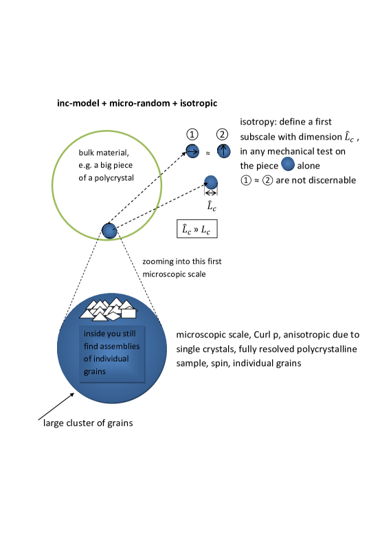
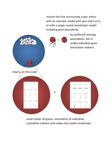
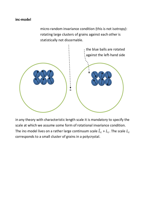
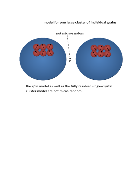
Figure 1: The micro-random model does not resolve a scale smaller than $\widehat{L}_{c}$ (blue-filled balls)! Inside the blue-filled balls, we have crystallites; if we want to model what happens inside there, we can still try to model this with isotropy assumption. This is our isotropic $\mbox{Curl}\,p$-model with spin (see Table 6). In reality however, the orientation of the crystallites matters.

Imagine a given initial distribution $F_{p}(x,0)$ of grains and subject the polycrystal to a given mechanical loading which alters the plastic state. The result will be recorded in the history $t\to F_{p}(x,t)$.

Now consider a randomly rotated initial distribution of grains and plastic distortions via

$$\boxed{\widetilde{F}_{p}(x,0):=Q(x)F_{p}(x,0)\quad\mbox{with}\quad Q(x)\in\operatorname{SO}(3)}\,.$$ (3.2)

At a sufficiently large scale we are not able to discern this rotational rearrangement and we are led to assume that the new plastic history under the same given loading as before should be

$$\boxed{t\to\widetilde{F}_{p}(x,t):=Q(x)F_{p}(x,t)}\,.$$ (3.3)

This is essentially a new invariance requirement to be imposed on our model for the polycrystal. It means that, up to the initially different inhomogeneous rotation of the grains, the response is the same. Since rotations are involved one might take this as a statement of classical isotropy. However, this would be misguided since classical isotropy is concerned with rigidly rotating the whole (polycrystalline) sample, while here each individual grain is rotated differently (see explanation in Figure 1).

Considering now the geometrically linear setting, we compare the initial infinitesimal plastic distortion $p(x,0)$ with solution $t\to p(x,t)$ versus $p(x,0)+A(x)$ with its time evolution $t\to\widetilde{p}(x,t)$. Our micro-randomness invariance condition postulates in the geometrically linear setting that

$$\boxed{\begin{array}[]{lllllll}p(x,0)&\to&\widetilde{p}(x,0)&=&p(x,0)&+&A(x)\quad\Rightarrow\\ p(x,t)&\to&\widetilde{p}(x,t)&=&p(x,t)&+&A(x)\quad\forall t>0\end{array}\quad\mbox{({\bf L}inear {\bf M}icro-{\bf R}andom)}}$$ (LMR)

and in the finite deformation setting that

$$\boxed{\begin{array}[]{lll}F_{p}(x,0)&\to&\widetilde{F}_{p}(x,0)=Q(x)\,F_{p}(x,0)\quad\Rightarrow\\ F_{p}(x,t)&\to&\widetilde{F}_{p}(x,t)=Q(x)\,F_{p}(x,t)\quad\forall t>0\end{array}\quad\mbox{({\bf F}inite {\bf M}icro-{\bf R}andom)}}$$ (FMR)

In addition, we are aware of the fact that determining exact initial conditions for the rotations of grains in a polycrystal is practically impossible. Therefore, the influence of considering different initial grain distributions should be minimized in order to obtain a suitable effective model. Our micro-randomness invariance condition ensures that the effect of different initial conditions shows only as an ”offset” of an otherwise unique response, as seen above.Notice that

$$\left.\begin{array}[]{lclcl}F(x)&=&F_{e}(x)\,F_{p}(x)&=&F_{e}(x)\underbrace{Q(x)^{T}Q(x)}_{=\,{\boldsymbol{\mathbbm{1}}}}F_{p}(x)\\ &&&&\\ \nabla u&=&e(x)+p(x)&=&e+\underbrace{A^{T}(x)+A(x)}_{=\,0}+p(x)\end{array}\right\}\,\qquad Q(x)=\exp(A(x))\,,$$ (3.4)

thus the invariance condition connected to micro-randomness reads in the finite strain case

$$(F,F_{e},F_{p})\quad\longrightarrow\quad(F,F_{e}Q^{T}(x),QF_{p}(x))\quad\forall\,Q(x)\in\operatorname{SO}(3)\,,$$ (3.5)

while in the geometrically linear context, we need to require the invariance

$$(\nabla u,e,p)\quad\longrightarrow\quad(\nabla u,e+A^{T}(x),A(x)+p(x))\quad\forall\,A(x)\in\operatorname{\mathfrak{so}}(3)\,.$$ (3.6)

3.3.  Isotropy in geometrically linear models

While the above invariance conditions can be characterized by additive operators, for classical isotropy we need the group of rotations $Q\in\operatorname{O}(3)$. We define isotropy in geometrically linear models to be form-invariance under simultaneous change of spatial and referential coordinates by a rigid rotation. In this case, scalar functions $h:\mathbb{R}^{3}\to\mathbb{R}$, vector fields $\phi:\mathbb{R}^{3}\to\mathbb{R}^{3}$ and second order tensor fields $S:\mathbb{R}^{3}\to\mathbb{R}^{3\times 3}$ are transformed as follows:

$$\left.\begin{array}[]{lclcl}h&\longrightarrow&h^{\sharp}&\mbox{with}&h^{\sharp}(\xi):=h(Q^{T}\xi)\,,\\ &&&&\\ \phi&\longrightarrow&\phi^{\sharp}&\mbox{with}&\phi^{\sharp}(\xi):=Q\,\phi(Q^{T}\xi)\,,\\ &&&&\\ S&\longrightarrow&S^{\sharp}&\mbox{with}&S^{\sharp}(\xi):=Q\,S(Q^{T}\xi)\,Q^{T}\,.\end{array}\right\}$$ (3.7)

It can be shown (see [94]) that

$$\operatorname{Curl\hskip 1.13791pt}_{\xi}\bigl{[}p^{\sharp}(\xi)\bigr{]}=Q\bigl{(}\operatorname{Curl\hskip 1.13791pt}_{x}p(x)\bigr{)}Q^{T}\qquad\mbox{ and }\qquad\operatorname{inc}_{\xi}\bigl{[}\operatorname{sym}p^{\sharp}(\xi)\bigr{]}=Q\,\operatorname{inc}_{x}\bigl{[}\operatorname{sym}p(x)\bigr{]}\,Q^{T}\,.$$ (3.8)

Therefore, both our incompatibility measures are properly isotropic and therefore all our presented models, based on $\operatorname{Curl\hskip 1.13791pt}p$ or $\operatorname{inc}(\operatorname{sym}p)$, respectively, are fully isotropic. A summary of the invariance conditions for infinitesimal gradient plasticity is presented in Table 3.

Objectivity/Linearized frame-indifference:	$\left\{\begin{array}[]{lcl}\nabla u&\longrightarrow&\overline{A}+\nabla u,\\ p&\longrightarrow&\overline{A}+p\end{array}\right.\quad\overline{A}\in\operatorname{\mathfrak{so}}(3)$
Linearized gauge-invariance:	$\left\{\begin{array}[]{lcl}\nabla u&\longrightarrow&\nabla u+\nabla\vartheta,\\ p&\longrightarrow&p+\nabla\vartheta\end{array}\right.\,\,\vartheta\in C^{\infty}(\mathbb{R}^{3},\mathbb{R}^{3})$
Linearized micro-randomness:	$\left.\begin{array}[]{lcl}\quad\,\,p&\longrightarrow&p+A(x)\end{array}\right.\quad A(x)\in\operatorname{\mathfrak{so}}(3)$
Isotropy:	$\left\{\begin{array}[]{lcll}h:\mathbb{R}^{3}\to\mathbb{R}&\longrightarrow&h^{\sharp}&\mbox{ with }h^{\sharp}(\xi):=h(Q^{T}\xi)\,,\\ \phi:\mathbb{R}^{3}\to\mathbb{R}^{3}&\longrightarrow&\phi^{\sharp}&\mbox{ with }\phi^{\sharp}(\xi):=Q\,\phi(Q^{T}\xi)\,,\\ S:\mathbb{R}^{3}\to\mathbb{R}^{3\times 3}&\longrightarrow&S^{\sharp}&\mbox{ with }S^{\sharp}(\xi):=Q\,S(Q^{T}\xi)\,Q^{T}\end{array}\right.\,Q\in\operatorname{O}(3)$

Table 3: Invariance conditions for infinitesimal gradient plasticity

4.  Some models of gradient plasticity with Kröner’s incompatibility tensor

Before we introduce and analyze our ”ideal” model designed from the set of requirements presented in the introduction, we found that it is more interesting to first present those few models we first considered with an emphasis on the difficulties and shortcomings of those models both from the mechanical and mathematical points of view. Let us first make it clear that the approach used to analyze those models as well as our model in Section 4.3 is trough a convex analytical framework and variational inequalities developed in Han-Reddy [62] for classical plasticity and quite often used for models of gradient plasticity (see [35, 123, 101, 38, 42]), as well.

4.1.  An irrotational model with linear kinematic hardening

In this section, we present a model with linear kinematic hardening and Kröner’s incompatibility tensor where the plastic variable is symmetric i.e., a model with no plastic spin. The goal is to find the displacement field $u$ and the infinitesimal plastic strain $\mbox{$\bf\varepsilon$}_{p}$ in some suitable function spaces such that the content of Table 4 holds.

Additive split of distortion:	$\nabla u=e+p$
Additive split of strain:	$\operatorname{sym}\nabla u=\mbox{$\bf\varepsilon$}_{e}+\mbox{$\bf\varepsilon$}_{p}$, $\mbox{$\bf\varepsilon$}_{e}:=\operatorname{sym}\,e\,\mbox{ and }\,\mbox{$\bf\varepsilon$}_{p}:=\operatorname{sym}p$
Equilibrium:	$\mbox{Div}\,\sigma+f=0$ with $\sigma=\mathbb{C}_{\mbox{\scriptsize{iso}}}\mbox{$\bf\varepsilon$}_{e}$
Free energy:	$\frac{1}{2}\,\langle\mathbb{C}_{\mbox{\scriptsize{iso}}}\mbox{$\bf\varepsilon$}_{e},\mbox{$\bf\varepsilon$}_{e}\rangle+\frac{1}{2}\,\mu\,k_{1}\,\left\lVert{\mbox{$\bf\varepsilon$}_{p}}\right\rVert^{2}+\frac{1}{2}\,\mu\,\widehat{L}^{4}_{c}\left\lVert{\operatorname{inc}(\mbox{$\bf\varepsilon$}_{p})}\right\rVert^{2}$
Yield condition:	$\phi(\Sigma_{E}):=\left\lVert{\operatorname{dev}\Sigma_{E}}\right\rVert-{\sigma}_{0}\leq 0$
where	$\Sigma_{E}:=\sigma+\Sigma_{\mbox{\scriptsize kin}}+\Sigma_{\mbox{\scriptsize inc}}$  with   $\Sigma_{\mbox{\scriptsize kin}}:=-\mu\,k_{1}\mbox{$\bf\varepsilon$}_{p}$,
	$\Sigma_{\mbox{\scriptsize inc}}:=-\mu\,\widehat{L}^{4}_{c}\operatorname{inc}(\operatorname{inc}\mbox{$\bf\varepsilon$}_{p})\in\mbox{Sym}(3)$
Dissipation inequality:	$\displaystyle\int_{\Omega}\langle\Sigma_{E},\dot{\mbox{$\bf\varepsilon$}}_{p}\rangle\,dx\geq 0$
Dissipation function:	$\mathcal{D}(q):={\sigma}_{0}\left\lVert{q}\right\rVert$
Flow law in primal form:	$\Sigma_{E}\in\partial\mathcal{D}(\dot{\mbox{$\bf\varepsilon$}}_{p})$
Flow law in dual form:	$\dot{\mbox{$\bf\varepsilon$}}_{p}=\lambda\,\displaystyle\frac{\operatorname{dev}\Sigma_{E}}{\left\lVert{\operatorname{dev}\Sigma_{E}}\right\rVert},\quad\qquad\lambda=\left\lVert{\dot{\mbox{$\bf\varepsilon$}}_{p}}\right\rVert$
KKT conditions:	$\lambda\geq 0$,  $\phi(\Sigma_{E})\leq 0$,  $\lambda\,\phi(\Sigma_{E})=0$
Boundary conditions for $\mbox{$\bf\varepsilon$}_{p}$:	to be specified
Function space for $\mbox{$\bf\varepsilon$}_{p}$:	$\mbox{$\bf\varepsilon$}_{p}(t,\cdot)\in L^{2}(\Omega,\mbox{Sym}(3))$ , $\operatorname{inc}(\mbox{$\bf\varepsilon$}_{p})\in L^{2}(\Omega,\mbox{Sym}(3))$

Table 4: The model with linear kinematic Prager-type hardening and Kröner’s incompatibility tensor. The boundary conditions on $\mbox{$\bf\varepsilon$}_{p}$ cannot be specified from the structure of the model. The problem with this model is the presence of the norm $\left\lVert{\varepsilon_{p}}\right\rVert^{2}$ which is not linearized gauge-invariant. A careful analysis of the model in the spirit of Section 4.3 will lead to single out the necessity of an $L^{2}$-control of $\operatorname{Curl\hskip 1.13791pt}\mbox{$\bf\varepsilon$}_{p}$, which is also not a priori controlled in the model. Altogether, well-posedness of the model remains unclear. A modified version of this model is presented in Table 5. This model is micro-random i.e., invariant w.r.t. $p\to p+A(x)$, $A(x)\in\operatorname{\mathfrak{so}}(3)$, but not linearized gauge-invariant, i.e., not invariant w.r.t. $p\to p+\nabla\vartheta$,  $\vartheta\in C^{\infty}(\mathbb{R}^{3},\mathbb{R})$.

Additive split of distortion:	$\nabla u=e+p$
Additive split of strain:	$\operatorname{sym}\nabla u=\mbox{$\bf\varepsilon$}_{e}+\mbox{$\bf\varepsilon$}_{p}$, $\mbox{$\bf\varepsilon$}_{e}:=\operatorname{sym}\,e\,\mbox{ and }\,\mbox{$\bf\varepsilon$}_{p}:=\operatorname{sym}p$
Equilibrium:	$\mbox{Div}\,\sigma+f=0$ with $\sigma=\mathbb{C}_{\mbox{\scriptsize{iso}}}\mbox{$\bf\varepsilon$}_{e}$
Free energy:	$\frac{1}{2}\,\langle\mathbb{C}_{\mbox{\scriptsize{iso}}}\mbox{$\bf\varepsilon$}_{e},\mbox{$\bf\varepsilon$}_{e}\rangle+\frac{1}{2}\,\mu\,k_{1}\,\left\lVert{\mbox{$\bf\varepsilon$}_{p}}\right\rVert^{2}+\frac{1}{2}\,\mu\,L_{c}^{2}\,\left\lVert{\operatorname{Curl\hskip 1.13791pt}\mbox{$\bf\varepsilon$}_{p}}\right\rVert^{2}+\frac{1}{2}\,\mu\,\widehat{L}^{4}_{c}\left\lVert{\operatorname{inc}(\mbox{$\bf\varepsilon$}_{p})}\right\rVert^{2}$
Yield condition:	$\phi(\Sigma_{E}):=\left\lVert{\operatorname{dev}\Sigma_{E}}\right\rVert-{\sigma}_{0}\leq 0$
where	$\begin{array}[]{lcl}\Sigma_{E}&:=&\sigma+\Sigma_{\mbox{\scriptsize kin}}+\Sigma_{\mbox{\scriptsize curl}}+\Sigma_{\mbox{\scriptsize inc}}\,,\qquad\Sigma_{\mbox{\scriptsize kin}}:=-\mu\,k_{1}\mbox{$\bf\varepsilon$}_{p}\\ \Sigma_{\mbox{\scriptsize curl}}&:=&-\mu\,L^{2}_{c}\operatorname{sym}\operatorname{Curl\hskip 1.13791pt}\operatorname{sym}\operatorname{Curl\hskip 1.13791pt}\mbox{$\bf\varepsilon$}_{p}\in\mbox{Sym}(3)\\ \Sigma_{\mbox{\scriptsize inc}}&:=&-\mu\,\widehat{L}^{4}_{c}\operatorname{inc}(\operatorname{inc}\mbox{$\bf\varepsilon$}_{p})\in\mbox{Sym}(3)\end{array}$
Dissipation inequality:	$\displaystyle\int_{\Omega}\langle\Sigma_{E},\dot{\mbox{$\bf\varepsilon$}}_{p}\rangle\,dx\geq 0$
Dissipation function:	$\mathcal{D}(q):={\sigma}_{0}\left\lVert{q}\right\rVert$
Flow law in primal form:	$\Sigma_{E}\in\partial\mathcal{D}(\dot{\mbox{$\bf\varepsilon$}}_{p})$
Flow law in dual form:	$\dot{\mbox{$\bf\varepsilon$}}_{p}=\lambda\,\displaystyle\frac{\operatorname{dev}\Sigma_{E}}{\left\lVert{\operatorname{dev}\Sigma_{E}}\right\rVert},\quad\qquad\lambda=\left\lVert{\dot{\mbox{$\bf\varepsilon$}}_{p}}\right\rVert$
KKT conditions:	$\lambda\geq 0$,  $\phi(\Sigma_{E})\leq 0$,  $\lambda\,\phi(\Sigma_{E})=0$
Boundary conditions for $\mbox{$\bf\varepsilon$}_{p}$:	$\mbox{$\bf\varepsilon$}_{p}\times n|_{\partial\Omega}=0\quad\mbox{ and }\quad(\operatorname{Curl\hskip 1.13791pt}\mbox{$\bf\varepsilon$}_{p})^{T}\times n|_{\partial\Omega}=0$
Function space for $\mbox{$\bf\varepsilon$}_{p}$:	$\mbox{$\bf\varepsilon$}_{p}(t,\cdot)\in L^{2}(\Omega,\mbox{Sym}(3))$ , $\operatorname{inc}(\mbox{$\bf\varepsilon$}_{p})\in L^{2}(\Omega,\mbox{Sym}(3))$

Table 5: The model with linear kinematic Prager-type hardening and Kröner’s incompatibility tensor. The simple regularization term $\left\lVert{\operatorname{Curl\hskip 1.13791pt}\mbox{$\bf\varepsilon$}_{p}}\right\rVert^{2}$ allows to justify the boundary conditions on $\mbox{$\bf\varepsilon$}_{p}$. The problem with this model is the presence of the norms $\left\lVert{\varepsilon_{p}}\right\rVert^{2}$ and $\left\lVert{\operatorname{Curl\hskip 1.13791pt}\mbox{$\bf\varepsilon$}_{p}}\right\rVert^{2}$ which are both not linearized gauge-invariant. Altogether, well-posedness of this modified model is obtained as in Section 4.3, with the difference that uniqueness of the weak solution is obtained without any additional regularity assumption. This model is micro-random i.e., invariant w.r.t. $p\to p+A(x)$, $A(x)\in\operatorname{\mathfrak{so}}(3)$, but not linearized gauge-invariant, i.e., not invariant w.r.t. $p\to p+\nabla\vartheta$, $\vartheta\in C^{\infty}(\mathbb{R}^{3},\mathbb{R})$.

4.2.  A fully isotropic model with isotropic hardening and plastic spin

The model is completely described in Table 6.

Additive split of distortion:	$\nabla u=e+p$, $\mbox{$\bf\varepsilon$}_{e}=\mbox{sym}\,e$, $\mbox{$\bf\varepsilon$}_{p}=\operatorname{sym}p$
Equilibrium:	$\mbox{Div}\,\sigma+f=0$ with $\sigma=\mathbb{C}_{\mbox{\scriptsize{iso}}}\mbox{$\bf\varepsilon$}_{e}$
Free energy:	$\displaystyle\frac{1}{2}\,\langle\mathbb{C}_{\mbox{\scriptsize{iso}}}\mbox{$\bf\varepsilon$}_{e},\mbox{$\bf\varepsilon$}_{e}\rangle+\frac{1}{2}\,\mu\,k_{2}\,|\widetilde{\gamma}_{p}|^{2}+\,\,\frac{1}{2}\,\mu\,L^{2}_{c}\left\lVert{\operatorname{Curl\hskip 1.13791pt}p}\right\rVert^{2}$
Yield condition:	$\phi(\Sigma_{E},g):=\left\lVert{\operatorname{dev}\Sigma_{E}}\right\rVert-({\sigma}_{0}-g)\leq 0$ where  $g:=-\mu\,k_{2}\widetilde{\gamma}_{p}$
	$\begin{array}[]{lcl}\Sigma_{E}&:=&\sigma+\Sigma_{\mbox{\scriptsize curl}}\,,\\ \Sigma_{\mbox{\scriptsize curl}}&:=&-\,\mu\,L^{2}_{c}\,\operatorname{Curl\hskip 1.13791pt}\operatorname{Curl\hskip 1.13791pt}p\end{array}$
Dissipation inequality:	$\displaystyle\int_{\Omega}\bigl{[}\langle\Sigma_{E},\dot{p}\rangle+g\,\dot{\widetilde{\gamma}}_{p}\rangle\bigr{]}\,dx\geq 0$
Dissipation function:	$\mathcal{D}(\dot{\mbox{$\bf\varepsilon$}}_{p},\dot{\widetilde{\gamma}}_{p}):=\left\{\begin{array}[]{ll}\left\lVert{\dot{p}}\right\rVert&\mbox{ if }\left\lVert{\dot{p}}\right\rVert\leq\dot{\widetilde{\gamma}}_{p},\\ \infty&\mbox{ otherwise}\end{array}\right.$
Flow law in primal form:	$(\Sigma_{E},g)\in\partial\mathcal{D}(\dot{\mbox{$\bf\varepsilon$}}_{p},\dot{\widetilde{\gamma}}_{p})$
Flow law in dual form:	$\dot{p}=\lambda\,\displaystyle\frac{\operatorname{dev}\Sigma_{E}}{\left\lVert{\operatorname{dev}\Sigma_{E}}\right\rVert},\quad\quad\dot{\widetilde{\gamma}}_{p}=\lambda=\left\lVert{\dot{p}}\right\rVert$
KKT conditions:	$\lambda\geq 0$,  $\phi(\Sigma_{E},g)\leq 0$,  $\lambda\,\phi(\Sigma_{E},g)=0$
Boundary conditions for $p$:	$p\times n|_{\Gamma}=0$, $\operatorname{Curl\hskip 1.13791pt}p\times n|_{\partial\Omega\setminus\Gamma}=0$

Table 6: A fully isotropic model with isotropic hardening and plastic spin. The model is fully isotropic since it is form-invariant under the $\sharp$-transformation defined in (3.7). The model is also linearized gauge-invariant i.e., invariant w.r.t. $p\to p+\nabla\vartheta$, $\vartheta\in C^{\infty}(\mathbb{R}^{3},\mathbb{R})$, but not micro-random i.e., not invariant w.r.t. $p\to p+A(x)$, $A(x)\in\operatorname{\mathfrak{so}}(3)$.

4.3.  An irrotational model with isotropic hardening

In this section we discuss a variant of the previous model with linear kinematic hardening replaced by isotropic hardening. The new model will be invariant under Linear Referential Isotropy (LRIso), Linear Micro-Random (LMR), Linear Gauge-Invariance (LGI), Linear Elastic Objectivity, Linear Elastic Isotropy.

4.3.1.  Derivation of the model

The balance equation. The conventional macroscopic force balance leads to the equation of equilibrium

$$\operatorname{Div}\sigma+f=0$$ (4.1)

in which $\sigma$ is the infinitesimal symmetric Cauchy stress and $f$ is the body force.Constitutive equations. The constitutive equations are obtained from a free energy imbalance together with a flow law that characterizes plastic behaviour. The total strain $\bf\varepsilon$ is additively decomposed into elastic and plastic components $\mbox{$\bf\varepsilon$}_{e}$ and $\mbox{$\bf\varepsilon$}_{p}$, so that

$$\mbox{$\bf\varepsilon$}=\mbox{$\bf\varepsilon$}_{e}+\mbox{$\bf\varepsilon$}_{p}$$ (4.2)

with the plastic strain incapable of sustaining volumetric changes; that is, $\mbox{tr}\,\mbox{$\bf\varepsilon$}_{p}=0\,.$
The strain-displacement relation is given by

$$\mbox{$\bf\varepsilon$}=\operatorname{sym}\nabla u=\frac{1}{2}(\nabla u+\nabla u^{T})\,.$$ (4.3)

Free energy density: In this model the free-energy density is considered in the additively separated form

$$\mbox{W}(u,\varepsilon_{p},\operatorname{inc}\varepsilon_{p},\gamma_{p}): = \underbrace{\mbox{W}_{e}(\mbox{$\bf\varepsilon$}_{e})}_{\mbox{\footnotesize elastic energy}}\,\,+\,\,\underbrace{\mbox{W}_{\mbox{\scriptsize inc}}(\operatorname{inc}\varepsilon_{p})}_{\begin{array}[]{c}\mbox{\footnotesize mesoscopic}\\ \mbox{\footnotesize incompatibility}\end{array}}\,\,+\,\,\underbrace{\mbox{W}_{\mbox{\scriptsize iso}}(\gamma_{p})}_{\begin{array}[]{c}\mbox{\footnotesize isotropic hardening}\\ \mbox{\footnotesize energy (SSD-related)}\end{array}}\,,$$ (4.8)

where

$$\left.\begin{array}[]{lll}\mbox{W}_{\mbox{\footnotesize e}}(\mbox{$\bf\varepsilon$}_{e})&:=&\displaystyle\frac{1}{2}\,\langle\mbox{$\bf\varepsilon$}_{e},\mathbb{C}_{\mbox{\scriptsize{iso}}}\mbox{$\bf\varepsilon$}_{e}\rangle=\mu\,\left\lVert{\operatorname{sym}\nabla u-\varepsilon_{p}}\right\rVert^{2}+\frac{1}{2}\,\lambda\operatorname{tr}[\nabla u-\varepsilon_{p}]^{2}\,,\\ \\ \mbox{W}_{\mbox{\scriptsize inc}}(\operatorname{inc}\varepsilon_{p})&:=&\displaystyle\frac{1}{2}\,\mu\,\widehat{L}^{4}_{c}\left\lVert{\operatorname{inc}\varepsilon_{p}}\right\rVert^{2}=\frac{1}{2}\mu\,\widehat{L}^{4}_{c}\left\lVert{\operatorname{Curl\hskip 1.13791pt}[(\operatorname{Curl\hskip 1.13791pt}\varepsilon_{p})^{T}]}\right\rVert^{2},\\ \\ \mbox{W}_{\mbox{\scriptsize iso}}(\gamma_{p})&:=&\displaystyle\frac{1}{2}\,\mu\,k_{2}\,|\gamma_{p}|^{2}\,,\end{array}\right\}$$ (4.9)

and $\lambda,\,\mu$ are the Lamé moduli with $\mu>0$ and $3\lambda+2\mu>0$, $\widehat{L}_{c}\geq 0$ is an energetic length scale and $k_{2}\geq 0$ is a positive non-dimensional isotropic hardening constant, $\gamma_{p}$ is the isotropic hardening variable (the accumulated equivalent plastic strain).From the local free energy inbalance

$$\frac{\rm d}{\rm dt}\mbox{W}\leq\langle\sigma,\nabla u_{t}\rangle=\langle\sigma,\dot{\mbox{$\bf\varepsilon$}}\rangle \Leftrightarrow \frac{\rm d}{\rm dt}\mbox{W}-\langle\sigma,\dot{\varepsilon}_{e}\rangle-\langle\sigma,\dot{\varepsilon}_{p}\rangle\leq 0$$

$$\Leftrightarrow \frac{\rm d}{\rm dt}{\rm W}(u,\varepsilon_{p},\mbox{D}^{2}\varepsilon_{p},\gamma_{p})\leq 0\quad\mbox{ for $u$ fixed}$$

where the second equivalence is obtained using arguments from thermodynamics which give the elasticity relation

$$\sigma={\mathbb{C}}_{\mbox{\scriptsize{iso}}}\mbox{$\bf\varepsilon$}_{e}=2\mu\,(\operatorname{sym}\nabla u-\mbox{$\bf\varepsilon$}_{p})+\lambda\,\operatorname{tr}(\operatorname{sym}\nabla u-\mbox{$\bf\varepsilon$}_{p}){\boldsymbol{\mathbbm{1}}}\,.$$ (4.10)

Therefore, we get

$$\langle\sigma,\dot{\varepsilon}_{p}\rangle-\mu\,\widehat{L}^{4}_{c}\langle\operatorname{inc}\varepsilon_{p},\operatorname{inc}\dot{\varepsilon}_{p}\rangle-\mu\,k_{2}\,\gamma_{p}\,\dot{\gamma}_{p}\geq 0\,.$$ (4.11)

Now, integrating (4.11), we arrive at

$$0 \leq \int_{\Omega}\Bigl{[}\langle\sigma,\dot{\mbox{$\bf\varepsilon$}}_{p}\rangle-\mu\,\widehat{L}_{c}^{4}\,\langle\,\underbrace{\operatorname{inc}(\operatorname{inc}\mbox{$\bf\varepsilon$}_{p})}_{\in\mbox{Sym}(3)},\dot{\mbox{$\bf\varepsilon$}}_{p}\rangle-\mu\,k_{2}\,\gamma_{p}\,\dot{\gamma}_{p}-\sum_{i=1}^{3}\mathop{\rm div}\nolimits\Bigl{(}\mu\,\widehat{L}_{c}^{4}\,\dot{\mbox{$\bf\varepsilon$}}_{p\,i}\times\bigl{[}\operatorname{Curl\hskip 1.13791pt}\operatorname{inc}\mbox{$\bf\varepsilon$}_{p}\bigr{]}^{T}_{i}\Bigr{)}$$

$$\hskip 42.67912pt-\sum_{i=1}^{3}\mathop{\rm div}\nolimits\Bigl{(}\mu\,\widehat{L}_{c}^{4}\,\bigl{[}\operatorname{Curl\hskip 1.13791pt}\dot{\mbox{$\bf\varepsilon$}}_{p}\bigr{]}^{T}_{i}\times\bigl{[}\operatorname{inc}\mbox{$\bf\varepsilon$}_{p}\bigr{]}_{i}\Bigr{)}\Bigr{]}\,dx$$

$$= \int_{\Omega}\Bigl{[}\langle\sigma-\mu\,\widehat{L}_{c}^{4}\,\operatorname{inc}(\operatorname{inc}\mbox{$\bf\varepsilon$}_{p}),\dot{\varepsilon}_{p}\rangle-\mu\,k_{2}\,\gamma_{p}\,\dot{\gamma}_{p}\Bigr{]}dx$$

$$\hskip 28.45274pt-\sum_{i=1}^{3}\mu\,\widehat{L}_{c}^{4}\int_{\partial\Omega}\langle\dot{\mbox{$\bf\varepsilon$}}_{p\,i}\times\bigl{[}\operatorname{Curl\hskip 1.13791pt}\operatorname{inc}\mbox{$\bf\varepsilon$}_{p}\bigr{]}^{T}_{i},n\rangle\,dS-\sum_{i=1}^{3}\mu\,\widehat{L}_{c}^{4}\int_{\partial\Omega}\langle\bigl{[}\operatorname{Curl\hskip 1.13791pt}\dot{\mbox{$\bf\varepsilon$}}_{p}\bigr{]}^{T}_{i}\times\bigl{[}\operatorname{inc}\mbox{$\bf\varepsilon$}_{p}\bigr{]}_{i},n\rangle\,dS\,.$$

In order to obtain a global reduced dissipation inequality one needs to choose suitable boundary conditions for which the two equations below are satisfied

$$\sum_{i=1}^{3}\int_{\partial\Omega}\langle\dot{\mbox{$\bf\varepsilon$}}_{p\,i}\times n,\bigl{[}\operatorname{Curl\hskip 1.13791pt}\operatorname{inc}\mbox{$\bf\varepsilon$}_{p}\bigr{]}^{T}_{i}\rangle\,dS = 0\,.$$ (4.13)

$$\sum_{i=1}^{3}\int_{\partial\Omega}\langle\bigl{[}\operatorname{Curl\hskip 1.13791pt}\dot{\mbox{$\bf\varepsilon$}}_{p}\bigr{]}^{T}_{i}\times n,\bigl{[}\operatorname{inc}\mbox{$\bf\varepsilon$}_{p}\bigr{]}_{i}\rangle\,dS = 0\,.$$ (4.14)

The simplest lower order boundary conditions to satisfy (4.13) and (4.14) are

$$\varepsilon_{p}\times n|_{\partial\Omega}=0\qquad\mbox{ and }\qquad\bigl{[}\operatorname{Curl\hskip 1.13791pt}\varepsilon_{p}\bigr{]}^{T}\times n|_{\partial\Omega}=0\,.$$ (4.15)

Other possible boundary conditions to satisfy the equations (4.13) and (4.14) are given in the table below.

boundary conditions for (4.13)	boundary conditions for (4.14)
$[\operatorname{Curl\hskip 1.13791pt}\operatorname{inc}\mbox{$\bf\varepsilon$}_{p}\bigr{]}^{T}\times n|_{\partial\Omega}=0$	$(\operatorname{inc}\varepsilon_{p})\times n|_{\partial\Omega}=0$
$\varepsilon_{p}\times n|_{\Gamma}=0\quad\mbox{ and }\quad\bigl{[}\operatorname{Curl\hskip 1.13791pt}\operatorname{inc}\varepsilon_{p}\bigr{]}^{T}\times n|_{\partial\Omega\setminus\Gamma}=0$	$\bigl{[}\operatorname{Curl\hskip 1.13791pt}\varepsilon_{p}\bigr{]}^{T}\times n|_{\Gamma}=0\quad\mbox{ and }\quad\operatorname{inc}\mbox{$\bf\varepsilon$}_{p}\times n|_{\partial\Omega\setminus\Gamma}=0$ .

Table 7: Possible boundary conditions for (4.13) and (4.14) to be satisfied.

However, these boundary conditions cannot be mathematically justified from the free-energy density W considered so far: both terms in (4.13) and (4.14) are not automatically well-defined as boundary traces. In fact, one needs to show that $\mbox{$\bf\varepsilon$}_{p}\in\mbox{H}(\mbox{Curl})$ and $(\operatorname{Curl\hskip 1.13791pt}\mbox{$\bf\varepsilon$}_{p})^{T}\in\mbox{H}(\mbox{Curl})$. This information is missing from the energy. We only know that $\mbox{$\bf\varepsilon$}_{p}\in\mbox{L}^{2}$ (due to isotropic hardening) and $\operatorname{inc}\mbox{$\bf\varepsilon$}_{p}=\operatorname{Curl\hskip 1.13791pt}[(\operatorname{Curl\hskip 1.13791pt}\mbox{$\bf\varepsilon$}_{p})^{T}]\in\mbox{L}^{2}$. The missing piece of information to proceed is $\operatorname{Curl\hskip 1.13791pt}\mbox{$\bf\varepsilon$}_{p}\in\mbox{L}^{2}$.

So, one needs to modify the model by adding a new regularizing term in the free-energy density $W$, which is physically meaningful in the sense that it does satisfy some invariance properties. The unmodified model is summarized in Table 8.

Additive split of strain:	$\operatorname{sym}\nabla u=\mbox{$\bf\varepsilon$}_{e}+\mbox{$\bf\varepsilon$}_{p}$
Equilibrium:	$\mbox{Div}\,\sigma+f=0$ with $\sigma=\mathbb{C}_{\mbox{\scriptsize{iso}}}\mbox{$\bf\varepsilon$}_{e}$
Free energy:	$\displaystyle\frac{1}{2}\,\langle\mathbb{C}_{\mbox{\scriptsize{iso}}}\mbox{$\bf\varepsilon$}_{e},\mbox{$\bf\varepsilon$}_{e}\rangle+\frac{1}{2}\,\mu\,k_{2}\,|\gamma_{p}|^{2}+\,\frac{1}{2}\,\mu\,\widehat{L}^{4}_{c}\left\lVert{\operatorname{inc}\mbox{$\bf\varepsilon$}_{p}}\right\rVert^{2}$
Yield condition:	$\phi(\Sigma_{E},g):=\left\lVert{\operatorname{dev}\Sigma_{E}}\right\rVert-({\sigma}_{0}-g)\leq 0$ where  $g:=-\mu\,k_{2}\gamma_{p}$
	$\begin{array}[]{lcl}\Sigma_{E}&:=&\sigma+\Sigma_{\mbox{\scriptsize inc}}\,,\\ \Sigma_{\mbox{\scriptsize inc}}&:=&-\mu\,\widehat{L}^{4}_{c}\,\operatorname{inc}\operatorname{inc}\mbox{$\bf\varepsilon$}_{p}\,=\,\operatorname{Curl\hskip 1.13791pt}\Bigl{(}\bigl{[}\operatorname{Curl\hskip 1.13791pt}\operatorname{Curl\hskip 1.13791pt}[(\operatorname{Curl\hskip 1.13791pt}\mbox{$\bf\varepsilon$}_{p})^{T}]\bigr{]}^{T}\Bigr{)}\end{array}$
Dissipation inequality:	$\displaystyle\int_{\Omega}\bigl{[}\langle\Sigma_{E},\dot{\mbox{$\bf\varepsilon$}}_{p}\rangle+g\,\dot{\gamma}_{p}\rangle\bigr{]}\,dx\geq 0$
Dissipation function:	$\mathcal{D}(\dot{\mbox{$\bf\varepsilon$}}_{p},\dot{\gamma}_{p}):=\left\{\begin{array}[]{ll}{\sigma}_{0}\,\left\lVert{\dot{\mbox{$\bf\varepsilon$}}_{p}}\right\rVert&\mbox{ if }\left\lVert{\dot{\mbox{$\bf\varepsilon$}}_{p}}\right\rVert\leq\dot{\gamma}_{p},\\ \infty&\mbox{ otherwise}\end{array}\right.$
Flow law in primal form:	$(\Sigma_{E},g)\in\partial\mathcal{D}(\dot{\mbox{$\bf\varepsilon$}}_{p},\dot{\gamma}_{p})$
Flow law in dual form:	$\dot{\mbox{$\bf\varepsilon$}}_{p}=\lambda\,\displaystyle\frac{\operatorname{dev}\Sigma_{E}}{\left\lVert{\operatorname{dev}\Sigma_{E}}\right\rVert},\quad\quad\dot{\gamma}_{p}=\lambda=\left\lVert{\dot{\mbox{$\bf\varepsilon$}}_{p}}\right\rVert$
KKT conditions:	$\lambda\geq 0$,  $\phi(\Sigma_{E},g)\leq 0$,  $\lambda\,\phi(\Sigma_{E},g)=0$
Boundary conditions for $\mbox{$\bf\varepsilon$}_{p}$:	$\mbox{$\bf\varepsilon$}_{p}\times n|_{\partial\Omega}=0\,,\quad(\operatorname{Curl\hskip 1.13791pt}\mbox{$\bf\varepsilon$}_{p})^{T}\times n|_{\partial\Omega}=0$

Table 8: The irrotational model with isotropic hardening and Kröner’s incompatibility tensor. The terms in the free-energy density are not enough to guarantee the minimum regularity required, i.e., $\mbox{$\bf\varepsilon$}_{p}\in\mbox{H}(\mbox{Curl})$ and $(\operatorname{Curl\hskip 1.13791pt}\mbox{$\bf\varepsilon$}_{p})^{T}\in\mbox{H}(\mbox{Curl})$, in order to justify mathematically the boundary conditions $\mbox{$\bf\varepsilon$}_{p}\times n|_{\partial\Omega}=0$ and $(\operatorname{Curl\hskip 1.13791pt}\mbox{$\bf\varepsilon$}_{p})^{T}\times n|_{\partial\Omega}=0$.

We will consider the additional term

$$\mbox{W}_{\mbox{\scriptsize curl}}(\operatorname{Curl\hskip 1.13791pt}p):=\displaystyle\frac{1}{2}\,\mu\,L_{c}^{2}\,\left\lVert{\operatorname{dev}\operatorname{sym}\operatorname{Curl\hskip 1.13791pt}\mbox{$\bf\varepsilon$}_{p}}\right\rVert^{2}\,,$$ (4.16)

which is motivated in the following section.

4.3.2.  Conformal gauge-invariance - the regularization term $\mathbf{\operatorname{dev}}\operatorname{sym}\operatorname{Curl\hskip 1.13791pt}\mbox{$\bf\varepsilon$}_{p}$

We will see subsequently that the model with the regularizing term $\operatorname{dev}\operatorname{sym}\operatorname{Curl\hskip 1.13791pt}\mbox{$\bf\varepsilon$}_{p}$ allows for a mathematical existence proof. However, what about the invariance conditions, notably gauge-invariance?
It is easy to see that

$$p\to\operatorname{dev}\operatorname{sym}\operatorname{Curl\hskip 1.13791pt}\mbox{$\bf\varepsilon$}_{p}=\operatorname{dev}\operatorname{sym}\operatorname{Curl\hskip 1.13791pt}\operatorname{sym}p$$

is micro-random while it is not linear gauge-invariant, i.e.,

$$\begin{array}[]{rcl}p&\to&p+\nabla\vartheta\\ \operatorname{dev}\operatorname{sym}\operatorname{Curl\hskip 1.13791pt}\operatorname{sym}(\nabla\vartheta+p)&\neq&\operatorname{dev}\operatorname{sym}\operatorname{Curl\hskip 1.13791pt}\operatorname{sym}p,\quad\forall\vartheta\in C^{1}(\Omega,\mathbb{R}^{3})\,.\end{array}$$ (4.17)

Let us now determine those mappings $\vartheta:\mathbb{R}^{3}\to\mathbb{R}^{3}$ which are still “allowed” for gauge-invariance, in the sense that

$$\operatorname{dev}\operatorname{sym}\operatorname{Curl\hskip 1.13791pt}\operatorname{sym}(\nabla\vartheta+p)\,=\,\operatorname{dev}\operatorname{sym}\operatorname{Curl\hskip 1.13791pt}\operatorname{sym}p\,.$$

Automatically, these mappings satisfy the identity $\operatorname{inc}(\operatorname{sym}\nabla\vartheta)=0$. Moreover, by linearity we should have

$$\operatorname{dev}\operatorname{sym}\operatorname{Curl\hskip 1.13791pt}\operatorname{sym}\nabla\vartheta=0\,.$$ (4.18)

Since, however, $\operatorname{tr}(\operatorname{Curl\hskip 1.13791pt}S)=0$ for all smooth symmetric tensor fields $S\in\mbox{Sym}(3)$ (see (5.3) in the appendix), the latter is equivalent to

$$\operatorname{sym}\operatorname{Curl\hskip 1.13791pt}\operatorname{sym}\nabla\vartheta=0\,.$$

This implies that for some non-constant skew-symmetric tensor field $A:\Omega\to\operatorname{\mathfrak{so}}(3)$ we have

$$\operatorname{Curl\hskip 1.13791pt}\operatorname{sym}\nabla\vartheta(x)=A(x)\quad\Leftrightarrow\quad(\operatorname{Curl\hskip 1.13791pt}\operatorname{sym}\nabla\vartheta)^{T}=-A(x)\,.$$ (4.19)

Taking the Curl on both sides leads to

$$\operatorname{Curl\hskip 1.13791pt}[(\operatorname{Curl\hskip 1.13791pt}\operatorname{sym}\nabla\vartheta)^{T}]=-\operatorname{Curl\hskip 1.13791pt}A(x)\quad\Leftrightarrow\quad 0\,=\,\operatorname{inc}(\operatorname{sym}\nabla\vartheta)\,=-\,\operatorname{Curl\hskip 1.13791pt}A(x)\,.$$ (4.20)

Thus, $A(x)=\overline{A}$ is a constant skew-symmetric matrx, according to an observation in [94]. Reinserting into (4.19), we must have

$$\operatorname{Curl\hskip 1.13791pt}\operatorname{sym}\nabla\vartheta(x)=\overline{A}\,.$$ (4.21)

We observe that (see [104])

$$\operatorname{Curl\hskip 1.13791pt}(\zeta(x_{1},x_{2},x_{3})\cdot{\boldsymbol{\mathbbm{1}}})=\left(\begin{array}[]{ccc}0&-\zeta_{,3}&\zeta_{,2}\\ \zeta_{,3}&0&-\zeta_{,1}\\ -\zeta_{,2}&\zeta_{,1}&0\end{array}\right)\,\quad\zeta:\mathbb{R}^{3}\to\mathbb{R}\,$$

and with $\zeta(x_{1},x_{2},x_{3})=a\,x_{1}+b\,x_{2}+c\,x_{3}$, we obtain

$$\operatorname{Curl\hskip 1.13791pt}((ax_{1}+bx_{2}+cx_{3})\cdot{\boldsymbol{\mathbbm{1}}})=\left(\begin{array}[]{ccc}0&-c&b\\ c&0&-a\\ -b&a&0\end{array}\right)\,.$$

Hence, a solution to (4.21) can be obtained in the format

$$\operatorname{sym}\nabla\vartheta(x_{1},x_{2},x_{3})=\zeta(x_{1},x_{2},x_{3})\cdot{\boldsymbol{\mathbbm{1}}}\,.$$ (4.22)

On taking again the deviatoric part of the latter we arrive at

$$\operatorname{dev}\operatorname{sym}\nabla\vartheta(x_{1},x_{2},x_{3})=0\,.$$ (4.23)

This is equivalent to

$$\nabla\vartheta(x)=\zeta(x_{1},x_{2},x_{3})\cdot{\boldsymbol{\mathbbm{1}}}+A(x_{1},x_{2},x_{3})\quad\mbox{ with }\quad A:\mathbb{R}^{3}\to\operatorname{\mathfrak{so}}(3)\,.$$ (4.24)

The solution to (4.23) can be given in closed form. In fact, taking Curl on both sides of (4.24), together with the fact that $\operatorname{Curl\hskip 1.13791pt}(\zeta(x_{1},x_{2},x_{3})\cdot{\boldsymbol{\mathbbm{1}}})\in\operatorname{\mathfrak{so}}(3)$ one gets $A(x_{1},x_{2},x_{3})=\widehat{A}\in\operatorname{\mathfrak{so}}(3)$ constant skew-symmetric matrix. Also, using the operators axl and anti defined in (2.5), a general solution to (4.23) is obtained in the form

$$\phi_{c}(x):=\frac{1}{2}\,\Bigl{(}2\langle\operatorname{axl}\bigl{(}\widehat{W}\bigr{)},x\rangle\,x-\operatorname{axl}\bigl{(}\widehat{W}\bigr{)}\,\left\lVert{x}\right\rVert^{2}\Bigr{)}+\bigl{[}\widehat{\zeta}\cdot{\boldsymbol{\mathbbm{1}}}+\widehat{A}\bigr{]}\,x+\widehat{\eta}\,,$$ (4.25)

where $\widehat{A},\,\widehat{W}\in\operatorname{\mathfrak{so}}(3)$ are arbitrary constant skew-symmetric matrices and $\widehat{\zeta},\,\widehat{\eta}\in\mathbb{R}^{3}$ are arbitrary constant vectors.
The mappings in (4.25) are called infinitesimal conformal mappings $\phi_{c}$ (see [106]). The mappings $x\to\phi_{c}(x)$ locally preserve the shape of infinitesimal cubes but are globally inhomogeneous.

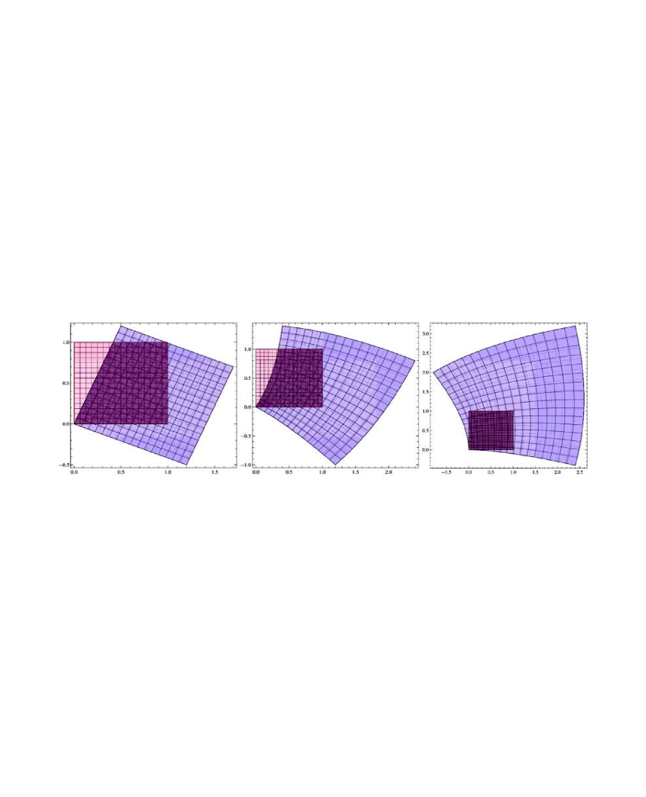
Figure 2: Infinitesimal conformal mappings $\phi_{c}:\mathbb{R}^{3}\to\mathbb{R}^{3}$ which locally leave shapes invariant: a prototype elastic deformation in the sense that the corresponding stress deviator $\operatorname{dev}\sigma(\nabla\phi_{c})=0$. Shown is the coarse grid deformation. The picture is extracted from [106].

If we consider $x\to\phi_{c}(x)$ as elastic displacement, then, according to the von Mises $J_{2}$-criterion, these mappings alone never lead to plasticity since

$$\operatorname{dev}\sigma=\operatorname{dev}\bigl{(}2\,\mu\,\operatorname{sym}\nabla\phi_{c}+\lambda\,\operatorname{tr}(\nabla\phi_{c}\cdot{\boldsymbol{\mathbbm{1}}}\bigr{)}=2\,\mu\operatorname{dev}\operatorname{sym}\nabla\phi_{c}=0\,.$$

Gathering our findings, we have obtained that the regularization term (4.16) is invariant w.r.t. the infinitesimal conformal group and infinitesimal conformal mappings $\phi_{c}$ do not induce irreversible processes.

There is still another solution to

$$\operatorname{sym}\operatorname{Curl\hskip 1.13791pt}\operatorname{sym}\nabla\vartheta=0\,.$$ (4.26)

Clearly, (4.26) will be satisfied also if already

$$\operatorname{Curl\hskip 1.13791pt}\operatorname{sym}\nabla\vartheta=0\,,$$

which in turn is satsfied for $\operatorname{sym}\nabla\vartheta=\nabla v\in\mbox{Sym}(3)$, with $v:\mathbb{R}^{3}\to\mathbb{R}^{3}$. Such a vector can be taken as $v=\nabla h(x_{1},x_{2},x_{3})$ with any scalar function $h:\mathbb{R}^{3}\to\mathbb{R}$. Then, (4.26) is satisfied. Thus, another solution to (4.26) is given by

$$\vartheta(x_{1},x_{2},x_{3})=\nabla h(x_{1},x_{2},x_{3}),\quad h:\mathbb{R}^{3}\to\mathbb{R}\,.$$

Altogether, solutions to (4.26) are represented by

$$\boxed{\vartheta(x)=\underbrace{\phi_{c}(x)}_{\mbox{\scriptsize``conformal''}}\,+\underbrace{\nabla h}_{\mbox{\scriptsize``potential''}}}$$

as the new invariance group. We collect our finding in the following theorem.

Theorem 4.1

[Nullspace of dev sym Curl sym Grad]
The nullspace of the operator $\operatorname{dev}\operatorname{sym}\operatorname{Curl\hskip 1.13791pt}\operatorname{sym}\operatorname{Grad\hskip 1.13791pt}$ is given by

$$\vartheta(x)=\frac{1}{2}\,\Bigl{(}2\langle\operatorname{axl}\bigl{(}\widehat{W}\bigr{)},x\rangle\,x-\operatorname{axl}\bigl{(}\widehat{W}\bigr{)}\,\left\lVert{x}\right\rVert^{2}\Bigr{)}+\bigl{[}\widehat{\zeta}\cdot{\boldsymbol{\mathbbm{1}}}+\widehat{A}\bigr{]}\,x+\widehat{\eta}+\nabla h(x)\,,$$

where $\widehat{A},\,\widehat{W}\in\operatorname{\mathfrak{so}}(3)$ are arbitrary constant skew-symmetric matrices, $\widehat{\zeta},\,\widehat{\eta}\in\mathbb{R}^{3}$ are arbitrary constant vectors and $h:\mathbb{R}^{3}\to\mathbb{R}$ is any scalar function.

It is remarkable, that the seemingly similar regularization term $\left\lVert{\operatorname{Curl\hskip 1.13791pt}\operatorname{sym}p}\right\rVert^{2}=\left\lVert{\operatorname{Curl\hskip 1.13791pt}\mbox{$\bf\varepsilon$}_{p}}\right\rVert^{2}$ only allows for invariance under “potential” mappings $\vartheta=\nabla h$.

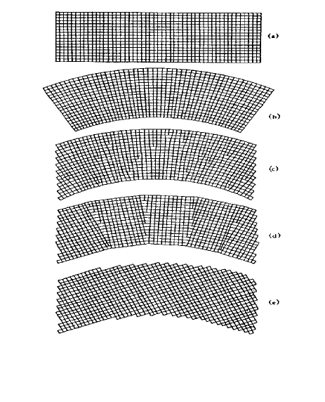
Figure 3: Five states of a single crystal. (a) Unstrained. (b) Elastically bent. (c) Plastically bent. (d) Polygonized.  (e) Recrystallized. The picture was extracted from Nabarro [95]. For the polygonized crystal, we observe large structures which are rotated against each other with a “zone” separating those blocks.  Using plainly $\operatorname{Curl\hskip 1.13791pt}p$ as the underlying defect measure would energetically penalize these configurations. Therefore it seems appropriate to use $\operatorname{inc}(\operatorname{sym}p)$ as a “weaker” defect measure which would allow for low energy configurations like that in (d).

In order to be able to describe polygonization (see Figure 3(d)), the plasticity model should energetically favour configurations in which there are blocks of many homogeneous rotations.
In this respect, the new term $\frac{1}{2}\,\mu\,L_{c}^{2}\left\lVert{\operatorname{dev}\operatorname{sym}\operatorname{Curl\hskip 1.13791pt}\operatorname{sym}p}\right\rVert^{2}=\frac{1}{2}\,\mu\,L_{c}^{2}\left\lVert{\operatorname{sym}\operatorname{Curl\hskip 1.13791pt}\operatorname{sym}p}\right\rVert^{2}$ energetically favours those configurations, which locally only rotate. The generated natural second order backstress will be of the type

$$\Sigma_{\mbox{\scriptsize curl}}=\mu\,L_{c}^{2}\,\operatorname{sym}\operatorname{Curl\hskip 1.13791pt}(\operatorname{sym}\operatorname{Curl\hskip 1.13791pt}\mbox{$\bf\varepsilon$}_{p})\,.$$

Now, looking at the invariance of the energy for which $\operatorname{sym}\operatorname{Curl\hskip 1.13791pt}(\operatorname{sym}\nabla\vartheta)=0$ versus the invariance of the backstress in the strong formulation for which $\operatorname{sym}\operatorname{Curl\hskip 1.13791pt}(\operatorname{sym}\operatorname{Curl\hskip 1.13791pt}(\operatorname{sym}\nabla\vartheta)=0$, it is clear that the invariance of the energy implies the invariance of backstress, but not vice-versa.

Remark 4.1

Note that the mapping $p\to\operatorname{dev}\operatorname{sym}\operatorname{Curl\hskip 1.13791pt}\operatorname{sym}p=\operatorname{sym}\operatorname{Curl\hskip 1.13791pt}\mbox{$\bf\varepsilon$}_{p}$ does not have any geometric meaning connected to the incompatibility of the plastic distortion $p$ like $\operatorname{Curl\hskip 1.13791pt}p$ or connected to the incompatibility of the plastic strain tensor $\mbox{$\bf\varepsilon$}_{p}=\operatorname{sym}p$ like $\operatorname{inc}(\operatorname{sym}p)$. The simpler term $\operatorname{Curl\hskip 1.13791pt}\operatorname{sym}p$ has been used by Gurtin and Anand [57] as the only energetic contribution in their irrotational gradient plasticity model.

4.3.3.  Derivation of the modified model

Now with the additional term $\mbox{W}_{\mbox{\scriptsize curl}}(\operatorname{Curl\hskip 1.13791pt}p):=\displaystyle\frac{1}{2}\,\mu\,L_{c}^{2}\,\left\lVert{\operatorname{dev}\operatorname{sym}\operatorname{Curl\hskip 1.13791pt}\mbox{$\bf\varepsilon$}_{p}}\right\rVert^{2}=\displaystyle\frac{1}{2}\,\mu\,L_{c}^{2}\,\left\lVert{\operatorname{sym}\operatorname{Curl\hskip 1.13791pt}\mbox{$\bf\varepsilon$}_{p}}\right\rVert^{2}$ in the free-energy density W, if we repeat the derivation above starting from the free-energy imbalance, we get

$$0 \leq \int_{\Omega}\Bigl{[}\langle\sigma-\mu\,L^{2}_{c}\,\operatorname{sym}\operatorname{Curl\hskip 1.13791pt}(\operatorname{sym}\operatorname{Curl\hskip 1.13791pt}\varepsilon_{p})-\mu\,\widehat{L}_{c}^{4}\,\operatorname{inc}(\operatorname{inc}\mbox{$\bf\varepsilon$}_{p}),\dot{\varepsilon}_{p}\rangle-\mu\,k_{2}\,\gamma_{p}\,\dot{\gamma}_{p}\Bigr{]}dx$$

$$\hskip 28.45274pt-\sum_{i=1}^{3}\mu\,L_{c}^{2}\int_{\partial\Omega}\langle\dot{\mbox{$\bf\varepsilon$}}_{p\,i}\times n,(\operatorname{sym}\operatorname{Curl\hskip 1.13791pt}\mbox{$\bf\varepsilon$}_{p})_{i}\rangle\,dS-\sum_{i=1}^{3}\mu\,\widehat{L}_{c}^{4}\int_{\partial\Omega}\langle\dot{\mbox{$\bf\varepsilon$}}_{p\,i}\times n,\bigl{[}\operatorname{Curl\hskip 1.13791pt}\operatorname{inc}\mbox{$\bf\varepsilon$}_{p}\bigr{]}^{T}_{i}\rangle\,dS$$

$$\hskip 28.45274pt-\sum_{i=1}^{3}\mu\,\widehat{L}_{c}^{4}\int_{\partial\Omega}\langle\bigl{[}\operatorname{Curl\hskip 1.13791pt}\dot{\mbox{$\bf\varepsilon$}}_{p}\bigr{]}^{T}_{i}\times n,\bigl{[}\operatorname{inc}\mbox{$\bf\varepsilon$}_{p}\bigr{]}_{i}\rangle\,dS$$

$$= \int_{\Omega}\Bigl{[}\langle\Sigma_{E},\dot{\varepsilon}_{p}\rangle+g\dot{\gamma}_{p}\Bigr{]}dx-\sum_{i=1}^{3}\mu\,L_{c}^{2}\int_{\partial\Omega}\langle\dot{\mbox{$\bf\varepsilon$}}_{p\,i}\times n,(\operatorname{sym}\operatorname{Curl\hskip 1.13791pt}\mbox{$\bf\varepsilon$}_{p})_{i}\rangle\,dS$$

$$\hskip 28.45274pt-\sum_{i=1}^{3}\mu\,\widehat{L}_{c}^{4}\int_{\partial\Omega}\langle\dot{\mbox{$\bf\varepsilon$}}_{p\,i}\times n,\bigl{[}\operatorname{Curl\hskip 1.13791pt}\operatorname{inc}\mbox{$\bf\varepsilon$}_{p}\bigr{]}^{T}_{i}\rangle\,dS-\sum_{i=1}^{3}\mu\,\widehat{L}_{c}^{4}\int_{\partial\Omega}\langle\bigl{[}\operatorname{Curl\hskip 1.13791pt}\dot{\mbox{$\bf\varepsilon$}}_{p}\bigr{]}^{T}_{i}\times n,\bigl{[}\operatorname{inc}\mbox{$\bf\varepsilon$}_{p}\bigr{]}_{i}\rangle\,dS$$

where

$$\Sigma_{E} := \sigma+\Sigma_{\mbox{\scriptsize curl}}+\Sigma_{\mbox{\scriptsize inc}}\,,\qquad g=-\,\mu\,k_{2}\,\gamma_{p}\,,$$

$$\Sigma_{\mbox{\scriptsize curl}} := -\,\mu\,L^{2}_{c}\,\operatorname{sym}\operatorname{Curl\hskip 1.13791pt}(\operatorname{sym}\operatorname{Curl\hskip 1.13791pt}\varepsilon_{p})\,,\quad\qquad\mbox{(second order nonlocal backstress)}$$

$$\Sigma_{\mbox{\scriptsize inc}} := -\,\mu\,\widehat{L}^{4}_{c}\,\operatorname{inc}(\operatorname{inc}\mbox{$\bf\varepsilon$}_{p})$$

$$= -\mu\,\widehat{L}^{4}_{c}\,\operatorname{Curl\hskip 1.13791pt}\Bigl{(}\Bigl{[}\operatorname{Curl\hskip 1.13791pt}\operatorname{Curl\hskip 1.13791pt}\bigl{[}\operatorname{Curl\hskip 1.13791pt}\varepsilon_{p}\bigr{]}^{T}\Bigr{]}^{T}\Bigr{)}\quad\,\mbox{(fourth order nonlocal backstress)}\,.$$

Now assuming again the simplest lower order boundary conditions

$$\varepsilon_{p}\times n|_{\partial\Omega}=0\quad\mbox{ and }\quad\bigl{[}\operatorname{Curl\hskip 1.13791pt}\varepsilon_{p}\bigr{]}^{T}\times n|_{\partial\Omega}=0$$ (4.29)

which will be clearly defined as Sobolev traces through a choice of a suitable function space for the plastic strain variable $\mbox{$\bf\varepsilon$}_{p}$, will guarantee the insulation type conditions

$$\sum_{i=1}^{3}\int_{\partial\Omega}\langle\dot{\mbox{$\bf\varepsilon$}}_{p\,i}\times n,(\operatorname{sym}\operatorname{Curl\hskip 1.13791pt}\mbox{$\bf\varepsilon$}^{p})_{i}\rangle\,dS = 0\,,$$ (4.30)

$$\sum_{i=1}^{3}\int_{\partial\Omega}\langle\dot{\mbox{$\bf\varepsilon$}}_{p\,i}\times n,\bigl{[}\operatorname{Curl\hskip 1.13791pt}\operatorname{inc}\mbox{$\bf\varepsilon$}_{p}\bigr{]}^{T}_{i}\rangle\,dS = 0\,,$$ (4.31)

$$\sum_{i=1}^{3}\int_{\partial\Omega}\langle\bigl{[}\operatorname{Curl\hskip 1.13791pt}\dot{\mbox{$\bf\varepsilon$}}_{p}\bigr{]}^{T}_{i}\times n,\bigl{[}\operatorname{inc}\mbox{$\bf\varepsilon$}_{p}\bigr{]}_{i}\rangle\,da = 0\,,$$ (4.32)

from which we obtain the global reduced dissipation inequality

$$\int_{\Omega}\bigl{[}\langle\Sigma_{E},\dot{\varepsilon}_{p}\rangle+g\,\dot{\gamma}_{p}\bigr{]}\,dx\,\geq\,0\,.$$ (4.33)

The flow law: We consider the set of admissible (elastic) generalized stresses

$$\mathcal{E}:=\{(\Sigma_{E},g)\,\,|\,\,\left\lVert{\operatorname{dev}\Sigma_{E}}\right\rVert-(\sigma_{0}-g)\leq 0,\quad g\leq 0\}\,,$$ (4.34)

whose interior Int$(\mathcal{E})$ is the elastic domain while its boundary $\partial\mathcal{E}$ is the yield surface. The constant ${\sigma}_{0}$ is the initial yield stress of the material. The flow law in its primal form reads as follows:

$$(\Sigma_{E},g)\in\partial\mathcal{D}(\dot{\mbox{$\bf\varepsilon$}}_{p},\dot{\gamma}_{p})$$ (4.35)

where

$$\mathcal{D}(q,\beta) := \sup\{\langle\Sigma_{E},q\rangle+g\beta\,\,\,|\,\,\,(\Sigma_{E},g)\in\mathcal{E}\}$$ (4.38)

$$= \sup\{\langle\Sigma_{E},q\rangle+g\,\beta\,\,\,|\,\,\,\left\lVert{\Sigma_{E}}\right\rVert\leq\sigma_{0}-g,\quad g\leq 0\}$$

$$= \left\{\begin{array}[]{ll}{\sigma}_{0}\,\left\lVert{q}\right\rVert&\mbox{ if }\left\lVert{q}\right\rVert\leq\beta,\\ \infty&\mbox{ otherwise.}\end{array}\right.$$

Here, $\partial\mathcal{D}(\dot{\Gamma}_{p})$ denotes the subdifferential of the function $\mathcal{D}$ at $\dot{\Gamma}_{p}$. That is,

$$(\Sigma_{E},g)\in\partial\mathcal{D}(\dot{\mbox{$\bf\varepsilon$}}_{p},\dot{\gamma}_{p})\quad\Leftrightarrow\quad\langle\Sigma_{E},q-\dot{\mbox{$\bf\varepsilon$}}_{p}\rangle+g(\beta-\dot{\gamma}_{p})\leq\mathcal{D}(q,\beta)-\mathcal{D}(\dot{\mbox{$\bf\varepsilon$}}_{p},\dot{\gamma}_{p})\quad\forall\,(q,\beta)\,.$$ (4.39)

Now using convex analysis, we get

$$(\Sigma_{E},g)\in\partial\mathcal{D}(\dot{\mbox{$\bf\varepsilon$}}_{p},\dot{\gamma}_{p})\quad\Leftrightarrow\quad(\dot{\mbox{$\bf\varepsilon$}}_{p},\dot{\gamma_{p}})\in\partial I_{\mathcal{E}}(\Sigma_{E},g)=N_{\mathcal{E}}(\Sigma_{E},g)\,,$$ (4.40)

where $I_{\mathcal{E}}$ is the indicator function of the set $\mathcal{E}$ of admissible generalized stresses and $N_{\mathcal{E}}(\Sigma_{E},g)$ is the normal cone of the set $\mathcal{E}$ at $(\Sigma_{E},g)$.
The condition (4.40)₂ is called the dual form of the flow law, which in the case of smoothness of the yield surface $\partial\mathcal{E}$ at $(\Sigma_{E},g)$ gives for some scalar parameter $\lambda\geq 0$

$$\dot{\mbox{$\bf\varepsilon$}}_{p}=\lambda\,\frac{\operatorname{dev}\Sigma_{E}}{\left\lVert{\operatorname{dev}\Sigma_{E}}\right\rVert}\quad\mbox{ and }\quad\dot{\gamma}_{p}=\lambda=\left\lVert{\dot{\mbox{$\bf\varepsilon$}}_{p}}\right\rVert$$ (4.41)

together with the Karush-Kuhn-Tucker complementary conditions:

$$\lambda\geq 0\,,\quad\phi(\Sigma_{E},g)\leq 0\quad\mbox{ and }\quad\lambda\,\phi(\Sigma_{\mbox{\scriptsize E}},g)=0\,.$$

Note that with this choice, the global dissipation inequality (4.33) is satisfied.

4.3.4.  Mathematical strong formulation of the model

Taking into account the free energy density $W$ in (4.8) together with the additional term in (4.16) and the constraint $\left\lVert{q}\right\rVert\leq\beta$ in the definition of the dissipation function $\mathcal{D}$ in (4.38), the model is strongly formulated as follows: find

• the displacement $u\in\mbox{$\mathsf{H}$}^{1}(0,T;\mbox{$\mathsf{H}$}^{1}_{0}(\Omega,{\Gamma},\mathbb{R}^{3}))$ ,

• the infinitesimal plastic strain $\mbox{$\bf\varepsilon$}_{p}\in\mbox{$\mathsf{H}$}^{1}(0,T;L^{2}(\Omega,\operatorname{\mathfrak{sl}}(3)\cap\mbox{Sym}(3)))$ with

  $$\operatorname{sym}\operatorname{Curl\hskip 1.13791pt}\mbox{$\bf\varepsilon$}_{p} \in \mbox{$\mathsf{H}$}^{1}(0,T;L^{2}(\Omega,\mbox{Sym}(3)\cap\operatorname{\mathfrak{sl}}(3)));$$

  $$\operatorname{inc}\mbox{$\bf\varepsilon$}_{p}=\operatorname{Curl\hskip 1.13791pt}[(\operatorname{Curl\hskip 1.13791pt}\mbox{$\bf\varepsilon$}_{p})^{T}] \in \mbox{$\mathsf{H}$}^{1}(0,T;L^{2}(\Omega,\mbox{$\mathbb{R}$}^{3\times 3}));$$

  $$\operatorname{inc}\operatorname{inc}\mbox{$\bf\varepsilon$}_{p}=\operatorname{Curl\hskip 1.13791pt}\Bigl{(}\bigl{[}\operatorname{Curl\hskip 1.13791pt}\operatorname{Curl\hskip 1.13791pt}[(\operatorname{Curl\hskip 1.13791pt}\mbox{$\bf\varepsilon$}_{p})^{T}]\bigr{]}^{T}\Bigr{)} \in \mbox{$\mathsf{H}$}^{1}(0,T;L^{2}(\Omega,\mbox{$\mathbb{R}$}^{3\times 3}))\,,$$

• The internal isotropic hardening variable $\gamma_{p}\in\mbox{$\mathsf{H}$}^{1}(0,T;L^{2}(\Omega))$ ,

such that the content of Table 9 holds.

Additive split of strain:	$\operatorname{sym}\nabla u=\mbox{$\bf\varepsilon$}_{e}+\mbox{$\bf\varepsilon$}_{p}$
Equilibrium:	$\mbox{Div}\,\sigma+f=0$ with $\sigma=\mathbb{C}_{\mbox{\scriptsize{iso}}}\mbox{$\bf\varepsilon$}_{e}$
Free energy:	$\displaystyle\frac{1}{2}\,\langle\mathbb{C}_{\mbox{\scriptsize{iso}}}\mbox{$\bf\varepsilon$}_{e},\mbox{$\bf\varepsilon$}_{e}\rangle+\frac{1}{2}\,\mu\,k_{2}\,|\gamma_{p}|^{2}+\,\,\frac{1}{2}\,\mu\,L^{2}_{c}\left\lVert{\operatorname{sym}\operatorname{Curl\hskip 1.13791pt}\mbox{$\bf\varepsilon$}_{p}}\right\rVert^{2}+\,\frac{1}{2}\,\mu\,\widehat{L}^{4}_{c}\left\lVert{\operatorname{inc}\mbox{$\bf\varepsilon$}_{p}}\right\rVert^{2}$
Yield condition:	$\phi(\Sigma_{E},g):=\left\lVert{\operatorname{dev}\Sigma_{E}}\right\rVert^{2}-({\sigma}_{0}-g)\leq 0$ where  $g:=-\mu\,k_{2}\gamma_{p}$
	$\begin{array}[]{lcl}\Sigma_{E}&:=&\sigma+\Sigma_{\mbox{\scriptsize curl}}+\Sigma_{\mbox{\scriptsize inc}}\,,\\ \Sigma_{\mbox{\scriptsize curl}}&:=&-\,\mu\,L^{2}_{c}\,\operatorname{sym}\operatorname{Curl\hskip 1.13791pt}(\operatorname{sym}\operatorname{Curl\hskip 1.13791pt}\varepsilon_{p})\\ \Sigma_{\mbox{\scriptsize inc}}&:=&-\mu\,\widehat{L}^{4}_{c}\,\operatorname{inc}\operatorname{inc}\mbox{$\bf\varepsilon$}_{p}\,=\,\operatorname{Curl\hskip 1.13791pt}\bigl{[}\operatorname{Curl\hskip 1.13791pt}\operatorname{Curl\hskip 1.13791pt}[\operatorname{Curl\hskip 1.13791pt}\mbox{$\bf\varepsilon$}_{p}]^{T}\bigr{]}^{T}\end{array}$
Dissipation inequality:	$\displaystyle\int_{\Omega}\bigl{[}\langle\Sigma_{E},\dot{\mbox{$\bf\varepsilon$}}_{p}\rangle+g\,\dot{\gamma}_{p}\rangle\bigr{]}\,dx\geq 0$
Dissipation function:	$\mathcal{D}(\dot{\mbox{$\bf\varepsilon$}}_{p},\dot{\gamma}_{p}):=\left\{\begin{array}[]{ll}{\sigma}_{0}\,\left\lVert{\dot{\mbox{$\bf\varepsilon$}}_{p}}\right\rVert&\mbox{ if }\left\lVert{\dot{\mbox{$\bf\varepsilon$}}_{p}}\right\rVert\leq\dot{\gamma}_{p},\\ \infty&\mbox{ otherwise}\end{array}\right.$
Flow law in primal form:	$(\Sigma_{E},g)\in\partial\mathcal{D}(\dot{\mbox{$\bf\varepsilon$}}_{p},\dot{\gamma}_{p})$
Flow law in dual form:	$\dot{\mbox{$\bf\varepsilon$}}_{p}=\lambda\,\displaystyle\frac{\operatorname{dev}\Sigma_{E}}{\left\lVert{\operatorname{dev}\Sigma_{E}}\right\rVert},\quad\quad\dot{\gamma}_{p}=\lambda=\left\lVert{\dot{\mbox{$\bf\varepsilon$}}_{p}}\right\rVert$
KKT conditions:	$\lambda\geq 0$,  $\phi(\Sigma_{E},g)\leq 0$,  $\lambda\,\phi(\Sigma_{E},g)=0$
Boundary conditions for $\mbox{$\bf\varepsilon$}_{p}$:	$\mbox{$\bf\varepsilon$}_{p}\times n|_{\partial\Omega}=0\,,\quad(\operatorname{Curl\hskip 1.13791pt}\mbox{$\bf\varepsilon$}_{p})^{T}\times n|_{\partial\Omega}=0$

Table 9: The new regularized irrotational model with isotropic hardening and Kröner’s incompatibility tensor. Also in this case, the boundary condition on $\mbox{$\bf\varepsilon$}_{p}$ necessitates at least $\mbox{$\bf\varepsilon$}_{p},\,\,(\operatorname{Curl\hskip 1.13791pt}\mbox{$\bf\varepsilon$}_{p})^{T}\in\mbox{H}(\mbox{Curl};\,\Omega,\,\mbox{$\mathbb{R}$}^{3\times 3})$. The model is micro-random i.e., invariant w.r.t. $p\to p+A(x)$, $A(x)\in\operatorname{\mathfrak{so}}(3)$ and invariant under infinitesimal conformal mappings $p\to p+\nabla\phi_{c}$ with $\operatorname{dev}\operatorname{sym}\nabla\phi_{c}=0$.

4.3.5.  Weak formulation of the model

To obtain the weak formulation of the model, we consider the equilibrium in its weak formulation. That is, for every $v\in\mbox{$\mathsf{H}$}^{1}_{0}(\Omega,\mathbb{R}^{3})$ we have

$$\int_{\Omega}\langle\mathbb{C}_{\mbox{\scriptsize{iso}}}(\operatorname{sym}\nabla u-\mbox{$\bf\varepsilon$}_{p}),\mbox{sym}(\nabla v-\nabla\dot{u})\rangle dx=\int_{\Omega}f(v-\dot{u})dx\,.$$ (4.42)

On the other hand, for every $q\in C^{\infty}(\overline{\Omega},\operatorname{\mathfrak{sl}}(3)\cap\mbox{Sym}(3))$ such that

$$q\times n|_{\partial\Omega}=0\quad\mbox{ and }\quad(\operatorname{Curl\hskip 1.13791pt}q)^{T}\times n|_{\partial\Omega}=0\,$$

and for every $\beta\in L^{2}(\Omega)$, integrate (4.39) over $\Omega$ using the pair of functions $(q,\beta)$ and get

$$\int_{\Omega}\mathcal{D}(q,\beta)\,dx \geq \int_{\Omega}\mathcal{D}(\dot{\mbox{$\bf\varepsilon$}}_{p},\dot{\gamma}_{p})\,dx+\int_{\Omega}\bigl{[}\langle\sigma+\Sigma_{\mbox{\scriptsize curl}}+\Sigma_{\mbox{\scriptsize inc}},q-\dot{\mbox{$\bf\varepsilon$}}_{p}\rangle+g\,(\beta-\dot{\gamma}_{p})\bigr{]}\,dx$$

$$= \int_{\Omega}\bigl{[}\langle\sigma-\mu\,L^{2}_{c}\,\operatorname{sym}\operatorname{Curl\hskip 1.13791pt}(\operatorname{sym}\operatorname{Curl\hskip 1.13791pt}\varepsilon_{p})-\mu\,\widehat{L}^{4}_{c}\,\operatorname{inc}\operatorname{inc}\mbox{$\bf\varepsilon$}_{p},q-\dot{\mbox{$\bf\varepsilon$}}_{p}\rangle$$

$$\hskip 56.9055pt-\mu\,k_{2}\,\gamma_{p}\,(\beta-\dot{\gamma}_{p})\bigr{]}\,dx\,.$$

Now integrating by parts the two terms $\langle\operatorname{sym}\operatorname{Curl\hskip 1.13791pt}(\operatorname{sym}\operatorname{Curl\hskip 1.13791pt}\varepsilon_{p}),q-\dot{\mbox{$\bf\varepsilon$}}_{p}\rangle$ once and $\langle\operatorname{inc}\operatorname{inc}\mbox{$\bf\varepsilon$}_{p},q-\dot{\mbox{$\bf\varepsilon$}}_{p}\rangle$ twice, using the boundary conditions

$$(q-\dot{\mbox{$\bf\varepsilon$}}_{p})\times n|_{\partial\Omega}=0\quad\mbox{ and }\quad(\operatorname{Curl\hskip 1.13791pt}(q-\dot{\mbox{$\bf\varepsilon$}}_{p}))^{T}\times n|_{\partial\Omega}=0\,$$

we get from (4.3.5) that

$$\int_{\Omega}\mathcal{D}(q,\beta)\,dx \geq \int_{\Omega}\mathcal{D}(\dot{\mbox{$\bf\varepsilon$}}_{p},\dot{\gamma}_{p})\,dx+\int_{\Omega}\langle\mathbb{C}_{\mbox{\scriptsize{iso}}}(\operatorname{sym}\nabla u-\mbox{$\bf\varepsilon$}_{p}),\,q-\dot{\mbox{$\bf\varepsilon$}}_{p}\rangle\,dx$$ (4.44)

$$-\mu\,k_{2}\int_{\Omega}\gamma_{p}(\beta-\dot{\gamma}_{p})\,dx\,-\,\mu\,L^{2}_{c}\int_{\Omega}\langle\operatorname{sym}\operatorname{Curl\hskip 1.13791pt}\mbox{$\bf\varepsilon$}_{p},\,\operatorname{sym}\operatorname{Curl\hskip 1.13791pt}(q-\dot{\mbox{$\bf\varepsilon$}}_{p})\rangle\,dx$$

$$-\,\mu\,\widehat{L}^{4}_{c}\int_{\Omega}\langle\operatorname{inc}\mbox{$\bf\varepsilon$}_{p},\,\operatorname{inc}(q-\dot{\mbox{$\bf\varepsilon$}}_{p})\rangle\,dx\,.$$

Adding (4.44) to the weak formulation of the equilibrium in (4.42), we get the weak formulation of our model of gradient plasticity with isotropic hardening and Kröner’s incompatibility tensor

$$\hskip-28.45274pt\int_{\Omega}\Bigl{[}\langle\mathbb{C}_{\mbox{\scriptsize{iso}}}(\operatorname{sym}\nabla u-\mbox{$\bf\varepsilon$}_{p}),(\operatorname{sym}\nabla v-q)-(\operatorname{sym}\nabla\dot{u}-\dot{\mbox{$\bf\varepsilon$}}_{p})\rangle+\mu\,k_{2}\gamma_{p}(\beta-\dot{\gamma}_{p})$$

$$\quad+\,\mu\,L^{2}_{c}\,\langle\operatorname{sym}\operatorname{Curl\hskip 1.13791pt}\mbox{$\bf\varepsilon$}_{p},\,\operatorname{sym}\operatorname{Curl\hskip 1.13791pt}(q-\dot{\mbox{$\bf\varepsilon$}}_{p})\rangle+\,\mu\,\widehat{L}^{4}_{c}\langle\operatorname{inc}\mbox{$\bf\varepsilon$}_{p},\,\operatorname{inc}(q-\dot{\mbox{$\bf\varepsilon$}}_{p})\rangle\Bigr{]}\,dx$$

$$\quad+\,\int_{\Omega}\mathcal{D}(q,\beta)\,dx-\int_{\Omega}\mathcal{D}(\dot{\mbox{$\bf\varepsilon$}}_{p},\dot{\gamma}_{p})\,dx\,\geq\,\int_{\Omega}f(v-\dot{u})\,dx\,.$$ (4.45)

That is,

$$\mbox{\boldmath{$a$}}(w,z-\dot{w})+j(z)-j(\dot{w})\geq\langle\ l,z-\dot{w}\rangle\,,$$ (4.46)

where

$$\mbox{\boldmath{$a$}}(w,z) := \int_{\Omega}\Bigl{[}\langle\mathbb{C}_{\mbox{\scriptsize{iso}}}(\operatorname{sym}(\nabla u-p)),\operatorname{sym}\nabla v-q\rangle+\mu\,k_{2}\,\gamma_{p}\,\beta+$$ (4.47)

$$\hskip 56.9055pt+\,\,\mu\,L_{c}^{2}\,\langle\operatorname{sym}\operatorname{Curl\hskip 1.13791pt}\mbox{$\bf\varepsilon$}_{p},\,\operatorname{sym}\operatorname{Curl\hskip 1.13791pt}q\rangle+\,\mu\,\widehat{L}_{c}^{4}\langle\operatorname{inc}\mbox{$\bf\varepsilon$}_{p},\,\operatorname{inc}q\rangle\Bigr{]}dx\,,$$

$$j(z) := \int_{\Omega}\mathcal{D}(q,\beta)\,dx\,,$$ (4.48)

$$\langle l,z\rangle := \int_{\Omega}fv\,dx\,,$$ (4.49)

for $w=(u,\mbox{$\bf\varepsilon$}_{p},\gamma_{p})$ and $z=(v,q,\beta)$ .

4.3.6.  Existence result for the weak formulation

We prove the existence result for the weak formulation (4.3.5) by closely following the approach by now classical, which uses the abstract machinery developed by Han and Reddy in [62] for mathematical problems in geometrically linear classical plasticity and used for instance in [35, 123, 101, 38, 42] for models of gradient plasticity. Precisely, we will need the following Theorem.

Theorem 4.2

([62, Theorem 6.19])
Let $\mathsf{Z}$ be a Hilbert space and let $\mathsf{W}$ be a nonempty closed convex cone in $\mathsf{Z}$. Consider the following problem: find $w\in\mbox{$\mathsf{H}$}^{1}([0,T];\mbox{$\mathsf{Z}$})$ with $w(0)=0$ such that for almost every $t\in[0,T]$, $\dot{w}(t)\in\mbox{$\mathsf{W}$}$ and

$$\mbox{\boldmath{$a$}}(w,z-\dot{w})+j(z)-j(\dot{w})\geq\langle\ell,z-\dot{w}\rangle\mbox{ for every }z\in\mbox{$\mathsf{W}$}\,.$$ (4.50)

Assume that the following hold:

• the bilinear form $a$ is symmetric, continuous on $\mathsf{Z}$ and coercive on $\mathsf{W}$, i.e., there exist $C>0$ and $\alpha>0$ such that

  $$\mbox{\boldmath{$a$}}(w,z)\leq C\,\left\lVert{w}\right\rVert_{Z}\,\left\lVert{z}\right\rVert_{Z}\qquad\forall w,\,z\in\mbox{$\mathsf{Z}$}\quad\mbox{ and }\quad\mbox{\boldmath{$a$}}(z,z)\geq\alpha\,\left\lVert{z}\right\rVert^{2}_{Z}\qquad\forall z\in\mbox{$\mathsf{W}$}\,;$$ (4.51)

• $\ell\in\mbox{$\mathsf{H}$}^{1}([0,T];\mbox{$\mathsf{Z}$}^{\prime})$ with $\ell(0)=0$.

• the functional $j$ is non-negative, convex, lower continuous and positively $1$-homogeneous $\mathsf{W}$, i.e., $j(sz)=|s|\,j(z)\quad\forall s\in\mathbb{R}\,,\quad\forall z\in\mbox{$\mathsf{Z}$}\,.$

Then the problem (4.50) has a solution $w\in\mbox{$\mathsf{H}$}^{1}([0,T];\mbox{$\mathsf{Z}$})$.

Therefore, the problem is then reduced to finding a suitable Hilbert space $\mathsf{Z}$ and its subset $\mathsf{W}$ such that the bilinear form $\mbox{\boldmath{$a$}}(\cdot,\cdot)$ and the functionals $j$ and $\ell$ satisfies the assumptions of Theorem 4.2. The choices of function spaces for the displacement variable $u$ and the isotropic hardening variable $\gamma_{p}$ are straightforward as

$$u\in\mbox{$\mathsf{H}$}^{1}_{0}(\Omega,\mathbb{R}^{3})\quad\mbox{ and }\quad\gamma_{p}\in\mbox{$\mathsf{L}$}^{2}(\Omega)\,.$$

For the plastic strain variable $\mbox{$\bf\varepsilon$}_{p}$, we first need to introduce the space

$$\hskip-11.38092pt\mbox{$\mathsf{H}$}_{\mbox{\scriptsize inc }}(\operatorname{Curl\hskip 1.13791pt},\,\Omega;\operatorname{\mathfrak{sl}}(3)\cap\mbox{Sym}(3)) := \{q\in\mbox{$\mathsf{L}$}^{2}(\Omega,\,\operatorname{\mathfrak{sl}}(3)\cap\mbox{Sym}(3)\,\,|\,\,(\operatorname{Curl\hskip 1.13791pt}q)^{T}\in\mbox{$\mathsf{H}$}(\operatorname{Curl\hskip 1.13791pt},\,\Omega;\mathbb{R}^{3\times 3})\}$$ (4.52)

$$:= \{q\in\mbox{$\mathsf{H}$}(\Omega,\,\operatorname{\mathfrak{sl}}(3)\cap\mbox{Sym}(3)\,\,|\,\,\operatorname{inc}q\in\mbox{$\mathsf{L}$}^{2}(\operatorname{Curl\hskip 1.13791pt},\,\Omega;\mathbb{R}^{3\times 3})\}$$

equipped with the norm

$$\left\lVert{q}\right\rVert^{2}_{\mbox{\scriptsize inc}} := \left\lVert{q}\right\rVert^{2}_{L^{2}(\Omega)}+\left\lVert{(\operatorname{Curl\hskip 1.13791pt}q)^{T}}\right\rVert^{2}_{\mbox{\scriptsize H}(\mbox{\scriptsize Curl};\Omega)}\,=\,\left\lVert{q}\right\rVert^{2}_{L^{2}}+\left\lVert{(\operatorname{Curl\hskip 1.13791pt}q)^{T}}\right\rVert^{2}_{L^{2}}+\left\lVert{\operatorname{Curl\hskip 1.13791pt}(\operatorname{Curl\hskip 1.13791pt}q)^{T}}\right\rVert^{2}_{L^{2}}$$ (4.53)

$$= \left\lVert{q}\right\rVert^{2}_{\mbox{\scriptsize H}(\mbox{\scriptsize Curl};\Omega)}+\left\lVert{\operatorname{inc}q}\right\rVert^{2}_{L^{2}(\Omega)}\,.$$

Let us mention that spaces of functions involving the inc-operator were already used in the literature and we refer the interested reader for instance to the papers [10, 11].

We also consider the closure $\mbox{$\mathsf{H}$}_{\mbox{\scriptsize sym, inc }}(\operatorname{Curl\hskip 1.13791pt},\,\Omega,\partial\Omega;\operatorname{\mathfrak{sl}}(3)\cap\mbox{Sym}(3))$ of the linear subspace

$$\Bigl{\{}q\in C^{\infty}(\overline{\Omega},\mbox{Sym}(3))\,\,|\,\,\operatorname{tr}{q}=0,\,\,q\times\,n|_{\partial\Omega}=0\mbox{ and }(\operatorname{Curl\hskip 1.13791pt}q)^{T}\times n|_{\partial\Omega}=0\Bigr{\}}$$

in the norm

$$\left\lVert{q}\right\rVert_{\mbox{\scriptsize symcurl,\,inc}}^{2}:=\left\lVert{q}\right\rVert^{2}_{L^{2}}+\left\lVert{\operatorname{sym}\mbox{Curl\,}q}\right\rVert^{2}_{L^{2}}+\left\lVert{\operatorname{inc}q}\right\rVert^{2}_{L^{2}}\,.$$ (4.54)

Motivated by the well-posedness question for models of infinitesimal gradient plasticity (specially for models dictated by invariance under infinitesimal rotations) [116, 117, 38, 115, 101], infinitesimal Cosserat elasticity [106, 66, 97], infinitesimal Cosserat elasto-plasticity [100, 109, 27, 102] and infinitesimal relaxed micromorphic [105, 108, 98], Bauer et al. [21, 22] (see also Neff et al. [111, 112, 113, 114]) derived a new inequality extending Korn’s first inequality to incompatible tensor fields, namely there exists a constant $C(\Omega)>0$ such that

$$\forall\,X\in\mbox{$\mathsf{H}$}(\operatorname{Curl\hskip 1.13791pt};\,\Omega,\,\mbox{$\mathbb{R}$}^{3\times 3}),\quad X\times\,n|_{\partial\Omega}=0:$$ (4.55)

$$\|X\|_{L^{2}(\Omega)}\leq C(\Omega)\,\Big{(}\left\lVert{\operatorname{sym}X}\right\rVert_{L^{2}(\Omega)}+\left\lVert{\operatorname{Curl\hskip 1.13791pt}X}\right\rVert_{L^{2}(\Omega)}\Big{)}\,.$$

Now, if we apply the incompatible Korn’s type inequality to $X=(\operatorname{Curl\hskip 1.13791pt}q)^{T}$ for $q\in C^{\infty}(\overline{\Omega},\mbox{Sym}(3))$ with $(\operatorname{Curl\hskip 1.13791pt}q)^{T}\times n|_{\partial\Omega}=0$, we get

$$\left\lVert{\operatorname{Curl\hskip 1.13791pt}q}\right\rVert_{L^{2}(\Omega)} = \left\lVert{(\operatorname{Curl\hskip 1.13791pt}q)^{T}}\right\rVert_{L^{2}(\Omega)}$$ (4.56)

$$\leq C(\Omega)\Bigl{(}\left\lVert{\operatorname{sym}\Bigl{(}(\operatorname{Curl\hskip 1.13791pt}q)^{T}\Bigr{)}}\right\rVert_{L^{2}(\Omega)}+\left\lVert{\operatorname{Curl\hskip 1.13791pt}[(\operatorname{Curl\hskip 1.13791pt}\mbox{$\bf\varepsilon$}_{p})^{T}]}\right\rVert_{L^{2}(\Omega)}\Bigr{)}$$

$$= C(\Omega)\Bigl{(}\left\lVert{\operatorname{sym}\operatorname{Curl\hskip 1.13791pt}q}\right\rVert_{L^{2}(\Omega)}+\left\lVert{\operatorname{inc}q}\right\rVert_{L^{2}(\Omega)}\Bigr{)}\,,$$

then we have the decisive identity

$$\hskip-42.67912pt\mbox{$\mathsf{H}$}_{\mbox{\scriptsize sym, inc }}(\operatorname{Curl\hskip 1.13791pt},\,\Omega,\partial\Omega;\operatorname{\mathfrak{sl}}(3)\cap\mbox{Sym}(3))$$

$$\hskip 14.22636pt\equiv \bigl{\{}q\in\mbox{$\mathsf{H}$}_{0}(\operatorname{Curl\hskip 1.13791pt},\,\Omega,\partial\Omega;\operatorname{\mathfrak{sl}}(3)\cap\mbox{Sym}(3)),\quad(\operatorname{Curl\hskip 1.13791pt}q)^{T}\in\mbox{$\mathsf{H}$}_{0}(\operatorname{Curl\hskip 1.13791pt},\,\Omega,\partial\Omega;\mathbb{R}^{3\times 3})\bigr{\}}$$

$$\hskip 14.22636pt= \bigl{\{}q,\,(\operatorname{Curl\hskip 1.13791pt}q)^{T}\in\mbox{$\mathsf{H}$}(\operatorname{Curl\hskip 1.13791pt},\,\Omega,\mathbb{R}^{3\times 3}),\quad\operatorname{tr}q=0\mbox{ a.e. in }\Omega,\quad q\times n|_{\partial\Omega}=(\operatorname{Curl\hskip 1.13791pt}q)^{T}\times n|_{\partial\Omega}=0\bigr{\}}$$

with the norms $\left\lVert{\cdot}\right\rVert_{\mbox{\scriptsize inc}}$ and $\left\lVert{\cdot}\right\rVert_{\mbox{\scriptsize symcurl,\,inc}}$ being equivalent. Now, we set

$$\mbox{V}: = \mbox{H}^{1}_{0}(\Omega;\,\mathbb{R}^{3})\,,$$ (4.58)

$$\mbox{Q}: = \bigl{\{}q\in\mbox{$\mathsf{H}$}_{\mbox{\scriptsize inc }}(\operatorname{Curl\hskip 1.13791pt},\,\Omega;\operatorname{\mathfrak{sl}}(3)\cap\mbox{Sym}(3))\,\,|\,\,q\times n|_{\partial\Omega}=0\mbox{ and }(\operatorname{Curl\hskip 1.13791pt}q)^{T}\times n|_{\partial\Omega}=0\bigr{\}}\,,$$ (4.59)

$$\Lambda: = \mbox{L}^{2}(\Omega)\,,$$ (4.60)

$$\mbox{Z}: = \mbox{V}\times\mbox{Q}\times\Lambda\,,$$ (4.61)

$$\mbox{W}: = \{z=(v,q,\beta)\in\mbox{Z}\,\,|\,\,\left\lVert{q}\right\rVert\leq\beta\}\,,$$ (4.62)

equipped with the norms

$$\left\lVert{v}\right\rVert_{V}:=\left\lVert{\nabla v}\right\rVert_{L^{2}(\Omega)},\quad\qquad\left\lVert{q}\right\rVert_{Q}:=\left\lVert{q}\right\rVert_{\mbox{\scriptsize inc}}\,\,,\quad\qquad\left\lVert{\beta}\right\rVert_{\Lambda}=\left\lVert{\beta}\right\rVert_{L^{2}(\Omega)}\,,$$

$$\left\lVert{z}\right\rVert^{2}_{Z}:=\left\lVert{v}\right\rVert^{2}_{V}+\left\lVert{q}\right\rVert^{2}_{Q}+\left\lVert{\beta}\right\rVert^{2}_{\Lambda}\quad\mbox{ for }z=(v,q,\beta)\in Z\,.$$ (4.63)

Let us prove the coercivity of the bilinear form $\mbox{\boldmath{$a$}}(\cdot,\cdot)$ on the closed convex set $\mathsf{W}$, where the constraint $\left\lVert{q}\right\rVert\leq\beta$ in $\mathsf{W}$ plays a crucial role. Let therefore $z=(v,q,\beta)\in\mbox{$\mathsf{W}$}$. Then,

$$\mbox{\boldmath{$a$}}(z,z) \geq m_{0}\left\lVert{\operatorname{sym}(\nabla v)-q}\right\rVert^{2}_{2}+\mu\,k_{2}\left\lVert{\beta}\right\rVert^{2}_{L^{2}}+\mu\,L^{2}_{c}\,\left\lVert{\operatorname{sym}\operatorname{Curl\hskip 1.13791pt}q}\right\rVert^{2}+\mu\,\widehat{L}_{c}^{4}\left\lVert{\operatorname{inc}q}\right\rVert_{L^{2}}^{2}$$

($$m_{0}>0$$ is from (2.3))

$$= m_{0}\left[\left\lVert{\operatorname{sym}(\nabla v)}\right\rVert^{2}_{2}+\left\lVert{q}\right\rVert^{2}_{L^{2}}-2\langle\operatorname{sym}(\nabla v),p\rangle\right]+\mu\,k\left\lVert{\beta}\right\rVert_{L^{2}}^{2}$$

$$\hskip 85.35826pt+\mu\,L^{2}_{c}\,\left\lVert{\operatorname{sym}\operatorname{Curl\hskip 1.13791pt}q}\right\rVert^{2}+\mu\,\widehat{L}_{c}^{4}\,\left\lVert{\operatorname{inc}q)}\right\rVert_{L^{2}}^{2}$$

$$\geq m_{0}\left[\left\lVert{\operatorname{sym}(\nabla v)}\right\rVert^{2}_{L^{2}}+\left\lVert{q}\right\rVert^{2}_{L^{2}}-\theta\left\lVert{\operatorname{sym}(\nabla v)}\right\rVert_{L^{2}}^{2}-\frac{1}{\theta}\left\lVert{q}\right\rVert_{L^{2}}^{2}\right]+\frac{1}{2}\mu\,k_{2}\left\lVert{\beta}\right\rVert_{2}^{2}$$

$$+\frac{1}{2}\mu\,k_{2}\left\lVert{q}\right\rVert_{L^{2}}^{2}+\mu\,L^{2}_{c}\,\left\lVert{\operatorname{sym}\operatorname{Curl\hskip 1.13791pt}q}\right\rVert^{2}_{L^{2}}+\mu\,\widehat{L}_{c}^{4}\left\lVert{\operatorname{inc}q}\right\rVert_{L^{2}}^{2}$$

$$\mbox{ (using Young's inequality and }\left\lVert{q}\right\rVert\leq\beta\mbox{ from }W)$$

$$= m_{0}(1-\theta)\left\lVert{\operatorname{sym}(\nabla v)}\right\rVert^{2}_{2}+\left[m_{0}(1-\frac{1}{\theta})+\frac{1}{2}\mu\,k_{2}\right]\left\lVert{q}\right\rVert_{2}^{2}+\frac{1}{2}\mu\,k_{2}\left\lVert{\beta}\right\rVert_{2}^{2}$$

$$+\mu\,L_{c}^{2}\left\lVert{\operatorname{sym}\operatorname{Curl\hskip 1.13791pt}q}\right\rVert^{2}_{L^{2}}+\mu\,\widehat{L}_{c}^{4}\left\lVert{\operatorname{inc}q}\right\rVert_{L^{2}}^{2}\,.$$

So, choosing $\theta$ such that $\displaystyle\frac{2\,m_{0}}{2\,m_{0}+\mu\,k_{2}}\leq\theta<1,$ and using the classical Korn’s first inequality, there exists some positive constant $K(m_{0},\,\mu\,,k_{2}\,,\Omega)>0$ such that

$$\mbox{\boldmath{$a$}}(z,z) \geq K\left[\left\lVert{v}\right\rVert_{V}^{2}+\left\lVert{q}\right\rVert^{2}_{L^{2}}+\left\lVert{\beta}\right\rVert_{\Lambda}^{2}+\mu\,L^{2}_{c}\,\left\lVert{\operatorname{sym}\operatorname{Curl\hskip 1.13791pt}q}\right\rVert^{2}_{L^{2}}+\mu\,\widehat{L}_{c}^{4}\left\lVert{\operatorname{inc}q}\right\rVert_{L^{2}}^{2}\right]$$

$$\geq C\left[\left\lVert{v}\right\rVert_{V}^{2}+\left\lVert{q}\right\rVert^{2}_{Q}+\left\lVert{\beta}\right\rVert_{\Lambda}^{2}\right]\,=\,C\left\lVert{z}\right\rVert^{2}_{Z}\quad\forall z=(v,q,\beta)\in W\,,$$

where $C=C(m_{0},\,\mu\,,k_{2}\,,\Omega,L_{c},\widehat{L}_{c})>0$. For the second inequality in (4.3.6), we used the inequality (4.56) obtained as a consequence of Korn’s type inequality for incompatible tensor fields in Neff et al. [111, 112, 113, 114] .   $\blacksquare$

So, assuming that the body is initially unloaded and undeformed, which corresponds to assuming that $f(x,0)=0$ for almost all $x\in\Omega$ with homogeneous initial conditions, we obtained the following existence result for the weak formulation (4.3.5) of our model.

Theorem 4.3

Under the choices of the Hilbert space $\mathsf{Z}$ and the closed convex cone $\mathsf{W}$ in (4.58)-(4.62) with the norms in (4.63) and the functionals $a$, $j$ and $\ell$ in (4.47)-(4.49), the weak formulation (4.3.5) when written as the variational inequality of the second kind (4.50) has a solution $w=(u,\mbox{$\bf\varepsilon$}_{p},\gamma_{p})$ in $\mbox{$\mathsf{H}$}^{1}([0,T];\mbox{$\mathsf{Z}$})$ with $\dot{w}\in\mbox{$\mathsf{L}$}^{2}([0,T];\mbox{$\mathsf{W}$})$.

Remark 4.2

Uniqueness of the strong solution is obtained as in [41] provided the following further assumptions are satisfied:

$$\operatorname{sym}\operatorname{Curl\hskip 1.13791pt}\bigl{(}\operatorname{sym}\operatorname{Curl\hskip 1.13791pt}\mbox{$\bf\varepsilon$}_{p}\bigr{)} \in \mbox{$\mathsf{L}$}^{2}(\Omega,\mbox{Sym}(3)\cap\operatorname{\mathfrak{sl}}(3))\,$$ (4.65)

$$\operatorname{Curl\hskip 1.13791pt}\Bigl{(}[\operatorname{Curl\hskip 1.13791pt}\operatorname{Curl\hskip 1.13791pt}[\operatorname{Curl\hskip 1.13791pt}\mbox{$\bf\varepsilon$}_{p}]^{T}]^{T}\Bigr{)} \in \mbox{$\mathsf{L}$}^{2}(\Omega,\mathbb{R}^{3\times 3})\,.$$

5.  Discussion

It remains a difficult task to reconcile mathematical and physical requirements. Indeed, the incorporation of Kröner’s incompatibility tensor $\operatorname{inc}\mbox{$\bf\varepsilon$}_{p}$ is physically transparent and the novel model is micro-random and gauge-invariant. Micro-randomness being useful for polycrystals and gauge-invariance being a generally physically necessary requirement. However, using integration by parts in order to arrive at a global reduced dissipation inequality, the following lowest order boundary conditions

$$\mbox{$\bf\varepsilon$}_{p}\times n|_{\partial\Omega}=0\quad\mbox{ and }\quad(\operatorname{Curl\hskip 1.13791pt}\mbox{$\bf\varepsilon$}_{p})^{T}\times n|_{\partial\Omega}=0$$ (5.1)

impose themselves.

From a mathematical point of view these expressions are, however, not well-defined as boundary traces through a control of the given free-energy. In order to give them a well-defined meaning, we resorted to adding an additional term in the free-energy, namely

$$\frac{1}{2}\,\mu\,L^{2}_{c}\left\lVert{\operatorname{dev}\operatorname{sym}(\operatorname{Curl\hskip 1.13791pt}\mbox{$\bf\varepsilon$}_{p})^{T}}\right\rVert^{2}=\frac{1}{2}\,\mu\,L^{2}_{c}\left\lVert{\operatorname{sym}(\operatorname{Curl\hskip 1.13791pt}\mbox{$\bf\varepsilon$}_{p})^{T}}\right\rVert^{2}\,,.$$

the equality here is due to the fact that $\operatorname{tr}(\operatorname{Curl\hskip 1.13791pt}S)=0$ for ever This term provides the missing boundary control for (5.1) by Korn’s-type inequality for incompatible tensor fields in Neff et al. [111, 112, 113, 114, 21, 22] . However, the additional term breaks the gauge-invariance of the model, while it satisfies the micro-randomness condition.

On the positive side, the invariance under the diffeomorphism group (gauge-invariance) is replaced by the invariance under infinitesimal conformal group (both statements adapted to our geometrically linear setting).

At the moment, we do not know how to set up a theory which is fully gauge-invariant and micro-random, while at the same time being mathematically well-posed. Consider e.g. a model with plastic spin and add $\frac{1}{2}\,\mu\,L_{c}^{2}\,\left\lVert{\operatorname{Curl\hskip 1.13791pt}p}\right\rVert^{2}$ (see Table 6). This choice does not provide any control of $\left\lVert{\operatorname{Curl\hskip 1.13791pt}\operatorname{sym}p}\right\rVert^{2}=\left\lVert{\operatorname{Curl\hskip 1.13791pt}\mbox{$\bf\varepsilon$}_{p}}\right\rVert^{2}$ necessary for well-posedness of (5.1).

A preliminary conclusion could be that the micro-randomness assumption, which effectively reduces the flow law to the six-dimensional space of symmetric plastic strains $\mbox{$\bf\varepsilon$}_{p}$, is to be critically seen in gradient plasticity approaches which are also supposed to satisfy gauge-invariance.

Appendix

Let us first establish that

$$\operatorname{tr}\operatorname{Curl\hskip 1.13791pt}S=0\qquad\forall S:\mathbb{R}^{3}\to\mbox{Sym}(3)\mbox{ smooth tensor field}.$$ (5.2)

In fact, recalling that $(\operatorname{Curl\hskip 1.13791pt}S)_{ij}=\sum_{kl=1}^{3}\epsilon_{ikl}\,S_{jl,k}$ we have

$$\operatorname{tr}(\operatorname{Curl\hskip 1.13791pt}S) = \sum_{i}(\operatorname{Curl\hskip 1.13791pt}S)_{ii}=\sum_{i}\sum_{kl}\epsilon_{ikl}\,S_{jl,k}$$ (5.3)

$$= (S_{13,2}-S_{12.3})+(S_{21,3}-S_{23,1})+(S_{32,1}-S_{31,2})=0\,,$$

because $S\in\mbox{Sym}(3)$ and hence, $S_{13,2}=S_{31,2}$, $S_{12,3}=S_{21,3}$ and $S_{23,1}=S_{32,1}$. Below are some further properties of the Kröner’s incompatibility tensor defined by

$$\operatorname{inc}(\mbox{$\bf\varepsilon$}_{p}):=\operatorname{Curl\hskip 1.13791pt}[(\operatorname{Curl\hskip 1.13791pt}\mbox{$\bf\varepsilon$}_{p})^{T}]\,.$$ (5.4)

For the convenience of the reader, we note that

$$\operatorname{inc}(\mbox{$\bf\varepsilon$}_{p})\in\mbox{Sym}(3)\quad\mbox{ since }\quad\mbox{$\bf\varepsilon$}_{p}\in\mbox{Sym}(3)\,;$$ (5.5)

$$\operatorname{inc}(\operatorname{inc}(\mbox{$\bf\varepsilon$}_{p}))\in\mbox{Sym}(3)\,;$$ (5.6)

$$\mbox{tr}(\operatorname{inc}(\mbox{$\bf\varepsilon$}_{p}))=\Delta\,\mbox{tr}(\mbox{$\bf\varepsilon$}_{p})-\mathop{\rm div}\nolimits(\operatorname{Div}\mbox{$\bf\varepsilon$}_{p})=-\mathop{\rm div}\nolimits(\operatorname{Div}\mbox{$\bf\varepsilon$}_{p})\quad\mbox{since }\mbox{$\bf\varepsilon$}_{p}\in\operatorname{\mathfrak{sl}}(3)\,;$$ (5.7)

$$\mbox{tr}(\operatorname{inc}(\operatorname{inc}\mbox{$\bf\varepsilon$}_{p})=-\Delta\mathop{\rm div}\nolimits(\operatorname{Div}\mbox{$\bf\varepsilon$}_{p})\,.$$ (5.8)

Since (5.6) follows from (5.5), let us establish here the identities (5.5)-(5.8) for the reader’s convenience. First of all, in components

$$(\operatorname{Curl\hskip 1.13791pt}\mbox{$\bf\varepsilon$}_{p})_{ij}:=\epsilon_{jkl}\,(\mbox{$\bf\varepsilon$}_{p})_{il,k}\quad\Leftrightarrow\quad(\operatorname{Curl\hskip 1.13791pt}\mbox{$\bf\varepsilon$}_{p})^{T}_{ij}:=\epsilon_{ikl}\,(\mbox{$\bf\varepsilon$}_{p})_{jl,k}\,.$$

Hence

$$(\operatorname{inc}{\mbox{$\bf\varepsilon$}_{p}})_{ij}=\operatorname{Curl\hskip 1.13791pt}[(\operatorname{Curl\hskip 1.13791pt}\mbox{$\bf\varepsilon$}_{p})^{T}]_{ij}=\epsilon_{jkl}\,(\operatorname{Curl\hskip 1.13791pt}\mbox{$\bf\varepsilon$}_{p})^{T}_{il,k}=\epsilon_{jkl}\,\epsilon_{imn}\,(\mbox{$\bf\varepsilon$}_{p})_{ln,mk}\,.$$ (5.9)

Now, notice that $(\mbox{$\bf\varepsilon$}_{p})_{ln,mk}=(\mbox{$\bf\varepsilon$}_{p})_{nl,km}$. Therefore,

$$(\operatorname{inc}{\mbox{$\bf\varepsilon$}_{p}})_{ij}=\epsilon_{jkl}\,\epsilon_{imn}\,(\mbox{$\bf\varepsilon$}_{p})_{ln,mk}=\epsilon_{jmn}\,\epsilon_{ikl}\,(\mbox{$\bf\varepsilon$}_{p})_{nl,km}=\epsilon_{jmn}\,\epsilon_{ikl}\,(\mbox{$\bf\varepsilon$}_{p})_{ln,mk}=(\operatorname{inc}(\mbox{$\bf\varepsilon$}_{p}))_{ji}\,,$$ (5.10)

which establishes (5.5). Now,

$$\mbox{tr}(\operatorname{inc}(\mbox{$\bf\varepsilon$}_{p}))=(\operatorname{inc}(\mbox{$\bf\varepsilon$}_{p}))_{ii}=\epsilon_{ikl}\,\epsilon_{imn}\,(\mbox{$\bf\varepsilon$}_{p})_{ln,mk}\,.$$ (5.11)

Using the identity

$$\epsilon_{ikl}\,\epsilon_{imn}=\delta_{km}\,\delta_{ln}-\delta_{kn}\,\delta_{lm}\,\quad\mbox{ (see for instance, \cite[cite]{[\@@bibref{}{GURTAN-BOOK}{}{}, epsilon-delta identity (1.20)]}})\,,$$

we get

$$\mbox{tr}(\operatorname{inc}(\mbox{$\bf\varepsilon$}_{p})) = \delta_{km}\,\delta_{ln}\,(\mbox{$\bf\varepsilon$}_{p})_{ln,mk}-\delta_{kn}\,\delta_{lm}\,(\mbox{$\bf\varepsilon$}_{p})_{ln,mk}\,=\,(\mbox{$\bf\varepsilon$}_{p})_{ll,mm}-(\mbox{$\bf\varepsilon$}_{p})_{lk,lk}$$ (5.12)

$$= (\mbox{$\bf\varepsilon$}_{p})_{ll,mm}-(\mbox{$\bf\varepsilon$}_{p})_{kl,lk}\,=\,\Delta\mbox{tr}(\mbox{$\bf\varepsilon$}_{p})-(\operatorname{Div}\mbox{$\bf\varepsilon$}_{p})_{k,k}$$

$$= \Delta\mbox{tr}(\mbox{$\bf\varepsilon$}_{p})-\mathop{\rm div}\nolimits(\operatorname{Div}\mbox{$\bf\varepsilon$}_{p})=-\mathop{\rm div}\nolimits(\operatorname{Div}\mbox{$\bf\varepsilon$}_{p})\,,$$

which establishes (5.7). So, from (5.7), it follows that if $\mbox{$\bf\varepsilon$}_{p}$ is a divergence-free tensor or $\operatorname{Div}\mbox{$\bf\varepsilon$}_{p}$ is a divergence-free vector field, then $\operatorname{inc}(\mbox{$\bf\varepsilon$}_{p})$ becomes trace-free, that is, $\operatorname{inc}(\mbox{$\bf\varepsilon$}_{p})\in\operatorname{\mathfrak{sl}}(3)$. Now, to establish (5.8), notice that

$$\operatorname{Div}\operatorname{Curl\hskip 1.13791pt}X=0\quad\forall X\in C^{2}(\Omega,\,\mbox{$\mathbb{R}$}^{3\times 3})\,.$$

This trivially follows from our definitions of $\operatorname{Curl\hskip 1.13791pt}$ and $\operatorname{Div}$ of a second tensor field as row-wise operations. Hence, $\operatorname{Div}(\operatorname{inc}\mbox{$\bf\varepsilon$}_{p})=0$. So, using (5.7), we find that

$$\mbox{tr}(\operatorname{inc}(\operatorname{inc}\mbox{$\bf\varepsilon$}_{p})) = \Delta\mbox{tr}(\operatorname{inc}\mbox{$\bf\varepsilon$}_{p})-\mathop{\rm div}\nolimits(\operatorname{Div}(\operatorname{inc}\mbox{$\bf\varepsilon$}_{p}))=\Delta^{2}(\mbox{tr}(\mbox{$\bf\varepsilon$}_{p})-\Delta(\mathop{\rm div}\nolimits(\operatorname{Div}\mbox{$\bf\varepsilon$}_{p}))$$ (5.13)

$$= -\Delta(\mathop{\rm div}\nolimits(\operatorname{Div}\mbox{$\bf\varepsilon$}_{p}))=-\mathop{\rm div}\nolimits(\operatorname{Div}\Delta\mbox{$\bf\varepsilon$}_{p})\,,$$

where $\Delta^{2}=\Delta(\Delta)$ denotes the bi-Laplacian operator. Therefore, the tensor $\operatorname{inc}(\operatorname{inc}\mbox{$\bf\varepsilon$}_{p})$ is trace-free if one of the conditions below satisfied:

• $\mbox{$\bf\varepsilon$}_{p}$ is a divergence-free tensor field;

• $\operatorname{Div}\mbox{$\bf\varepsilon$}_{p}$ is a divergence-free vector field;

• $\mathop{\rm div}\nolimits(\operatorname{Div}\mbox{$\bf\varepsilon$}_{p})$ is an harmonic function;

• $\mbox{$\bf\varepsilon$}_{p}$ is an harmonic tensor field;

• $\Delta\mbox{$\bf\varepsilon$}_{p}$ is a divergence-free tensor field;

• $\operatorname{Div}(\Delta\mbox{$\bf\varepsilon$}_{p})$ is a divergence-free vector field.

References

• [1] A. Acharya. A counterpoint to Cermelli and Gurtin’s criteria for choosing the ”correct” geometric dislocation tensor in finite plasticity, in ed. B.D. Reddy, IUTAM-Symposium on Theoretical, Modelling and Computational Aspects of Inelastic Media (in Cape Town, 2008). 99-105. Springer, Berlin, 2008.
• [2] A. Acharya, J.L. Bassani. Lattice incompatibility and a gradient theory of crystal plasticity. J. Mech. Phys. Solids, 48(8):1565-1595, 2000.
• [3] E.C. Aifantis. On the microstructural origin of certain inelastic models. ASME J. Eng. Mater. Technol., 106:326-330, 1984.
• [4] E.C. Aifantis. The physics of plastic deformation. Int. J. Plasticity, 3:211-247, 1987.
• [5] E.C. Aifantis. On the role of gradients in the localization of deformation and fracture. Int. J. Engrg. Sci. 30:1279-1299, 1992.
• [6] E.C. Aifantis. Gradient Plasticity, in Handbook of Materials Behavior Models, Ed. J. Lemaitre, pp. 281-297, Academic Press, New York, 2001.
• [7] E.C. Aifantis. Update on a class of gradient theories. Mechanics of Materials. 35:259-280, 2003.
• [8] E.C. Aifantis. Gradient material mechanics: Perspectives and prospects. Acta Mech.. 225:999-1012, 2014.
• [9] H.D. Alber. Materials with Memory. Initial-Boundary Value Problems for Constitutive Equations with Internal Variables. volume 1682 of Lecture Notes in Mathematics. Springer, Berlin, 1998.
• [10] S. Amstutz, N. Van Goethem. Analysis of the incompatibility operator and application in intrinsic elasticity with dislocations. SIAM J. Math. Anal., 48(1):320-349, 2015.
• [11] S. Amstutz, N. Van Goethem. Incompatibility-governed elasto-plasticity for continua with dislocations. Proc. R. Soc. A, 473 (2199), 20160734.
• [12] L. Anand, M.E. Gurtin, B.D. Reddy. The stored energy of cold work, thermal annealing, and other thermodynamic issues in single crystal plasticity at small length scales. Int. J. Plasticity, 64:1–25, 2015.
• [13] L. Bardella. A deformation theory of strain gradient crystal plasticity that accounts for geometrically necessary dislocations. J. Mech. Phys. Solids. 54:128-160, 2006.
• [14] L. Bardella. Some remarks on the strain gradient crystal plasticity modelling, with particular reference to the material length scale involved. Int. J. Plasticity. 23:296-322, 2007.
• [15] L. Bardella. A comparison between crystal and isotropic strain gradient plasticity theories with accent on the role of the plastic spin. Eur. J. Mech. A/Solids. 28(3):638-646, 2009
• [16] L. Bardella. Size effects in phenomenological strain gradient plasticity constitutively involving the plastic spin. Int. J. Eng. Sci. 48(5):550-568, 2010.
• [17] L. Bardella, A. Panteghini. Modelling the torsion of thin metal wires by distortion gradient plasticity. J. Mech. Phys. Solids. 78:467-492, 2015.
• [18] S. Bargmann, B.D. Reddy, B. Klusemann. A computational study of a model of single-crystal strain gradient viscoplasticity with a fully-interactive hardening relation. Int. J. Solids Structures. 51(15-16):2754-2764, 2014.
• [19] A. Basak, A. Gupta. Plasticity in multi-phase solids with incoherent interfaces and junctions. Cont. Mech. Therm. 28(1-2):423-442, 2016.
• [20] A. Basak, A. Gupta. Influence of a mobile incoherent interface on the strain-gradient plasticity of a thin slab. Int. J. Solid Structures. 108:126-138, 2017.
• [21] S. Bauer, P. Neff, D. Pauly, G. Starke. New Poincaré-type inequalities, Comptes Rendus Math. 352(4):163-166, 2014.
• [22] S. Bauer, P. Neff, D. Pauly, G. Starke. Dev-Div-and DevSym-devCurl-inequalities for incompatible square square tensor fields with mixed boundary conditions. ESAIM Control Optim. Calc. Var., 22(1):112–133, 2016.
• [23] V. L. Berdichevsky, L. I. Sedov. Dynamic theory of continuously distributed dislocations. Its relation to plasticity theory. PMM, 31(6):981-1000, (1967) (English translation: J. Appl. Math. Mech. (PMM), 989-1006, (1967))
• [24] V. L. Berdichevsky. Continuum theory of dislocations revisited, Cont. Mech. Thermodyn., 18:195-222, 2006.
• [25] A. Bertram. An alternative approach to finite plasticity based on material isomorphism. Int. J. Plasticity, 52:353-374, 1998.
• [26] J. Casey. A convenient form of the multiplicative decomposition of the deformation gradient. Math. Mech. Solids, 22(3):528-537, 2016.
• [27] K. Chełmiński, P. Neff. A note on approximation of Prandtl-Reuss plasticity through Cosserat-plasticity. Quart. Appl. Math., 66(2):351–357, 2008.
• [28] P. Cermelli, M. E. Gurtin. On the characterization of geometrically necessary dislocations in finite plasticity. J. Mech. Phys. Solids. 49:1539-1568, 2001.
• [29] M. Chiricotto, L. Giacomelli, G. Tomassetti. Dissipative scale effects in strain-gradient plasticity: the case of simple shear. SIAM J. Appl. Math., 76(2):688-704, 2016.
• [30] Ph.G. Ciarlet. An Introduction to Differential Geometry with Applications to Elasticity, Springer-Verlag, 2005.
• [31] Ph.G. Ciarlet, F. Laurent. Continuity of deformation as a function of its Cauchy-Green tensor. Arch. Rat. Mech. Anal., 167(3):255-269, 2003.
• [32] Y.F. Dafalias. The plastic spin. J. Appl. Mech.. 52:865-871, 1985.
• [33] C. Davini, G.P. Parry. On defect preserving deformations in crystals. Int. J. Plasticity. 5:337-369, 1989.
• [34] R. De Wit. A view of the relation between the continuum theory of lattice defects and non-Euclidean geometry in the linear approximation. Int. J. Engng. Sci., 19:1475-1506, 1981.
• [35] J.K. Djoko, F. Ebobisse, A.T. McBride, B.D. Reddy. A discontinuous Galerkin formulation for classical and gradient plasticity. Part 1: Formulation and analysis. Comput. Methods Appl. Mech. Engrg., 196:3881-3897, 2007.
• [36] J.K. Djoko, F. Ebobisse, A.T. McBride, B.D. Reddy. A discontinuous Galerkin formulation for classical and gradient plasticity. Part 2: Algorithms and numerial analysis. Comput. Methods Appl. Mech. Engrg., 197:1-22, 2007.
• [37] F. Ebobisse, A.T. McBride, B.D. Reddy. On the mathematical formulations of a model of gradient plasticity, in ed. B.D. Reddy, IUTAM-Symposium on Theoretical, Modelling and Computational Aspects of Inelastic Media (in Cape Town, 2008). 117-128. Springer, Berlin, 2008.
• [38] F. Ebobisse, P. Neff. Existence and uniqueness in rate-independent infinitesimal gradient plasticity with isotropic hardening and plastic spin. Math. Mech. Solids, 15:691-703, 2010.
• [39] F. Ebobisse, P. Neff, E.C. Aifantis. Existence result for a dislocation based model of single crystal gradient plasticity with isotropic or linear kinematic hardening. Quart. J. Mech. Appl. Math., 71:99-124, 2018.
• [40] F. Ebobisse, P. Neff, S. Forest. Well-posedness for the microcurl model in both single and polycrystal gradient plasticity. Int. J. Plasticity, 107:1-26, 2018.
• [41] F. Ebobisse, K. Hackl, P. Neff. A canonical rate-independent model of geometrically linear isotropic gradient plasticity with isotropic hardening and plastic spin accounting for the Burgers vector. http://arxiv.org/pdf/1603.00271.pdf, in review.
• [42] F. Ebobisse, P. Neff, B.D. Reddy. Existence results in dislocation based rate-independent isotropic gradient plasticity with kinematic hardening and plastic spin: The case with symmetric local backstress. http://arxiv.org/pdf/1504.01973.pdf, in review .
• [43] M. Epstein. Self-driven dislocations and growth. Mechanics of Materials Forces (P. Steinmann & G. A. Maugin eds) Advances in Mechanics ad Mathematics, vol. 11. NY: Springer, pp. 129-139, 2005.
• [44] M. Epstein. The Geometrical Language of Continuum Mechanics. Cambridge: Cambridge University Press, 2010.
• [45] A.C. Eringen. Mechanics of micromorphic continua, in: E. Kröner (Ed.), IUTAM Symposium: Mechanics of Generalized Continua, Berlin, 1968. 18-35. Springer, Berlin, 1968.
• [46] A.C. Eringen. Microcontinuum Field Theories. I. Foundations and Solids. Springer, Berlin, 1998.
• [47] N.A. Fleck, J.W. Hutchinson. Strain gradient plasticity. Advances in Applied Mechanics, J.W. Hutchinson and T.Y. Wu (Eds.), 33:295-361, 1997.
• [48] N.A. Fleck, J.W. Hutchinson. A reformulation of strain gradient plasticity. J. Mech. Phys. Solids, 49:2245-2271, 2001.
• [49] N.A. Fleck, G.M. Müller, M.F. Ashby, J.W. Hutchinson. Strain gradient plasticity: Theory and experiment. Acta Metall. Mater., 42:475–487, 1994.
• [50] I.-D. Ghiba, P. Neff, A. Madeo, I. Münch. A variant of the linear isotropic indeterminate couple stress model with symmetric local force-stress, symmetric nonlocal force-stress, symmetric couple-stresses and complete traction boundary conditions. Math. Mech. Solids. 22(6):1221-1266, 2017.
• [51] A. Giacomini, L. Lussardi. A quasistatic evolution for a model in strain gradient plasticity. SIAM J. Math. Analysis, 40(3):1201-1245, 2008.
• [52] D. Grandi, U. Stefanelli. Finite plasticity in $P^{T}\hskip-2.84544ptP$. Part I: constitutive model. Cont. Mech. Thermodym., 29(1):97-116, 2017.
• [53] P. Gudmundson. A unified treatment of strain gradient plasticity. J. Mech. Phys. Solids, 52:1379-1406, 2004.
• [54] A. Gupta, D.J. Steigmann, J.S. Stölken. On the evolution of plasticity and incompatibility. Math. Mech. Solids, 12:583-610, 2007.
• [55] A. Gupta, D.J. Steigmann, J.S. Stölken. Aspects of the phenomenological theory of elastic-plastic deformation. J. Elasticity, 104:249-266, 2011.
• [56] M.E. Gurtin. A gradient theory of small deformation isotropic plasticity that accounts for the Burgers vector and for dissipation due to plastic spin. J. Mech. Phys. Solids, 52:2545-2568, 2004.
• [57] M.E. Gurtin, L. Anand. A theory of strain gradient plasticity for isotropic, plastically irrotational materials. Part I: Small deformations. J. Mech. Phys. Solids, 53:1624-1649, 2005.
• [58] M.E. Gurtin, L. Anand. A theory of strain gradient plasticity for isotropic, plastically irrotational materials. Part II: Finite deformation. Int. J. Plasticity, 21(12):2297-2318, 2005.
• [59] M.E. Gurtin, L. Anand. Thermodynamics applied to gradient theories involving the accumulated plastic strain: The theories of Aifantis and Fleck and Hutchinson and their generalization. J. Mech. Phys. Solids, 57:405-421, 2009.
• [60] M.E. Gurtin, E. Fried, L. Anand. The Mechanics and Thermodynamics of Continua. Cambridge University Press, Cambridge, 2010.
• [61] M.E. Gurtin, B.D. Reddy. Gradient single-crystal plasticity within a von Mises-Hill framework based on a new formulation of self- and latent-hardening relations. J. Mech. Phys. Solids. 68:134-160, 2014.
• [62] W. Han, B.D. Reddy. Plasticity: Mathematical Theory and Numerical Analysis. Springer-Verlag, New-York, 1999.
• [63] G.E. Hay. Vector and Tensor Analysis. Diver, New York, 1953.
• [64] R. Hill. The Mathematical Theory of Plasticity. Oxford University Press, New York, 1950.
• [65] R. Hill. A variational principle of maximum plastic work in classical plasticity. Quart. J. Mech. Appl. Math., 1(1):18-28, 1948.
• [66] J. Jeong, P. Neff. Existence, uniqueness and stability in linear Cosserat elasticity for weakest curvature conditions. Math. Mech. Solids, 15(1):78–95, 2010.
• [67] K. Kondo. Non-Riemannian geometry of imperfect crystals from a macrocospic viewpoint, In: Volume 1 of RAAG Memoirs of the Unifying Study of Basic Problems in Engineering and Physical Science by Means of Geometry, K. Kondo (Ed). Gakujutsu Bunken Fukyu-Kai, Tokyo, pp. 6-17, 1955.
• [68] J. Kratochvil. Finite strain theory of crystalline elastic-inelastic materials. J. Appl. Phys., 42:1104-1108, 1971.
• [69] J. Kratochvil. On a finite strain theory of elastic-inelastic materials. Acta Mech., 16:127-142, 1973.
• [70] N. Kraynyukova, P. Neff, S. Nesenenko, K. Chełmiński. Well-posedness for dislocation based gradient visco-plasticity with isotropic hardening. Nonlinear Analysis: Real World Applications, 25:96-111, 2015.
• [71] J. Krishnan, D.J. Steigmann. A polyconvex formulation of isotropic elastoplasticity. IMA J. Appl. Math., 79:722-738, 2014.
• [72] E. Kröner. Der fundamentale Zusammenhang zwischen Versetzungsdichte und Spannungsfunktion. Z. Phys., 142:463-475, 1955.
• [73] E. Kröner. Allgemeine Kontinuumstheorie der Versetzungen und Eigenspannungen. Arch. Ration. Mech. Anal., 4:273-334, 1960.
• [74] E. Kröner. Continuum theory of defects. In: Les Houches, Session 35, 1980 - Physique des defauts, R. Balian et al. (Eds.), North-Holland, New York, pp. 215-315, 1981.
• [75] C. Lanczos. A remarkable property of the Riemann-Christoffel tensor in four dimensions. Ann. Math., 39(4):842-850, 1938.
• [76] M. Lazar. Dislocation theory as a 3-dimensional translation gauge theory, Ann. Phys. (Leipzig), 9:461-473, 2000.
• [77] M. Lazar. An elastoplastic theory of dislocations as a physical field theory with torsion. J. Phys. A: Math. Gen., 35:1983-2004, 2002.
• [78] M. Lazar and C. Anastassiadis. The gauge theory of dislocations: conservation and balance laws. Phil. Mag., 88:1673-1699, 2008.
• [79] E.H. Lee. Elastic-plastic deformation at finite strain. Journal Applied Mechanics, 36:1-6, 1969.
• [80] G.B. Maggiani, R. Scala, N. Van Goethem. A compatible-incompatible decomposition of symmetric tensors in $L_{p}$ with applications in elasticity, Math. Meth. Appl. Sci., 38(18):5217-5230, 2015.
• [81] J. Mandel. Contribution théorique à l’étude de l’écrouissage des lois de l’écoulement plastique, Proc. 11th Int. Congr. Appli. Mech., 502–509, 1964.
• [82] J. Mandel. Plasticité Classique et Viscoplasticité. Courses and Lectures, No 97, International Center for Mechanical Sciences, Udine (Berlin: Springer), 1971.
• [83] J. Mandel. Equations constitutives et directeurs dans les milieux plastiques et viscoplasticques. Int. J. Solids Struct., 9:725-740, 1973.
• [84] J.E. Marsden, J.R. Hughes. Mathematical Foundations of Elasticity. Prentice-Hall, Englewood Cliffs, New Jersey, 1983.
• [85] M. Menzel, P. Steinmann. On the formulation of higher gradient plasticity for single and polycrystals. J. Phys. France, 8:239-247, 1998.
• [86] M. Menzel, P. Steinmann. On the continuum formulation of higher gradient plasticity for single and polycrystals. J. Mech. Phys. Solids, 48:1777-1796, 2000. Erratum: 49:1179-1180, 2001.
• [87] A. Mielke. Analysis of energetic models for rate-independent materials. In T. Li, editor, Proceedings of the Int. Congress of Mathematicians 2002, Beijing, III: 817-828. Higher Education Press, 2002.
• [88] A. Mielke. Energetic formulation of multiplicative elasto-plasticity using dissipation distances. Cont. Mech. Thermodym., 15:351-382, 2003.
• [89] A. Mielke, T. Roubíček. Rate-independent elastoplasticity at finite strains and its numerical approximation. Math. Models Meth. Appl. Sciences, 26(12):2203-2236, 2016.
• [90] A. Mielke, U. Stefanelli. Linearized plasticity is the evolutionary $\Gamma$-limit of finite plasticity. J. Eur. Math. Soc., 15(3):923-948, 2013.
• [91] R. von Mises. Mechanik der plastischen Formänderung von Kristallen. Zeit. Ang. Math. Mech., 8:161, 1928.
• [92] Moreau J.J. Application of convex analysis to the treatment of elastoplastic systems, in P. Germain and B. Nayroles, eds., Applications of Methods of Functional Analysis to Problems in Mechanics, Springer-Verlag, Berlin, 1976.
• [93] H.B. Mühlhaus, E. Aifantis.  A variational principle for gradient plasticity. Int. J. Solids Struct., 28(7):845-853, 1991.
• [94] I. Münch, P. Neff. Rotational invariance conditions in elasticity, gradient elasticity and its connection to isotropy. Math. Mech. Solids, 15:1-40, DOI: 10.1177/1081286516666134, 2016.
• [95] F.R.N. Nabarro. Theory of Crystal Dislocations, Oxford Univ. Press, 1967.
• [96] P. M. Naghdi. A critical review of the state of finite plasticity. Z. Angew. Math. Phys., 41:315-394, 1990.
• [97] P. Neff. The Cosserat couple modulus for continuous solids is zero viz the linearized Cauchy-stress tensor is symmetric. Z. Angew. Math. Mech., 86:892-912, 2006.
• [98] P. Neff. Existence of minimizers for a finite-strain micromorphic elastic solid. Proc. Roy. Soc. Edinb. A, 136:997-1012, 2006.
• [99] P. Neff. Remarks on invariant modelling in finite strain gradient plasticity. Technische Mechanik, 28(1):13-21, 2008.
• [100] P. Neff, K. Chełmiński. Infinitesimal elastic-plastic Cosserat micropolar theory. Modelling and global existence in the rate-independent case. Proc. Roy. Soc. Edinb. A, 135:1017-1039, 2005.
• [101] P. Neff, K. Chełmiński, H.D. Alber. Notes on strain gradient plasticity. Finite strain covariant modelling and global existence in the infinitesimal rate-independent case. Math. Mod. Meth. Appl. Sci., 19(2):1-40, 2009.
• [102] P. Neff, K. Chełmiński, W. Müller, C. Wieners. A numerical solution method for an infinitesimal elastic-plastic Cosserat model. Math. Mod. Meth. Appl. Sci., 17(8):1211-1239, 2007.
• [103] P. Neff, I.-D. Ghiba. Comparison of isotropic elasto-plastic models for the plastic metric tensor $C_{p}=F_{p}^{T}F_{p}$. In K. Weinberg and A. Pandolfi (eds.), Innovative Numerical Approaches for Multi-Field and Multi-Scale Problems, Volume 81 of the series Lecture Notes in Applied and Computational Mechanics, pp 161-195, Springer, 2016.
• [104] P. Neff, I.-D. Ghiba, A. Madeo, L. Placidi, G. Rosi. A unifying perspective: the relaxed linear micromorphic continuum. Cont. Mech. Therm., 26:639-681, 2014.
• [105] P. Neff, I.-D. Ghiba, M. Lazar, A. Madeo. The relaxed linear micromorphic continuum: well-posedness of the static problem and relations to the gauge theory of dislocations. Quart. J. Mech. Appl. Math., 68:53-84, 2015.
• [106] P. Neff, J. Jeong. A new paradigm: the linear isotropic Cosserat model with conformally invariant curvature energy. Z. Angew. Math. Mech., 89(2):107-122, 2009.
• [107] P. Neff, J. Jeong, H. Ramézani. Subgrid interaction and micro-randomness - Novel invariance requirements in infinitesimal gradient plasticity. Int. J. Solids Struct., 46:4261-4276, 2009.
• [108] P. Neff, J. Jeong, I. Münch, H. Ramezani. Mean field modeling of isotropic random Cauchy elasticity versus microstretch elasticity. Z. Angew. Math. Phys., 60(3):479-497, 2009.
• [109] P. Neff, D. Knees. Regularity up to the boundary for nonlinear elliptic systems arising in time-incremental infinitesimal elasto-plasticity. SIAM J. Math. Anal., 40(1):21-43, 2008.
• [110] P. Neff, I. Münch. Curl bounds Grad on SO(3). ESAIM Control Optim. Calc. Var., 14(1):148-159, 2008.
• [111] P. Neff, D. Pauly, K.J. Witsch. On a canonical extension of Korn’s first and Poincaré’s inequalities to H(Curl) motivated by gradient plasticity with plastic spin. Comp. Rend. Math., 349(23-24):1251-1254, 2011.
• [112] P. Neff, D. Pauly, K.J. Witsch. On a canonical extension of Korn’s first and Poincaré’s inequalities to H(Curl). J. Math. Sci. (NY), 185(5):721-727, 2012.
• [113] P. Neff, D. Pauly, K.J. Witsch. Maxwell meets Korn: A new coercive inequality for tensor fields with square integrable exterior derivatives. Math. Methods Applied Sciences, 35(1):65-71, 2012.
• [114] P. Neff, D. Pauly, K.J. Witsch. Poincaré meets Korn via Maxwell: Extending Korn’s first inequality to incompatible tensor fields. J. Diff. Equ., 258(4):1267-1302, 2014.
• [115] P. Neff, A. Sydow, C. Wieners. Numerical approximation of incremental infinitesimal gradient plasticity. Int. J. Num. Meth. Engrg., 77(3):414-436, 2009.
• [116] S. Nesenenko, P. Neff. Well-posedness for dislocation based gradient visco-plasticity I: Subdifferential case. SIAM J. Math. Anal., 44(3):1695-1712, 2012.
• [117] S. Nesenenko, P. Neff. Well-posedness for dislocation based gradient visco-plasticity II: General non-associative monotone plastic flow. Math. Mech. Complex Systems, 1(2):149-176, 2013.
• [118] W.D. Nix, H. Gao. Indentation size effects in crystalline materials: a law for strain gradient plasticity. J. Mech. Phys. Solids, 46:411-425, 1998.
• [119] J.F. Nye. Some geometrical relations in dislocated solids. Acta Metall., 1:153-162, 1953.
• [120] L.H. Poh. Scale transition of a higher order plasticity model - A consistent homogenization theory from meso to macro. J. Mech. Phys. Solids, 61:2692-2710, 2013.
• [121] L.H. Poh, R.H.J. Peerling. The plastic rotation effect in an isotropic gradient plasticity model for applications at the meso scale. Int. J. Solids Struct., DOI: 10.1016/j.ijsolstr.2015.09.017
• [122] B.D. Reddy. The role of dissipation and defect energy in variational formulation of problems in strain-gradient plasticity. Part 1: Polycrystalline plasticity. Cont. Mech. Therm., 23:527–549, 2011.
• [123] B.D. Reddy, F. Ebobisse, A. McBride. Well-posedness of a model of strain gradient plasticity for plastically irrotational materials. Int. J. Plasticity, 24:55-73, 2008.
• [124] C. Reina, S. Conti. Kinematic description of crystal plasticity in the finite kinematic framework: A micro-mechanical understanding of $F=F_{e}\cdot F_{p}$. J. Mech. Phys. Solids, 67:40-61, 2014.
• [125] S. Sadik, A. Yavary. The origins of the idea of the multiplicative decomposition of the deformation gradient. Math. Mech. Solids, 22:771-772, 2017.
• [126] A. Shutov, J. Ihlemann. Analysis of some basic approaches to finite strain elasto-plasticity in view of reference change. Int. J. Plasticity, 63:183-197, 2014.
• [127] F. Sidoroff. Mecanique des milieux continus - Quelques reflexions sur le principe d’indifference materielle pour un milieu ayant un etat relaché. C. R. Acad. Sci. Paris, 271:1026-1029, 1970.
• [128] J.S. Stölken, A.G. Evans. A microbend test method for measuring the plasticity length scale. Acta Mater., 46:5109-5115, 1998.
• [129] B. Svendsen. Continuum thermodynamic models for crystal plasticity including the effects of geometrically necessary dislocations. J. Mech. Phys. Solids, 50(25):1297-1329, 2002.
• [130] B. Svendsen, P. Neff, A. Menzel. On constitutive and configurational aspects of models for gradient continua with microstructure. Z. Angew. Math. Mech., 89(8):687–-697, 2009.
• [131] G.I. Taylor. A connection between the criterion of yield and the strain-ratio relationship in plastic solids. Proc. Roy. Soc. A, 191:441–446, 1947.
• [132] I. Tsagrakis, E.C. Aifantis. Recent developements in gradient plasticity - Part I: Formulation and size effects. J. Eng. Mater. Technol., 124(3):352-357, 2002.
• [133] I. Tsagrakis, G. Efremidis, A. Konstantinidis, E.C. Aifantis. Deformation vs. flow and wavelet-based models of gradient plasticity: Examples of axial symmetry. Int. J. Plasticity, 22:1456-1485, 2006.
• [134] N. Van Goethem. Strain incompatibility in single crystals: Kröner’s formula revisited. J. Elasticity, 103:95-111, 2011.
• [135] N. Van Goethem. Dislocation-induced linear-elastic strain dynamics by a Cahn-Hilliard-type equation. Mathematics and Mechanics of Complex Systems, 4(2):169-195, 2016.
• [136] N. Van Goethem. Front migration for the dislocation strain in single crystals. Comm. Math. Sci., 15(7):1843-1866, 2017.
• [137] H.M. Zbib, E.C. Aifantis. On the gradient-dependent theory of plasticity and shear banding. Acta Mechanica, 92:209-225, 1992.
• [138]