Ligand-concentration sensitivity of a multi-state receptor

Abstract

Biological sensory systems generally operate out of equilibrium, which often leads to their improved performance. Here, we study the sensitivity of ligand concentration for a general receptor model, which is generally in the non-equilibrium stationary state, in the framework of a stochastic diffusion equation. We derived a general formula of the maximum sensitivity. Specifically, the sensitivity is limited universally by the Berg-Purcell limit [Biophys. J ., 1977], regardless of whether the receptor is in an equilibrium or non-equilibrium state.

Signal detection in biological sensory systems operate with great accuracy. A major concern regarding biomolecular sensory systems is the fundamental limitation on sensitivity according to the laws of physics. The seminal work by Berg and Purcell BP proved that the sensitivity of receptors detecting diffusing ligands is limited due to fluctuations in diffusional processes.

Bialek and Setayeshgar WS1 improved the argument of the Berg-Purcell (BP) limit more precisely by explicitly including ligand-dissociation/binding processes. Following their work and in conjunction with experimental progress, the physical limitations of sensitivity have attracted increased attention in the field of biophysics WS2 ; Kaizu ; Wingreen1 ; Wingreen2 ; Wingreen3 ; Wingreen4 ; Wingreen5 ; Wingreen6 ; Endres1 ; Endres2 ; Mora ; Levine1 ; Levine2 ; Levine3 ; Govern ; Lang ; Fancher .

In this Letter, we study the sensitivity of ligand concentrations for completely general receptor dynamics. In previous studies WS1 ; WS2 ; Endres1 ; Endres2 , the system of a receptor was assumed to be in thermal equilibrium, and the essential theoretical tool used for the arguments was the fluctuation-dissipation theorem (FDT) Kubo . However, biological systems are generally out of equilibrium, and many sensory systems utilize free energy dissipations to improve their performance HF . Here, we do not assume thermal equilibrium and reexamine the physical limitation of sensitivity for general receptor dynamics, which generally admits a non-equilibrium steady state. By explicitly including all relevant noises in the dynamics, we derive a formula of receptor sensitivity for any single-receptor dynamics. Specifically, we find that any non-equilibrium receptor dynamics does not improve the sensitivity beyond the BP limit, which complements the results of the previous studies based on the FDT.

We consider a receptor with multiple ligand-binding sites and label the receptor states as $m=1,\cdots,M$ and reactions (transitions among receptor states) as $r=1,\cdots,R$ (Fig. 1). We assume that the receptor state jumps from $m=\alpha(r)$ to $m=\beta(r)$ under the $r$-th reaction. We introduce the stoichiometric matrix, $\nu$, which is an $M\times R$ matrix whose component is given by

$$\nu_{m,r}=-\delta_{r,\alpha(r)}+\delta_{r,\beta(r)}.$$ (1)

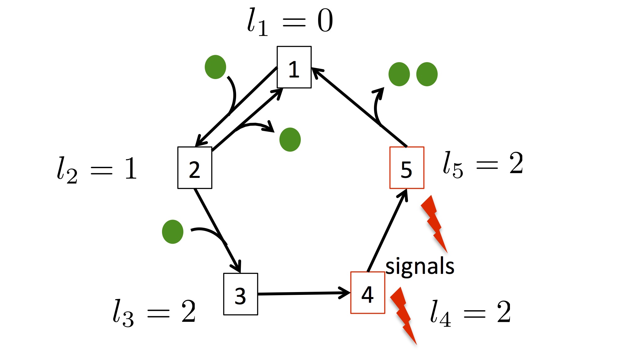
Figure 1: An example of the transition networks of a receptor ($M=5$ and $R=6$). Ligands are represented as green circles and receptor states as square boxes. A subset of the states generates signals indicating ligand concentrations.

The (deterministic) dynamics of the coupled system of the receptor (at ${\mathbf{x}}=\mathbb{0}$) and ligand molecules is described by

$$\frac{\partial c}{\partial t} =D\nabla^{2}_{3d}\,c-\delta^{(3d)}({\mathbf{x}})\frac{d}{dt}\sum_{m}l_{m}n_{m},$$ (2)

$$\frac{dn_{m}}{dt} =\sum_{r}\nu_{m,r}k_{r}n_{\alpha(r)},$$ (3)

where $n_{m}(t)$ is the fraction of the $m$-th receptor state ($0\leq n_{m}(t)\leq 1$), and $k_{r}$ is the rate constant of the $r$-th reaction. $k_{r}$ depends on the ligand concentration, $c({\mathbf{x}}=0,t)$, at the receptor site if $r$ is a ligand-binding reaction (i.e., $l_{\beta(r)}-l_{\alpha(r)}>0$). $\delta^{(3d)}({\mathbf{x}})$ represents the three-dimensional Dirac delta function.

Suppose that the system is in a steady state specified by $c({\mathbf{x}},t)=\bar{c}$ and $n_{m}=\bar{n}_{m}$. $\bar{n}_{m}$ is determined explicitly as a function of rate constants as $\bar{n}_{m}(\{\bar{k}_{r}\})$ by solving (3), where the ligand-concentration dependence enters implicitly through $\bar{k}_{r}=k_{r}|_{c=\bar{c}}$. By linearizing the system around the steady state and including stochastic fluctuations VK , we obtain the following Langevin equations:

$$\frac{\partial\delta c}{\partial t} =D\nabla^{2}_{3d}\,\delta c-\delta^{(3d)}({\mathbf{x}})\frac{d}{dt}\sum_{m}l_{m}\delta n_{m}-{\mathbf{\nabla}}_{3d}\cdot{\mathbf{J}},$$ (4)

$$\frac{d\delta n_{m}}{dt} =\sum_{r}\nu_{m,r}\biggl{(}\bar{k}_{r}\delta n_{\alpha(r)}+\bar{k}^{\prime}_{r}\bar{n}_{\alpha(r)}\delta c({\mathbf{x}}=0,t)\biggr{)}$$

$$+\sum_{r}\nu_{m,r}\xi_{r}.$$ (5)

Here, $\bar{k}^{\prime}_{r}\equiv\partial k_{r}(c)/\partial c|_{c=\bar{c}}$ is nonzero only when the $r$-th reaction is a ligand-binding reaction. $\xi_{r}$ represents the noise associated with the $r$-th reaction, satisfying

$$\langle\xi_{r}(t)\xi_{r^{\prime}}(t^{\prime})\rangle=\delta_{r,r^{\prime}}\bar{k}_{r}\bar{n}_{\alpha(r)}\delta(t-t^{\prime}),$$ (6)

and ${\mathbf{J}}(t,{\mathbf{x}})=(J_{x},J_{y},J_{z})$ is the diffusional noise, satisfying

$$\langle J_{i}(t,{\mathbf{x}})J_{j}(t^{\prime},{\mathbf{x}}^{\prime})\rangle=2D\bar{c}\,\delta_{i,j}\delta(t-t^{\prime})\delta^{(3)}({\mathbf{x}}-{\mathbf{x}}^{\prime}).$$ (7)

The term $-\nabla\cdot J$ in (4) and (7) can be derived by regarding the diffusional process as a special type of “reaction”, where a molecule at a site (in the three dimensional space) is “produced” from one located at a neighboring site, and by using van Kampen’s size expansion Gardiner ; ZOS (see also Fancher ).

By applying the Fourier transform to Eqns. (4) and (5), we obtain

$$-i\omega\sum_{m^{\prime}}(\delta_{m,m^{\prime}}-l_{m^{\prime}}\tau_{c})\widetilde{\delta n}_{m^{\prime}}-\sum_{r}\nu_{m,r}\bar{k}_{r}\widetilde{\delta n}_{\alpha(r)}$$

$$=\sum_{r}\nu_{m,r}[\bar{k}^{\prime}_{r}\bar{n}_{\alpha(r)}\widetilde{\mathcal{J}}+\widetilde{\xi}_{r}],$$ (8)

where

$$\tau_{c}(\omega) \equiv\frac{1}{\bar{c}}\int\frac{d^{3}k}{(2\pi)^{3}}\frac{1}{-i\omega+D{\mathbf{k}^{2}}}\approx\frac{\Lambda}{2\pi^{2}D\bar{c}},$$ (9)

$$\widetilde{\mathcal{J}}(\omega) \equiv\int\frac{d^{3}k}{(2\pi)^{3}}\frac{-i{\mathbf{k}}\cdot\widetilde{\mathbf{J}}}{-i\omega+D{\mathbf{k}^{2}}}.$$ (10)

In (9), we have evaluated the integral at low frequency ($\omega\ll D\Lambda^{2}$) by introducing a UV cutoff, $\Lambda$, corresponding to the inverse of the receptor size as in WS1 . $\tau_{c}$ represents the time-scale associated with ligand molecules diffusing around the receptor. $\widetilde{\mathcal{J}}$ represents the effective diffusional noise “felt” by the receptor, satisfying when $\omega\ll D\Lambda^{2}$,

$$\langle\widetilde{\mathcal{J}}(\omega)\widetilde{\mathcal{J}}(\omega^{\prime})\rangle \approx 2\pi(2\tau_{c}\bar{c}^{2})\delta(\omega+\omega^{\prime}),$$ (11)

where we used (7) and (9).

For ligand-concentration sensitivity, a relevant object is the spectral density, $S_{mm^{\prime}}(\omega)$, defined as $\langle\widetilde{\delta n_{m}}(\omega)\widetilde{\delta n}_{m^{\prime}}(\omega^{\prime})\rangle=2\pi\,S_{mm^{\prime}}(\omega)\,\delta(\omega+\omega^{\prime}).$ Although we can straightforwardly compute this from (8), the analytic computation is difficult for general receptor dynamics. For our purpose, we need only the long-term behavior (i.e., $S_{mm^{\prime}}(\omega=0)$), which can be determined indirectly, as shown below.

In the low-frequency region, by dropping the terms proportional to $\omega$, (8) can be simplified as

$$-\sum_{r}\nu_{m,r}\bar{k}_{r}\widetilde{\delta n}_{\alpha(r)}\approx\sum_{r}\nu_{m,r}(\bar{k}^{\prime}_{r}\bar{n}_{\alpha(r)}\widetilde{\mathcal{J}}+\widetilde{\xi}_{r}).$$ (12)

In contrast to (8), it is no longer possible to invert the left-hand side of (12), because the coefficient matrix, $\nu_{m,r}\bar{k}_{r}$, on the left-hand side is rank-deficient due to the conservation $\sum_{m}\frac{d}{dt}n_{m}=0$. One naive way to avoid this difficulty is to eliminate one of the $M$ variables by using $\widetilde{\delta n}_{m}=-\sum_{m^{\prime}\neq m}\widetilde{\delta n}_{m^{\prime}}$ and express (12) in terms of the remaining $M-1$ variables. However, this asymmetric treatment of variables is inconvenient for the derivation of general formulas.

A key step in our approach is to make use of the following relationships satisfied by $\frac{\partial\bar{n}_{m}}{\partial\bar{c}}$ and $\frac{\partial\bar{n}_{m}}{\partial\bar{k}_{r}}$,

$$-\sum_{r}\nu_{m,r}\bar{k}_{r}\frac{\partial\bar{n}_{\alpha(r)}}{\partial\bar{c}} =\sum_{r}\nu_{m,r}\bar{k}^{\prime}_{r}\bar{n}_{\alpha(r)},$$

$$-\sum_{r}\nu_{m,r}\bar{k}_{r}\frac{\partial\bar{n}_{\alpha(r)}}{\partial\bar{k}_{r^{\prime}}} =\nu_{m,r^{\prime}}\bar{n}_{\alpha(r^{\prime})},$$ (13)

which can be easily obtained from (3). The comparison of the coefficients in (12) and (13) implies that (12) can be expressed as

$$\widetilde{\delta n}_{m}\approx{\frac{\partial\bar{n}_{m}}{\partial\bar{c}}}\widetilde{\mathcal{J}}+\sum_{r}\frac{1}{\bar{n}_{\alpha(r)}}\frac{\partial\bar{n}_{m}}{\partial\bar{k}_{r}}{\tilde{\xi}}_{r}.$$ (14)

See the Appendix for a more rigorous derivation of (14). The physical meaning of the step from (12) to (14) is that, the low-frequency fluctuations $\widetilde{\delta n}_{m}(\omega\approx 0)$ can be determined from the dependences of the steady state on external parameters, $\bar{c}$ and $\bar{k}_{r}$. We call the derivatives $\frac{\partial\bar{n}_{m}}{\partial\bar{c}}$ and $\frac{\partial\bar{n}_{m}}{\partial\bar{k}_{r}}$ the susceptibilities of the steady states to $\bar{c}$ and $\bar{k}_{r}$, respectively.

Finally, from (6), (11), and (14), we obtain

$$S_{m,m^{\prime}}(\omega=0)=2\tau_{c}\bar{c}^{2}\frac{\partial\bar{n}_{m}}{\partial\bar{c}}\frac{\partial\bar{n}_{m^{\prime}}}{\partial\bar{c}}+S^{reac}_{m,m^{\prime}},$$ (15)

where

$$S^{reac}_{m,m^{\prime}}\equiv\sum_{r}\frac{\bar{k}_{r}}{\bar{n}_{\alpha(r)}}\frac{\partial\bar{n}_{m}}{\partial\bar{k}_{r}}\frac{\partial\bar{n}_{m^{\prime}}}{\partial\bar{k}_{r}}$$ (16)

represents the contribution from the reaction noises, $\xi_{r}$.

Similar to WS1 ; WS2 ; Wingreen5 ; Wingreen6 , we assume that the cell “averages” the receptor states over a long-term period, $T$, and quantify the sensitivity of ligand concentration, $\Delta c$, based on the signal-to-noise ratio (SNR). Therefore, we analyze the time-averaged fluctuations

$$\delta N_{m}\equiv\frac{1}{T}\int\,dt\,\delta n_{m}(t),$$ (17)

and the variances

$$C_{m,m^{\prime}}\equiv\langle\delta N_{m}\delta N_{m^{\prime}}\rangle=\frac{1}{T}S_{mm^{\prime}}(\omega=0).$$ (18)

Suppose that a subset of receptor states (active states), ${\mathcal{M}}_{a}\subset\{1,\cdots,M\}$, generates signals indicating the ligand concentration. The maximum SNR is then given by

$$SNR=\sum_{m,m^{\prime}\in{\mathcal{M}}_{a}}\frac{\partial\bar{n}_{m}}{\partial\bar{c}}(C^{-1})_{m,m^{\prime}}\frac{\partial\bar{n}_{m^{\prime}}}{\partial\bar{c}}(\Delta c)^{2}.$$ (19)

The maximum sensitivity (or resolution) can be estimated from the point at which the $SNR$ equals one, which leads to

$$\left(\frac{\Delta c}{\bar{c}}\right)^{2} =\frac{1}{T}\frac{1}{\bar{c}^{2}}\frac{1}{{\sum_{m,m^{\prime}\in{\mathcal{M}}_{a}}\frac{\partial\bar{n}_{m}}{\partial\bar{c}}S^{-1}_{m,m^{\prime}}\frac{\partial\bar{n}_{m^{\prime}}}{\partial\bar{c}}}}.$$ (20)

By plugging (15) into (20) with some matrix manipulation, the maximum sensitivity becomes

$$\left(\frac{\Delta c}{\bar{c}}\right)^{2}=\frac{2\tau_{c}}{T}+\frac{1}{T\bar{c}^{2}}\frac{1}{\sum_{m,m^{\prime}\in{\mathcal{M}}_{a}}\frac{\partial\bar{n}_{m}}{\partial\bar{c}}(S^{reac})^{-1}_{m,m^{\prime}}\frac{\partial\bar{n}_{m^{\prime}}}{\partial\bar{c}}}.$$ (21)

The first term is the same as the BP limit, and the receptor kinetics enters into the second term, which is positive-definite, because $S^{reac}$ is a covariance matrix. Therefore, we have proven that the sensitivity is bounded by the BP limit, regardless of whether the receptor dynamics is in an equilibrium state or a non-equilibrium state.

If, as is usually assumed, all ligand-binding rates are proportional to $\bar{c}$, the second term in (21) can be written as

$$\frac{1}{T}\frac{1}{\sum_{r,r^{\prime}\in l.b.}\sum_{m,m^{\prime}\in{\mathcal{M}}_{a}}\bar{k}_{r}\frac{\partial\bar{n}_{m}}{\partial\bar{k}_{r}}(S^{reac})^{-1}_{m,m^{\prime}}\bar{k}_{r^{\prime}}\frac{\partial\bar{n}_{m^{\prime}}}{\partial\bar{k}_{r^{\prime}}}},$$ (22)

where the summation of reactions, $r,r^{\prime}$, runs over all ligand-binding reactions (l.b.). By utilizing a technique developed in Mochizuki_main ; monomolecular_main ; OM_main , the denominator in (22) can be determined from the state-transition network of the receptor dynamics and expressed as a rational function of rate constants, $\bar{k}_{r}$ (see Appendix for details). Such an explicit formula for arbitrary single-receptor dynamics does not exist in the literature. This enables us to evaluate the sensitivity systematically, even for receptors with complex dynamics.

As an illustration, we first examine a simple receptor model studied by Bialek and Setayeshgar in WS1 . In this model, the receptor has two states: a ligand-unbound ($m=1$) and -bound state ($m=2$). The receptor dynamics is described by

$$\frac{d}{dt}\begin{pmatrix}n_{1}\\ n_{2}\end{pmatrix}=\begin{pmatrix}-k_{1}&k_{-1}\\ k_{1}&-k_{-1}\end{pmatrix}\begin{pmatrix}n_{1}\\ n_{2}\end{pmatrix},$$ (23)

with $k_{1}=k^{\prime}_{1}c$. We assume that the cell “estimates” the ligand concentration from $n_{2}$ (i.e., ${\mathcal{M}}_{a}=\{2\}$). Note that the resulting sensitivity is the same for ${\mathcal{M}}_{a}=\{1\}$, because $\delta n_{1}=-\delta n_{2}$. The maximum sensitivity (21) becomes

$$\left(\frac{\Delta c}{\bar{c}}\right)^{2}=\frac{2\tau_{c}}{T}+\frac{1}{T}\frac{2(\bar{k}_{1}+k_{-1})}{\bar{k}_{1}k_{-1}},$$ (24)

which agrees exactly with the result derived from the FDT in WS1 . We note that, although the approach based on the FDT gives only the sum of the two terms in (24), our method determines them separately, which makes clear the physical origins of these two terms: the contribution from the effective diffusional noise, $\mathcal{J}$, and from the reaction noises, $\xi_{r}$, respectively.

For more nontrivial and biologically relevant receptor dynamics, we consider a kinetic proofreading model Mc and compare this model with the reversible-reaction analogue (Fig. 2). The kinetic proofreading model was originally proposed to explain the ability of T-cell receptors to discriminate foreign antigens from self-antigens based on relatively small differences in ligand affinities. Similar to the kinetic proofreading model of DNA synthesis HF , this model utilizes multiple irreversible steps, resulting in large differences in the production of active states depending on affinity. We remark that we here examine the sensitivity to a single ligand concentration. For a receptor model interacting with spurious ligands, see Mora .

In the kinetic proofreading model, the bare receptor binds with a ligand molecule (with rate $k_{1}=k^{\prime}c$), and the ligand-bound state is then phosphorylated up to $M-2$ times (with rate $k_{p}$ for each modification). The phosphorylated states revert to the unbound state with transition rate $k_{-1}$. By contrast, the reversible model consists of a ligand-binding reaction (with rate $k_{1}=k^{\prime}c$), $M-2$ forward reactions (with rate $k_{p}$), and $M-1$ backward reactions (with rate $k_{-1}$).

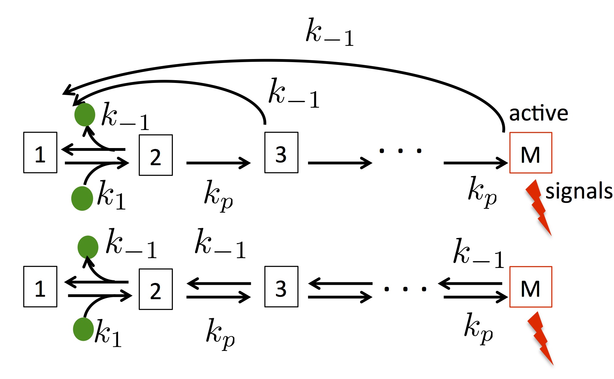
Figure 2: Receptor networks of the kinetic proofreading and reversible models. In both models, we assume that only the $M$-th state is active and generates signals.

We assume that only the final state is active and sends signals indicating ligand concentrations (i.e., ${\mathcal{M}}_{a}=\{M\}$). Introducing the dimensionless parameters $\kappa_{1},\kappa_{-1}$ as

$$k_{1}=\kappa_{1}k_{p},\ \ k_{-1}=\kappa_{-1}k_{p},$$ (25)

we can express the maximum sensitivity, (21), in the following form:

$$\left(\frac{\Delta c}{\bar{c}}\right)^{2} =\frac{2\tau_{c}}{T}+\frac{F_{M}({\kappa_{1},\kappa_{-1}})}{k_{p}T},$$ (26)

where $F_{M}$ is a dimensionless factor that depends on $\kappa_{1},\kappa_{-1}$ (see the Appendix for the explicit expression of $F_{M}$).

Before presenting the numerical results, we estimate the two terms in (26) for acceptably accurate sensing. Thus far, we have considered a single receptor. When a cell has many independent receptors, the sensing accuracy of the entire cell is estimated by dividing (26) by the total number of receptors expressed on the cell surface, which we assume to be $\sim 10^{4}$. We estimate $\tau_{c}=10^{-1}-10^{3}\,{\rm sec}$, (we used $D=10^{-1}-10^{1}{\rm\mu m^{2}/sec}$, a linear dimension of receptor $a\equiv\frac{\Lambda}{\pi}\sim 10^{-2}{\rm{\mu m}}$, and $\bar{c}=10^{2}-10^{4}/{\rm\mu m^{3}}$), and the rate constant $k_{p}=10^{-3}-10^{-1}\,{\rm sec}^{-1}$ (see para1 ; para2 ; para3 for this estimate). Using these values, while the first term in (26) is acceptably small for the integration times $T\sim\,10^{3}\,and{\rm sec}$, the second term can become $\mathcal{O}(1)$ only if $F_{M}<10^{6}$. Therefore, in the following, we focus on the receptor-dependent part in (26), $F_{M}$.

Fig. 3 shows the numerical results of $F_{M=8}(\kappa_{1},\kappa_{-1})$ in the two models.

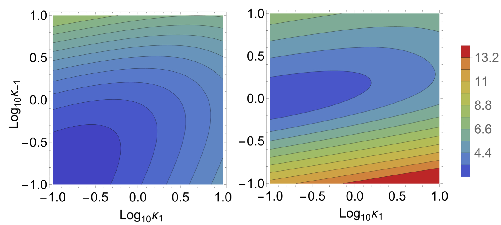
Figure 3: The numerical result of $\log_{10}F_{M}$ for $M=8$ in the kinetic proofreading model (left) and in the reversible model (right). Roughly, $F_{M}<10^{6}$ is required for accurate estimation of ligand-concentration changes.

In the region of $\kappa_{-1}>1$ (the upper-half region of Fig. 3) corresponding to rapid dissociation, the sensitivities in both models behave in a qualitatively similar way: $F_{M}$ is large, except for $\kappa_{-1}\sim 1$, and, as $\kappa_{-1}$ increases, $F_{M}$ becomes larger (or the sensitivity becomes worse) rapidly. By contrast, in the region of $\kappa_{-1}<1$, corr esponding to slow dissociation, the behaviors differ qualitatively between the two models. While $F_{M}$ is large in the reversible models, $F_{M}$ does not depend significantly upon $\kappa_{-1}$ and remains at a lower level in the kinetic proofreading model. Therefore, when $\kappa_{-1}<1$ in the kinetic proofreading model, an accurate sensing is possible over a wide range of $\kappa_{1}$ or, equivalently, ligand-concentration, because $\kappa_{1}=\frac{k^{\prime}\bar{c}}{k_{p}}$.

Next, we examine the dependence of $F_{M}$ on the length of the reaction chains, $M$ (see Fig. 4 (Left)). For simplicity of analysis, we set $\kappa_{1}=1$. From the analytical expression of $F_{M}$ in the Appendix, we can show that in both models, $F_{M}$ asymptotically approaches $F_{M}\sim 2\kappa_{-1}^{\ M-2}$ when $\kappa_{-1}\gg 1$, deteriorating the sensitivity exponentially as $M$ becomes large. However, when $\kappa_{-1}\ll 1$ and while $F_{M}\sim 2/\kappa_{-1}^{M-3}$ is in the reversible model, which is again exponential in $M$, $F_{M}\sim M(M-1)/\kappa_{-1}$ in the kinetic proofreading model, which depends on $M$ only algebraically. Therefore, when $\kappa_{-1}<1$ and $M$ is large, the sensitivity is much higher in the kinetic proofreading model, compared with the reversible model. Note that in either model, for fixed $\kappa_{-1}$, the sensitivity declines monotonically as $M$ increases.

From where does the discrepancy in performance between the two models originate? The sensitivity is determined form the ratio between the (squared) susceptibility, $(\bar{k}_{1}\partial\bar{n}_{M}/\partial\bar{k}_{1})^{2}$, and the fluctuation, $S^{reac}_{M,M}$ (see (22)). As shown in Fig. 4 (right), the value of $S^{reac}_{M,M}$ does not differ significantly between the two models. Therefore, the higher accuracy in the kinetic proofreading model essentially derives from its higher susceptibility, which can be understood as follows: In the reversible model, $\bar{n}_{i}/\bar{n}_{i-1}=\frac{1}{\kappa_{-1}}$ for $i=3,\ldots,M$. Therefore, when $\kappa_{-1}<1$, the dependence of $\bar{n}_{M}$ on $\bar{k}_{1}$ diminishes along the long reaction chain, because a large factor, $\frac{1}{\kappa_{-1}}$, is multiplied in each step toward the active state. By contrast, in the kinetic proofreading model, $\bar{n}_{i}/\bar{n}_{i-1}=\frac{1}{1+\kappa_{-1}}$ for $i=3,\ldots,M-1$, which is not large when $\kappa_{-1}<1$. Therefore, the dependence on $\bar{k}_{1}$ is maintained along the reaction chain.

We note that, in the study of T-cell receptors in Mc , it is the susceptibility to the dissociation constant, $\partial\bar{n}_{M}/\partial k_{-1}$, that leads to T-cell receptor selectivity. However, what we have discussed here is the susceptibility to ligand concentration, $\partial\bar{n}_{M}/\partial\bar{k}_{1}$, which is relevant for the sensitivity to ligand concentration.

In summary, for precise sensing, the receptor does not allow many intermediate modification steps in the broad range of $\kappa_{-1}$ in the reversible model. However, in the kinetic proofreading model, precise sensing is compatible with many internal states, as long as $\kappa_{-1}<1$.

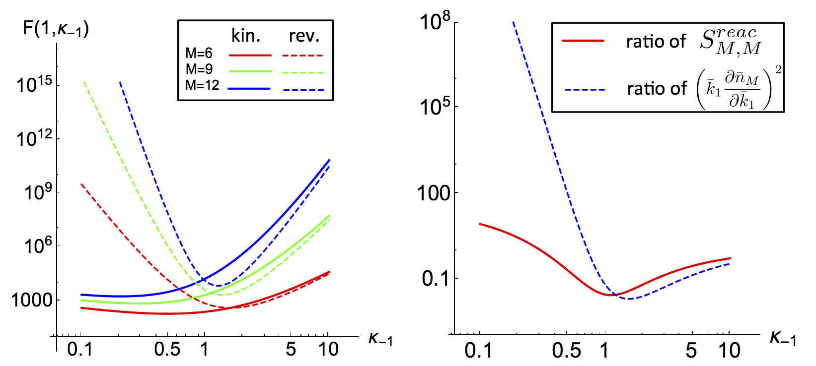
Figure 4: (Left) $F_{M}(1,\kappa_{-1})$ for $M=6,9,12$ in the kinetic proofreading model (thick lines) and the reversible model (dashed lines). (Right) The thick and dashed lines represent the ratios $X_{kin.\,proof.}/X_{rev.}$ between the two models for $X=S^{reac}_{M,M}$ and $(\bar{k}_{1}\frac{\partial\bar{n}_{M}}{\partial\bar{k}_{1}})^{2}$, respectively.

In this Letter, we have derived a general formula for sensitivity, (21), by explicitly accounting for diffusional and reaction noises and utilizing a similar method developed in Mochizuki_main ; monomolecular_main ; OM_main . The sensitivity formula (21) consists of the BP limit and the term determined from the network topology of receptor dynamics. Our result is novel in that the assumption of thermal equilibrium is not required, and the formula is applicable to any instance of receptor dynamics.

The framework of stochastic diffusion equations can serve as the basis for further research into more complex, realistic ligand-receptor dynamics investigations. For example, a potential generalization is the case where, in addition to the ligand the receptor estimates its concentration, the receptor is regulated by other (freely diffusing) ligand species. In this case, as shown in Appendix, $S^{reac}$ in (21) is replaced by

$$S^{reac}_{m,m^{\prime}}\rightarrow S^{reac}_{m,m^{\prime}}+\sum_{i}2\tau_{i}\bar{c}_{i}^{2}\left(\frac{\partial\bar{n}_{m}}{\partial\bar{c}_{i}}\right)^{2},$$ (27)

where $i$ labels other ligand species with concentration $\bar{c}_{i}$ and diffusion constant $D_{i}$, and $\tau_{i}\equiv\frac{\Lambda}{2\pi^{2}D_{i}\bar{c}_{i}}$. We can also investigate reacting ligands by replacing (2) by reaction-diffusion equations. Another biologically relevant and theoretically challenging extension involves dynamically interacting receptors, for example, through ligand-regulated oligomerizations, as in the epidermal growth factor (EGF) receptors HH . We hope to report progress in these directions in the near future.

This work was partially supported by the CREST, Japan Science and Technology Agency. We also express our appreciation to Michio Hitoshima, Atsushi Mochizuki, Alan.D. Rendall, and Yasushi Sako for their inspiring discussions related to this work.

References

- (1) H. C. Berg, and E. M. Purcell, Biophysical journal 20.2 (1977): 193-219.
- (2) W. Bialek, and S. Setayeshgar, Proceedings of the National Academy of Sciences of the United States of America 102.29 (2005): 10040-10045.
- (3) R. Kubo, Reports on Progress in Physics 29.1 (1966): 255.
- (4) W. Bialek, and S. Setayeshgar, physical Review Letters 100.25 (2008): 258101.
- (5) K. Kaizu et al., Biophysical journal 106.4 (2014): 976-985.
- (6) R.G. Endres, and N. S. Wingreen, Proceedings of the National Academy of Sciences 105.41 (2008): 15749-15754.
- (7) R.G. Endres, and N. S. Wingreen, Physical Review Letters 103.15 (2009): 158101.
- (8) T. Mora, and N. S. Wingreen, Physical Review Letters 104.24 (2010): 248101.
- (9) Skoge, Monica, Yigal Meir, and Ned S. Wingreen, Physical review letters 107.17 (2011): 178101.
- (10) V Sourjik, and NS Wingreen, Current opinion in cell biology 24.2 (2012): 262-268.
- (11) M. Skoge, et al. , Physical Review Letters 110.24 (2013): 248102.
- (12) G. Aquino, and R. G. Endres, Physical Review E 81.2 (2010): 021909.
- (13) G. Aquino, and R. G. Endres, Physical Review E 82.4 (2010): 041902.
- (14) T. Mora, Physical Review Letters 115.3 (2015): 038102.
- (15) W. J. Rappel, and H. Levine, Proceedings of the National Academy of Sciences 105.49 (2008): 19270-19275.
- (16) W. J. Rappel, and H. Levine, Physical Review Letters 100.22 (2008): 228101.
- (17) B. Hu, W. Chen, W. J. Rappel, and H. Levine, Physical Review Letters 105.4 (2010): 048104.
- (18) C. C. Govern, and P. R. ten Wolde. Physical review letters 113.25 (2014): 258102.
- (19) A. H. Lang, C.K. Fisher, and T. Mora, Physical review letters 113.14 (2014): 148103.
- (20) S. Fancher, and A. Mugler. Physical Review Letters 118.7 (2017): 078101.
- (21) J. J. Hopfield, Proceedings of the National Academy of Sciences 71.10 (1974): 4135-4139.
- (22) N.G. van Kampen, Canadian journal of physics 39.4 (1961): 551-567.
- (23) De Zarate, Jose M. Ortiz, and Jan V. Sengers, Hydrodynamic fluctuations in fluids and fluid mixtures. Elsevier Science, Amsterdam Netherlands, 2006.
- (24) Gardiner, Crispin W. Stochastic methods. Springer-Verlag, Berlin-Heidelberg-New York-Tokyo, 1985.
- (25) A. Mochizuki, and B. Fiedler, Journal of theoretical biology, 367 (2015), 189-202.
- (26) B. Fiedler, and A. Mochizuki, Mathematical methods in the applied sciences, 38 (2015): 3381-3600.
- (27) T. Okada, and A. Mochizuki, Physical Review Letters 117.4 (2016): 048101.
- (28) T. W. Mckeithan, Proceedings of the national academy of sciences 92.11 (1995): 5042-5046.
- (29) J. D. Stone, A. S. Chervin, and D. M. Kranz, Immunology 126.2 (2009): 165-176.
- (30) M. Hsieh et al., BMC systems biology 4.1 (2010): 57.
- (31) H. Shankaran, H. S. Wiley, and H. Resat, Biophysical journal 90.11 (2006): 3993-4009.
- (32) C. H. Heldin, Cell 80.2 (1995): 213-223.