Discriminative Cooperative Networks for Detecting Phase Transitions
Abstract
The classification of states of matter and their corresponding phase transitions is a special kind of machine-learning task, where physical data allow for the analysis of new algorithms, which have not been considered in the general computer-science setting so far. Here we introduce an unsupervised machine-learning scheme for detecting phase transitions with a pair of discriminative cooperative networks (DCN). In this scheme, a guesser network and a learner network cooperate to detect phase transitions from fully unlabeled data. The new scheme is efficient enough for dealing with phase diagrams in two-dimensional parameter spaces, where we can utilize an active contour model – the snake – from computer vision to host the two networks. The snake, with a DCN “brain”, moves and learns actively in the parameter space, and locates phase boundaries automatically.
The richness of states of matter, together with the power of machine-learning techniques for recognizing and representing patterns, are revealing new methods for studying emergent phenomena in condensed matter physics. Paradigms in machine learning have been nicely mapped to those in physics. For example, the classification techniques in machine learning have been applied in detecting classical and quantum phase transitions Carrasquilla and Melko (2017); Wang (2016); Ch’ng et al. (2017); Broecker et al. (2017); van Nieuwenburg et al. (2017); Schindler et al. (2017); Wetzel and Scherzer (2017); Wetzel (2017); Ohtsuki and Ohtsuki (2016); Broecker et al. ; Costa et al. (2017); Ch’ng et al. (2018); Rao et al. ; Li et al. , the artificial-neural-network architecture has inspired a high-quality Ansatz for many-body wave functions Carleo and Troyer (2017); Deng et al. (2017); Chen et al. ; Gao and Duan (2017); Torlai et al. ; Cai and Liu (2018); Nomura et al. (2017); Glasser et al. (2018), the generative power of energy-based statistical models is utilized to accelerate Monte Carlo simulations Wang (2017); Huang et al. (2017); Huang and Wang (2017); Fujita et al. ; Liu et al. (2017a, b); Xu et al. (2017); Nagai et al. (2017), and regression has aided material-property prediction Rupp et al. (2012); Faber et al. (2016); Pilania et al. (2013); Arsenault et al. (2014, ); Bartók et al. (2017); Brockherde et al. (2017). Moreover, basic notions from both physics and machine learning can mutually inspire new insights, e.g. a relation between deep learning and the renormalization group Landon-Cardinal and Poulin (2012); Bény ; Mehta and Schwab ; Lin et al. (2017); Rolnick and Tegmark ; Koch-Janusz and Ringel .
In physics, the phase (e.g. magnetic vs. non-magnetic phase) is most efficient in summarizing material properties. When changing tuning parameters (e.g. temperature), the material properties may change discontinuously, which is called a phase transition. Machine-learning phase transitions is possible from two angles. In the supervised approach, physics knowledge is used to provide answers in limiting cases and the machine learner is asked to extrapolate to the transition point Carrasquilla and Melko (2017). In the unsupervised approach, no such knowledge is assumed and the transition is sought by other means Wang (2016); Wetzel and Scherzer (2017); Costa et al. (2017); Ch’ng et al. (2018).
The confusion scheme proposed previously by us is a hybrid method van Nieuwenburg et al. (2017), where no knowledge of the limiting cases is needed but the learning is still carried out in a supervised manner. Specifically, one first guesses a transition point and tries to train the machine with this guess. When the guess is correct, the machine learner achieves the highest performance. Here we gain the ability to find transitions at the cost of having to repeat the training for many guesses, which is computationally expensive.
In this work, we extend the confusion scheme by training a “guesser” together with the “learner”. This leads to a fully automated scheme – the discriminative cooperative networks (DCN). In addition, phase transitions in two-dimensional (2D) parameter spaces share many common aspects with image-feature detection in computer vision. However in images the data are the colors, whereas in physics they can be arbitrary results of measurements whose features might not be apparent to the human eyes. This inspires us to use an active contour method Kass et al. (1988), combined with the DCN scheme, to perform automated searching of phase boundaries in 2D phase diagrams.
We consider data that can be ordered along a tuning parameter . At various values of the data are described by , and can be thought of as a vector of real numbers – results of physical measurements at . We describe a neural network on an abstract level as a map that takes data and infers the probability distribution , where represents the probability of belonging to phase . Since the data are indexed by , this can be simplified by considering the probability distribution directly on . At each only a single probability (corresponding to the correct phase) should equal to unity, and the rest zero. With phase transitions, the distribution varies with discontinuously, e.g. for a transition at between two phases A and B there are two components and , where is the Heaviside step-function.
For supervised learning, a large body of with the corresponding correct answer have to be known beforehand, and the neural network is trained with the goal . To achieve this goal, parameters that characterize the neural network are adjusted during training to minimize a cost function , quantifying the mismatch between the network’s prediction and the known answer. depends implicitly on the parameters through and can be minimized using gradient descent methods.
Typical machine-learning data live in high-dimensional feature spaces in an unordered fashion. The number of ways to separate them into two classes is where is the size of the dataset. For phase transitions however, all data are ordered in the parameter space, and for a single transition point, the number of ways is merely . In physics, it is affordable to enumerate all these possibilities to find the most reasonable separation point. This observation led to the confusion scheme van Nieuwenburg et al. (2017), where one guesses the transition point and then train the learner network . By monitoring the number of “correctly” classified samples according to this guess – the performance, the true value for can be deduced. It turns out the true value is the guess for which the performance is optimal, because here the assigned probabilities in and the structures in are the most consistent, such that the learner network is least confused by the training.
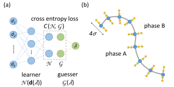
In the previous proposal, we searched for the optimal by a brute-force scan of the parameter space. For phase transitions in higher-dimensional parameter spaces, this approach is inefficient. In this work we introduce the guesser network . It performs the map , representing the probabilities of belonging to each possible phase. That is, now the guesser provides . The guesser is itself characterized by a set of parameters on which we wish to perform gradient descent. The overall cost function of the learner and guesser is now , see Fig. 1(a). In this way, we have promoted the human input to an active agent . During training, the learner tries to learn the data according to the suggested labels obtained from the guesser, and the guesser tries to provide a better set of labels – they cooperatively optimize the cost .
We first assume one-dimensional (1D) parameter space with two phases, and propose a logistic-regression guesser network with one/two input/output neuron(s): , where is the logistic (sigmoid) function, A/B denotes the first/second output neuron, and . The guesser is hence characterized by two parameters and , setting respectively the guessed transition point and the sharpness of the transition. Gradient descent can be performed on both and . We use the cross entropy cost function , which is suitable for classification problems. The gradient of on the guesser network is obtained by the following equations:
| (1) |
These equations fully determine the dynamics of the guesser: and , where and are the learning rates for the two parameters, respectively. The dynamics of the learner follows with another independent learning rate , here the gradient is obtained by the back-propagation algorithm Rumelhart et al. (1986).
At this point, one could conceptually regard the guesser and learner together as one compound agent, capable of self-learning. We call this scheme discriminative cooperative networks (DCN), with the name inspired by the powerful generative adversarial networks (GAN) Goodfellow et al. for generating samples resembling the training data.
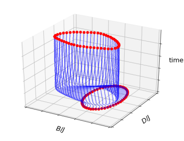
The DCN scheme is efficient because there is no need for repetitive training at each guess. This allows us to move to higher-dimensional parameter spaces. Here we focus on 2D since physics studies usually report phase diagrams in 2D parameter spaces. Inspired by the computer vision techniques for finding image features, we use an active contour model – the snake Kass et al. (1988) – for the parametrization of the guesser.
In computer vision, the snake is a discretized curve of linked nodes, , parametrized by (for closed snakes) or (for open snakes), see Fig. 1(b). The nodes can move actively under “image forces”, which are the minus gradients of an “external energy”, with respect to the snake nodes. Specifically, the external energy is the total potential energy , with the potential proportional to the local color intensity (gradient of color intensity) for line (edge) detection. To keep the snake smooth, internal forces are also introduced, which are derived from the internal energy . Increasing makes for a more “elastic” snake by preventing stretching and a more “solid” snake by preventing bending. The snake evolves in time to lower its total energy , and the equation of motion is implemented numerically Kass et al. (1988).
In this work, we combine the DCN scheme in artificial intelligence with the snake in computer vision, and the result is an intelligent snake. To do this, we replace the conventional image force in computer vision with the machine-learning gradient . The 1D DCN scheme requires training data from both sides of the guessed transition point. This implies, for the 2D case, a width of the snake. The width, denoted again by , is generically different at each node, and enables the snake to sense its surroundings by selecting training samples in its vicinity within this length scale, as shown in Fig. 1(b). Specifically the sample points are drawn at each node perpendicularly to the snake, with distances uniformly picked in . The 2D guesser function is then locally the same as in the 1D case, evaluated by each node in its perpendicular direction. For implementation details, see 111The source code can be found in https://github.com/rhinech/snake.. We note the probing of data within a window (in searching for distinct phases) is a powerful concept that is also successfully used in Ref. Broecker et al. .
Ising model.
We test our scheme on 1D parameter space by studying the classical Ising model on the square lattice:
| (2) |
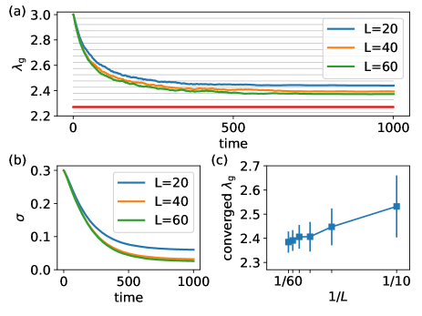
where are the Ising spins, denotes nearest neighbors with coupling , and the tuning parameter is the temperature . This model has a thermal phase transition from the ferromagnetic phase (with aligned spins) to the paramagnetic phase (with random spins) when the temperature is increased across . The training data are spin configurations drawn from a Monte Carlo simulation on an by square lattice. We select 100 temperatures uniformly from to and prepare 100 samples at each temperature. Every mini-batch consists of random samples, one from each temperature 222We have preprocessed each configuration by flipping all its spins when the net magnetization is negative.. Time is measured by the number of learned mini-batches. During training, the guesser moves toward the exact transition point and decreases the width because the discrimination is sharper and sharper (Fig. 2). does not converge to the exact value when increasing , because the networks most likely learn the order parameter, which is the simplest, but not the sharpest signal for detecting phase transition. It future study we investigate the possibility for the networks to learn also the fluctuations of order parameters.
Bose-Hubbard model.
As a first example for applying the DCN scheme in 2D parameter spaces, we choose the Bose-Hubbard model:
| (3) |
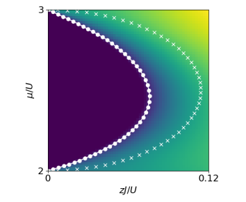
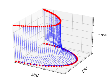
where / is the bosonic creation/annihilation operator. Regarding the Hubbard interaction as the energy unit, for each chemical potential , the model has a quantum phase transition (at zero temperature) from the Mott insulating state to the superfluid state, when the hopping is increased Fisher et al. (1989). A useful indicator of this phase transition is the average hopping where . Note the notion of is unknown to the initial untrained snake, otherwise the problem reduces to computer vision where machine learning is not needed. The critical point reaches local maxima when the system is at commensurate fillings, corresponding to half-integers . A phase diagram of this system results in the series of well-known Mott-lobes. We use the mean-field theory developed in Ref. Krauth et al. (1992) to generate vector data , where with denotes the amplitude for having bosons per site, and a cutoff of is chosen for numerics. We target the third Mott lobe with , and the snake successfully captures the phase boundary as shown in Fig. 3. In this case the phase boundary touches the boundary of the parameter space, so we use an open snake with fixed head and tail at known transition points. The snake’s motion is then restricted to shrinking or expanding. It is important to emphasize here that we have used knowledge of only two points along the axis in the whole phase diagram, and that the training data seen by the snake is not the average hopping as shown in the background, but the vector data mentioned above 333Additionally, we have tested that the snake is capable of finding the lobe from an initially circular (periodic) configuration..
Spin-1 Heisenberg chain.
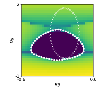
We now move to a quantum phase transition beyond mean-field theory. We choose the spin-1 antiferromagnetic Heisenberg chain with anisotropy and transverse magnetic field:
| (4) |
where are 3 by 3 matrices satisfying . In the 2D parameter space of magnetic field vs. anisotropy , this model has a pocket named the Haldane phase – a topologically nontrivial phase – around zero magnetic field and anisotropy Pollmann et al. (2010). The transition across the boundary of this pocket can be detected by a change in the degeneracy structure of the entanglement spectrum (eigenvalues of the reduced density matrix for part of the spin chain in the ground state), but again the initial untrained snake is unaware of this. For the training data, we simulate an infinite chain with translational invariance using iTEBD Vidal (2007) with bond dimension , and record all eigenvalues of the reduced density matrix when the chain is cut by half at a bond, i.e. . The result is shown in Fig. 3. In this model the phase boundary is closed and located near the center of the parameter space. For this reason we use a closed (periodic) snake whose motion now also contains translation and rotation.
In this paper we have proposed the discriminative cooperative networks, capable of self-consistently finding transition points. The high efficiency of this scheme allows us to explore 2D parameter spaces, where we utilized the snake model from computer vision. Our method is in spirit similar to the actor-critic scheme for reinforcement learning Konda and Tsitsiklis (2003) and the adversarial training scheme for generative models Goodfellow et al. .
The major limitation for the snake is the need for an initial state that has overlap with the desired features to be detected, so that it is able to probe a gradient. This was also true for their use in computer vision. In applications to phase diagrams, we have the clear advantage of some known extreme limits at which we can fix the snake. We can also overcome this problem by scaling/moving the snake.
Ch’ng et al. have proposed to train neural networks deep inside the known phases with supervision, and then use them to extrapolate the whole phase diagram Ch’ng et al. (2017). Such a method is, compared to our method, simpler and faster. However the data for supervised training have to be carefully chosen, otherwise interpolation of the phase boundary could be qualitatively incorrect Ch’ng et al. (2017). On the contrary, the snake can actively explore a much larger area in the parameter space. For general phase transition problems, one could use both methods complementarily.
Machine-learning applications usually assume the existence of big data. However in science it might be expensive to obtain these data. With the DCN scheme, it is possible for a machine-learning agent to suggest parameters for the physicist to carry out experiments/simulations and rapidly locate interesting phenomena. In this paper we put forward a proposal to realize this scheme.
Acknowledgements.
The authors thank L. Wang, S. D. Huber, S. Trebst, K. Hepp, M. Sigrist, and T. M. Rice for reading the manuscript and helpful suggestions. Y.-H.L. thank stimulating discussions with G. Sordi and A.-M. Tremblay. Y.-H.L. is supported by ERC Advanced Grant SIMCOFE and the Canada First Research Excellence Fund. E.v.N. gratefully acknowledges financial support from the Swiss National Science Foundation (SNSF) through grant P2EZP2-172185. The authors used TensorFlow Abadi et al. for machine learning.References
- Carrasquilla and Melko (2017) Juan Carrasquilla and Roger G Melko, “Machine learning phases of matter,” Nat. Phys. 13, 431–434 (2017).
- Wang (2016) Lei Wang, “Discovering phase transitions with unsupervised learning,” Phys. Rev. B 94, 195105 (2016).
- Ch’ng et al. (2017) Kelvin Ch’ng, Juan Carrasquilla, Roger G. Melko, and Ehsan Khatami, “Machine Learning Phases of Strongly Correlated Fermions,” Phys. Rev. X 7, 031038 (2017).
- Broecker et al. (2017) Peter Broecker, Juan Carrasquilla, Roger G. Melko, and Simon Trebst, “Machine learning quantum phases of matter beyond the fermion sign problem,” Scientific Reports 7, 8823 (2017).
- van Nieuwenburg et al. (2017) Evert P. L. van Nieuwenburg, Ye-Hua Liu, and Sebastian D. Huber, “Learning phase transitions by confusion,” Nat. Phys. 13, 435–439 (2017).
- Schindler et al. (2017) Frank Schindler, Nicolas Regnault, and Titus Neupert, “Probing many-body localization with neural networks,” Phys. Rev. B 95, 245134 (2017).
- Wetzel and Scherzer (2017) Sebastian J. Wetzel and Manuel Scherzer, “Machine learning of explicit order parameters: From the Ising model to SU(2) lattice gauge theory,” Phys. Rev. B 96, 184410 (2017).
- Wetzel (2017) Sebastian J. Wetzel, “Unsupervised learning of phase transitions: From principal component analysis to variational autoencoders,” Phys. Rev. E 96, 022140 (2017).
- Ohtsuki and Ohtsuki (2016) Tomoki Ohtsuki and Tomi Ohtsuki, “Deep Learning the Quantum Phase Transitions in Random Two-Dimensional Electron Systems,” J. Phys. Soc. Japan 85, 123706 (2016).
- (10) P. Broecker, F. Assaad, and S. Trebst, “Quantum phase recognition via unsupervised machine learning,” arXiv:1707.00663 .
- Costa et al. (2017) Natanael C. Costa, Wenjian Hu, Z. J. Bai, Richard T. Scalettar, and Rajiv R. P. Singh, “Principal component analysis for fermionic critical points,” Phys. Rev. B 96, 195138 (2017).
- Ch’ng et al. (2018) Kelvin Ch’ng, Nick Vazquez, and Ehsan Khatami, “Unsupervised machine learning account of magnetic transitions in the Hubbard model,” Phys. Rev. E 97, 013306 (2018).
- (13) Wen-Jia Rao, Zhenyu Li, Qiong Zhu, Mingxing Luo, and Xin Wan, “Identifying Product Order with Restricted Boltzmann Machines,” arXiv:1709.02597v1 .
- (14) Zhenyu Li, Mingxing Luo, and Xin Wan, “Extracting Critical Exponent by Finite-Size Scaling with Convolutional Neural Networks,” arXiv:1711.04252v1 .
- Carleo and Troyer (2017) Giuseppe Carleo and Matthias Troyer, “Solving the quantum many-body problem with artificial neural networks,” Science 355, 602–606 (2017).
- Deng et al. (2017) Dong-Ling Deng, Xiaopeng Li, and S. Das Sarma, “Machine learning topological states,” Phys. Rev. B 96, 195145 (2017).
- (17) Jing Chen, Song Cheng, Haidong Xie, Lei Wang, and Tao Xiang, “On the Equivalence of Restricted Boltzmann Machines and Tensor Network States,” arXiv:1701.04831 .
- Gao and Duan (2017) Xun Gao and Lu-Ming Duan, “Efficient representation of quantum many-body states with deep neural networks,” Nature Communications 8, 662 (2017).
- (19) Giacomo Torlai, Guglielmo Mazzola, Juan Carrasquilla, Matthias Troyer, Roger Melko, and Giuseppe Carleo, “Many-body quantum state tomography with neural networks,” arXiv:1703.05334 .
- Cai and Liu (2018) Zi Cai and Jinguo Liu, “Approximating quantum many-body wave functions using artificial neural networks,” Phys. Rev. B 97, 035116 (2018).
- Nomura et al. (2017) Yusuke Nomura, Andrew S. Darmawan, Youhei Yamaji, and Masatoshi Imada, “Restricted boltzmann machine learning for solving strongly correlated quantum systems,” Phys. Rev. B 96, 205152 (2017).
- Glasser et al. (2018) Ivan Glasser, Nicola Pancotti, Moritz August, Ivan D. Rodriguez, and J. Ignacio Cirac, “Neural-network quantum states, string-bond states, and chiral topological states,” Phys. Rev. X 8, 011006 (2018).
- Wang (2017) Lei Wang, “Exploring cluster Monte Carlo updates with Boltzmann machines,” Phys. Rev. E 96, 051301 (2017).
- Huang et al. (2017) Li Huang, Yi-Feng Yang, and Lei Wang, “Recommender engine for continuous-time quantum Monte Carlo methods,” Phys. Rev. E 95, 031301 (2017).
- Huang and Wang (2017) Li Huang and Lei Wang, “Accelerated Monte Carlo simulations with restricted Boltzmann machines,” Phys. Rev. B 95, 035105 (2017).
- (26) Hiroyuki Fujita, Yuya. O. Nakagawa, Sho Sugiura, and Masaki Oshikawa, “Construction of Hamiltonians by machine learning of energy and entanglement spectra,” arXiv:1705.05372 .
- Liu et al. (2017a) Junwei Liu, Yang Qi, Zi Yang Meng, and Liang Fu, “Self-learning Monte Carlo method,” Phys. Rev. B 95, 041101 (2017a).
- Liu et al. (2017b) Junwei Liu, Huitao Shen, Yang Qi, Zi Yang Meng, and Liang Fu, “Self-learning Monte Carlo method and cumulative update in fermion systems,” Phys. Rev. B 95, 241104 (2017b).
- Xu et al. (2017) Xiao Yan Xu, Yang Qi, Junwei Liu, Liang Fu, and Zi Yang Meng, “Self-learning quantum Monte Carlo method in interacting fermion systems,” Phys. Rev. B 96, 041119 (2017).
- Nagai et al. (2017) Yuki Nagai, Huitao Shen, Yang Qi, Junwei Liu, and Liang Fu, “Self-learning Monte Carlo method: Continuous-time algorithm,” Phys. Rev. B 96, 161102 (2017).
- Rupp et al. (2012) Matthias Rupp, Alexandre Tkatchenko, Klaus-Robert Müller, and O. Anatole von Lilienfeld, “Fast and Accurate Modeling of Molecular Atomization Energies with Machine Learning,” Phys. Rev. Lett. 108, 058301 (2012).
- Faber et al. (2016) Felix A. Faber, Alexander Lindmaa, O. Anatole von Lilienfeld, and Rickard Armiento, “Machine Learning Energies of 2 Million Elpasolite (ABC2D6) Crystals,” Phys. Rev. Lett. 117, 135502 (2016).
- Pilania et al. (2013) Ghanshyam Pilania, Chenchen Wang, Xun Jiang, Sanguthevar Rajasekaran, and Ramamurthy Ramprasad, “Accelerating materials property predictions using machine learning,” Sci. Rep. 3, 2810 (2013).
- Arsenault et al. (2014) Louis-François Arsenault, Alejandro Lopez-Bezanilla, O. Anatole von Lilienfeld, and Andrew J. Millis, “Machine learning for many-body physics: The case of the Anderson impurity model,” Phys. Rev. B 90, 155136 (2014).
- (35) Louis-François Arsenault, O Anatole von Lilienfeld, and Andrew J Millis, “Machine learning for many-body physics: efficient solution of dynamical mean-field theory,” arXiv:1506.08858 .
- Bartók et al. (2017) Albert P. Bartók, Sandip De, Carl Poelking, Noam Bernstein, James R. Kermode, Gábor Csányi, and Michele Ceriotti, “Machine learning unifies the modeling of materials and molecules,” Science Advances 3 (2017).
- Brockherde et al. (2017) Felix Brockherde, Leslie Vogt, Li Li, Mark E Tuckerman, Kieron Burke, and Klaus-Robert Müller, “Bypassing the Kohn-Sham equations with machine learning.” Nature Communications 8, 872 (2017).
- Landon-Cardinal and Poulin (2012) Olivier Landon-Cardinal and David Poulin, “Practical learning method for multi-scale entangled states,” New J. Phys. 14, 085004 (2012).
- (39) Cédric Bény, “Deep learning and the renormalization group,” arXiv:1301.3124 .
- (40) Pankaj Mehta and David J. Schwab, “An exact mapping between the Variational Renormalization Group and Deep Learning,” arXiv:1410.3831 .
- Lin et al. (2017) Henry W. Lin, Max Tegmark, and David Rolnick, “Why Does Deep and Cheap Learning Work So Well?” Journal of Statistical Physics 168, 1223–1247 (2017).
- (42) David Rolnick and Max Tegmark, “The power of deeper networks for expressing natural functions,” arXiv:1705.05502 .
- (43) Maciej Koch-Janusz and Zohar Ringel, “Mutual Information, Neural Networks and the Renormalization Group,” arXiv:1704.06279 .
- Kass et al. (1988) Michael Kass, Andrew Witkin, and Demetri Terzopoulos, “Snakes: Active contour models,” Int. J. Comput. Vis. 1, 321–331 (1988).
- Rumelhart et al. (1986) David E. Rumelhart, Geoffrey E. Hinton, and Ronald J. Williams, “Learning representations by back-propagating errors,” Nature 323, 533–536 (1986).
- (46) Sebastian Ruder, “An overview of gradient descent optimization algorithms,” arXiv:1609.04747 .
- (47) Sergey Ioffe and Christian Szegedy, “Batch Normalization: Accelerating Deep Network Training by Reducing Internal Covariate Shift,” arXiv:1502.03167 .
- (48) Ian J. Goodfellow, Jean Pouget-Abadie, Mehdi Mirza, Bing Xu, David Warde-Farley, Sherjil Ozair, Aaron Courville, and Yoshua Bengio, “Generative Adversarial Networks,” arXiv:1406.2661 .
- Note (1) The source code can be found in https://github.com/rhinech/snake.
- Kingma and Ba (2015) Diederik P. Kingma and Jimmy Lei Ba, “Adam: a Method for Stochastic Optimization,” in Int. Conf. Learn. Represent. 2015 (2015) pp. 1–15.
- Note (2) We have preprocessed each configuration by flipping all its spins when the net magnetization is negative.
- Fisher et al. (1989) Matthew P. A. Fisher, Peter B. Weichman, G. Grinstein, and Daniel S. Fisher, “Boson localization and the superfluid-insulator transition,” Phys. Rev. B 40, 546–570 (1989).
- Krauth et al. (1992) Werner Krauth, Michel Caffarel, and Jean-Philippe Bouchaud, “Gutzwiller wave function for a model of strongly interacting bosons,” Phys. Rev. B 45, 3137–3140 (1992).
- Note (3) Additionally, we have tested that the snake is capable of finding the lobe from an initially circular (periodic) configuration.
- Pollmann et al. (2010) Frank Pollmann, Ari M. Turner, Erez Berg, and Masaki Oshikawa, “Entanglement spectrum of a topological phase in one dimension,” Phys. Rev. B 81, 064439 (2010).
- Vidal (2007) G. Vidal, “Classical Simulation of Infinite-Size Quantum Lattice Systems in One Spatial Dimension,” Phys. Rev. Lett. 98, 070201 (2007).
- Konda and Tsitsiklis (2003) Vijay R Konda and John N Tsitsiklis, “Actor-Critic Algorithms,” SIAM J. Control Optim. 42, 1143–1166 (2003).
- (58) Martín Abadi, Ashish Agarwal, Paul Barham, Eugene Brevdo, Zhifeng Chen, Craig Citro, Greg S. Corrado, Andy Davis, Jeffrey Dean, Matthieu Devin, Sanjay Ghemawat, Ian Goodfellow, Andrew Harp, Geoffrey Irving, Michael Isard, Yangqing Jia, Rafal Jozefowicz, Lukasz Kaiser, Manjunath Kudlur, Josh Levenberg, Dan Mane, Rajat Monga, Sherry Moore, Derek Murray, Chris Olah, Mike Schuster, Jonathon Shlens, Benoit Steiner, Ilya Sutskever, Kunal Talwar, Paul Tucker, Vincent Vanhoucke, Vijay Vasudevan, Fernanda Viegas, Oriol Vinyals, Pete Warden, Martin Wattenberg, Martin Wicke, Yuan Yu, and Xiaoqiang Zheng, “TensorFlow: Large-Scale Machine Learning on Heterogeneous Distributed Systems,” arXiv:1603.04467 .