The Matrix Hilbert Space and Its Application to Matrix Learning

Abstract

Theoretical studies have proven that the Hilbert space has remarkable performance in many fields of applications. Frames in tensor product of Hilbert spaces were introduced to generalize the inner product to high-order tensors. However, these techniques require tensor decomposition which could lead to the loss of information and it is a NP-hard problem to determine the rank of tensors. Here, we present a new framework, namely matrix Hilbert space to perform a matrix inner product space when data observations are represented as matrices. We preserve the structure of initial data and multi-way correlation among them is captured in the process. In addition, we extend the reproducing kernel Hilbert space (RKHS) to reproducing kernel matrix Hilbert space (RKMHS) and propose an equivalent condition of the space uses of the certain kernel function. A new family of kernels is introduced in our framework to apply the classifier of Support Tensor Machine(STM) and comparative experiments are performed on a number of real-world datasets to support our contributions.

1 Introduction

The Hilbert space was named after David Hilbert for his fundamental work to generalize the concept of Euclidean space to an infinite dimensional one in the field of functional analysis. With other related works, researchers have made great contribution in the development of quantum mechanics (Birkhoff and Von Neumann, 1936; Sakurai et al, 1995; Ballentine, 2014), partial differential equations (Crandall et al, 1992; Gustafson, 2012; Gilbarg and Trudinger, 2015), Fourier analysis (Stein and Weiss, 2016), spectral theory (Birman and Solomjak, 2012), etc. Many methodologies have been proposed in the literature, but techniques are mainly studied based on infinite vector spaces. Since it is more natural to represent real-world data as high-order tensors, tensor product has become useful in approximating such variables. Khosravi and Asgari (Asgari and Khosravi, 2003) introduced frames in tensor product of Hilbert spaces. It is an extension of tensor product to construct a new Hilbert space of higher order tensors with several existing Hilbert spaces. Meanwhile, bases and frames in Hilbert $C^{*}$-modules with a $C^{*}$-algebra were investigated (Lance, 1995). Tensor product of frames for Hilbert modules produce frames for a new Hilbert module (Khosravi and Khosravi, 2007).

Based on this framework, a reproducing kernel Hilbert space (RKHS) of functions was proposed and proven essential in a number of applications, such as signal processing and detection, as well as statistical learning theory. The reproducing kernel was systematically developed in the early 1950s by Nachman Aronszajn (Aronszajn, 1950) and Stefan Bergman. The notion of kernels in Hilbert spaces wasn’t brought to the field of machine learning until 20th century (Wahba, 1990; Schölkopf et al, 1998; Vapnik and Vapnik, 1998; Boser et al, 1992). The kernel methods expand theories and algorithms well developed for the linear cases to nonlinear methods to detect the kind of dependencies that allow successful prediction of properties of interest (Hofmann et al, 2008).

Most of standard kernels use tensor decomposition to reveal the underlying structure of tensor data (Signoretto et al, 2011; He et al, 2014). Existing tensor-based techniques consist of seeking representative low-dimensional subspaces or sum of rank-1 factor. However, information could be lost in this procedure and it is a NP-hard problem to determine the rank of tensors. Another matrix-based approach (Gao et al, 2015) reformulates the Support Tensor Machine (STM) classifier where a matrix representation (Gao and Wu, 2012) was applied in the construction of kernel function. Its improvement in the performance of classification problems attributes to the matrix kernel function which describes the inner product. Inspired by the above work, we study a new framework in this paper, namely matrix Hilbert space to perform inner product when data observations are represented as matrices. We exploit matrix inner product to capture structural information which could not be completely described by a simple scalar result. This includes in particular the case of Hilbert space where the properties of the scalar inner product are generalized. In addition, we systematically explain the matrix integral based on matrix polynomials (Sinap and Van Assche, 1994) upon our work. We begin by presenting the framework of matrix inner product space and extending it to the concept of matrix Hilbert space. Second, we develop tools extending to our matrix Hilbert space the concept of reproducing kernel matrix Hilbert space (RKMHS). To this end we derive an algorithm through alternating projection procedure to play our kernel trick.

The remainder of the article is structured as follows. In Sect. 2 we present the framework of matrix Hilbert spaces combined with basic inequalities and properties. In Sect. 3 we present definitions of reproducing kernel and corresponding reproducing kernel matrix Hilbert space. In Sect. 4 a new family of kernels is described based on the framework of RKMHS and its performance on benchmark datasets. Finally, we present concluding remarks in Sect. 5.

2 Matrix Inner product

In this section, we present the framework of matrix Hilbert space which extends the scalar inner product to a matrix form. One advantage is that it is a natural generalization of Hilbert space of vectors; this is the case especially when the dimension of the matrix inner product is one by one. Meanwhile, we reformulate some fundamental properties such as Cauchy-Schwarz inequality in our new space and obtain some good results.

In this study, scales are denoted by lowercase letters, e.g., s, vectors by boldface lowercase letters, e.g., v, matrices by boldface capital letters, e.g., M and general sets or spaces by gothic letters, e.g., $\mathcal{B}$. We start with some basic notations defined in the literature.

The Frobenius norm of a matrix $\textbf{X}\in\mathbb{R}^{m\times n}$ is defined by

$$\|\textbf{X}\|=\sqrt{\sum_{i_{1}=1}^{m}\sum_{i_{2}=1}^{n}x_{i_{1}i_{2}}^{2}},$$

which is equal to the Euclidean norm of their vectorized representation.

The spectral norm of a matrix $\textbf{X}\in\mathbb{R}^{m\times n}$ is the square root of the largest eigenvalue of $\textbf{X}^{\intercal}\textbf{X}$:

$$\|\textbf{X}\|_{2}=\sqrt{\lambda_{\max}(\textbf{X}^{\intercal}\textbf{X})},$$

which is a natural norm induced by $l_{2}$ norm.

The inner product of two same-sized matrices $\textbf{X},\textbf{Y}\in\mathbb{R}^{m\times n}$ is defined as the sum of products of their entries, i.e.,

$$\langle\textbf{X},\textbf{Y}\rangle=\sum_{i_{1}=1}^{m}\sum_{i_{2}=1}^{n}x_{i_{1}i_{2}}y_{i_{1}i_{2}}.$$

Now we present our framework of matrix inner product as follows.

Definition 1 (Matrix Inner Product)

Let $\mathcal{H}$ be a real linear space, the matrix inner product is a mapping $\langle\cdot,\cdot\rangle_{\mathcal{H}}:\mathcal{H}\times\mathcal{H}\rightarrow\mathbb{R}^{n\times n}$ satisfying the following properties, for all $\textbf{X},\textbf{X}_{1},\textbf{X}_{2},\textbf{Y}\in\mathcal{H}$

(1) $\langle\textbf{Y},\textbf{X}\rangle_{\mathcal{H}}=\langle\textbf{X},\textbf{Y}\rangle_{\mathcal{H}}^{\intercal}$

(2) $\langle\lambda\textbf{X}_{1}+\mu\textbf{X}_{2},\textbf{Y}\rangle_{\mathcal{H}}=\lambda\langle\textbf{X}_{1},\textbf{Y}\rangle_{\mathcal{H}}+\mu\langle\textbf{X}_{2},\textbf{Y}\rangle_{\mathcal{H}}$

(3) $\langle\textbf{X},\textbf{X}\rangle_{\mathcal{H}}=\textbf{0}$ if and only if X is a zero element

(4) $\langle\textbf{X},\textbf{X}\rangle_{\mathcal{H}}$ is positive semidefinite.

Remark 1

Let $(\mathcal{H},\langle\cdot,\cdot\rangle_{\mathcal{H}})$ be a matrix inner product space. We assume that $\textbf{W}\in\mathbb{R}^{n\times n}$ is a symmetric matrix satisfying: $\langle\langle\textbf{X},\textbf{X}\rangle_{\mathcal{H}},\frac{\textbf{W}}{\|\textbf{W}\|}\rangle\geq 0$ , where the case of equality holds precisely when X is a zero element. The following function maps from matrix inner product to scalar inner product.

$$\langle\cdot,\cdot\rangle_{\mathcal{H}}\stackrel{{\scriptstyle f}}{{\rightarrow}}\langle\langle\cdot,\cdot\rangle_{\mathcal{H}},\frac{\textbf{W}}{\|\textbf{W}\|}\rangle$$

For example, $\langle\textbf{X},\textbf{Y}\rangle_{\mathcal{H}}=\textbf{X}^{\intercal}\textbf{Y}$ is a simple case for the matrix inner product of matrix space $\mathcal{H}=\mathbb{R}^{m\times n}$. It simplifies to scalar inner product when $n=1$.

A matrical inner product on $\mathbb{R}^{n\times n}[x]$ defined by the matrix integral can be represented as

$$\langle P(x),Q(x)\rangle_{\mathcal{H}}=\int_{a}^{b}P(x)^{\intercal}W(x)Q(x)dx$$

where $W(x)$ is a weight matrix function if , $p(x)$ and $Q(x)$ are polynomials in a real variable $x$ whose coefficients are $n\times n$ matrices (Sinap and Van Assche, 1994). This can be applied in our framework as a special case where properties in Definition 1 are satisfied.

For convenience, all spaces that refer to $\mathcal{H}$ will be defined as $\mathbb{R}^{m\times n}$ without specification. The Cauchy-Schwarz inequality $|\langle\textbf{x},\textbf{y}\rangle|^{2}\leq\langle\textbf{x},\textbf{x}\rangle\cdot\langle\textbf{y},\textbf{y}\rangle$ gives the upper bound of the inner product of two vectors. In the case of matrix inner product, we present the following inequality.

Theorem 2.1

Let $(\mathcal{H},\langle\cdot,\cdot\rangle_{\mathcal{H}})$ be a matrix inner product space then

$$(\|\langle\emph{{X},{Y}}\rangle_{\mathcal{H}}\|_{2})^{2}\leq\|\langle\emph{{X},{X}}\rangle_{\mathcal{H}}\|_{2}\cdot\|\langle\emph{{Y},{Y}}\rangle_{\mathcal{H}}\|_{2}.$$ (1)

Proof

In the first step, it is natural to rewrite both sides of the inequality as

$$\begin{split}&\|\langle\textbf{X},\textbf{Y}\rangle_{\mathcal{H}}\|_{2}=\max_{\|\textbf{w}\|=1}|\textbf{w}^{\intercal}\langle\textbf{X},\textbf{Y}\rangle_{\mathcal{H}}\textbf{w}|\\ &\|\langle\textbf{X},\textbf{X}\rangle_{\mathcal{H}}\|_{2}=\max_{\|\textbf{w}\|=1}\textbf{w}^{\intercal}\langle\textbf{X},\textbf{X}\rangle_{\mathcal{H}}\textbf{w}\\ &\|\langle\textbf{Y},\textbf{Y}\rangle_{\mathcal{H}}\|_{2}=\max_{\|\textbf{w}\|=1}\textbf{w}^{\intercal}\langle\textbf{Y},\textbf{Y}\rangle_{\mathcal{H}}\textbf{w},\end{split}$$ (2)

since $\langle\textbf{X},\textbf{X}\rangle_{\mathcal{H}}$ and $\langle\textbf{Y},\textbf{Y}\rangle_{\mathcal{H}}$ are positive semidefinite and $\textbf{w}\in\mathbb{R}^{n}$. From Definition 1, we know that for all $\textbf{w}\in\mathbb{R}^{n}$ and $\lambda\in\mathbb{R}$,

$$\begin{split}&\textbf{w}^{\intercal}\langle\textbf{X}-\lambda\textbf{Y},\textbf{X}-\lambda\textbf{Y}\rangle_{\mathcal{H}}\textbf{w}\geq 0\\ \Rightarrow&\textbf{w}^{\intercal}\langle\textbf{Y},\textbf{Y}\rangle_{\mathcal{H}}\textbf{w}\lambda^{2}-2\textbf{w}^{\intercal}\langle\textbf{X},\textbf{Y}\rangle_{\mathcal{H}}\textbf{w}\lambda+\textbf{w}^{\intercal}\langle\textbf{X},\textbf{X}\rangle_{\mathcal{H}}\textbf{w}\geq 0\\ \Rightarrow&(\textbf{w}^{\intercal}\langle\textbf{X},\textbf{Y}\rangle_{\mathcal{H}}\textbf{w})^{2}\leq\textbf{w}^{\intercal}\langle\textbf{X},\textbf{X}\rangle_{\mathcal{H}}\textbf{w}\cdot\textbf{w}^{\intercal}\langle\textbf{Y},\textbf{Y}\rangle_{\mathcal{H}}\textbf{w}.\end{split}$$ (3)

Suppose $\textbf{w}_{p}$ is the eigenvector corresponding to the eigenvalue $\lambda_{p}$ such that $|\lambda_{p}|=\max_{1\leq i\leq n}|\lambda_{i}|$ where $\{\lambda_{i}\}_{i=1}^{n}$ are the eigenvalues of $\langle\textbf{X},\textbf{Y}\rangle_{\mathcal{H}}$. By directly combining Equation (2) and (3), we have

$$\begin{split}(\|\langle\textbf{X},\textbf{Y}\rangle_{\mathcal{H}}\|_{2})^{2}&=(\textbf{w}_{p}^{\intercal}\langle\textbf{X},\textbf{Y}\rangle_{\mathcal{H}}\textbf{w}_{p})^{2}\\ &\leq\textbf{w}_{p}^{\intercal}\langle\textbf{X},\textbf{X}\rangle_{\mathcal{H}}\textbf{w}_{p}\cdot\textbf{w}_{p}^{\intercal}\langle\textbf{Y},\textbf{Y}\rangle_{\mathcal{H}}\textbf{w}_{p}\leq\|\langle\textbf{X},\textbf{X}\rangle_{\mathcal{H}}\|_{2}\cdot\|\langle\textbf{Y},\textbf{Y}\rangle_{\mathcal{H}}\|_{2}\end{split}$$ (4)

which concludes our proof.

∎

The difference between an inner product space and a Hilbert space is the assumption of completeness. The following definitions present a clear vision of completeness in our matrix space.

Definition 2 (Convergence and Limit)

Let $(\mathcal{H},\langle\cdot,\cdot\rangle_{\mathcal{H}})$ be a matrix inner product space. We say that $\{\textbf{X}_{k}\in\mathcal{H}\}_{k=1}^{\infty}$ converges to X, written as $\lim_{k\rightarrow\infty}\textbf{X}_{k}=\textbf{X}$, if and only if

$$\lim_{k\rightarrow\infty}[\textbf{X}_{k}-\textbf{X}]_{ij}=0.$$

for all $i\in[1,m],j\in[1,n]$. $\textbf{X}_{ij}$ is the $(i,j)$ entry of X.

Definition 3 (Cauchy Sequence)

A sequence $\{\textbf{X}_{i}\}_{i=1}^{\infty}$ of a matrix inner product space $(\mathcal{H},\langle\cdot,\cdot\rangle_{\mathcal{H}})$ is called a Cauchy sequence, if for every real number $\epsilon>0$, there is a positive integer $N$ such that for all $p,q>N,i\in[1,m],j\in[1,n]$, $|[\textbf{X}_{p}-\textbf{X}_{q}]_{ij}|<\epsilon$.

Definition 4 (Complete Space)

A matrix inner product space $(\mathcal{H},\langle\cdot,\cdot\rangle_{\mathcal{H}})$ is called complete if every Cauchy sequence in $\mathcal{H}$ converges in $\mathcal{H}$.

Definition 5 (Matrix Hilbert Space)

A matrix Hilbert space is a complete matrix inner product space.

The reason for the introduction of the matrix inner product in our matrix Hilbert space is that it contains more structural information in terms of initial data. We can capture the multi-way correlation in such framework that can hardly be expressed in scalar inner product.

Let us now present some properties of the dual space which will help us in deriving some conclusion of mapping for specific cases of interest.

We call the subset $\{\textbf{A}_{i}\}_{i=1}^{p}$ an orthogonal basis of matrix Hilbert space $\mathcal{H}$ if it satisfies the following properties:

(1) $\{\textbf{A}_{i}\}_{i=1}^{p}$ is linearly independent

(2) for all $\textbf{X}\in\mathcal{H}$, it can be decomposed as $\textbf{X}=\sum_{i}\lambda_{i}\textbf{A}_{i}$

(3) for all $i\neq j$, $\langle\textbf{A}_{i},\textbf{A}_{j}\rangle_{\mathcal{H}}=\textbf{0}$.

Unfortunately, not every matrix Hilbert space has an orthogonal basis. For example, note that if $\mathcal{H}=\mathbb{R}^{m\times n}$ and $\langle\textbf{X},\textbf{Y}\rangle_{\mathcal{H}}=\textbf{X}^{\intercal}\textbf{Y}$ where $n\geq 2$, then by the definition we have $p\geq mn$ to span the whole space. It follows that if the non-zero columns of $\{\textbf{A}_{i}\}_{i=1}^{p}$(each $\textbf{A}_{i}$ has at least one non-zero column to keep linearly independence) are orthogonal, then $p\leq m$ which is impossible.

Definition 6 (Dual Space)

Let $(\mathcal{H},\langle\cdot,\cdot\rangle_{\mathcal{H}})$ be a matrix Hilbert space with an orthogonal basis $\{\textbf{A}_{i}\}_{i=1}^{p}$. Its dual space $\mathcal{H}^{*}$ contains linear mappings $f^{*}:\mathcal{H}\rightarrow\mathbb{R}^{n\times n}$ that for all $f^{*}\in\mathcal{H}^{*}$, $f^{*}(\textbf{A}_{i})=\alpha_{i}\langle\textbf{A}_{i},\textbf{A}_{i}\rangle_{\mathcal{H}}$ for all $i\in[1,p]$.

It is indispensable to require a much stronger condition in the definition of dual space. One reason to explain this is that we aim to establish a certain connection between matrix Hilbert space and its dual space which will be discussed in Theorem 2.2.

Notice that the Riesz Representation Theorem constructs an isometrically isomorphic mapping between a Hilbert space and its dual space of real fields. Based on the framework of our matrix Hilbert space, we provide a weak representation theorem as follows.

Theorem 2.2 (Weak Riesz Representation Theorem)

Let $(\mathcal{H},\langle\cdot,\cdot\rangle_{\mathcal{H}})$ be a matrix Hilbert space with an orthogonal basis $\{\emph{{A}}_{i}\}_{i=1}^{p}$ and $\mathcal{H}^{*}$ its dual space of $\mathcal{H}$. The mapping

$$\emph{{X}}\in\mathcal{H}\stackrel{{\scriptstyle f_{\emph{{X}}}}}{{\rightarrow}}\langle\cdot,\emph{{X}}\rangle_{\mathcal{H}}\in\mathcal{H}^{*}$$ (5)

is a linear isomorphism (i.e., it is injective and surjective).

Proof

To show the existence of the mapping, we rewrite $\textbf{X}=\sum_{i}\lambda_{i}\textbf{A}_{i}$ by the definition of orthogonal basis. Thus, $f_{\textbf{X}}(\textbf{A}_{i})=\langle\textbf{A}_{i},\textbf{X}\rangle_{\mathcal{H}}=\lambda_{i}\langle\textbf{A}_{i},\textbf{A}_{i}\rangle_{\mathcal{H}}$ for all $i\in[1,p]$ which implies $f_{\textbf{X}}\in\mathcal{H}^{*}$.

The mapping is linear by the property of matrix inner product. To show that the mapping is injective, we suppose that for $\textbf{X},\textbf{Y}\in\mathcal{H}$, $f_{\textbf{X}}(\textbf{Z})=f_{\textbf{Y}}(\textbf{Z})$ for all $\textbf{Z}\in\mathcal{H}$. Moreover, $f_{\textbf{X}}(\textbf{X}-\textbf{Y})=f_{\textbf{Y}}(\textbf{X}-\textbf{Y})$, which implies

$$\langle\textbf{X}-\textbf{Y},\textbf{X}-\textbf{Y}\rangle_{\mathcal{H}}=\textbf{0}.$$

So $\textbf{X}=\textbf{Y}$ from the axioms of matrix inner product.

To show that the mapping is surjective, let $f^{*}\in\mathcal{H}^{*}$ which we assume without loss of generality is non-zero. Otherwise, X is the zero element. For all $\textbf{Y}=\sum_{i}\beta_{i}\textbf{A}_{i}\in\mathcal{H}$ by the definition of dual space,

$$\begin{split}f^{*}(\textbf{Y})&=f^{*}(\sum_{i}\beta_{i}\textbf{A}_{i})=\sum_{i}\beta_{i}f^{*}(\textbf{A}_{i})\\ &=\sum_{i}\alpha_{i}\beta_{i}\langle\textbf{A}_{i},\textbf{A}_{i}\rangle_{\mathcal{H}}=\langle\sum_{i}\beta_{i}\textbf{A}_{i},\sum_{i}\alpha_{i}\textbf{A}_{i}\rangle_{\mathcal{H}}\\ &=\langle\textbf{Y},\sum_{i}\alpha_{i}\textbf{A}_{i}\rangle_{\mathcal{H}},\end{split}$$ (6)

which concludes our proof.

∎

We therefore see that the matrix Hilbert space and its dual space are closely related to each other. In the next section we would make use of this connection to describe a mapping which can be applied in learning algorithms.

3 Reproducing Kernel Matrix Hilbert Space

The Moore-Aronszajn theorem (Aronszajn, 1950) made the connection between kernel functions and Hilbert spaces. In the 20th century, Boser et al (Boser et al, 1992) were the first to use kernels to construct a nonlinear estimation algorithm in the filed of machine learning. Over the last decades, researchers applied the technique of the kernel trick to nonlinear analysis problems rather than explicitly compute the high-dimensional coordinates in feature space. In this section, we extend the methodology of reproducing kernel Hilbert space (RKHS) to our reproducing kernel matrix Hilbert space (RKMHS). We develop the relationship between reproducing kernel and matrix Hilbert space. We begin with an intuitive definition of RKMHS.

Definition 7 (Reproducing Kernel Matrix Hilbert Space)

Suppose $\mathcal{H}$ is a matrix Hilbert space of functions on domain $\mathcal{X}$($\textbf{X}\in\mathcal{X},f\in\mathcal{H}$ and $f(\textbf{X})\in\mathbb{R}^{n\times n}$), for each $\textbf{Y}\in\mathcal{X}$ if $f(\textbf{Y}):\mathcal{H}\rightarrow\mathbb{R}^{n\times n}$ is in its dual space, then according to Theorem 2.2 there exists a function $K_{\textbf{Y}}$ of $\mathcal{H}$ with the property,

$$f(\textbf{Y})=\langle f,K_{\textbf{Y}}\rangle_{\mathcal{H}}.$$

Since $K_{\textbf{X}}$ is itself a function in $\mathcal{H}$, we have that for each $\textbf{X}\in\mathcal{X}$

$$K_{\textbf{X}}(\textbf{Y})=\langle K_{\textbf{X}},K_{\textbf{Y}}\rangle_{\mathcal{H}}$$

The reproducing kernel of $\mathcal{H}$ is a function $K:\mathcal{X}\times\mathcal{X}\rightarrow\mathbb{C}^{n\times n}$ defined by

$$K(\textbf{X},\textbf{Y})=\langle K_{\textbf{X}},K_{\textbf{Y}}\rangle_{\mathcal{H}}.$$

We call such space $\mathcal{H}$ a RKMHS.

We can easily derive that for all $\textbf{X}_{i},\textbf{X}_{j}\in\mathcal{X},\alpha_{i},\alpha_{j}\in\mathbb{R},m\in\mathbb{N}$

$$\begin{split}\sum_{i,j=1}^{m}\alpha_{i}\alpha_{j}K(\textbf{X}_{i},\textbf{X}_{j})&=\sum_{i,j=1}^{m}\alpha_{i}\alpha_{j}\langle K_{\textbf{X}_{i}},K_{\textbf{X}_{j}}\rangle_{\mathcal{H}}\\ &=\langle\sum\limits_{i=1}^{m}\alpha_{i}K_{\textbf{X}_{i}},\sum\limits_{j=1}^{m}\alpha_{j}K_{\textbf{X}_{j}}\rangle_{\mathcal{H}}\end{split}$$

is positive semidefinite.

And if there exist $\textbf{X}_{i},\textbf{X}_{j}\in\mathcal{X},\alpha_{i},\alpha_{j}\in\mathbb{R},m\in\mathbb{N}$,

$$\sum_{i,j=1}^{m}\alpha_{i}\alpha_{j}K(\textbf{X}_{i},\textbf{X}_{j})=\textbf{0},$$

then $\sum_{i=1}^{m}\alpha_{i}K_{\textbf{X}_{i}}$ is zero.

More generally, we use mapping to obtain the definition of kernel.

Definition 8 (Kernel)

A function

$$K:\mathcal{X}\times\mathcal{X}\rightarrow\mathbb{R}^{n\times n},(\textbf{X},\textbf{X}^{\prime})\mapsto K(\textbf{X},\textbf{X}^{\prime})$$

satisfying for all $\textbf{X},\textbf{X}^{\prime}\in\mathcal{X}$

$$K(\textbf{X},\textbf{X}^{\prime})=\langle\Phi(\textbf{X}),\Phi(\textbf{X}^{\prime})\rangle_{\mathcal{H}}$$ (7)

is called a kernel where the feature map $\Phi$ maps into some matrix Hilbert space $\mathcal{H}$, or the feature space.

Now we define a positive semidefinite kernel as follows.

Definition 9 (Positive Semidefinite Kernel)

A function $K:\mathcal{X}\times\mathcal{X}\rightarrow\mathbb{C}^{n\times n}$ satisfying

$$K(\textbf{X}_{i},\textbf{X}_{j})=K(\textbf{X}_{j},\textbf{X}_{i})^{\intercal}$$ (8)

$$\sum_{i,j=1}^{m}\alpha_{i}\alpha_{j}K(\textbf{X}_{i},\textbf{X}_{j})\ is\ positive\ semidefinite$$ (9)

for all $\textbf{X}_{i},\textbf{X}_{j}\in\mathcal{X},\alpha_{i},\alpha_{j}\in\mathbb{R},m\in\mathbb{N}$ is called a positive semidefinite kernel.

Now we show that the class of kernels that can be written in the form (7) coincides with the class of positive semidefinite kernels.

Theorem 3.1

To every positive semidefinite function K on $\mathcal{X}\times\mathcal{X}$, there corresponds a RKMHS $\mathcal{H}_{K}$ of real-valued functions on $\mathcal{X}$ and vice versa.

Proof

Suppose $\mathcal{H}_{K}$ is a RKMHS, the properties of (8) and (9) follow from the definition of matrix Hilbert space for reproducing kernel $K(\textbf{X},\textbf{Y})=\langle K_{\textbf{X}},K_{\textbf{Y}}\rangle_{\mathcal{H}}$.

We then suggest how to construct $\mathcal{H}_{K}$ given K. Let $K_{\textbf{X}}(\textbf{Y})=K(\textbf{X},\textbf{Y})$ denotes the function of Y obtained by fixing X. Consider $\mathcal{H}$ be all linear combinations in $span\{K_{\textbf{X}}|\textbf{X}\in\mathcal{X}\}$

$$f(\cdot)=\sum_{i=1}^{m}\alpha_{i}K_{\textbf{X}_{i}}(\cdot).$$ (10)

Here, $\textbf{X}_{i}\in\mathcal{X},\alpha_{i}\in\mathbb{R},m\in\mathbb{N}$ are arbitrary.

Next, we define the matrix inner product between f and another function $g(\cdot)=\sum_{j=1}^{m^{\prime}}\beta_{j}K_{\textbf{X}_{j}^{\prime}}(\cdot)$ as

$$\langle f,g\rangle_{\mathcal{H}}=\sum_{i=1}^{m}\sum_{j=1}^{m^{\prime}}\alpha_{i}\beta_{j}K(\textbf{X}_{i},\textbf{X}_{j}^{\prime}).$$ (11)

Note that $\langle f,g\rangle_{\mathcal{H}}=\sum_{i=1}^{m}\alpha_{i}\sum_{j=1}^{m^{\prime}}\beta_{j}K(\textbf{X}_{i},\textbf{X}_{j}^{\prime})$ which shows that $\langle\cdot,\cdot\rangle$ is linear. $\langle f,g\rangle_{\mathcal{H}}=\langle g,f\rangle_{\mathcal{H}}^{\intercal}$, as $K(\textbf{X}_{i},\textbf{X}_{j}^{\prime})=K(\textbf{X}_{j}^{\prime},\textbf{X}_{i})^{\intercal}$. Moreover, for any function $f$, written as (10), we have

$$\langle f,f\rangle_{\mathcal{H}}=\sum_{i,j=1}^{m}\alpha_{i}\alpha_{j}K(\textbf{X}_{i},\textbf{X}_{j})\ is\ positive\ semidefinite.$$ (12)

To prove that $K_{\textbf{X}}$ is the reproducing kernel of $\mathcal{H}$, we can easily derive that

$$\langle f,K_{\textbf{Y}}\rangle_{\mathcal{H}}=\sum_{i=1}^{m}\alpha_{i}K(\textbf{X}_{i},\textbf{Y})=f(\textbf{Y}),\ \langle K_{\textbf{X}},K_{\textbf{Y}}\rangle_{\mathcal{H}}=K(\textbf{X},\textbf{Y}),$$

which proves the reproducing property.

For the last step in proving that $\mathcal{H}$ is a matrix inner product space, due to (12) and Theorem 2.1, we have

$$(\|f(\textbf{Y})\|_{2})^{2}=(\|\langle f,K_{\textbf{Y}}\rangle_{\mathcal{H}}\|_{2})^{2}\leq\|\langle f,f\rangle_{\mathcal{H}}\|_{2}\|\langle K_{\textbf{Y}},K_{\textbf{Y}}\rangle_{\mathcal{H}}\|_{2}$$

for all $\textbf{Y}\in\mathcal{X}$. By this inequality, $\langle f,f\rangle_{\mathcal{H}}=\textbf{0}$ implies $\|f(\textbf{Y})\|_{2}=0$ and $f(\textbf{Y})=\textbf{0}$, which is the last property that was left to prove in order to establish that $\langle\cdot,\cdot\rangle_{\mathcal{H}}$ is a matrix inner product. Thus, the completion of $\mathcal{H}$ which can be denoted by $\mathcal{H}_{K}$ is a RKMHS.

∎

In such case we naturally define a mapping $\Phi:\textbf{X}\rightarrow K_{\textbf{X}}(\cdot)$ that enable us to establish a matrix Hilbert space through positive semidefinite kernel. Note that we do not include the uniqueness of corresponding space in the above Theorem, this is mainly because we can not span the whole space by a closed subset and its orthogonal complement induced by Hilbert space.

Now we introduce some closure properties of the set of positive semidefinite kernels.

Proposition 1

Below, $K_{1},\ldots,K_{m}$ are arbitrary positive semidefinite kernels on $\mathcal{X}\times\mathcal{X}$ , where $\mathcal{X}$ is a nonempty set:

(1) For all $\lambda_{1},\lambda_{2}\geq 0$, $\lambda_{1}K_{1}+\lambda_{2}K_{2}$ is positive semidefinite.

(2) If $K(\emph{{X}},\emph{{X}}^{\prime})=\lim_{m\rightarrow\infty}K_{m}(\emph{{X}},\emph{{X}}^{\prime})$ for all $\emph{{X}},\emph{{X}}^{\prime}\in\mathcal{X}$, then $K$ is positive semidefinite.

The proof is trivial. Some possible choices of $K$ include

$$\begin{split}&\rm{Linear\ kernel:}\qquad K(\textbf{X},\textbf{Y})=\textbf{X}^{\intercal}\textbf{Y},\\ &\rm{Polynomial\ kernel:}\quad K(\textbf{X},\textbf{Y})=(\textbf{X}^{\intercal}\textbf{Y}+\alpha\textbf{I}_{n\times n})^{\circ\beta}\\ &\rm{Gaussian\ kernel:}\quad K(\textbf{X},\textbf{Y})=[\exp(-\gamma\|\textbf{X}(:,i)-\textbf{Y}(:,j)\|^{2})]_{n\times n}\end{split}$$

where $\alpha\geq 0,\beta\in\mathbb{N},\gamma>0,\textbf{X},\textbf{Y}\in\mathcal{H}=\mathbb{R}^{m\times n}$. $\textbf{X}(:,i)$ is the $i$-th column of X and $\circ$ is the Hadamard product (Horn, 1990).

The above kernel design is by no means complete. Any construction satisfying the properties of positive semidefinite can be applied in practice.

4 Experiments

In this section, we demonstrate the use of our matrix Hilbert Space in practice. We point out a connection to the Support Tensor Machine (STM) in the field of machine learning. We propose a family of matrix kernels to estimate the similarity of matrix data. Note that by doing so we essentially recover the matrix-based approach (Gao et al, 2015) and construct the kernel by the methodology of our space. We use the real world data to evaluate the performance of different kernels (DuSK (He et al, 2014), factor kernel (Signoretto et al, 2011), linear, Gaussian-RBF, MRMLKSVM (Gao et al, 2014) and ours) on SVM or STM classifier, since they have been proven successful in various applications.

All experiments were conducted on a computer with Intel(R) Core(TM) i5 (3.30 GHZ) processor with 16.0 GB RAM memory. The algorithms were implemented in Matlab.

4.1 Algorithms

Given a set of samples $\{(y_{i},\textbf{X}_{i})\}_{i=1}^{N}$ for binary classification problem, where $\textbf{X}_{i}\in\mathbb{R}^{m\times n}$ are the input matrix data and $y_{i}\in\{-1,+1\}$ are the corresponding class labels. Linear STM aims to find the separating hyperplane $f(\textbf{X})=\langle\textbf{W},\textbf{X}\rangle+b=0$, it can be evaluated by considering the following question (Hao et al, 2013):

$$\begin{split}&\min_{\textbf{W},b,\bm{\xi}}\ \frac{1}{2}\|\textbf{W}\|_{F}^{2}+C\sum_{i=1}^{N}\xi_{i}\\ &s.t.\ y_{i}(\langle\textbf{W},\textbf{X}_{i}\rangle+b)\geq 1-\xi_{i},\ 1\leq i\leq N\\ &\quad\ \ \bm{\xi}\geq 0,\end{split}$$ (13)

where $\textbf{W}\in\mathbb{R}^{m\times n}$, $\bm{\xi}=[\xi_{1},\cdots,\xi_{N}]^{T}$ is the vector of all slack variables of training examples. By using the technique of the singular value decomposition (SVD) for matrix W, we have

$$\textbf{W}=\overline{\textbf{U}}\left[\begin{array}[]{cc}\Sigma&0\\ 0&0\end{array}\right]\overline{\textbf{V}}^{\intercal},$$ (14)

where $\overline{\textbf{U}}=[\overline{\textbf{u}}_{1},\cdots,\overline{\textbf{u}}_{m}]\in\mathbb{R}^{m\times m}$, $\overline{\textbf{V}}=[\overline{\textbf{v}}_{1},\cdots,\overline{\textbf{v}}_{n}]\in\mathbb{R}^{n\times n}$, $\Sigma=\operatorname{diag}(\sigma_{1}^{2},\cdots,\sigma_{r}^{2})$ and r is the rank of W. Let $\textbf{u}_{k}=\sigma\overline{\textbf{u}}_{k}$ and $\textbf{v}_{k}=\sigma\overline{\textbf{v}}_{k}$, we will reformulate $\textbf{W}=\sum\limits_{k=1}^{r}\textbf{u}_{k}\textbf{v}_{k}^{\intercal}$.

Substituting W for that in problem (13) and mapping X to the feature space $\Phi:\textbf{X}\rightarrow\Phi(\textbf{X})$, we can reformulate the optimization problem as (Gao et al, 2015):

$$\begin{split}&\min_{\textbf{u},\textbf{v},b,\bm{\xi}}\ \frac{1}{2}\sum_{k=1}^{r}(\textbf{u}_{k}^{\intercal}\textbf{u}_{k})(\textbf{v}_{k}^{\intercal}\textbf{v}_{k})+C\sum_{i=1}^{N}\xi_{i}\\ &s.t.\ y_{i}(\sum_{k=1}^{r}\textbf{u}_{k}^{\intercal}\Phi(\textbf{X}_{i})\textbf{v}_{k}+b)\geq 1-\xi_{i},\ 1\leq i\leq N\\ &\quad\ \ \bm{\xi}\geq 0.\end{split}$$ (15)

We minimize the objective function iteratively. In each iteration, we first fix $\{\textbf{v}_{k}\in\mathbb{R}^{n}\}_{k=1}^{r}$ and derive $\{\textbf{u}_{k}\in\mathbb{R}^{m}\}_{k=1}^{r}$ by solving the Lagrangian dual problem of the primal optimization problem. Then, we fix $\{\textbf{u}_{k}\in\mathbb{R}^{m}\}_{k=1}^{r}$ and do the similar process.

For any given nonzero vectors $\{\textbf{v}_{k}\in\mathbb{R}^{n}\}_{k=1}^{r}$, the Lagrangian function for this problem is

$$\begin{split}L=&\frac{1}{2}\sum_{k=1}^{r}(\textbf{u}_{k}^{\intercal}\textbf{u}_{k})(\textbf{v}_{k}^{\intercal}\textbf{v}_{k})+C\sum_{i=1}^{N}\xi_{i}\\ &-\sum_{i=1}^{N}\alpha_{i}(y_{i}[\sum_{k=1}^{r}\textbf{u}_{k}^{\intercal}\Phi(\textbf{X}_{i})\textbf{v}_{k}+b]-1+\xi_{i})-\sum_{i=1}^{N}\gamma_{i}\xi_{i},\end{split}$$ (16)

with Lagrangian multipliers $\alpha_{i}\geq 0$, $\gamma_{i}\geq 0$ for $1\leq i\leq N$.

The derivative of $L$ with respect to $\textbf{u}_{k}$, $\xi_{i}$ and b give

$$\begin{split}&\frac{\partial L}{\partial\textbf{u}_{k}}=0\Rightarrow\textbf{u}_{k}=\sum\limits_{i=1}^{N}\frac{1}{\textbf{v}_{k}^{T}\textbf{v}_{k}}\alpha_{i}y_{i}\Phi(\textbf{X}_{i})\textbf{v}_{k}\\ &\frac{\partial L}{\partial\xi_{i}}=0\Rightarrow\sum_{i=1}^{N}\alpha_{i}+\gamma_{i}=C\\ &\frac{\partial L}{\partial b}=0\Rightarrow\sum_{i=1}^{N}\alpha_{i}y_{i}=0.\end{split}$$ (17)

Substituting $K(\textbf{X}_{i},\textbf{X}_{j})$ into $\Phi^{\intercal}(\textbf{X}_{i})\Phi(\textbf{X}_{j})$ and problem (15) can be simplified as a standard SVM expression

$$\begin{split}&\min_{\bm{\alpha}}\ \frac{1}{2}\sum_{i=1}^{N}\sum_{j=1}^{N}y_{i}y_{j}\alpha_{i}\alpha_{j}\sum_{k=1}^{r}\frac{1}{\textbf{v}_{k}^{\intercal}\textbf{v}_{k}}\textbf{v}_{k}^{T}K(\textbf{X}_{i},\textbf{X}_{j})\textbf{v}_{k}-\sum_{i=1}^{N}\alpha_{i}\\ &s.t.\ \sum_{i=1}^{N}\alpha_{i}y_{i}=0,\\ &\quad\ \ 0\leq\bm{\alpha}\leq C.\end{split}$$ (18)

Once vector $\bm{\alpha}$ is obtained, $\{\textbf{u}_{k}\}_{k=1}^{r}$ can be calculated by Eq. (17) though we can not explicitly express $\Phi(\textbf{X}_{i})$. For any given nonzero vectors $\{\textbf{u}_{k}\in\mathbb{R}^{m}\}_{k=1}^{r}$, do the same process. The equivalent formulation of problem (15) is

$$\begin{split}&\min_{\bm{\alpha}}\ \frac{1}{2}\sum_{i=1}^{N}\sum_{j=1}^{N}y_{i}y_{j}\beta_{i}\beta_{j}\sum_{k=1}^{r}\frac{1}{\textbf{u}_{k}^{T}\textbf{u}_{k}}\textbf{u}_{k}^{\intercal}\Phi(\textbf{X}_{i})\Phi^{\intercal}(\textbf{X}_{j})\textbf{u}_{k}-\sum_{i=1}^{N}\beta_{i}\\ &s.t.\ \sum_{i=1}^{N}\beta_{i}y_{i}=0,\\ &\quad\ \ 0\leq\bm{\beta}\leq C.\end{split}$$ (19)

Similarly, we can simply derive that

$$\textbf{v}_{k}=\sum\limits_{i=1}^{N}\frac{1}{\textbf{u}_{k}^{\intercal}\textbf{u}_{k}}\beta_{i}y_{i}\Phi^{\intercal}(\textbf{X}_{i})\textbf{u}_{k}.$$ (20)

Notice that

$$\begin{split}&\textbf{u}_{k}^{\intercal}\textbf{u}_{k}=\frac{1}{(\textbf{v}_{k}^{\intercal}\textbf{v}_{k})^{2}}\sum\limits_{i,j=1}^{N}\alpha_{i}\alpha_{j}y_{i}y_{j}\textbf{v}_{k}^{\intercal}K(\textbf{X}_{i},\textbf{X}_{j})\textbf{v}_{k},\\ &\textbf{u}_{k}^{\intercal}\Phi(\textbf{X}_{i})=\sum\limits_{j=1}^{N}\frac{1}{\textbf{v}_{k}^{\intercal}\textbf{v}_{k}}\alpha_{j}y_{j}\textbf{v}_{k}^{\intercal}K(\textbf{X}_{j},\textbf{X}_{i}),\end{split}$$ (21)

where $\{\textbf{u}_{k}\}_{k=1}^{r}$ are calculated by $\{\textbf{v}_{k}\}_{k=1}^{r}$ in the previous iteration.

We can iteratively deal with such process. If $\|\bm{\alpha}^{New}-\bm{\alpha}^{Old}\|<\varepsilon,\|\bm{\beta}^{New}-\bm{\beta}^{Old}\|<\varepsilon$ or the maximum number of iterations is achieved, stop iteration.

Note that if $\Phi(\textbf{X}_{i})=\textbf{X}_{i}$ and $r=1$ in the process above, the method becomes STM algorithm in matrix case.

We now derive one new family of kernel in the framework of matrix Hilbert space. Using the technique of Singular Value Decomposition (SVD), a matrix X $\in\mathbb{R}^{m\times n}$ can be decomposed in block-partitioned form as

$$\textbf{X}=[\textbf{U}_{\textbf{X}},\widetilde{\textbf{U}}_{\textbf{X}}]\left[\begin{array}[]{cc}\textbf{S}_{\textbf{X}}&0\\ 0&0\end{array}\right][\textbf{V}_{\textbf{X}},\widetilde{\textbf{V}}_{\textbf{X}}]^{\intercal}.$$ (22)

where $\textbf{U}_{\textbf{X}}\in\mathbb{R}^{m\times c},\textbf{V}_{\textbf{X}}\in\mathbb{R}^{n\times c}$ and $c=\min\{m,n\}$. Let $\textbf{W}_{\textbf{X}}=[\textbf{U}_{\textbf{X}}^{\intercal},\textbf{V}_{\textbf{X}}^{\intercal}]^{\intercal}$. $\textbf{U}_{\textbf{X}}$ can be divided by columns as $[\textbf{U}_{\textbf{X},1},\ldots,\textbf{U}_{\textbf{X},c}]$, so as $\textbf{V}_{\textbf{X}}$ and $\textbf{W}_{\textbf{X}}$.

Definition 10 (New matrix kernel)

For $\textbf{X},\textbf{Y}\in\mathcal{H}$, let $\Phi:\mathbb{R}^{m\times n}\rightarrow\mathcal{H}$ be a mapping where $\Phi(\textbf{X})=[\Phi(\textbf{W}_{\textbf{X},1}),\ldots,\Phi(\textbf{W}_{\textbf{X},c})]$. We then define the kernel function $K$ as

$$\begin{split}K(\textbf{X},\textbf{Y})&=\Phi^{\intercal}(\textbf{X})\Phi(\textbf{Y})\\ &=[\Phi^{\intercal}(\textbf{W}_{\textbf{X},i})\Phi(\textbf{W}_{\textbf{Y},j})]_{c\times c},\end{split}$$ (23)

i.e., the $(i,j)$ entry of $K(\textbf{X},\textbf{Y})$ is $\Phi^{\intercal}(\textbf{W}_{\textbf{X},i})\Phi(\textbf{W}_{\textbf{Y},j})$ for $i\in[1,c],j\in[1,c]$.

Remark 2

SVD is introduced to build kernel function because the left-singular vectors and right-singular vectors are orthonormal bases of the spaces spanned by columns and rows of the data respectively. They contain compact and structural information of matrix objects.

The following Theorem immediately yields that, in general, the above description gives a meaningful construction of matrix kernel function.

Theorem 4.1

Suppose that $\Phi^{\intercal}(\textbf{x}_{i})\Phi(\textbf{y}_{j})=k(\textbf{x}_{i},\textbf{y}_{j})$ is any valid kernel of vector space (e.g. Gaussian RBF kernel, polynomial kernel) in Definition 10, then the kernel function $K$ is a positive semidefinite kernel.

The proof is trivial. According to Theorem 3.1, we just need to show that the kernel function satisfies conditions in Definition 9 so we leave it to readers.

4.2 Datasets

Next, we compare the performance of our kernels with those introduced in the literature: DuSK, linear, Gaussian-RBF, factor kernel and MRMLKSVM on real data sets. We consider the following benchmark datasets to perform a series of comparative experiments on both binary and multiple classification problems. We use the MNIST database (LeCun et al, 1998) of handwritten digits established by Yann LeCun, etc. from http://yann.lecun.com/exdb/mnist/, the Yale Face database (Belhumeur et al, 1997) from http://vision.ucsd.edu/content/yale-face-database and the FingerDB database from http://bias.csr.unibo.it/fvc2000/databases.asp. To better visualize the experimental data, we randomly choose a small subset for each database, as shown in Fig. 1.

The MNIST database of handwritten digits has a training set of 60,000 examples, and a test set of 10,000 examples. Each image was centered in a $28\times 28$ image by computing the center of mass of the pixels, and translating the image so as to position this point at the center of the $28\times 28$ field. For each digit, we compare it with other digits to deal with the binary classification problem. We randomly choose 100 and 1000 examples respectively as the training set while 1000 arbitrary examples are used as test set. In addition, half of them are of one digit while the remaining are of other digits.

The Yale Face database contains 165 grayscale images in GIF format of 15 individuals with $243\times 320$ pixels. There are 11 images per subject, one per different facial expression or configuration. In the experiment, we randomly pick up 6 images of each individual as the training set and other images remained for testing for multiple classification.

The FingerDB database contains 80 finger images of 10 individuals with $300\times 300$ pixels, and each individual has 8 finger images. In this experiment, 4 randomly selected images of each individual were gathered as training set and the rest images retained as test set for the multiple classification. This random selection experiment was repeated 20 times for all data sets to obtain the average and standard deviation of performance measures.

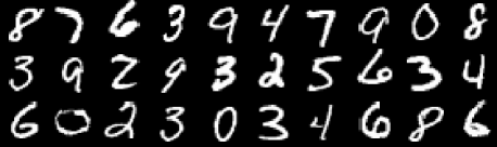
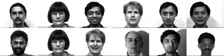
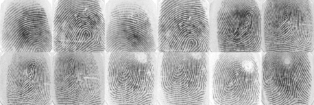
Figure 1: Examples for matrix datasets. a MNIST samples. b Yale face samples. c FingerDB samples

One-to-one classification method is introduced when it comes to multiple classification problem. All data are standardized into $[0,1]$ through linear transformation. The input matrices are converted into vectors when it comes to the SVM problems. All kernels select the optimal trade-off parameter $C\in\{10^{-2},10^{-1},\ldots,10^{2}\}$, kernel width parameter $\sigma\in\{10^{-4},10^{-3},\ldots,10^{4}\}$ and rank $r\in\{1,2,\cdots,10\}$. All the learning machines use the same training and test set. For the purpose of parameter selection, grid search is introduced in experiments. In MRMLKSVM and new matrix kernel, Gaussian RBF kernel $k(\textbf{x},\textbf{y})=\exp(-\sigma\|\textbf{x}-\textbf{y}\|^{2})$ and polynomial kernel $k(\textbf{x},\textbf{y})=(\textbf{x}^{T}\textbf{y}+\sigma)^{2}$ are used respectively as the vector kernel functions. Gaussian RBF kernel is used in DuSK which denoted as $\rm DuSK_{RBF}$. In addition, linear and Gaussian-RBF kernel are introduced on SVM classifier which denoted as $\rm SVM_{linear}$ and $\rm SVM_{RBF}$ respectively.

To evaluate the performance of the different kernels, we introduce two performance measures. We report the accuracy which counts on the proportion of correct predictions, the $F_{1}$ score as the harmonic mean of precision and recall $F_{1}=2\cdot\frac{Pre\times Rec}{Pre+Rec}$. Precision is the fraction of retrieved instances that are relevant, while recall is the fraction of relevant instances that are retrieved. In multiple classification problems, macro-averaged F-measure (Yang and Liu, 1999) is adopted as the average of $F_{1}$ score for each category.

4.3 Discussions

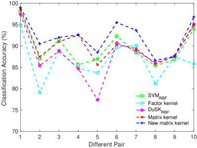
(a) 100 train

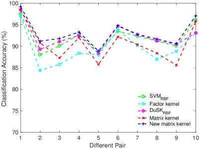
(b) 1000 train

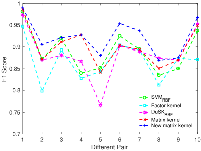
(c) 100 train

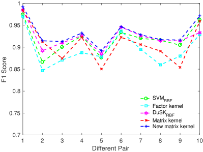
(d) 1000 train

Figure 2: Average accuracy and $F_{1}$ score compared by different kernels for binary classification problem on MNIST dataset.

Fig. 2 summarizes the results of $\rm SVM_{RBF}$, factor kernel, $\rm DuSK_{RBF}$, MRMLKSVM and new matrix kernel in terms of accuracy and $F_{1}$ score on MNIST dataset. The linear kernel-based SVM is not included because Gaussian-RBF kernel-based SVM proved to be better in the literature (Liu et al, 2003). Similar patterns of curves are detected in accuracy and $F_{1}$ score among all the kernel methods. We can observe that our new matrix kernel performs well in general which demonstrates the effectiveness of the proposed algorithm. We are interested in accuracy and $F_{1}$ score in kernel comparison experiments and one way to understand this is to realize that matrices are calculated to construct our new kernel which occupies much more space and time. On the other hand, MRMLKSVM is competitive against $\rm SVM_{RBF}$, factor kernel and $\rm DuSK_{RBF}$, performs worse than our new matrix kernel. In addition, the observations demonstrate the size of training set has positive effect on the performance in most cases.

Table 1: Prediction performance of different kernels on experimental datasets in terms of accuracy and macro-averaged F-measure

Kernel	Accuracy $(\%)$		F-measure
	Yale Face	FingerDB	Yale Face	FingerDB
$\rm SVM_{linear}$	86.9(3.7)	72.0(5.8)	0.871(0.036)	0.700(0.064)
$\rm SVM_{RBF}$	85.6(3.6)	73.0(4.0)	0.859(0.035)	0.712(0.045)
Factor Kernel	76.0(5.2)	64.0(2.5)	0.764(0.052)	0.599(0.043)
$\rm DuSK_{RBF}$	80.8(3.2)	73.5(2.5)	0.808(0.033)	0.732(0.033)
$\rm MRMLKSVM_{RBF}$	84.0(4.4)	72.5(2.7)	0.844(0.040)	0.719(0.029)
$\rm NewMatrixKernel_{poly}$	89.3(4.9)	75.0(3.5)	0.892(0.049)	0.741(0.036)

Table LABEL:Table1 reports the performance of several types of kernels with respect to accuracy and macro-averaged F-measure for multiple classification problems, where best results are highlighted in bold type. We can observe that both of accuracy and macro-averaged F-measure show the similar trend. Our new matrix kernel clearly benefits from its complexity and on both datasets it outperforms $\rm SVM_{linear}$, $\rm SVM_{RBF}$, $\rm DuSK_{RBF}$ and factor kernel in almost significant manner. Factor kernel performs significantly worse in all domains. On the other hand, MRMLKSVM performs slightly worse than our new matrix kernel and the performance of it is quite different on different data sets. This may due to the construction of the kernel where only the columns of matrix are under consideration, whereas information in the rows or inside the structure is lost.

Specifically, the learning algorithms which factorize the input matrices into the product of vectors tend to have a lower performance compared to those who preserve the initial structure. This indicates that approximation by decomposition would lose the compact structural information within data, leading to the diminished performance.

So far we have compared all experimental results. The results of classification accuracy and F-measure for $\rm DuSK_{RBF}$, factor kernel, SVM, MRMLKSVM and our new matrix kernel demonstrate that our new matrix kernel is significantly effective on both binary and multiple classification problems. Notice that we apply polynomial kernel in the construction of the new matrix kernel, and other types of vector kernel can also be adopted.

5 Concluding Remarks

In this paper we have established a mathematical framework of matrix Hilbert spaces. Intuitively, we introduce a matrix inner product to generalize the scalar inner product, which is especially useful in the presence of structured data. The reproducing kernel and the reproducing kernel matrix Hilbert space in our framework allow one to construct various structure of kernels in nonlinear cases. In our experiments, kernel induced by our framework has favourable predictive performance on both binary and multiple classification problems.

Matrix Hilbert space provides several interesting avenues for future work. For calculating the new matrix kernel developing computational methods could improve efficiency. Since the dimension of matrix inner product has a negative effect on the usage of space and time, we could pick up an appropriate one to balance the trade-off between efficiency and accuracy. While experiments have been conducted on the classification problems, our results indicate that RKMHS is directly applicable to regression, clustering, and ranking, among other tasks.