Direct CP asymmetry in $D\to\pi^{-}\pi^{+}$ and $D\to K^{-}K^{+}$ in QCD-based approach

Abstract

We present the first QCD-based calculation of hadronic matrix elements with penguin topology determining direct CP-violating asymmetries in $D^{0}\to\pi^{-}\pi^{+}$ and $D^{0}\to K^{-}K^{+}$ nonleptonic decays. The method is based on the QCD light-cone sum rules and does not rely on any model-inspired amplitude decomposition, instead leaning heavily on quark-hadron duality. We provide a Standard Model estimate of the direct CP-violating asymmetries in both pion and kaon modes and their difference and comment on further improvements of the presented computation.

I Introduction

Despite years of intense experimental efforts, CP-violation has never been unambiguously observed in the decays of up-type quarks. In the Standard Model (SM) this fact can be explained by the suppression of all CP-violating amplitudes resulting from the smallness of relevant Cabbibo-Kobayashi-Maskawa (CKM) matrix elements. To make matters worst, accurate predictions of up-type CP-violating observables are hard to obtain, since the necessary hadronic matrix elements are dominated by long-distance contributions. In order to calculate these matrix elements one needs to employ a QCD-based method that deals with nonperturbative effects in a model-independent manner. In this letter we shall calculate CP-violating observables in exclusive singly Cabibbo-suppressed (SCS) decays of $D$-mesons using a variant of light-cone QCD sum rules (LCSRs).

Observables that are sensitive to $CP$-violation are most often written in terms of asymmetries BigiSandaBook ,

$$a_{\rm CP}(f)=\frac{\Gamma(D\to f)-\Gamma(\overline{D}\to\overline{f})}{\Gamma(D\to f)+\Gamma(\overline{D}\to\overline{f})},$$ (1)

formed from the partial rates of a $D$-meson decay to a final state $f$ and of its CP-conjugated counterpart. Depending on the initial state, the asymmetry in Eq. (1) could be a function of time, if $D^{0}\,\overline{\!D}{}{}^{0}$-mixing is taken into account.

The measured time-integrated asymmetry contains a direct component (see, e.g., CPdirect ), which will be the main focus of this paper. Direct $CP$ asymmetry occurs when the absolute values of the $D\to f$ decay amplitude, which we denote by $A_{f}\equiv A(D\to f)$, and of the corresponding CP-conjugated amplitude ${\overline{A}}_{\bar{f}}\equiv A(\overline{D}\to\overline{f})$ are different. This can be realized if the decay amplitude $A_{f}$ can be separated into at least two different parts,

$$A_{f}=A_{f}^{\rm(1)}e^{i\delta_{1}}e^{i\phi_{1}}+A_{f}^{\rm(2)}e^{i\delta_{2}}e^{i\phi_{2}},$$ (2)

where $\phi_{1}\neq\phi_{2}$ are the weak phases (odd under $CP$), and $\delta_{1}\neq\delta_{2}$ are the strong phases (even under $CP$). The CP-violating asymmetry is then given by

$$a_{\rm CP}^{\rm dir}(f)\propto\frac{A_{f}^{\rm(1)}}{A_{f}^{\rm(2)}}\ \sin(\delta_{1}-\delta_{2})\sin(\phi_{1}-\phi_{2}).$$ (3)

The amplitude pattern of Eq. (2) naturally emerges in the SCS nonleptonic decays such as $D^{0}\to K^{-}K^{+}$ and $D^{0}\to\pi^{-}\pi^{+}$.

A model-independent computation of the amplitude ratio and the strong phase difference in Eq. (3) is a daunting task in charm physics (for reviews see e.g.,CPreview ). In SM, the sizes of direct CP-violating asymmetries for any final state are always proportional to a small combination of the CKM factors $V_{cb}^{*}V_{ub}$, which ensures that $a_{\rm CP}^{\rm dir}(f)$ is small even if the maximal strong phase difference is assumed. Hence, if a larger value of CP-violating asymmetry is observed, it would provide a “smoking gun” signal of new physics in the charm sector of quark-flavor transitions. However, due to a very uncertain hadronic input, the available estimates of $a_{\rm CP}^{\rm dir}(f)$ obtained with various degree of model dependence are mostly qualitative, predicting this asymmetry in the ballpark of a per mille.

Direct and indirect components of $CP$-violating asymmetries in the decays of neutral $D$-mesons can be separated with a careful time-dependent analysis. Since the indirect components to a large extent are independent of the final state, it is advantageous to consider differences of direct CP-violating asymmetries $\Delta a_{\rm CP}^{\rm dir}$,

$$\Delta a_{\rm CP}^{\rm dir}=a_{\rm CP}^{\rm dir}(f_{1})-a_{\rm CP}^{\rm dir}(f_{2}).$$ (4)

This difference is especially interesting if $CP$ asymmetries in the subtracted amplitudes are predicted to have opposite signs. This is in fact realized in SM for $f_{1}=K^{-}K^{+}$ and $f_{2}=\pi^{-}\pi^{+}$ final states.

Earlier experimental results seemed to indicate a somewhat large asymmetry (4) for these final states, with values reaching the order of $-1.0\%$. If confirmed, this would have indicated a possible new physics contribution to flavor-changing neutral currents (FCNC) in charm sector NP_predictions or a previously unaccounted SM contributions SM_predictions .

Current measurements, however, yield significantly lower values, with an average PDG

$$\Delta a^{dir}_{CP}=(-0.12\pm 0.13)\%\,,$$ (5)

including the most accurate measurement to date by LHCb collaboration using the $D^{*}$ tag Aaij:2016cfh ,

$$\Delta a^{dir}_{CP}=(-0.10\pm 0.08\pm 0.03)\%\,$$ (6)

in a qualitative agreement with the SM expectations NewSM_predictions .

Combination of indirect and direct CP-asymmetries for $K^{-}K^{+}$ and $\pi^{-}\pi^{+}$ final states have also been separately measured. Averaged over several experiments they are reported to be Amhis:2016xyh

$$a_{CP}(K^{-}K^{+})=(-0.16\pm 0.12)\%\,,~{}~{}a_{CP}(\pi^{-}\pi^{+})=(+0.00\pm 0.15)\%\,,$$ (7)

while the most recent combinations of measurements by LHCb collaboration read Aaij:2016dfb

$$a_{CP}(K^{-}K^{+}) = (0.04\pm 0.12\ (\mbox{stat})\pm 0.10\ (\mbox{syst}))\%\,,$$

$$a_{CP}(\pi^{-}\pi^{+}) = (0.07\pm 0.14\ (\mbox{stat})\pm 0.11\ (\mbox{syst}))\%\,.$$ (8)

Both asymmetries imply a very small effect, consistent with zero within current experimental uncertainties. Note again that in the SM opposite signs are expected for the asymmetries in the $K^{-}K^{+}$ and $\pi^{-}\pi^{+}$ channels.

New results with smaller experimental uncertainty are expected from the Run II LHCb data, as well as from the Belle II experiment. A model-independent calculation with controlled theoretical uncertainties of direct CP-violating asymmetries in SM is, therefore, compellingly needed. However, this task necessitates a calculation of hadronic matrix elements with strongly interacting and energetic two-meson final states, which is a big challenge even for the most advanced lattice QCD methods. In this situation even an order-of-magnitude QCD-based estimate of the hadronic input should become useful to reliably constrain the expected SM contribution to the CP-violating asymmetries.

The aim of this letter is to estimate the hadronic matrix elements relevant for the direct CP-violating asymmetries in $D^{0}\to P^{-}P^{+}$ decays ($P=\pi,K$), employing a computational method which combines the light-cone operator-product expansion (OPE) in QCD and hadronic dispersion relations. More specifically, we use the approach developed in AK01 for $B\to\pi\pi$ nonleptonic decays, in particular its application to the penguin-topology matrix elements KMM03 . We define matrix elements of “penguin topology” as those of the weak effective 4-quark operator containing a quark-antiquark pair not present in the valence-quark content of the final $P^{-}P^{+}$ state.

In what follows, we identify the hadronic matrix elements with penguin topologies which are needed to estimate the direct $CP$ asymmetry in $D^{0}\to\pi^{-}\pi^{+}$ and $D^{0}\to K^{-}K^{+}$ decays. We then briefly describe the method of Refs. AK01 ; KMM03 , adapting it to the $D^{0}\to P^{-}P^{+}$ decays. The main result is the QCD LCSR for the $D^{0}\to P^{-}P^{+}$ hadronic matrix elements with the penguin topology. The calculation, which takes into account $SU(3)_{F}$-violating ${\cal O}(m_{s})$ effects, is valid at large invariant mass $P^{2}$ of the $\pi^{-}\pi^{+}$ and/or $K^{-}K^{+}$ final state. Applying quark-hadron duality, the result is analytically continued to the physical point $P^{2}=m_{D}^{2}$. The rest of this letter contains numerical analysis and our estimate of the direct CP-asymmetry in $D^{0}\to P^{-}P^{+}$ decays, followed by a concluding discussion.

II $D^{0}\to\pi^{-}\pi^{+}$ and $D^{0}\to K^{-}K^{+}$ decay amplitudes

The singly Cabibbo suppressed decays of charmed mesons are driven by an effective Hamiltonian

$${\cal H}_{\rm eff}=\frac{G_{F}}{\sqrt{2}}\left[\sum_{q=d,s}\lambda_{q}\left(C_{1}{\cal Q}_{1}^{q}+C_{2}{\cal Q}_{2}^{q}\right)-\lambda_{b}\!\!\!\!\sum\limits_{i=3,...,6,8g}C_{i}{\cal Q}_{i}\right]\,,$$ (9)

where the products of CKM matrix elements $\lambda_{q}$ are defined as

$$\lambda_{q}=V_{uq}V^{*}_{cq},\quad\mbox{with}\ \ q=d,s,b\,.$$ (10)

Unitarity of the CKM matrix implies that

$$\sum_{q=d,s,b}\lambda_{q}=0\ \ \mbox{or}\ \ \lambda_{d}=-(\lambda_{s}+\lambda_{b}).$$ (11)

Since the goal of this paper is to capture the dominant contributions to the decay amplitudes in the SM, we shall only take into account the effective current-current operators,

$${\cal Q}_{1}^{q}=\left(\bar{u}\Gamma_{\mu}q\right)\left(\bar{q}\Gamma^{\mu}c\right),\quad\quad{\cal Q}_{2}^{q}=\left(\bar{q}\Gamma_{\mu}q\right)\left(\bar{u}\Gamma^{\mu}c\right)\,,$$ (12)

where $\Gamma_{\mu}=\gamma_{\mu}(1-\gamma_{5})$, and $q=d,s$. We shall neglect the penguin operators ${\cal Q}_{i=3,...,6,8g}$ with small Wilson coefficients.

Furthermore, we introduce a compact notation for the linear combination of the operators (12) with their Wilson coefficients and the Fermi constant,

$${\cal O}^{q}\equiv\frac{G_{F}}{\sqrt{2}}\sum\limits_{i=1,2}C_{i}{\cal Q}^{q}_{i}\,,\quad\ \mbox{with}\ \ q=d,s.$$ (13)

The dominant contribution to the two-body $D^{0}\to P^{-}P^{+}$ nonleptonic decay amplitudes is given by the hadronic matrix elements of ${\cal O}^{q}$,

$$A(D^{0}\to\pi^{-}\pi^{+}) = \lambda_{d}\langle\pi^{-}\pi^{+}|{\cal O}^{d}|D^{0}\rangle+\lambda_{s}\langle\pi^{-}\pi^{+}|{\cal O}^{s}|D^{0}\rangle\,,$$ (14)

$$A(D^{0}\to K^{-}K^{+}) = \lambda_{s}\langle K^{-}K^{+}|{\cal O}^{s}|D^{0}\rangle+\lambda_{d}\langle K^{-}K^{+}|{\cal O}^{d}|D^{0}\rangle\,.$$ (15)

Applying the CKM unitarity relation of Eq. (11) to Eqs. (14) and (15), and subsequently adding and subtracting a term $\lambda_{b}\ \langle\pi^{-}\pi^{+}|{\cal O}^{s}|D^{0}\rangle$ to right-hand side of Eq. (14), we arrange the decay amplitudes in the following form,

$$A(D^{0}\to\pi^{-}\pi^{+}) = -\lambda_{s}{\cal A}_{\pi\pi}\left[1+\frac{\lambda_{b}}{\lambda_{s}}\left(1+r_{\pi}\exp(i\delta_{\pi})\right)\right],$$

$$A(D^{0}\to K^{-}K^{+}) = \phantom{-}\lambda_{s}{\cal A}_{KK}\left[1-\frac{\lambda_{b}}{\lambda_{s}}r_{K}\exp(i\delta_{K})\right],$$ (16)

where we introduce compact notations for the ratios

$$r_{\pi}=\left|\frac{{\cal P}_{\pi\pi}^{s}}{{\cal A}_{\pi\pi}}\right|\,,~{}~{}~{}~{}r_{K}=\left|\frac{{\cal P}_{KK}^{d}}{{\cal A}_{KK}}\right|$$ (17)

of hadronic matrix elements

$${\cal P}_{\pi\pi}^{s}=\langle\pi^{-}\pi^{+}|{\cal O}^{s}|D^{0}\rangle\,,~{}~{}~{}~{}{\cal P}_{KK}^{d}=\langle K^{-}K^{+}|{\cal O}^{d}|D^{0}\rangle\,,$$ (18)

and

$${\cal A}_{\pi\pi} = \langle\pi^{-}\pi^{+}|{\cal O}^{d}|D^{0}\rangle-\langle\pi^{-}\pi^{+}|{\cal O}^{s}|D^{0}\rangle\,,$$

$${\cal A}_{KK} = \langle K^{-}K^{+}|{\cal O}^{s}|D^{0}\rangle-\langle K^{-}K^{+}|{\cal O}^{d}|D^{0}\rangle\,,$$ (19)

and denote by $\delta_{\pi(K)}$ the difference between the strong phases of the amplitudes ${\cal P}_{\pi\pi(KK)}^{s(d)}$ and ${\cal A}_{\pi\pi(KK)}$. In what follows, we do not attempt to calculate the amplitudes ${\cal A}_{\pi\pi}$ and ${\cal A}_{KK}$, having in mind their complicated form in terms of hadronic matrix elements with various quark topologies. Instead, as follows from Eq. (16), these amplitudes can be extracted to a reasonable precision from the measured partial widths of $D^{0}\to\pi^{-}\pi^{+}$ and $D^{0}\to K^{-}K^{+}$ decays, neglecting small parts of the amplitudes proportional to $\lambda_{b}$.

It is instructive to discuss the flavor $SU(3)_{F}\,$-symmetry limit of the decay amplitudes in Eq. (16). In this limit separate hadronic matrix elements with pions and kaons in the final state are equal: ${\cal A}_{KK}={\cal A}_{\pi\pi}$, $r_{K}=r_{\pi}$ and $\delta_{K}=\delta_{\pi}$. Still, with $\lambda_{b}\neq 0$, the decay amplitudes in Eq. (16) differ from each other by $O(\lambda_{b})$ terms. This difference can be easily understood in the $U$-spin symmetry limit, in which the initial $D^{0}$-state is a $U$-singlet. The effective Hamiltonian of Eq. (9) transforms as a combination of a $U$-triplet and $U$-singlet, the latter being proportional to $\lambda_{b}$, so that there are two $U$-spin invariant amplitudes contributing to $A(D\to\pi^{-}\pi^{+})$ and $A(D\to K^{-}K^{+})$ with different coefficients .

The representation in Eq. (16) has the advantage that the parts of the amplitudes proportional to $\lambda_{b}/\lambda_{s}$ generate direct $CP$-violating asymmetries, due to the weak phase contained in this combination of CKM parameters. The asymmetries will vanish if either the ratio $r_{\pi,K}\to 0$ or the strong phase $\delta_{\pi,K}\to 0$. Hence, computation of the ratios $r_{\pi,K}$ and the phases $\delta_{\pi,K}$ will result in the prediction of direct CP-violating asymmetries of Eq. (4).

It is important to note that we will not be using the expansion of the decay amplitudes in flavor topology diagrams, which is frequently employed in the analysis of two-body nonleptonic decays of charmed meson, starting from the earlier papers quarkdiag (for a more recent analysis see, e.g, Rosner2010 ). In that approach, flavor symmetries and experimental data are used to fit the “topological amplitudes”. In our calculation, such expansion is unnecessary, first of all because we are only calculating the “penguin topology” matrix elements in Eq. (18), estimating the dominant part of the decay amplitudes from experimental measurements.

Most importantly, in the commonly adopted convention, since the part of decay amplitude containing weak phase is suppressed by a very small CKM coefficient $\lambda_{b}$, it is not feasible to extract this part from the experimentally observed decay rates, but rather calculate it directly, as it is done in this letter.

III Hadronic Matrix elements from LCSRs

Here we adapt for nonleptonic $D$-decays the approach to compute hadronic amplitudes for $B\to\pi\pi$ decays suggested in AK01 and based on the method of QCD LCSRs lcsr . In particular, we will readily use the calculation of hadronic matrix elements of $B\to\pi\pi$ decays with charm penguin topology performed in KMM03 . We start from the $D^{0}\to\pi^{-}\pi^{+}$ transition aiming at estimating the $s$-quark “penguin” contribution ${\cal P}_{\pi\pi}^{s}$ to this decay amplitude. Following KMM03 , the starting object is the correlation function

$$F_{\alpha}(p,q,k)=i^{2}\int d^{4}xe^{-i(p-q)x}\int d^{4}ye^{i(p-k)y}\langle 0|\ T\left\{j_{\alpha 5}^{(\pi)}(y){\cal Q}_{1}^{s}(0)j_{5}^{(D)}(x)\right\}|\pi^{+}(q)\rangle$$

$$=(p-k)_{\alpha}F((p-k)^{2},(p-q)^{2},P^{2})+\dots,$$ (20)

where $j_{\alpha 5}^{(\pi)}=\bar{d}\gamma_{\alpha}\gamma_{5}u$ and $j_{5}^{(D)}=im_{c}\bar{c}\gamma_{5}u$ are, respectively, the pion and $D$-meson interpolating currents, sandwiched together with the four-quark operator ${\cal Q}_{1}^{s}$ between the on-shell pion and vacuum state. The ellipsis denote the kinematical structures we do not use. Note that performing a Fierz transformation of the operator ${\cal Q}^{s}_{1}$, the combination of current-current operators entering the effective Hamiltonian of Eq. (9) is transformed:

$$C_{1}{\cal Q}_{1}^{s}+C_{2}{\cal Q}^{s}_{2}=2C_{1}\widetilde{{\cal Q}}_{2}^{s}+\left(\frac{C_{1}}{3}+C_{2}\right){\cal Q}^{s}_{2}\,,$$ (21)

so that the color-octet operator

$$\widetilde{{\cal Q}}_{2}^{s}=\left(\bar{s}\Gamma_{\mu}\frac{\lambda^{a}}{2}s\right)\left(\bar{u}\Gamma^{\mu}\frac{\lambda^{a}}{2}c\right)\,,$$ (22)

is the only one contributing to the penguin amplitude in the adopted approximation. Hence, we hereafter replace ${\cal Q}_{1}\to\widetilde{{\cal Q}}_{2}^{s}$ in the correlation function. The resulting hadronic matrix element obtained from LCSR below is related to the penguin matrix element:

$${\cal P}^{s}_{\pi\pi}=\frac{2G_{F}}{\sqrt{2}}\ C_{1}\langle\pi^{+}\pi^{-}|\widetilde{{\cal Q}}_{2}^{s}|D^{0}\rangle\,.$$ (23)

Following AK01 we introduce an auxiliary 4-momentum $k$ flowing from the vertex of the weak interaction in the correlation function (20) and assume $k^{2}=0$, and, for simplicity, $p^{2}=0$. We adopt massless $u$ and $d$ quarks and a massless pion ($q^{2}=0$) approximation, so that the invariant amplitude determining the correlation function depends on three invariant variables $(p-k)^{2}$, $(p-q)^{2}$ and $P^{2}=(p-q-k)^{2}$. In the spacelike region $|(p-k)^{2}|,|(p-q)^{2}|\gg\Lambda_{QCD}^{2}$, $|P^{2}|\gg\Lambda_{QCD}^{2}$ the light-cone OPE expressed in terms of pion distribution amplitudes (DAs) is used to calculate the invariant amplitude $F((p-k)^{2},(p-q)^{2},P^{2})$.

As in KMM03 , the essential OPE diagrams are the ones shown in Fig. 1. We remind the reader that these diagrams stem from the light-cone OPE of the correlation function. Each diagram contains a coefficient function (hard-scattering amplitude) calculated perturbatively and convoluted with the pion distribution amplitudes (DAs) of growing twist and multiplicity. Therefore, only the highly-virtual quark and gluon lines corresponding to near-light-cone separation (large spacelike momentum transfer) between the two external currents with momenta $p-q$ and $p-k$ are included explicitly. In particular, the $s$-quarks in the loops also have large virtualities. The small-virtuality quarks and gluons are by default included in the pion DAs. Hence, for example, the diagrams with gluons emitted from the s-quark loop and absorbed in the pion DA should not be included in OPE .

Here, as in KMM03 , we only keep the contributions of two-particle twist-2 and twist-3 DAs and neglect all contributions of multiparticle pion DAs, since they correspond to higher-twist contributions to OPE and are suppressed by powers of characteristic large scales with respect to the lowest-twist contributions. In particular, we neglect contributions of diagrams where low virtuality (“soft”) gluons are emitted from the virtual quarks and form quark-antiquark-gluon DAs of twist 3 and 4. On the other hand, following KMM03 we take into account the diagram (c) containing the factorizable four-quark component of the pion DA, expressed via two-particle DA and vacuum quark condensate density. In the case of heavy charm-quark loop in $B\to\pi\pi$-decays considered in KMM03 there is a second diagram of this type with the $\bar{d}d$-condensate. In our correlation function such a diagram would only have small-virtuality $s$-quarks which cannot be resolved from the four-quark DAs, hence, it is absent in the context of OPE (see also discussion in KMM03 ). Note that the s-quark pair in the correlation function, being generated from the V-A current, cannot itself form the $\bar{s}s$ condensate. Hence, the small virtuality s-quark pairs can only form “genuine” nonfactorizable four-particle pion DAs originating from the nonlocal matrix element $\langle 0|\bar{d}(y)\bar{s}(0)s(0)u(x)|\pi^{+}\rangle$ and described by the diagram (d). As mentioned above, we neglect these contributions.

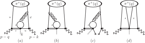
Figure 1: Diagrams contributing to the correlation function (20).

The expressions for the diagrams in Figs. 1(a)-(c) are then taken from KMM03 , replacing $b$-quark by $c$-quark and $c$-quark in the loop by $s$-quark. Derivation of LCSR follows then the same three-step procedure as the one developed and discussed in detail in AK01 and used in KMM03 . The first step is to use the hadronic dispersion relation for the invariant amplitude $F((p-k)^{2},(p-q)^{2},P^{2})$ in the variable $(p-k)^{2}=s$ of the pion channel, keeping the variables $(p-q)^{2}$ and $P^{2}$ fixed and spacelike, applying quark-hadron duality approximation in this channel with the effective threshold $s_{0}^{\pi}$ and performing the Borel transformation $(p-k)^{2}\to M_{1}^{2}$. The second step is the transition from spacelike to large timelike $P^{2}=m_{D}^{2}$, assuming local quark-hadron duality. At this stage we obtain the relation:

$$i\int d^{4}xe^{-i(p-q)x}\langle\pi^{-}(-q)\pi^{+}(p-k)|\ T\left\{{\cal Q}_{1}^{s}(0)j_{5}^{(D)}(x)\right\}|0\rangle$$

$$=\frac{-i}{\pi f_{\pi}}\int\limits_{0}^{s_{0}^{\pi}}dse^{-s/M_{1}^{2}}\mbox{Im}_{s}F(s,(p-q)^{2},m_{D}^{2})\,,$$ (24)

for the matrix element with two-pion final state, produced by the product of the operator ${\cal Q}_{1}^{s}$ and $D$-meson interpolating current with fixed $(p-q)^{2}<0$; $f_{\pi}$ in the above is the pion decay constant. The final third step is to apply to the above matrix element the hadronic dispersion relation in the variable $(p-q)^{2}=s^{\prime}$, combined with the quark-hadron duality approximation in the $D$-meson channel with the effective threshold $s_{0}^{D}$ and followed by the Borel transformation $(p-q)^{2}\to M_{2}^{2}$. After that the auxiliary 4-momentum $k$ vanishes for the $D$-meson pole term in the dispersion relation, leading to the sum rule for the $D^{0}\to\pi^{-}\pi^{+}$ hadronic matrix element:

$$\langle\!\pi^{-}\!(-q)\pi^{+}(p)|{\cal Q}_{1}^{s}|D^{0}(p-q)\rangle\!=\!\frac{-i}{\pi^{2}f_{\pi}f_{D}m_{D}^{2}}\!\!\int\limits_{0}^{s_{0}^{\pi}}\!\!ds\,\!e^{-s/M_{1}^{2}}\!\!\!\int\limits_{m_{c}^{2}}^{s_{0}^{D}}\!\!ds^{\prime}\,\!e^{(m_{D}^{2}-s^{\prime})/M_{2}^{2}}\mbox{Im}_{s^{\prime}}\mbox{Im}_{s}F(s,s^{\prime}\!,\!m_{D}^{2}),$$ (25)

where $f_{D}$ is the $D$-meson decay constant. The right-hand side of this expression is obtained by computing the double imaginary part of the sum of OPE diagrams, resulting in the final form of LCSR,

$$\langle\pi^{-}\pi^{+}|\widetilde{{\cal Q}}_{2}^{s}|D^{0}\rangle = i\frac{\alpha_{s}C_{F}m_{c}^{2}}{8\pi^{3}m_{D}^{2}f_{D}}\Bigg{[}\int\limits_{0}^{s_{0}^{\pi}}dse^{-s/M_{1}^{2}}\int\limits_{u_{0}^{D}}^{1}\frac{du}{u}e^{\left(m_{D}^{2}-\frac{m_{c}^{2}}{u}\right)/M_{2}^{2}}$$ (26)

$$\times \Bigg{\{}P^{2}\!\!\int\limits_{0}^{1}dzI(zuP^{2},m_{s}^{2})\Bigg{(}z(1-z)\varphi_{\pi}(u)$$

$$+ (1-z)\frac{\mu_{\pi}}{2m_{c}}\Big{[}\left(2z+\frac{m_{c}^{2}}{uP^{2}}\right)u\phi^{p}_{3\pi}(u)+\frac{1}{3}\left(2z-\frac{m_{c}^{2}}{uP^{2}}\right)\left(\phi^{\sigma}_{3\pi}(u)-\frac{u\phi^{\sigma^{\prime}}_{3\pi}(u)}{2}\right)\Big{]}\Bigg{)}$$

$$- \frac{\mu_{\pi}m_{c}}{4}\int\limits_{0}^{1}dzI(-z\bar{u}m_{c}^{2}/u,m_{s}^{2})\frac{\bar{u}^{2}}{u}\Big{[}\left(1+\frac{3m_{c}^{2}}{uP^{2}}\right)\phi^{p}_{3\pi}(1)+\left(1-\frac{5m_{c}^{2}}{uP^{2}}\right)\frac{\phi^{\sigma\prime}_{3\pi}(1)}{6}\Big{]}\Bigg{\}}$$

$$+ \frac{2\pi^{2}}{3}m_{c}(-\langle\bar{q}q\rangle)\int\limits_{u_{0}^{D}}^{1}\frac{du}{u^{2}}e^{\left(m_{D}^{2}-\frac{m_{c}^{2}}{u}\right)/M_{2}^{2}}\Bigg{\{}I(uP^{2},m_{s}^{2})\Bigg{(}2\varphi_{\pi}(u)+\frac{\mu_{\pi}}{m_{c}}\Big{[}3u\phi^{p}_{3\pi}(u)$$

$$+ \frac{\phi^{\sigma}_{3\pi}(u)}{3}-\frac{u\phi^{\sigma\prime}_{3\pi}(u)}{6}\Big{]}\Bigg{)}\Bigg{\}}\Bigg{]}_{P^{2}\to m_{D}^{2}}\,,$$

where $u_{0}^{D}=m_{c}^{2}/s_{0}^{D}$. The above expression is valid at large positive $P^{2}\gg s_{0}^{\pi}$, and the power corrections $O(s_{0}^{\pi}/P^{2})$ are neglected. In Eq. (26) the quark-loop function is defined KMM03 as

$$I(\ell^{2},m_{q}^{2})=\frac{1}{6}+\int\limits_{0}^{1}dxx(1-x)\ln\left[\frac{m_{q}^{2}-x(1-x)\ell^{2}}{\mu^{2}}\right]\,.$$ (27)

Note that the contributions from diagrams in Fig. 1a (Fig. 1b) are presented in the second and third (fourth) lines of Eq. (26), and the one from Fig. 1c occupies the fifth and sixth lines of Eq. (26). The pion DAs entering the LCSR are $\varphi_{\pi}(u)$ and $\varphi_{3p}^{\pi}(u),\varphi_{3p}^{\pi}(u)$, of twist-2 and twist-3, respectively. They depend, as usual, on the fraction of the longitudinal momentum of the pion $u$ ($\bar{u}=1-u$) carried by the quark (antiquark). We define $\phi^{\sigma\prime}_{3\pi}(u)=d\phi^{\sigma\prime}_{3\pi}(u)/du$ and adopt the truncated expansion in Gegenbauer polynomials $C_{n}^{(\alpha)}(u-\bar{u})$ for these DAs. We take

$$\varphi_{\pi}(u)=6u\bar{u}\left(1+a_{2}^{\pi}C^{3/2}_{2}(u-\bar{u})+a_{4}^{\pi}C^{3/2}_{4}(u-\bar{u})\right)\,,$$ (28)

for the twist-2 DA, and

$$\phi^{p}_{3\pi}(u) = 1+30\frac{f_{3\pi}}{\mu_{\pi}f_{\pi}}C_{2}^{1/2}(u-\bar{u})-3\frac{f_{3\pi}\omega_{3\pi}}{\mu_{\pi}f_{\pi}}C_{4}^{1/2}(u-\bar{u}),$$

$$\phi^{\sigma}_{3\pi}(u) = 6u(1-u)\left(1+5\frac{f_{3\pi}}{\mu_{\pi}f_{\pi}}\left(1-\frac{\omega_{3\pi}}{10}\right)C_{2}^{3/2}(u-\bar{u})\right)\,,$$ (29)

for the twist-3 DAs. Note that the Gegenbauer moments $a^{\pi}_{2,4}$ entering the twist-2 DA, the normalization parameter $\mu_{\pi}=m_{\pi}^{2}/(m_{u}+m_{d})$, and the parameters $f_{3\pi},\omega_{3\pi}$ of the non-asymptotic parts in twist-3 DAs represent nonperturbative inputs determined from various sources. Their scale dependence is not shown for brevity and taken into account at leading order (see e.g., KMMO for more details). In Eq. (26), $\langle\bar{q}q\rangle\equiv\langle 0|\bar{u}u|0\rangle$ is the quark-condensate density. Following other applications of QCD sum rules, we use the $\overline{MS}$ values for quark masses $m_{c}$ and $m_{s}$ in the numerical analysis.

Similar considerations hold for the calculation of $D$-decay to the kaon final state. For the kaon amplitude the analogous sum rule is obtained by replacing the following quantities in the correlation function of Eq. (20): $\bar{d}\to\bar{s}$ in the interpolating current (so that $j_{\alpha_{5}}^{(\pi)}\to j_{\alpha_{5}}^{(K)}$), the operator ${\cal Q}_{1}^{s}\to{\cal Q}_{1}^{d}$, and the final state $|\pi^{+}\rangle\to|K^{+}\rangle$. Correspondingly, the diagrams in Fig. 1 will change their flavor content, in particular, the $s$-quark loop will be replaced by the $d$-quark loop, which is easily taken into account by putting the mass of the internal quark in Eq. (27) to zero. In the rest of the diagrams we intend to include $O(m_{s})$ and, correspondingly, $O(m_{K}^{2})$ terms in order to assess the flavor $SU(3)_{F}$ violation in the hadronic matrix elements .

Summarizing, the LCSR for the hadronic matrix element $\langle K^{+}K^{-}|\widetilde{{\cal O}}_{2}^{d}|D^{0}\rangle$ is then obtained from Eq. (26) by the following replacements,

$$s_{0}^{\pi} \to s_{0}^{K}\,,~{}~{}e^{-s/M_{1}^{2}}\to e^{(m_{K}^{2}-s)/M_{1}^{2}}\,,$$

$$e^{\left(m_{D}^{2}-\frac{m_{c}^{2}}{u}\right)/M_{2}^{2}} \to e^{\left(m_{D}^{2}-\frac{m_{c}^{2}+m_{K}^{2}\bar{u}u}{u}\right)/M_{2}^{2}},~{}~{}I(..,m_{s}^{2})\to I(...,0)\,,~{}~{}$$ (30)

$$\varphi_{\pi}(u) \to \varphi_{K}(u),~{}~{}~{}~{}\varphi^{\pi}_{p}(u)\to\varphi^{K}_{p}(u)\,,~{}~{}\varphi^{\pi}_{\sigma}(u)\to\varphi^{K}_{\sigma}(u)\,,$$

as well as by replacing $\langle\bar{q}q\rangle\to\langle\bar{s}s\rangle$, $\mu_{\pi}\to\mu_{K}$ and $f_{\pi}\to f_{K}$. In the interest of succinctness we only quote the kaon DA of twist-2,

$$\varphi_{K}(u)=6u\bar{u}\left(1+a_{1}^{K}C^{3/2}_{1}(u-\bar{u})+a_{2}^{K}C^{3/2}_{2}(u-\bar{u})\right)\,,$$ (31)

where the Gegenbauer moment $a_{1}^{K}$ reflects the $SU(3)_{F}$-violating asymmetry of the $\bar{s}$ and $u$-quark average momentum fractions in the DA. The expressions for kaon twist-3 DAs can be found, e.g., in KMMO ; BBL . Apart from the parameters $\mu_{K}$, $f_{3K}$, $\omega_{3K}$, analogous to the pion ones in Eq. (29), these DAs also contain certain $O(m_{s})$ corrections and an additional $SU(3)_{F}$-asymmetry parameter $\lambda_{3K}$.

Note that here, similarly to the LCSR analysis of $B\to 2\pi$ decays KMM03 , we neglect the penguin-annihilation contribution, which is expected to be $\alpha_{s}$- and power-suppressed. In principle, this contribution can be separately estimated using the same approach. That evaluation is however technically more involved, as it contains multiloop contributions.

In conclusion of this section we emphasize that the pion and kaon DAs of the lowest twist, as well as the interpolating currents of pion, kaon and $D$-meson all have a valence quark content of the corresponding hadrons, whereas the hadronic matrix elements ${{\cal P}_{\pi\pi(KK)}^{s(d)}}$ are obtained from the diagrams where the quark pair in the relevant operator has a flavor different from the valence content. Hence, using the quark-hadron duality ansatz employed in the LCSRs, a hadronic matrix element with penguin topology is unambiguously identified, being “protected” at the level of correlation function from additional quark-antiquark insertions. Indeed, in the OPE such insertions in DAs or in interpolating currents would produce $\alpha_{s}$-suppressed and/or higher-twist (power suppressed) contributions.

IV Numerical results

In order to estimate the size of the computed hadronic matrix elements we need to provide numerical inputs for various parameters used in this calculation. We make conventional choices for the renormalization and factorization scale $\mu$ in LCSRs, adopting $\mu=1.5\pm 0.5$ GeV. The intervals of the (universal) Borel parameter $M_{1}^{2}=1.0\pm 0.5$ GeV² in the $\pi,K$ -meson channels, and the corresponding thresholds $s_{0}^{\pi}=0.7\pm 0.1$ GeV², $s_{0}^{K}=1.2\pm 0.1$ GeV² are inspired by the analysis of LCSRs for the pion and kaon electromagnetic form factors BKM . The corresponding parameters for $D$ meson channel, $M_{2}^{2}=4.5\pm 1.0$ GeV², $s_{0}^{D}=7.0\pm 0.5$ GeV² are taken following the LCSR analysis of $D\to\pi,K$ form factors KMMO . We display our choices for the remaining input parameters in Table 1. They include the strong coupling, quark masses, quark-condensate densities and the parameters of pion and kaon DAs, all rescaled to the adopted scale. Finally, we use the value of $f_{D}=201\pm 13$ MeV for the $D$-meson decay constant obtained from the 2-point QCD sum rule analysis in Gelhausen:2013wia , and the values $f_{\pi}=130.5$ MeV and $f_{K}=155.6$ MeV respectively PDG for the pion and kaon decay constants.

Parameter values	Parameter rescaled
and references	to $\mu=1.5$ GeV
$\alpha_{s}(m_{Z})=0.1181\pm 0.0011$  PDG	$0.351$
$\bar{m}_{c}(\bar{m}_{c})=1.27\pm 0.03$ GeV PDG	1.19 GeV
$\bar{m}_{s}(2\,\mbox{GeV})=96^{+8}_{-4}$ MeV  PDG	105 MeV
$\langle\bar{q}q\rangle(2\,\mbox{GeV})=(-276^{+12}_{-10}\,\mbox{MeV})^{3}$ PDG	$(-268\,\mbox{MeV})^{3}$
$\langle\bar{s}s\rangle=(0.8\pm 0.3)\langle\bar{q}q\rangle$  Ioffe:2002ee	$(-249~{}\mbox{MeV})^{3}$
$a_{2}^{\pi}(1\,\mbox{GeV})=0.17\pm 0.08$  Khodjamirian:2011ub	0.14
$a_{4}^{\pi}(1\,\mbox{GeV})=0.06\pm 0.10$  Khodjamirian:2011ub	0.045
$\mu_{\pi}(2\,\mbox{GeV})=2.48\pm 0.30$ GeV  PDG	2.26 GeV
$f_{3\pi}(1\,\mbox{GeV})=0.0045\pm 0.015$ GeV2  BBL	0.0036 GeV2
$\omega_{3\pi}(1\,\mbox{GeV})=-1.5\pm 0.7$  BBL	-1.1
$a_{1}^{K}(1\,\mbox{GeV})=0.10\pm 0.04$  Chetyrkin:2007vm	0.09
$a_{2}^{K}(1\,\mbox{GeV})=0.25\pm 0.15$  BBL	0.21
$\mu_{K}(2\,\mbox{GeV})=2.47^{+0.19}_{-0.10}$ GeV  PDG	2.25
$f_{3K}=f_{3\pi}$	0.0036 GeV2
$\omega_{3K}(1\,\mbox{GeV})=-1.2\pm 0.7$ BBL	-0.99
$\lambda_{3K}(1\,\mbox{GeV})=1.6\pm 0.4$  BBL	1.5

Table 1: The input parameters used in the numerical analysis of LCSRs and their values at the renormalization scale $\mu=1.5$ GeV.

With the chosen input, the results for the hadronic matrix elements calculated from the sum rule in Eq. (26) and from its analogue for the kaon channel are

$$\langle~{}\pi^{+}\pi^{-}|\widetilde{\cal Q}_{2}^{s}|D^{0}\rangle = (9.50\pm 1.13)\times 10^{-3}\exp[i(-97.5^{\scriptstyle o}\pm 11.6)]\,\mbox{GeV}^{3}\,,$$

$$\langle K^{+}K^{-}|\widetilde{\cal Q}_{2}^{d}|D^{0}\rangle = (13.9\pm 2.70)\times 10^{-3}\exp[i(-71.6^{\scriptstyle o}\pm 29.5)]\,\mbox{GeV}^{3}\,,$$ (32)

where the imaginary parts generated by the quark loops should, in the quark-hadron duality approximation, reproduce the strong phases of these amplitudes .

Using Eq. (23), we employ the value for the Wilson coefficient $C_{1}(\mu=1.5\mbox{ GeV})=1.25$ calculated at the same characteristic scale as the one used in LCSR for the hadronic matrix element. Finally, we obtain the estimate of the dimensionless penguin amplitudes,

$$|{\cal P}_{\pi\pi}^{s}|=(1.96\pm 0.23)\times 10^{-7}\,,$$ (33)

$$|{\cal P}_{KK}^{d}|=(2.86\pm 0.56)\times 10^{-7}\,,$$ (34)

for the pion and kaon final states, respectively. The uncertainties in Eqs. (32), (33), and (34) are obtained by randomly varying input parameters (given above and in Table 1) within their adopted ranges interpreted as $1\sigma$-intervals. To this end, a statistics of $10^{4}$ parameter combinations was generated for each LCSR. We assume no correlation between various inputs which certainly makes the uncertainty estimate more conservative. One has to emphasize that only parametrical uncertainties are taken into account here. The approximation for the OPE diagrams we used from KMM03 neglects small terms of $O(s^{\pi}_{0}/m_{B}^{2})\sim 4\%$, hence additional corrections to the LCSRs at the level of $O(s^{\pi,K}_{0}/m_{D}^{2})\sim 30\%$ cannot be excluded in the case of $D$-meson hadronic matrix elements. A dedicated calculation of the OPE diagrams is needed to include these corrections.

The values in Eqs. (33) and (34) will be used in the next section to estimate the direct CP-violating asymmetries and their difference in kaon and pion channels.

V Direct CP-violating asymmetry

Neglecting $D^{0}\,\overline{\!D}{}{}^{0}$ mixing, the partial rates

$$\Gamma(f)\equiv\Gamma(D^{0}\to P^{-}P^{+})$$ (35)

for $P=\pi,K$ can be written as

$$\Gamma(D^{0}\to P^{-}P^{+})=\frac{p^{*}_{P}}{8\pi m_{D}^{2}}|A(D^{0}\to P^{-}P^{+})|^{2}\,,$$ (36)

where $p^{*}_{P}$ is the decay 3-momentum in the $D$-meson rest frame. In terms of the amplitude parametrization in Eq. (16), the direct part of the CP-asymmetry for the decay of a D-meson into kaons is

$$a_{CP}^{dir}(K^{-}K^{+})=-\frac{2r_{b}r_{K}\sin\delta_{K}\sin\gamma}{1-2r_{b}r_{K}\cos\gamma\cos\delta_{K}+r_{b}^{2}r_{K}^{2}}\,,$$ (37)

while the same asymmetry for the decay of a $D$-meson into pions is

$$a_{CP}^{dir}(\pi^{-}\pi^{+})=\frac{2r_{b}r_{\pi}\sin\delta_{\pi}\sin\gamma}{1+2r_{b}\cos\gamma(1+r_{\pi}\cos\delta_{\pi})+r_{b}^{2}(1+2r_{\pi}\cos\delta_{\pi}+r_{\pi}^{2})}\,.$$ (38)

In Eqs. (37) and (38) it was convenient to represent the ratio of CKM parameters as

$$\frac{\lambda_{b}}{\lambda_{s}}\equiv r_{b}e^{-i\gamma},~{}~{}$$ (39)

where, in terms of Wolfenstein parameters, the modulus is

$$r_{b}\equiv\left|\frac{V_{ub}V_{cb}^{*}}{V_{us}V_{cs}^{*}}\right|=A^{2}\lambda^{4}\sqrt{\rho^{2}+\eta^{2}}+O(\lambda^{6})\,.$$ (40)

while the phase $\gamma=\arg(\rho+i\eta)$ coincides with the angle $\gamma$ of the unitarity triangle.

Due to the interplay of CKM coefficients in SM, the individual direct $CP$-violating asymmetries $a_{CP}^{dir}(K^{-}K^{+})$ and $a_{CP}^{dir}(\pi^{-}\pi^{+})$ have opposite signs, as expected. Taking the difference of Eqs. (37) and (38), expanding the result in $r_{b}$, and keeping only the linear piece we obtain

$$\Delta a_{CP}^{dir}=a_{CP}^{dir}(K^{-}K^{+})-a_{CP}^{dir}(\pi^{-}\pi^{+})=-2r_{b}\sin\gamma(r_{K}\sin\delta_{K}+r_{\pi}\sin\delta_{\pi})+{\cal O}(r_{b}^{2})\,.$$ (41)

In order to perform a numerical analysis of the above formula we take the central values of the Wolfenstein parameters obtained from a global fit to the available (mainly $B$-physics) data PDG , $\lambda=0.22506$, $A=0.811$, $\rho=0.12714$ and $\eta=0.365016$, yielding $\gamma=70.8^{\scriptstyle o}$, so that $r_{b}\,\sin\gamma\simeq 0.633\times 10^{-3}$ .

Before using our results it is instructive to estimate the combination of hadronic parameters entering Eq. (41). It can readily be extracted from the most accurate LHCb result for $\Delta a_{CP}^{dir}$ presented in Eq. (6). By substituting $r_{b}\,\sin\gamma$ into Eq. (41) and neglecting the corrections of $O(r_{b}^{2})$, we obtain the following interval for the penguin contribution parameters,

$$0.12\leq\left(r_{K}\,\sin\delta_{K}+r_{\pi}\,\sin\delta_{\pi}\right)\leq 1.46\,,$$ (42)

where we allowed for one standard deviation for the experimental data adding in quadrature the errors quoted in Eq. (6). We see that the combination of amplitudes extracted from experiment is quite uncertain. Still, within $1\sigma$-deviation, quite large values of the relative magnitudes of penguin effects are allowed, especially if the phases are small.

To predict the ratios $r_{K}$ and $r_{\pi}$ from our calculations we extract the amplitudes $\left|{\cal A}_{\pi\pi}\right|$ and $\left|{\cal A}_{KK}\right|$ relating them via Eq. (16) (in which we neglect the small $O(\lambda_{b})$ terms on the right-hand side) to the decay amplitudes. For determination of the latter, we use the experimentally measured branching fractions PDG ,

$${\cal B}(D^{0}\to\pi^{-}\pi^{+})=(1.407\pm 0.025)\times 10^{-3}\,,~{}~{}{\cal B}(D^{0}\to K^{-}K^{+})=(3.97\pm 0.07)\times 10^{-3}\,.$$ (43)

Inverting Eq. (36), and using the above values together with the lifetime $\tau_{D0}=0.4101$ ps, we obtain

$$\left|{\cal A}_{\pi\pi}\right| \simeq \lambda_{s}^{-1}\left|A(D\to\pi^{-}\pi^{+})\right|\ \ =(2.10\pm 0.02)\times 10^{-6}~{}\mbox{GeV}\,,$$

$$\left|{\cal A}_{KK}\right| \simeq \lambda_{s}^{-1}\left|A(D\to K^{-}K^{+})\right|=(3.80\pm 0.03)\times 10^{-6}~{}\mbox{GeV}\,.$$ (44)

Finally, we use the estimated penguin hadronic matrix elements in Eqs. (33) and (34) to predict the ratios:

$$r_{\pi}=\frac{|{\cal P}_{\pi\pi}^{s}|}{|{\cal A}_{\pi\pi}|}=0.093\pm 0.011\,,\qquad r_{K}=\frac{|{\cal P}_{KK}^{d}|}{|{\cal A}_{KK}|}=0.075\pm 0.015\,.$$ (45)

Note that predicting the relative phase $\delta_{\pi}$ or $\delta_{K}$ of the total amplitude vs. penguin contribution is a difficult task which is beyond the calculation performed here. Although we obtained a certain prediction for the phase of the penguin contribution, the phase of the main amplitude still remains obscure. One substantial complication is a possible influence of nearby light-quark scalar resonances on the strong phases (see, e.g. Falk:1999ts ). Those resonances, however, are known to be rather broad, overlapping in the energy region of the $D$-meson mass. This gives us confidence that quark-hadron duality ansatz provides a reasonable approximation to the final result.

Substituting our estimates for $r_{\pi}$ and $r_{K}$ in Eqs. (37), (38) and (41) taken to $O(r_{b})$ and allowing for arbitrary strong phases $\delta_{\pi,K}$, we obtain the upper bounds,

$$\left|a_{CP}^{dir}(\pi^{-}\pi^{+})\right|<0.012\pm 0.001\%,~{}~{}\left|a_{CP}^{dir}(K^{-}K^{+})\right|<0.009\pm 0.002\%.$$

$$\left|\Delta a_{CP}^{dir}\right|<0.020\pm 0.003\%\,.~{}~{}~{}~{}~{}~{}~{}~{}~{}~{}~{}~{}~{}~{}$$ (46)

Alternatively, assuming that the phases $\delta_{\pi}$ and $\delta_{K}$ are given by the phases of ${\cal P}_{\pi\pi}^{s}$ and ${\cal P}_{KK}^{d}$ calculated above and presented in Eq. (32), we obtain

$$a_{CP}^{dir}(\pi^{-}\pi^{+}) = -0.011\pm 0.001\%,$$

$$a_{CP}^{dir}(K^{-}K^{+}) = \phantom{-}0.009\pm 0.002\%.$$ (47)

$$\Delta a_{CP}^{dir} = \phantom{-}0.020\pm 0.003\%\,.$$

This is equivalent to assuming that the dominant parts of the decay amplitudes parametrized according to Eq. (16) as $\lambda_{s}{\cal A}_{\pi\pi}$ and $\lambda_{s}{\cal A}_{KK}$ both have a small phase relative, respectively, to ${\cal P}_{\pi\pi}^{s}$ and ${\cal P}_{KK}^{d}$. Such a situation is realized, for example, in a very simplified scenario when the decay amplitudes are dominated by the factorization ansatz. Yet, this might not be a very reliable approximation, as the decompositions (19) of ${\cal A}_{\pi\pi}$ and ${\cal A}_{KK}$ contain hadronic matrix elements with different topologies, including the penguin-topology ones.

Our predictions (V) and (V) are consistent with the experimental results quoted in Eqs. (5), (6), and (7). Note however, that the predicted upper bound on the SM contribution to $\Delta a_{CP}^{dir}$ is about factor of five smaller than the magnitude of the central value of the currently available experimental interval (6).

VI Conclusion

In this letter, we presented a new method to estimate the key hadronic matrix elements determining the direct CP asymmetries and their difference in $D^{0}\to K^{-}K^{+}$ and $D^{0}\to\pi^{-}\pi^{+}$ nonleptonic decays. The method is a variant of the QCD-based LCSR technique adopted from the computations of $B\to\pi\pi$ decay amplitudes. A nontrivial strong rescattering phase emerges in the calculated hadronic matrix elements. Our results do not rely on any flavor-symmetry and/or model-inspired amplitude decomposition. They do, however, rely heavily on the assumption of quark-hadron duality, which introduces a yet unaccounted systematic uncertainty.

An interesting question, directly related to the duality violation is the influence of intermediate scalar-isoscalar $f_{0}$ resonances on the decay amplitudes. One possibility to address this question is to modify our method in the following way. Instead of directly continuing the calculated correlation function to the physical point $P^{2}=m_{D}^{2}$, one can match the result to the hadronic dispersion relation in the variable $P^{2}$ at spacelike $P^{2}<0$, adopting a certain pattern of resonances in this dispersion relation. The hadronic matrix element is then obtained by setting $P^{2}=m_{D}^{2}$ in the fitted dispersion relation. This, more involved version of the LCSR method is postponed to a future study.

Our main results are the ratios (45) of the calculated “penguin topology” matrix elements to the total $D^{0}\to P^{-}P^{+}$ decay amplitudes, extracting the absolute values of the latter amplitudes from experimental data on $D^{0}$-decay rates to charged pions and kaons.

The upper bounds (V) and estimates (V) obtained here for the direct CP-asymmetry in both pion and kaon modes and their difference quantitatively assess the expected amount of direct CP violation in the charm sector of Standard Model. We believe that our results will become useful for the interpretation of current and future measurements of this elusive effect.

Acknowledgements

The work of A.K. is supported by DFG Research Unit FOR 1873 “Quark Flavour Physics and Effective Field Theories”, contract No KH205/2-2. A.A.P. is supported in part by the U.S. Department of Energy under contract DE-SC0007983. A.A.P. is a Comenius Guest Professor at the University of Siegen.

References

- (1) I. I. Bigi and A. I. Sanda, CP violation (Cambridge University Press, 2000).
- (2) Y. Grossman, A. L. Kagan and Y. Nir, Phys. Rev. D 75 (2007) 036008; A. L. Kagan and M. D. Sokoloff, Phys. Rev. D 80, 076008 (2009).
- (3) S. Bianco, F. L. Fabbri, D. Benson and I. Bigi, Riv. Nuovo Cim. 26N7 (2003) 1; G. Burdman and I. Shipsey, Ann. Rev. Nucl. Part. Sci. 53, 431 (2003); M. Artuso, B. Meadows and A. A. Petrov, Ann. Rev. Nucl. Part. Sci. 58 (2008) 249; X. Q. Li, X. Liu and Z. T. Wei, Front. Phys. China 4 (2009) 49; A. Ryd and A. A. Petrov, Rev. Mod. Phys. 84 (2012) 65.
- (4) G. Isidori, J. F. Kamenik, Z. Ligeti and G. Perez, Phys. Lett. B 711, 46 (2012); G. F. Giudice, G. Isidori and P. Paradisi, JHEP 1204, 060 (2012); W. Altmannshofer, R. Primulando, C. T. Yu and F. Yu, JHEP 1204, 049 (2012); G. Hiller, Y. Hochberg and Y. Nir, Phys. Rev. D 85, 116008 (2012).
- (5) M. Golden and B. Grinstein, Phys. Lett. B 222, 501 (1989); D. Pirtskhalava and P. Uttayarat, Phys. Lett. B 712, 81 (2012); B. Bhattacharya, M. Gronau and J. L. Rosner, Phys. Rev. D 85, 054014 (2012); J. Brod, A. L. Kagan and J. Zupan, Phys. Rev. D 86, 014023 (2012); T. Feldmann, S. Nandi and A. Soni, JHEP 1206 (2012) 007; J. Brod, Y. Grossman, A. L. Kagan and J. Zupan, JHEP 1210, 161 (2012); E. Franco, S. Mishima and L. Silvestrini, JHEP 1205, 140 (2012).
- (6) C. Patrignani et al. [Particle Data Group], Chin. Phys. C 40 (2016) no.10, 100001.
- (7) R. Aaij et al. [LHCb Collaboration], Phys. Rev. Lett. 116 (2016) no.19, 191601 .
- (8) H. Y. Cheng and C. W. Chiang, Phys. Rev. D 85, 034036 (2012) Erratum: [Phys. Rev. D 85, 079903 (2012)]; H. Y. Cheng and C. W. Chiang, Phys. Rev. D 86, 014014 (2012); H. n. Li, C. D. Lu and F. S. Yu, Phys. Rev. D 86, 036012 (2012); I. I. Bigi, A. Paul and S. Recksiegel, JHEP 1106, 089 (2011).
- (9) Y. Amhis et al., arXiv:1612.07233 [hep-ex].
- (10) R. Aaij et al. [LHCb Collaboration], Phys. Lett. B 767, 177 (2017).
- (11) A. Khodjamirian, Nucl. Phys. B 605 (2001) 558.
- (12) A. Khodjamirian, T. Mannel and B. Melic, Phys. Lett. B 571 (2003) 75.
- (13) J. Charles et al. [CKMfitter Group], Eur. Phys. J. C 41 (2005) no.1, 1.
- (14) G. Hiller, M. Jung and S. Schacht, Phys. Rev. D 87 (2013) no.1, 014024
- (15) N. Cabibbo and L. Maiani, Phys. Lett. B 73 (1978) 418 [Erratum-ibid. B 76 (1978) 663]; D. Fakirov and B. Stech, Nucl. Phys. B 133 (1978) 315; A. Khodjamirian, Yad. Fiz. 30 (1979) 824; L. L. Chau, Phys. Rept. 95, 1 (1983); L. L. Chau and H. Y. Cheng, Phys. Rev. Lett. 56, 1655 (1986); J. L. Rosner, Phys. Rev. D 60 (1999) 114026;
- (16) B. Bhattacharya and J. L. Rosner, Phys. Rev. D 81, 014026 (2010).
- (17) I. I. Balitsky, V. M. Braun and A. V. Kolesnichenko, Sov. J. Nucl. Phys. 44 (1986) 1028; Nucl. Phys. B 312 (1989) 509; V. L. Chernyak and I. R. Zhitnitsky, Nucl. Phys. B 345 (1990) 137.
- (18) A. Khodjamirian, C. Klein, T. Mannel and N. Offen, Phys. Rev. D 80, 114005 (2009)
- (19) P. Ball, V. M. Braun and A. Lenz, JHEP 0605 (2006) 004
- (20) V. M. Braun, A. Khodjamirian and M. Maul, Phys. Rev. D 61 (2000) 073004; J. Bijnens and A. Khodjamirian, Eur. Phys. J. C 26 (2002) 67.
- (21) B. L. Ioffe, Phys. Atom. Nucl. 66 (2003) 30 [hep-ph/0207191].
- (22) A. Khodjamirian, T. Mannel, N. Offen and Y.-M. Wang, Phys. Rev. D 83 (2011) 094031.
- (23) K. G. Chetyrkin, A. Khodjamirian and A. A. Pivovarov, Phys. Lett. B 661 (2008) 250.
- (24) P. Gelhausen, A. Khodjamirian, A. A. Pivovarov and D. Rosenthal, Phys. Rev. D 88 (2013) 014015 Erratum: [Phys. Rev. D 89 (2014) 099901] Erratum: [Phys. Rev. D 91 (2015) 099901].
- (25) M. Bander, D. Silverman and A. Soni, Phys. Rev. Lett. 43 (1979) 242.
- (26) M. Beneke, G. Buchalla, M. Neubert and C. T. Sachrajda, Nucl. Phys. B 606 (2001) 245.
- (27) A. F. Falk, Y. Nir and A. A. Petrov, JHEP 9912, 019 (1999); E. Golowich and A. A. Petrov, Phys. Lett. B 427, 172 (1998).