The role of the $S_{3}$ GUT leptoquark in flavor universality and collider searches

Abstract

We investigate the ability of the $S_{3}$ scalar leptoquark to address the recent hints of lepton universality violation in $B$ meson decays. The $S_{3}$ leptoquark with quantum numbers $(\overline{\bm{3}},\bm{3},1/3)$ naturally emerges in the context of an $SU(5)$ GUT model without any conflict with the stringent limits from observed nucleon stability. Scalar leptoquark $S_{3}$ with left-handed couplings to 2nd and 3rd generations of charged leptons and down-type quarks seems well-suited to address both $R_{K^{(*)}}$ and $R_{D^{(*)}}$. We quantify this suitability with numerical fits to a plethora of relevant flavor observables. The proposed $SU(5)$ model calls for a second leptoquark state, i.e., $\tilde{R}_{2}$ with quantum numbers $(\bm{3},\bm{2},1/6)$, if one is to generate gauge coupling unification and neutrino mass. We accordingly include it in our study to investigate $\tilde{R}_{2}$’s ability to offset adverse effects of $S_{3}$ and thus improve a quality of numerical fits. A global fit of the leptoquark Yukawa couplings shows that large couplings of light $S_{3}$ to $\tau$ leptons are preferred. We furthermore identify $B\to K^{(*)}\bar{\nu}\nu$ as the most sensitive channel to probe the preferred region of parameter space. Large couplings of $S_{3}$ to $\tau$ leptons are finally confronted with the experimental searches for $\tau$ final states at the Large Hadron Collider. These searches comprise a study of decay products of the leptoquark pair production, as well as, and more importantly, an analysis of the high-mass $\tau\tau$ final states.

1 Introduction

At low energies there are a few experimentally measured observables that exhibit deviation from the Standard Model (SM) predictions. Among them, the three $B$ meson anomalies, indicating possible lepton flavor universality (LFU) violation, particularly stand out.

One of these anomalies manifests itself in the ratios

$$R_{D^{(*)}}=\frac{\Gamma(B\to D^{(*)}\tau^{-}\bar{\nu})}{\Gamma(B\to D^{(*)}\ell^{-}\bar{\nu})}\,,$$ (1)

according to the experimental results in Refs. Lees:2012xj ; Lees:2013uzd ; Huschle:2015rga ; Adachi:2009qg ; Bozek:2010xy ; Aaij:2015yra ; Hirose:2016wfn . The result for $R_{D}$ appears to be $1.9\,\sigma$ larger than the SM prediction, i.e., $R_{D}^{\rm SM}=0.286\pm 0.012$, that is obtained by relying on the lattice QCD results for both the vector and the scalar form factors Becirevic:2016yqi (see also Ref. Bigi:2016mdz ). The experimentally established $R_{D^{\ast}}=0.304\pm 0.020$ has also been confirmed Aaij:2015yra ; Hirose:2016wfn ; Amhis:2016xyh , and it appears to be $\sim 3\,\sigma$ larger than predicted value $R_{D^{\ast}}^{\rm SM}=0.252\pm 0.003$ Fajfer:2012jt . The deviation from the SM prediction in the $R_{D}$–$R_{D^{*}}$ plane is at 3.9 $\sigma$ level Ligeti:2016npd ; Crivellin:2016ejn ; Amhis:2016xyh and it has accordingly attracted a lot of attention recently Altmannshofer:2017poe ; Alonso:2016oyd ; Crivellin:2014zpa ; Bhattacharya:2014wla ; Bhattacharya:2015ida ; Hati:2015awg ; Sakaki:2014sea ; Fajfer:2012jt .

The remaining two $B$ meson anomalies are related to the $b\to s\ell^{+}\ell^{-}$ transition. Namely, the LHCb experiment has found that there are slight discrepancies between the SM prediction and the experimental results for the angular observable known as $P_{5}^{\prime}$ in $B\to K^{\ast}\mu^{+}\mu^{-}$ process. In many approaches this disagreement has been attributed to new physics (NP), although the tension might be a result of the SM QCD effects (see e.g. Ref. Capdevila:2017ert and references therein). The second of the two $b\to s\ell^{+}\ell^{-}$ transition anomalies has been found in the ratio of the branching fractions,

$$\begin{split}R_{K}\equiv\frac{\mathcal{B}(B^{+}\to K^{+}\mu^{+}\mu^{-})_{q^{2}\in[1,6]\mathrm{\,GeV^{2}}}}{\mathcal{B}(B^{+}\to K^{+}e^{+}e^{-})_{q^{2}\in[1,6]\mathrm{\,GeV^{2}}}}&=0.745\pm^{0.090}_{0.074}\pm 0.036\leavevmode\nobreak\ \textrm{\cite[cite]{\@@bibref{Authors Phrase1YearPhrase2}{Aaij:2014ora}{\@@citephrase{(}}{\@@citephrase{)}}}},\\ R_{K^{*}}^{q^{2}\in[1.1,6]\mathrm{\,GeV}^{2}}\equiv\frac{\mathcal{B}(B^{0}\to K^{*0}\mu^{+}\mu^{-})_{q^{2}\in[1.1,6]\mathrm{\,GeV^{2}}}}{\mathcal{B}(B^{0}\to K^{*0}e^{+}e^{-})_{q^{2}\in[1.1,6]\mathrm{\,GeV^{2}}}}&=0.69^{+0.11}_{-0.07}\pm 0.05\leavevmode\nobreak\ \textrm{\cite[cite]{\@@bibref{Authors Phrase1YearPhrase2}{Aaij:2017vbb}{\@@citephrase{(}}{\@@citephrase{)}}}},\\ R_{K^{*}}^{q^{2}\in[0.045,1.1]\mathrm{\,GeV^{2}}}&=0.66^{+0.11}_{-0.07}\pm 0.03\leavevmode\nobreak\ \textrm{\cite[cite]{\@@bibref{Authors Phrase1YearPhrase2}{Aaij:2017vbb}{\@@citephrase{(}}{\@@citephrase{)}}}}.\end{split}$$ (2)

The values the LHCb experiment measured for these ratios are consistently lower than the SM prediction, i.e., $R_{K}^{\mathrm{SM}}=1.00\pm 0.03$, in which the next-to-next-to-leading QCD corrections and soft QED effects have been included Bordone:2016gaq ; Hiller:2003js (for $R_{K^{*}}$ see Table 1 and references in Aaij:2017vbb ). In other words, the LHCb results point towards a significant effect of the lepton flavor universality violation in this process. Recently, Belle Collaboration Wehle:2016yoi found out that the angular observable $P_{5}^{\prime}$ agrees with the SM prediction much better for electrons than for muons. This important result suggests that it is much more likely that beyond the SM effects are present in the second generation of leptons, and that there are currently no effects in $b\to se^{+}e^{-}$ which would not be accounted for in the SM.

Many scenarios of NP Altmannshofer:2014cfa ; Becirevic:2016yqi ; Datta:2013kja ; Hiller:2014yaa ; Crivellin:2014zpa ; Glashow:2014iga ; Bhattacharya:2014wla ; Gripaios:2014tna ; Greljo:2015mma ; Ghosh:2014awa ; Crivellin:2015mga ; Crivellin:2015lwa ; Crivellin:2017zlb ; Sierra:2015fma ; Varzielas:2015iva ; Crivellin:2015era ; Celis:2015ara ; Freytsis:2015qca ; Fajfer:2015ycq ; Cox:2016epl ; Becirevic:2017jtw ; Kamenik:2017tnu ; Arnan:2017lxi ; Ghosh:2017ber ; Bardhan:2016uhr ; Capdevila:2017bsm have been investigated in order to explain either $R_{K^{(*)}}$ and $P_{5}^{\prime}$, or $R_{D^{(*)}}$ anomalies. An interesting observation was found in Ref. Bhattacharya:2014wla that $R_{K^{(*)}}$ and $P_{5}^{\prime}$ can be explained if NP couples only to the third generation of quarks and leptons. Furthermore, the authors of Refs. Calibbi:2015kma ; Greljo:2015mma noticed that both $R_{D^{(*)}}$ and $R_{K^{(*)}}$ puzzles can be correlated if the effective four-fermion semileptonic operators consist of left-handed doublets.

In this work we consider a Grand Unified Theory (GUT) inspired setting with a light scalar $S_{3}$ leptoquark (LQ) that transforms as $(\overline{\bm{3}},\bm{3},1/3)$ under the SM gauge group $SU(3)\times SU(2)\times U(1)$. The state $S_{3}$ is rendered baryon number conserving due to the GUT symmetry, as we discuss in Sec. 7, and generates purely left-handed current $\bar{L}L\bar{Q}Q$ operators which seem to be well-suited to explain the LFU puzzles if the $S_{3}$ mass is at the TeV scale. The need for the second light LQ state, $\tilde{R}_{2}$ in representation $(\bm{3},\bm{2},1/6)$, emerges naturally from the requirement of neutrino masses generation in the advocated GUT model as well as from the gauge coupling unification. We accordingly include $\tilde{R}_{2}$ in our study and investigate whether it could partially compensate for the adverse low-energy effects of $S_{3}$. In Sec. 2 we introduce relevant couplings of these two LQs with the SM fermions. We proceed to show how $S_{3}$ could, in principle, address the LFU puzzles in Sec. 3. We then present relevant additional constraints on the LQ parameters in Sec. 4. The low-energy flavor analysis is concluded in Sec. 5 with the global fit of the relevant couplings of the two LQs with quark-lepton pairs for three specific Yukawa structures. Sec. 6 is devoted to collider study of the model signatures in the LQ resonant pair production and in a $t$-channel LQ exchange contributing to $\tau\tau$ final states at LHC. We elaborate on the GUT construction behind the two LQ states in Sec. 7. Finally, we conclude in Sec. 8.

2 Model setup

The LQ multiplet $S_{3}(\overline{\bm{3}},\bm{3},1/3)$ interacts with the SM fermions in accordance with its quantum numbers, given in the brackets. The three charge eigenstate components of $S_{3}$, i.e., $S^{4/3}_{3}$, $S^{1/3}_{3}$, and $S^{-2/3}_{3}$, have the following Yukawa interactions with fermions Dorsner:2016wpm

$$\begin{split}\mathcal{L}_{S_{3}}=&-y_{ij}\bar{d}_{L}^{C\,i}\nu_{L}^{j}S^{1/3}_{3}-\sqrt{2}y_{ij}\bar{d}_{L}^{C\,i}e_{L}^{j}S^{4/3}_{3}+\\ &+\sqrt{2}(V^{*}y)_{ij}\bar{u}_{L}^{C\,i}\nu_{L}^{j}S^{-2/3}_{3}-(V^{*}y)_{ij}\bar{u}_{L}^{C\,i}e_{L}^{j}S^{1/3}_{3}+\mathrm{h.c.},\end{split}$$ (3)

where $V$ is the Cabibbo-Kobayashi-Maskawa (CKM) mixing matrix. Note that $S_{3}$ has purely left-handed couplings. The diquark interactions with $S_{3}$ are not shown in Eq. (3) since we assume that $S_{3}$ and its interactions originate from the GUT construction presented in Ref. Dorsner:2017wwn where the baryon number violating diquark couplings are forbidden due to the grand unified symmetry. The main goal of our study is to address the puzzles observed in neutral current LFU tests in the $R_{K}$ ratio (and related anomalies in $b\to s\mu^{+}\mu^{-}$) as well as in charged-current LFU ratios $R_{D^{(*)}}$. Thus we have clear target observables that we can affect with a small number of LQ Yukawa couplings.

In the context of SM complemented with effective operators (SM-EFT) it has been shown that NP models contributing to dimension-6 operators made out of left-handed quark and lepton doublets can explain both neutral- and charged-current LFU anomalies Bhattacharya:2014wla ; Alonso:2015sja ; Calibbi:2015kma ; Greljo:2015mma ; Feruglio:2017rjo . However, in an explicit NP model these effective interactions could be correlated, unlike in the effective theory, with other observables. Our intention is to quantify this correlation within this particular model.

The LQ state $S_{3}$ can affect all the target LFU observables with a minimal set of parameters, e.g., $y_{s\mu}$, $y_{b\mu}$, and $y_{b\tau}$. In this work, however, we also study the effect of the coupling $y_{s\tau}$ which enables a handle on the semitauonic modes entering $R_{D^{(*)}}$. The couplings of $S_{3}$ to $d_{L}$ and $e_{L}$ have to be rather small in order to avoid pressing bounds from LFV and kaon physics. We opt to set those couplings to zero to obtain the following flavor structure:

$$y=\begin{pmatrix}0&0&0\\ 0&y_{s\mu}&y_{s\tau}\\ 0&y_{b\mu}&y_{b\tau}\end{pmatrix},\qquad{V^{*}}y=\begin{pmatrix}0&V_{us}^{*}y_{s\mu}+V_{ub}^{*}y_{b\mu}&V_{us}^{*}y_{s\tau}+V_{ub}^{*}y_{b\tau}\\ 0&V_{cs}^{*}y_{s\mu}+V_{cb}^{*}y_{b\mu}&V_{cs}^{*}y_{s\tau}+V_{cb}^{*}y_{b\tau}\\ 0&V_{ts}^{*}y_{s\mu}+V_{tb}^{*}y_{b\mu}&V_{ts}^{*}y_{s\tau}+V_{tb}^{*}y_{b\tau}\end{pmatrix}.$$ (4)

Note that the Yukawa couplings of $S_{3}$ to up-type quarks are spread over generations due to CKM rotation. In what follows all Yukawa couplings are assumed to be real. The ansatz of Eq. (4) summarizes the most general $S_{3}$ scenario studied within our work, although we will also comment on more restricted scenarios, where some additional elements of $y$ will be set to zero.

Having only one LQ with mass around the $1\mathrm{\,TeV}$ scale would invalidate unification of gauge couplings, thus a second LQ state — $\tilde{R}_{2}$ in our case — is needed. The two electric charge eigenstates of $\tilde{R}_{2}$ couple only to down-type quarks:

$$\begin{split}\mathcal{L}_{\tilde{R}_{2}}=&-\tilde{y}_{ij}\bar{d}_{R}^{i}e_{L}^{j}\tilde{R}_{2}^{2/3}+\tilde{y}_{ij}\bar{d}_{R}^{i}\nu_{L}^{j}\tilde{R}_{2}^{-1/3}+\textrm{h.c.}.\end{split}$$ (5)

The doublet $\tilde{R}_{2}$ can accomodate the measured value of $R_{K}$, but its right-handed current contributions cause tensions with the reported value for $R_{K^{*}}$. In the current setting with strictly left-handed neutrinos $\tilde{R}_{2}$ does not interact with up-type quarks and thus cannot affect $R_{D^{(*)}}$. In our approach it is $S_{3}$ that could, in principle, address both LFU anomalies, whereas its side-effects in other well-constrained observables (e.g. $B_{s}$–$\bar{B}_{s}$ mixing and $B\to K^{(*)}\bar{\nu}\nu$) might be, hopefully, cancelled by $\tilde{R}_{2}$. Since $S_{3}$ will have largest effects in the $\tau$ sector we have to introduce couplings of $\tilde{R}_{2}$ to $\tau$ in order to compensate for potentially unwanted effects. In the following analysis we will analyze a light $S_{3}$ scenario with the couplings texture (4) and along with it test the viability of having light $\tilde{R}_{2}$ with nonzero Yukawas involving the $\tau$ lepton. Namely, we take

$$\tilde{y}=\begin{pmatrix}0&0&0\\ 0&0&\tilde{y}_{s\tau}\\ 0&0&\tilde{y}_{b\tau}\end{pmatrix}.$$ (6)

The mass of $\tilde{R}_{2}$ should be at around $1$ TeV in order to affect low-energy phenomenology, if required at all. We consistently take this to be the case when we discuss the role of $\tilde{R}_{2}$ in gauge coupling unification and the neutrino mass generation.

For both LQ states the rotations with the CKM matrix $V$, left over from the transition to the mass basis of fermions, have been assigned to the $u_{L}$ fields. For the study of flavor phenomenology the neutrinos can be safely considered as massless. Thus, Lagrangians in Eqs. (3) and (5) are written in the fermion mass basis with the exception of $\nu_{L}$ whose mass basis is ill-defined. We use flavor basis for the neutrinos, such that the Pontecorvo-Maki-Nakagawa-Sakata (PMNS) matrix becomes unity.

3 LFU violating contributions

In this section we focus on how the two light LQs would affect the LFU violating anomalies measured in $B$ meson decays. The gross features required of Yukawa matrices will be presented. The detailed discussion of additional observables and their interplay with the LFU anomalies will be presented in the next section.

3.1 Charged currents LFU: $R_{D^{(*)}}$

The largest LFU violating effect is in the charged current observables $R_{D^{(*)}}$. For a NP-induced effective operator that follows the chirality structure of the SM it has been shown that the dimensionless coupling of $\sim 0.1$ is needed, if new particles have mass of $\Lambda=1\mathrm{\,TeV}$ and contribute at tree level Freytsis:2015qca . The matched contributions of $S_{3}$ generate left-handed current operator, whereas $\tilde{R}_{2}$ cannot contribute to charged currents in this setup. In particular in $b\to c\ell\bar{\nu}$ transition the $S_{3}$ presence leads to the modification of the left-handed charged-current operators:

$$\mathcal{L}_{\mathrm{SL}}=-\frac{4G_{F}}{\sqrt{2}}\Bigg{[}(V_{UD}+g^{L}_{UD;\ell\ell})(\bar{U}\gamma^{\mu}P_{L}D)(\bar{\ell}\gamma_{\mu}P_{L}\nu_{\ell})\Bigg{]},\qquad U=u,c,t,\quad D=s,b,\quad\ell=\mu,\tau,$$ (7)

where the LQ term in Eq. (7) reads

$$g_{UD;\ell\nu}^{L}=-\frac{v^{2}}{4m_{S_{3}}^{2}}(Vy^{*})_{U\ell}y_{D\nu}.$$ (8)

The effect of $S_{3}$ may be also understood as nonuniversal CKM elements in semileptonic charged-current processes:

$$|V_{ij}^{(\ell)}|^{2}=|V_{ij}|^{2}\left[1-\frac{v^{2}}{2m_{S_{3}}^{2}}\mathrm{Re}\left(\frac{V_{is}}{V_{ij}}y_{s\ell}^{*}y_{j\ell}+\frac{V_{ib}}{V_{ij}}y_{b\ell}^{*}y_{j\ell}\right)\right],\qquad i=u,c,t,\quad j=s,b,\quad\ell=\mu,\tau.$$ (9)

One also has lepton flavor violating $S_{3}$ contributions parameterized by $g_{UD;\ell\nu}$, with their effect being much smaller since they do not interfere with the SM amplitude. They contribute at subleading order, namely at $v^{4}/m_{S_{3}}^{4}$ that we neglect in comparison to the interference terms. Here $v=246\mathrm{\,GeV}$ is the electroweak vacuum expectation value. Notice that the form of interaction imposed in Eq. (4) implies that both decay modes $B\to D^{(*)}\tau\nu_{\tau}$ and $B\to D^{(*)}\mu\nu_{\mu}$ are affected. From the fit to the measured ratio $R_{D^{(*)}}$, performed in Ref. Freytsis:2015qca , we learn that at $1\,\sigma$ we have the following constraint on the $S_{3}$ Yukawas:

$$\mathrm{Re}\left[V_{cb}\left(|y_{b\tau}|^{2}-|y_{b\mu}|^{2}\right)+V_{cs}\left(y_{b\tau}y_{s\tau}^{*}-y_{b\mu}y_{s\mu}^{*}\right)\right]=-2C_{V_{L}}\left(m_{S_{3}}/\mathrm{TeV}\right)^{2},\quad C_{V_{L}}=0.18\pm 0.04\,.$$ (10)

The $R_{D^{(*)}}$ constraint of Eq. (10) includes effects from $\tau\bar{\nu}_{\tau}$ and $\mu\bar{\nu}_{\mu}$ states. It is important to notice definite signs of the LQ-SM interference contributions which are proportional to $V_{cb}$. Large $y_{b\tau}$ is clearly disfavoured by (10) while $y_{b\mu}$ results in negative interference term in semi-muonic modes that would be welcome from the $R_{D^{(*)}}$ point of view, however this possibility could be in conflict with precise measurements of LFU in $R_{D^{(*)}}^{\mu/e}$ (studied below in Sec. 4). Out of the remaining two terms $y_{b\mu}y_{s\mu}^{*}$ is negligible in Eq.(10) as required by the $b\to s\mu^{+}\mu^{-}$. The only numerical scenario with positive interference term for the semi-tauonic mode is the one with large Cabibbo favored contribution,

$$y_{b\tau}y_{s\tau}^{*}\approx-0.4(m_{S_{3}}/\mathrm{TeV})^{2}.$$ (11)

In the next section we will introduce constraints that put important bound on the above product of Yukawas.

3.2 Neutral currents: $R_{K^{(*)}}$, $\mathcal{B}(B\to K^{(*)}\mu^{+}\mu^{-})$ and related observables

The $R_{K}$ anomaly can be accounted for by the additional contribution of $S_{3}$ state to the effective four-Fermi operators that are a product of left-handed quark and lepton currents Dorsner:2016wpm . The $\tilde{R}_{2}$ state alone can also explain $R_{K}$ via the right-handed current operators Becirevic:2015asa , but the recent measurement of $R_{K^{*}}$ being significantly smaller than 1 Aaij:2017vbb implies that these operators’ contributions must be small Hiller:2014yaa ; Becirevic:2015asa . If we expand our analysis to a whole family of observables driven by $b\to s\mu^{+}\mu^{-}$ process the scenario with left-handed currents ($S_{3}$ state) presents a good fit and prefers the following range at $1\,\sigma$ Capdevila:2017bsm (see also Alonso:2015sja ; Descotes-Genon:2015uva ):

$$C_{9}=-C_{10}=-0.61^{+0.13}_{-0.10}.$$ (12)

The exchange of $S_{3}^{4/3}$ contributes towards the above effective coefficients as

$$C_{9}=-C_{10}=\frac{\pi}{V_{tb}V_{ts}^{*}\alpha}\,y_{b\mu}y_{s\mu}^{*}\frac{v^{2}}{m_{S_{3}}^{2}}.$$ (13)

For a range (12) of Wilson coefficients we find

$$y_{b\mu}y_{s\mu}^{*}=(-0.958^{+0.016}_{-0.020})\times 10^{-3}\,\left(m_{S_{3}}/{\rm TeV}\right)^{2}.$$ (14)

Contrary to $S_{3}$, the right-handed quark currents generated by $\tilde{R}_{2}$ do not improve significantly the global agreement between theory predictions and observables related to the $b\to s\mu^{+}\mu^{-}$. Tree-level matching of $\tilde{R}_{2}$ amplitudes yields

$$C_{9}^{\prime}=-C_{10}^{\prime}=-\frac{\pi}{V_{tb}V_{ts}^{*}\alpha}\,\tilde{y}_{s\mu}\tilde{y}_{b\mu}^{*}\frac{v^{2}}{m_{\tilde{R}_{2}}^{2}}.$$ (15)

Using the result of the global fit from Capdevila:2017bsm we have checked that including non-zero $\tilde{y}_{s\mu}$ and $\tilde{y}_{b\mu}$ does not improve the fit considerably.

4 Constraints on the LQ couplings

The introduction of the two LQ states with sizable couplings to explain the LFU observables, as presented above, inevitably causes side effects in related flavor observables which we will focus on in this section.

4.1 LFU ratios and decay rates in charged currents

4.1.1 Semileptonic $B$ decays

Besides measuring $R_{D^{(*)}}$ that does not distinguish between $e$ and $\mu$ in the final state, Belle Collaboration also reported on the lepton universality ratio in $e$ and $\mu$. Here we will use $R_{D^{*}}^{e/\mu}=1.04(5)(1)$ Abdesselam:2017kjf and $R_{D}^{\mu/e}=0.995(22)(39)$ Glattauer:2015teq , both of which are consistent with $1$. In our framework the $S_{3}$ state can potentially contribute to those ratios by rescaling the overall normalization of $B\to D^{(*)}\mu\nu$. It follows from Eq. (9) that the $S_{3}$ contributions in these decays are constrained:

$$-\frac{v^{2}}{2m_{S_{3}}^{2}}\mathrm{Re}\left[\left(\frac{V_{cs}}{V_{cb}}y^{*}_{s\mu}+y^{*}_{b\mu}\right)y_{b\mu}\right]=R_{D^{(*)}}^{\mu/e}-1=-0.023\pm 0.043,$$ (16)

where we have averaged over the two Belle results. Due to its smallness the term $y_{s\mu}y^{*}_{b\mu}$ is irrelevant in the above equation (see Eq. (14)), albeit the factor $\sim 20$ enhancement due to CKM. After this simplification Eq. (16) becomes a rather weak limit, i.e., $|y_{b\mu}|\lesssim 1.5(m_{S_{3}}/\mathrm{TeV})$. It is, however, clear that $y_{b\mu}$, in spite of its large value, is not sufficient to explain the $R_{D^{(*)}}$ constraint of Eq. (10). Since the largest effects are concentrated in the $\tau$ flavor, we expect large effect in leptonic decay of $B^{-}\to\tau\bar{\nu}$ which is sensitive to $|V_{ub}^{(\tau)}|^{2}\approx|V_{ub}|^{2}[1-v^{2}/(2m_{S_{3}}^{2})\mathrm{Re}((V_{us}/V_{ub})y_{s\tau}^{*}y_{b\tau})]$, as given in Eq. (9). The $B^{-}\to\tau\bar{\nu}$ rate is thus enhanced by the same combination of Yukawas (and same order of Cabibbo angle) that also drives the $B\to D^{(*)}\tau\bar{\nu}$ rate. The current experimental average $\mathcal{B}(B^{-}\to\tau\bar{\nu})=(1.09\pm 0.24)\times 10^{-4}$ is indeed slightly higher than the SM prediction $\mathcal{B}(B^{-}\to\tau\bar{\nu})^{\mathrm{SM}}=(0.78\pm 0.07)\times 10^{-4}$. If we assume that LQ Yukawas are real numbers then the leading contribution $y_{s\tau}^{*}y_{b\tau}$ in both observables leads to correlation

$$\frac{\mathcal{B}(B^{-}\to\tau\bar{\nu})}{\mathcal{B}(B^{-}\to\tau\bar{\nu})^{\mathrm{SM}}}-1\approx\left(\frac{R_{D^{(*)}}}{R_{D^{(*)}}^{\mathrm{SM}}}-1\right)\frac{\rho}{\rho^{2}+\eta^{2}},$$ (17)

where the CKM factor relating the two observables is close to unity.

4.1.2 Semileptonic $K$ and $\tau$ decays

On the other hand, LFU in kaon decays has been tested and confirmed with better precision through the following ratios:

$$R_{e/\mu}^{K}=\frac{\Gamma(K^{-}\to e^{-}\bar{\nu})}{\Gamma(K^{-}\to\mu^{-}\bar{\nu})},\qquad R_{\tau/\mu}^{K}=\frac{\Gamma(\tau^{-}\to K^{-}\nu)}{\Gamma(K^{-}\to\mu^{-}\bar{\nu})}.$$ (18)

As pointed out in Ref. Fajfer:2015ycq these observables enable us to put strong constraints on the corrections arising within models of NP. In the $e/\mu$ sector the experimental result Olive:2016xmw agrees well with the SM prediction Cirigliano:2007xi :

$$R_{\mathrm{e/\mu}}^{K(\mathrm{exp})}=(2.488\pm 0.010)\times 10^{-5},\qquad R_{\mathrm{e/\mu}}^{K(\mathrm{SM})}=(2.477\pm 0.001)\times 10^{-5}.$$ (19)

Using Eq. (9) we recast Eq. (19):

$$\begin{split}\frac{R_{\mathrm{e/\mu}}^{K(\mathrm{exp})}}{R_{\mathrm{e/\mu}}^{K(\mathrm{SM})}}-1=\frac{v^{2}}{2m_{S_{3}}^{2}}\mathrm{Re}\left[|y_{s\mu}|^{2}+(V_{ub}/V_{us})y_{b\mu}^{*}y_{s\mu}\right]&=(4.4\pm 4.0)\times 10^{-3}\\ \Rightarrow\quad|y_{s\mu}|&\lesssim 0.5(m_{S_{3}}/\mathrm{TeV}).\end{split}$$ (20)

$R_{\mathrm{e/\mu}}^{K}$ is most sensitive to $|y_{s\mu}|$ since the product $y_{b\mu}^{*}y_{s\mu}$ must be small as dictated by $b\to s\mu\mu$ sector and comes with an additional CKM suppression. The agreement of experiment Olive:2016xmw with the SM prediction Pich:2013lsa in the $\tau/\mu$ exhibits a $\sim 2\,\sigma$ tension:

$$R_{\mathrm{\tau/\mu}}^{K(\mathrm{exp})}=467.0\pm 6.7,\qquad R_{\mathrm{\tau/\mu}}^{K(\mathrm{SM})}=\frac{m_{K}^{3}(m_{\tau}^{2}-m_{K}^{2})^{2}}{2m_{\tau}m_{\mu}^{2}(m_{K}^{2}-m_{\mu}^{2})^{2}}(1+\delta R_{\tau/K})=480.3\pm 1.0,$$ (21)

where the dominant error of the experimental ratio is due to the $\tau$ lifetime uncertainty, whereas on the theory side it is the radiative correction $\delta R_{\tau/K}=(0.90\pm 0.22)\%$ Decker:1994ea which is the source of uncertainty. The constraint is expressed as:

$$\frac{R_{\mathrm{\tau/\mu}}^{K(\mathrm{exp})}}{R_{\mathrm{\tau/\mu}}^{K(\mathrm{SM})}}-1=\frac{v^{2}}{2m_{S_{3}}^{2}}\mathrm{Re}\left[|y_{s\mu}|^{2}-|y_{s\tau}|^{2}+(V_{ub}/V_{us})(y_{b\mu}^{*}y_{s\mu}-y_{b\tau}^{*}y_{s\tau})\right]=(-2.8\pm 1.4)\times 10^{-2}.$$ (22)

4.1.3 Leptonic decays: $W\to\tau\bar{\nu}$, $\tau\to\ell\bar{\nu}\nu$

The SM tree-level vertex $\bar{\tau}\nu W$ is rescaled due to penguin-like contribution of both $S_{3}$ and $\tilde{R}_{2}$. As we integrate out $S_{3}$ and $\tilde{R}_{2}$ at the weak scale the $W$ vertex with $\tau$ leptons reads $\tfrac{-g}{\sqrt{2}}\bar{\nu}_{\tau}\not{W}P_{L}\tau(1+\delta_{W}^{(\tau)})$, where

$$\begin{split}\delta_{W}^{(\tau)}&=\frac{N_{c}}{288\pi^{2}}\left[(2x+6x\log x-6x\pi i)\,(|y_{b\tau}|^{2}+|y_{s\tau}|^{2})+\tilde{x}\,(|\tilde{y}_{s\tau}|^{2}+|\tilde{y}_{b\tau}|^{2})\right],\\ x&=\frac{m_{W}^{2}}{m_{S_{3}}^{2}},\qquad\tilde{x}=\frac{m_{W}^{2}}{m_{\tilde{R}_{2}}^{2}}.\end{split}$$ (23)

Free color index in the loops graphs results in the $N_{c}=3$ factor in front. We have neglected the quark masses in the above calculation and presented only the leading terms in $x$ and $\tilde{x}$. The contribution of $S_{3}$ with mass of $1\mathrm{\,TeV}$ shifts the $W\to\tau\nu$ decay width relatively by $4\times 10^{-4}(|y_{b\tau}|^{2}+|y_{s\tau}|^{2})$ which is well below the current $\sim 2\%$ experimental precision. The $W\to\mu\bar{\nu}$ is also rescaled by an analogous $\delta_{W}^{(\mu)}$ factor.

At low energies the effective $W\to\tau\nu$ vertex would, together with direct box contributions with LQs, manifest itself in the $\tau\to\ell\bar{\nu}_{\ell}\bar{\nu}_{\tau}$ decays. Only $S_{3}$ may participate in the box diagrams since $\tilde{R}_{2}$ has no direct couplings to $\ell$. The effective interaction term of $\tau\to\ell\nu_{\tau}\bar{\nu}_{\ell}$ then reads $\tfrac{-g^{2}}{2m_{W}^{2}}(\bar{\nu}_{\tau}\gamma_{\mu}P_{L}\tau)(\bar{\ell}\gamma^{\mu}P_{L}\ell)[1+\delta_{W}^{(\tau)}+\delta_{W}^{(\ell)}+\delta^{\mathrm{box}}_{\tau\ell\nu\nu}]$, with

$$\delta^{\mathrm{box}}_{\tau\ell\nu\nu}=\frac{N_{c}}{128\pi^{2}}\frac{v^{2}}{m_{S_{3}}^{2}}\left[(y^{\dagger}y)^{2}_{\ell\tau}+4(y^{\dagger}y)_{\tau\tau}(y^{\dagger}y)_{\ell\ell}\right].$$ (24)

As it has been pointed out recently in the literature Pich:2013lsa ; Feruglio:2016gvd ; Feruglio:2017rjo the LFU observable $R_{\tau}^{\tau/\ell}$, defined as a ratio $\mathcal{B}(\tau\to\ell\nu\nu)/\mathcal{B}(\mu\to e\nu\nu)$, and normalized to the SM prediction of this ratio, is very sensitive to models modifying couplings of the $\tau$ lepton. Experimentally, $R_{\tau}^{\tau/\mu}=1.0022\pm 0.0030$, $R_{\tau}^{\tau/e}=1.0060\pm 0.0030$, while in the present model the leading interference terms shift the ratios as

$$R_{\tau}^{\tau/e}=1+2\mathrm{Re}\left(\delta_{W}^{(\tau)}-\delta_{W}^{(\mu)}\right),\qquad R_{\tau}^{\tau/\mu}=1+2\mathrm{Re}\left(\delta_{W}^{(\tau)}+\delta^{\mathrm{box}}_{\tau\mu\nu\nu}\right).$$ (25)

4.1.4 Semileptonic decays of $D$ and $t$

We have checked the effect of $S_{3}$ on the leptonic charm meson decays $D_{s}\to\ell\nu$. Using the bounds from kaon LFU observables presented above we find that the $S_{3}$ correction to the $D\to\mu\nu$ width is below $1\%$, while the experimental uncertainty of $D_{s}\to\tau\nu$ is $4\%$ and can easily accommodate $|y_{s\tau}|\lesssim 1.2(m_{S_{3}}/\mathrm{TeV})$ without even taking into account the uncertainty in the decay constant $f_{D_{s}}$. For the semileptonic top decay process among the third generation fermions, $t\to b\tau^{+}\nu$, the correction is also below the current sensitivity Aaltonen:2014hua .

4.2 LFV and neutral currents

4.2.1 $\tau\to\mu\gamma$

Current bound $\mathcal{B}(\tau\to\mu\gamma)\leq 4.4\times 10^{-8}$ has been determined by the BABAR collaboration Aubert:2009ag . The $S_{3}$ LQ contributes to the $\tau\to\mu\gamma$ amplitude via $b$ and $s$ quarks and $S_{3}^{4/3}$ in the loop and also via up quarks $u$, $c$, and $t$ mediated by the $S_{3}^{-1/3}$ component. Using the loop functions in the small quark mass limit as in Ref. Dorsner:2016wpm we determine

$$\mathcal{L}_{\mathrm{eff}}^{\tau\to\mu\gamma}=\frac{e}{2}\sigma^{\tau\mu}_{L}\,\bar{\mu}(i\sigma^{\mu\nu}P_{L})\tau\,F_{\mu\nu},$$ (26)

where the effective coupling reads

$$\sigma^{\tau\mu}_{L}=\frac{3m_{\tau}}{64\pi^{2}m_{S_{3}}^{2}}\left[5y_{s\mu}y_{s\tau}^{*}+y_{b\mu}y_{b\tau}^{*}\right].$$ (27)

4.2.2 $Z\to\mu\tau$ and $\tau\to 3\mu$

At loop level, $S_{3}$ and $\tilde{R}_{2}$ modify the $Z\to f_{1}\bar{f}_{2}$ decay widths which were precisely measured at LEP-2. The largest effects in presented LQ model are expected for third generation final states both in flavor conserving decays, as in $Z\to\tau^{+}\tau^{-}$, which has been shown to have only weak constraining power in Ref. Dorsner:2013tla , as well as in LFV modes $Z\to\tau^{\pm}\mu^{\mp}$. The latter decay happens due to penguin diagrams with $S_{3}$ as well as 1-particle reducible diagrams and is suppressed by a loop factor and small ratio $x=m_{Z}^{2}/m_{S_{3}}^{2}$, in which we expand to leading order:

$$\Gamma_{Z\to\tau^{\mp}\mu^{\pm}}=\frac{\sqrt{2}G_{F}m_{Z}^{3}}{3\pi}\,\left|\frac{N_{c}}{288\pi^{2}}x(2-3\cos^{2}\theta_{W}-3\log x+3\pi i)\right|^{2}\,\left(|y_{s\mu}y_{s\tau}|^{2}+y_{b\mu}y_{b\tau}|^{2}\right).$$ (28)

We have checked that $\mathcal{B}(Z\to\mu\tau)$ is well below the current experimental bound at $10^{-5}$. Compared to the closely related $\tau\to\mu\gamma$ decay, this channel is less stringently constrained and thus we do not include it in the fit. On the other hand, the $\mathcal{B}(\tau\to 3\mu)<2.1\times 10^{-8}$ at 90% C.L. Olive:2016xmw , and can be mediated by the above mentioned LFV $Z$ vertex or via box diagram containing $S_{3}$ and quarks. They are both encompassed in the low-energy effective Lagrangian:

$$\begin{split}\mathcal{L}_{\tau\to 3\mu}&=\frac{-N_{c}(y^{\dagger}y)_{\mu\tau}}{(4\pi)^{2}m_{S_{3}}^{2}}\left[(y^{\dagger}y)_{\mu\mu}+\frac{\sqrt{2}}{9}G_{F}m_{W}^{2}(2-3\cos^{2}\theta_{W}-3\log x-3\pi i)\right]\,(\bar{\mu}\gamma^{\mu}P_{L}\tau)(\bar{\mu}\gamma_{\mu}P_{L}\mu)\\ &\phantom{=}\frac{-N_{c}(y^{\dagger}y)_{\mu\tau}}{(4\pi)^{2}m_{S_{3}}^{2}}\frac{2\sqrt{2}}{9}G_{F}m_{Z}^{2}\sin^{2}\theta_{W}(2-3\cos^{2}\theta_{W}-3\log x-3\pi i)\,(\bar{\mu}\gamma^{\mu}P_{L}\tau)(\bar{\mu}\gamma_{\mu}P_{R}\mu),\end{split}$$ (29)

where, again, $x=m_{Z}^{2}/m_{S_{3}}^{2}$. The mixed chirality stems from the $Z$ coupling to $\bar{\mu}_{R}\mu_{R}$. In the limit of $m_{\mu}/m_{\tau}\to 0$ the two terms above do not interfere. We notice that when all couplings are $\sim 1$ and $m_{S_{3}}=1\mathrm{\,TeV}$ then the $\mathcal{B}(\tau\to 3\mu)$ is in the ballpark of current experimental upper bound. As will be shown in Sec. 5, realistic values of the Yukawas result in much smaller contribution to this channel, and that is why we omit this channel from the fit.

4.2.3 $(g-2)_{\mu}$

The difference between the experimental value and the one predicted by the SM is $\delta a_{\mu}=a_{\mu}^{\mathrm{exp}}-a_{\mu}^{\mathrm{SM}}=(2.8\pm 0.9)\times 10^{-9}$ Olive:2016xmw . Following Dorsner:2016wpm and using the Lagrangian of Eq. (3), we derive the contribution of $S_{3}$ to the muon anomalous magnetic moment:

$$\delta a_{\mu}^{S_{3}}=-\frac{3m_{\mu}^{2}}{(32\pi^{2}m_{S_{3}}^{2}}\left(|y_{s\mu}|^{2}+|y_{b\mu}|^{2}\right).$$ (30)

Since the above contribution has wrong sign with respect to the experimental pull individual Yukawa couplings of $S_{3}$ to the $\mu$ should be small. Notice that the contribution of $\tilde{R}_{2}$ to $(g-2)_{\mu}$ is greatly suppressed and vanishes at $m_{s,b}/m_{\tilde{R}_{2}}\to 0$ Dorsner:2016wpm ; Queiroz:2014pra .

4.2.4 $B\to K\mu\tau$ decays

The lepton flavor violation can be induced by the LQ presence at tree level in $B\to K\mu\tau$ and also in decays of bottomonium to $\tau\mu$. As noticed in Fajfer:2015ycq the latter process has been constrained at the level of $10^{-6}$ however these bounds are not competitive with the bound $\mathcal{B}(B^{-}\to K^{-}\mu^{\pm}\tau^{\mp})<4.8\times 10^{-5}$ at 90% C.L. Lees:2012zz . This inclusive mode is sensitive to both $y_{s\tau}y_{b\mu}$ and $y_{s\mu}y_{b\tau}$ as $\mathcal{B}(B^{-}\to K^{-}\mu^{\pm}\tau^{\mp})=8.6\times 10^{-3}[(y_{s\tau}y_{b\mu})^{2}+(y_{s\mu}y_{b\tau})^{2}]$ when the form factors of Ref. Bailey:2015dka are used. The constraint then reads

$$\sqrt{(y_{b\tau}y_{s\mu})^{2}+(y_{b\mu}y_{s\tau})^{2}}\lesssim 0.075(m_{S_{3}}/\mathrm{TeV})^{2}.$$ (31)

4.2.5 $B_{s}$–$\bar{B}_{s}$ mixing frequency

Despite being a loop observable in the LQ scenarios, the $B_{s}$ meson mixing frequency is one of the most important constraints in our particular setup where the product of $S_{3}$ Yukawas $y_{b\tau}y_{s\tau}$ is large. This product alone would lead to uncomfortably large effect in the $B_{s}$–$\bar{B}_{s}$ oscillation frequency $\Delta m_{s}$. However, there is an additional box amplitude due to $\tilde{R}_{2}$ as well as an amplitude with both $S_{3}$ and $\tilde{R}_{2}$ propagating in the box, as shown in Fig. 1.

Figure 1: Three types of box-diagrams with $S_{3}$ and $\tilde{R}_{2}$ contributing to $\Delta m_{s}$.

Amplitudes that correspond to the first and second diagram in Fig. 1 can be found in Refs. Dorsner:2016wpm ; Becirevic:2016yqi and contribute to operators $C_{1}$ and $\tilde{C}_{1}$ of the effective Hamiltonian, respectively:

$$\mathcal{H}_{\Delta m_{s}}=(C_{1}^{\mathrm{SM}}+C_{1}^{S_{3}})\,(\bar{s}_{L}\gamma^{\nu}b_{L})^{2}+\tilde{C}_{1}^{\tilde{R}_{2}}\,(\bar{s}_{R}\gamma^{\nu}b_{R})^{2}+C_{4}^{S_{3}\tilde{R}_{2}}\,(\bar{s}_{R}b_{L})(\bar{s}_{L}b_{R})+C_{5}^{S_{3}\tilde{R}_{2}}\,(\bar{s}_{R}^{\alpha}b_{L}^{\beta})(\bar{s}_{L}^{\beta}b_{R}^{\alpha}).$$ (32)

The third diagram in Fig. 1 in which both LQs are present, but couple with opposite chirality to the fermions, contributes to the Wilson coefficient $C_{5}$. There the color indices $\alpha$ and $\beta$ are summed across $\Delta B=1$ currents. The box diagrams in Fig. 1 are well approximated using a limit of massless virtual leptons and match onto the effective Hamiltonian at scale $\Lambda=\mathcal{O}(m_{S_{3}})\sim 1\mathrm{\,TeV}$:

$$\begin{split}C_{1}^{\mathrm{SM}}(m_{t})&=\frac{m_{W}^{2}S_{0}(x_{t})(V_{tb}V_{ts}^{*})^{2}}{8\pi^{2}v^{4}},\\ C_{1}^{S_{3}}(\Lambda)&=\frac{3(yy^{\dagger})^{2}_{bs}}{128\pi^{2}m_{S_{3}}^{2}},\\ \tilde{C}_{1}^{\tilde{R}_{2}}(\Lambda)&=\frac{(\tilde{y}\tilde{y}^{\dagger})^{2}_{sb}}{64\pi^{2}m_{R_{2}}^{2}},\\ C_{4}^{S_{3}\tilde{R}_{2}}(\Lambda)&=0,\\ C_{5}^{S_{3}\tilde{R}_{2}}(\Lambda)&=\frac{(y\tilde{y}^{\dagger})_{bb}(\tilde{y}y^{\dagger})_{ss}}{16\pi^{2}}\frac{\log m_{S_{3}}^{2}/m_{R_{2}}^{2}}{m_{S_{3}}^{2}-m_{R_{2}}^{2}}.\end{split}$$ (33)

Evaluation of hadronic matrix elements for $B_{s}$–$\bar{B}_{s}$ mixing is performed at the scale $\mu=\bar{m}_{b}(\bar{m}_{b})=4.2\mathrm{\,GeV}$. Utilizing parameterization in terms of bag parameters as in Ref. Gabbiani:1996hi , we find for the oscillation frequency

$$\begin{split}\Delta m_{s}&=\frac{2}{3}m_{B_{s}}f_{B_{s}}^{2}B_{B_{s}}^{(1)}(\mu)\left|C_{1}^{\mathrm{SM}}(\mu)\right|\\ &\quad\times\left|1+\left[\frac{C_{1}^{S_{3}}+\tilde{C}_{1}^{\tilde{R}_{2}}}{C_{1}^{\mathrm{SM}}}\right]_{\mu}+\frac{1}{2}\left[\left(\frac{m_{B_{s}}}{\bar{m}_{b}(\bar{m}_{b})+\bar{m}_{s}(\bar{m}_{b})}\right)^{2}+\frac{3}{2}\right]\left[\frac{B_{B_{s}}^{(5)}}{B_{B_{s}}^{(1)}}\frac{C_{5}^{\tilde{R}_{2}S_{3}}}{C_{1}^{\mathrm{SM}}}\right]_{\mu}\right.\\ &\quad\qquad+\left.\frac{3}{2}\left[\left(\frac{m_{B_{s}}}{\bar{m}_{b}(\bar{m}_{b})+\bar{m}_{s}(\bar{m}_{b})}\right)^{2}+\frac{1}{6}\right]\left[\frac{B_{B_{s}}^{(4)}}{B_{B_{s}}^{(1)}}\frac{C_{4}^{\tilde{R}_{2}S_{3}}}{C_{1}^{\mathrm{SM}}}\right]_{\mu}\right|.\end{split}$$ (34)

For the SM prediction we use the perturbative QCD renormalization at next-to-leading order whose effect is subsumed in $\eta_{2B}=0.55(1)$ Buras:1990fn . The non-perturbative parameters and perturbative RG running effects of $C_{1}$ are combined into a scale-invariant combination,

$$f_{B_{s}}^{2}B_{B_{s}}^{(1)}(\mu)C_{1}^{\mathrm{SM}}(\mu)=f_{B_{s}}^{2}\hat{B}_{B_{s}}^{(1)}\eta_{2B}C_{1}^{\mathrm{SM}}(m_{t}),$$ (35)

where the value of renormalization-group invariant bag parameter is taken from the QCD lattice simulation with three dynamical quarks Bazavov:2016nty : $f_{B_{s}}^{2}\hat{B}_{B_{s}}^{(1)}=0.0754(46)(15)\mathrm{\,GeV}^{2}$ . First number in the brackets represents statistical and systematic error, apart from systematic error due to omission of dynamical charm-quark, which is shown in the second bracket. The SM prediction is then $\Delta m_{s}^{\mathrm{SM}}=(19.6\pm 1.6)\mathrm{\,ps}^{-1}$. For the LQ contributions in Eq. (34) we use the values of $B_{B_{s}}^{(i)}(\mu)$ from Ref. Bazavov:2016nty . For the multiplicative renormalization of coefficients $C_{1}^{S_{3}}$ and $\tilde{C}_{1}^{\tilde{R}_{2}}$ we neglect the running from $\Lambda$ to $m_{t}$, such that running effect to low scale is the same as in the SM, whereas for $C_{4,5}^{\tilde{R}_{2}S_{3}}$ we use the leading order mixing Fajfer:2006av to find $C_{4}^{\tilde{R}_{2}S_{3}}(\mu)=0.61C_{5}^{\tilde{R}_{2}S_{3}}(\Lambda)$, $C_{5}^{\tilde{R}_{2}S_{3}}(\mu)=0.88C_{5}^{\tilde{R}_{2}S_{3}}(\Lambda)$. For the ratios of bag parameters we use central values to find $B_{B_{s}}^{(5)}(\mu)/B_{B_{s}}^{(1)}(\mu)=0.99$, $B_{B_{s}}^{(4)}(\mu)/B_{B_{s}}^{(1)}(\mu)=1.07$ Bazavov:2016nty . Note that in this case the experimental value $\Delta m_{s}^{\mathrm{exp}}=(17.757\pm 0.021)\mathrm{\,ps}^{-1}$ has negligible uncertainty Olive:2016xmw .

4.2.6 $B\to K^{(*)}\nu\bar{\nu}$

The $B\to K^{(*)}\nu\bar{\nu}$ decay offers an excellent probe of the lepton flavor conserving as well as lepton flavor violating combination of the LQ couplings. Following Fajfer:2015ycq and with the help of notation in Refs. Altmannshofer:2009ma ; Buras:2014fpa ; Becirevic:2015asa , we write the effective Lagrangian:

$$\mathcal{L}_{\mathrm{eff}}^{b\to s\bar{\nu}\nu}=\frac{G_{F}\alpha}{\pi\sqrt{2}}V_{tb}V_{ts}^{*}\left(\bar{s}\gamma_{\mu}[C_{L}^{ij}P_{L}+C_{R}^{ij}P_{R}]b\right)(\bar{\nu}_{i}\gamma^{\mu}(1-\gamma_{5})\nu_{j}).$$ (36)

In the SM we have a contribution for each pair of neutrinos and therefore $C_{L}^{\mathrm{SM},ij}=C_{L}^{\mathrm{SM}}\delta_{ij}$ where $C_{L}^{\mathrm{SM}}=-6.38\pm 0.06$ Altmannshofer:2009ma . The respective contributions of $S_{3}$ and $\tilde{R}_{2}$ to the left- and right-handed operators are Dorsner:2016wpm :

$$C_{L}^{S_{3},ij}=\frac{\pi v^{2}}{2\alpha V_{tb}V_{ts}^{*}m_{S_{3}}^{2}}y_{bj}y^{*}_{si},\qquad C_{R}^{\tilde{R}_{2},ij}=-\frac{\pi v^{2}}{2\alpha V_{tb}V_{ts}^{*}m_{\tilde{R}_{2}}^{2}}\tilde{y}_{sj}\tilde{y}^{*}_{bi}.$$ (37)

While the amplitude of $B\to K\bar{\nu}\nu$ depends only on the vectorial part of Wilson coefficients (37), the $B\to K^{*}\bar{\nu}\nu$ amplitude is also sensitive to axial current, and the two decay modes constrain the right-handed Wilson coefficient differently. We follow Ref. Buras:2014fpa and introduce

$$\epsilon_{ij}=\frac{\sqrt{|C_{L}^{\mathrm{SM}}\delta_{ij}+C_{L}^{S_{3},ij}|^{2}+|C_{R}^{\tilde{R}_{2},ij}|^{2}}}{|C_{L}^{\mathrm{SM}}|},\quad\eta_{ij}=\frac{-\mathrm{Re}\left[(C_{L}^{\mathrm{SM}}\delta_{ij}+C_{L}^{S_{3},ij})C_{R}^{\tilde{R}_{2},ij\ast}\right]}{|C_{L}^{\mathrm{SM}}\delta_{ij}+C_{L}^{S_{3},ij}|^{2}+|C_{R}^{\tilde{R}_{2},ij}|^{2}}.$$ (38)

Then the SM-normalized branching fractions are

$$\begin{split}R_{\nu\nu}&=\frac{\mathcal{B}(B\to K\bar{\nu}\nu)}{\mathcal{B}(B\to K\bar{\nu}\nu)_{\mathrm{SM}}}=\frac{1}{3}\sum_{ij}(1-2\eta_{ij})\epsilon_{ij}^{2},\\ R^{\ast}_{\nu\nu}&=\frac{\mathcal{B}(B\to K^{*}\bar{\nu}\nu)}{\mathcal{B}(B\to K^{*}\bar{\nu}\nu)_{\mathrm{SM}}}=\frac{1}{3}\sum_{ij}(1+\kappa_{\eta}\eta_{ij})\epsilon_{ij}^{2},\end{split}$$ (39)

where $\kappa_{\eta}=1.34\pm 0.04$ Buras:2014fpa . Among the possible final states, we will take the two strongest bounds on $R_{\nu\nu}^{(\ast)}$ determined by the Belle experiment, $\mathcal{B}(B\to K^{*}\nu\bar{\nu})<2.7\times 10^{-5}$ and $\mathcal{B}(B\to K\nu\bar{\nu})<1.6\times 10^{-5}$ which translate to $R_{\nu\nu}^{*}<2.7$ and $R_{\nu\nu}<3.9$, both at $90\%$ C.L. Grygier:2017tzo .

4.2.7 $b\bar{b}\to\mu^{+}\mu^{-}$ scattering

The measurements of $\mu^{+}\mu^{-}$ spectra at high invariant mass $m_{\mu\mu}$ are sensitive to large couplings $y_{s\mu}$ or $y_{b\mu}$. The relevant channel in our case is $b\bar{b}\to\mu^{+}\mu^{-}$ which directly limits $y_{b\mu}$. If we assume that effective dim-6 operator description is a good approximation to the $t$-channel $S_{3}$ exchange at LHC energy, then we can use a $1\,\sigma$ bound derived in Ref. Greljo:2017vvb

$$y_{b\mu}^{2}<0.30(m_{S_{3}}/\mathrm{TeV})^{2}.$$ (40)

4.2.8 $D$ decays

The weak triplet nature of $S_{3}$ implies couplings only to the weak doublets of quarks and leptons, and thus corrections to the charged current processes only rescale the SM charged current contributions. The dominant modification of $V_{cs}$ element associated with semi-muonic decays follows from Eq. (8):

$$V_{cs}\to V_{cs}-\frac{v^{2}}{4m_{S_{3}}^{2}}(y_{s\mu}+V_{cb}^{*}y_{b\mu})y_{s\mu}.\qquad(\textrm{for processes with }\mu\bar{\nu}_{\mu}).$$ (41)

Assuming that the CKM-suppressed $y_{b\mu}$ term can be neglected in Eq. (41) and using the fact that current precision on the semileptonically determined $V_{cs}$ reaches 1 per-mille Olive:2016xmw , we find $y_{s\mu}\lesssim 0.3(m_{S_{3}}/\mathrm{TeV})$.

Rare charm decays with two leptons, e.g. $D^{0}\to\mu^{+}\mu^{-}$ and $D\to M\mu^{+}\mu^{-}$, are most constraining at the moment (for dineutrino modes cf. deBoer:2015boa ), where $M$ can be a pseudoscalar or a vector meson. The effective Wilson coefficient of the left-handed current, $C_{9}=-C_{10}\approx(V_{us}\pi v^{2})/(\alpha V_{ub}V_{cb}^{*}m_{S_{3}}^{2})y_{s\mu}^{2}$ can be compared to the bounds, $|C_{9}|,|C_{10}|\lesssim 1.0/|V_{ub}V_{cb}|$, obtained in Ref. Fajfer:2015mia . We learn that the ensuing bound $y_{s\mu}\lesssim 0.5(m_{S_{3}}/\mathrm{TeV})$ from rare decays is weaker than the abovementioned bound from semileptonic decays.

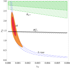
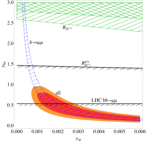
Figure 2: Left panel: $R_{D^{(*)}}$ is resolved in hatched ($2\,\sigma$) and doubly hatched ($1\,\sigma$) regions, whereas the $b\to s\mu\mu$ puzzle is resolved in dashed-hatched region at $1\,\sigma$. Region below the black line with a hatching is in $1\,\sigma$ agreement with $R_{D^{(*)}}^{\mu/e}$. No LHC constraint on $y_{b\mu}$ is considered. Right panel: Same as left panel apart from inclusion of constraint on $y_{b\mu}$ from LHC. Red and orange regions in both graphs denote $1\,\sigma$ and $2\,\sigma$ results of the fit.

5 Flavor couplings

In this section we study three scenarios differing in the number of variable Yukawas. For each scenario we report a minimum of $\chi^{2}$ function, which is a sum of terms corresponding to all observables discussed in the preceding sections. We also report $1\,\sigma$ regions for the interesting two-dimensional projections of parameter space. While performing these fits we limit all free Yukawa couplings to be smaller than $3$. Introduction of this artificial cut-off is guided by the constraints posed by the LHC searches, discussed in Sec. 6. The SM point has $\chi^{2}=71.6$ and serves as a reference value to which $\chi^{2}$ of the three fits are compared.

5.1 $S_{3}$ coupled to muons (2 parameters)

In this scenario we consider only the effect of $S_{3}$ with non-zero muonic couplings:

$$y=\begin{pmatrix}0&0&0\\ 0&y_{s\mu}&0\\ 0&y_{b\mu}&0\end{pmatrix}.$$ (42)

We set $m_{S_{3}}=1\mathrm{\,TeV}$ and for the moment ignore the direct LHC constraint on $y_{b\mu}$ spelled out in Eq. (40). In this case the best fit point has $\chi^{2}=34.7$ reached at $y_{s\mu}=5\times 10^{-4}$ and $y_{b\mu}=1.8$. The $R_{D^{(*)}}$ puzzle can be addressed by lowering $\mathcal{B}(B\to D^{(*)}\mu\nu)$ which requires large $y_{b\mu}$ coupling as seen in Eq. (10). The $1\sigma$ and $2\sigma$ regions of the fit are shown in Fig. 2. Left panel in Fig. 2 exposes tension between $R_{D^{(*)}}$ ($2.8\,\sigma$ pull) and $R_{D^{(*)}}^{\mu/e}$ ($1.8\,\sigma$ pull) which is even more exacerbated when we include the direct constraints on $y_{b\mu}$ from LHC (right panel of Fig. 2). The latter scenario with all constraints included has $\chi^{2}=42.4$ at point $(y_{s\mu},y_{b\mu})=\pm(2\times 10^{-3},0.46)$ which corresponds to the $5.0\,\sigma$ pull of the SM hypothesis. One can observe in the right panel in Fig. 2 that in this case the preferred region is drawn further away from $R_{D^{(*)}}$. The results indicate that $R_{D^{(*)}}$ cannot be explained by omitting couplings to $\tau$. Detailed results on the pulls are given in the third column of Tab. 1.

	SM	$m_{S_{3}}=1\mathrm{\,TeV}$	$m_{S_{3}}=1.0/1.5\mathrm{\,TeV}$	Eq.
		$(y_{s\mu},y_{b\mu})$	$(y_{s\mu},y_{b\mu},y_{s\tau},y_{b\tau})$
		w.o./w. Eq. (40)
$\chi^{2}$	$71.6$	$34.7/42.4$	36.8/38.0
$b\to s\ell^{+}\ell^{-}$	5.4	0.0/0.0	0.0/0.0	(14)
$R_{D^{(*)}}$	4.5	2.8/4.4	4.0/4.2	(10)
$(g-2)_{\mu}$	3.1	3.5/3.1	3.1/3.1	(30)
$R^{K}_{\tau/\mu}$	2.0	2.0/2.0	0.3/0.3	(22)
$R^{\tau/e}_{\tau}$	2.0	1.6/2.0	2.1/2.1	(25)
$\mathcal{B}(B\to\tau\nu)$	1.2	1.2/1.2	1.1/1.2	(17)
$\Delta m_{s}$	1.1	1.1/1.1	1.6/1.6	(34)
$R^{K}_{e/\mu}$	1.1	1.1/1.1	1.1/1.1	(20)
$R^{\tau/\mu}_{\tau}$	0.7	0.7/0.7	0.8/0.8	(25)
$R_{D^{(*)}}^{\mu/e}$	0.5	1.8/0.4	0.5/0.5	(16)
$R_{\nu\nu}$	0.5	0.6/0.6	0.8/0.6	(39)
$bb\to\mu\mu$	0.0	$\,-\,$/0.7	0.0/0.0	(40)
$\mathcal{B}(\tau\to\mu\gamma)$	0.0	0.0/0.0	0.4/0.3	(26)
$\mathcal{B}(B\to K\tau\mu)$	0.0	0.0/0.0	0.3/0.3	(31)

Table 1: Observables that enter the global fit with their pulls in $\sigma$ in the SM and $S_{3}$ scenarios. Third column represents the case when $m_{S_{3}}=1\mathrm{\,TeV}$ and only $y_{s\mu},y_{b\mu}$ are allowed, without/with taking into account $b\bar{b}\to\mu\mu$ constraint. Fourth column represents the fit of the $y_{s\mu}$, $y_{b\mu}$, $y_{s\tau}$, $y_{b\tau}$ scenario for $m_{S_{3}}=1.0/1.5\mathrm{\,TeV}$. The constraints with negligible pulls are not shown in this table.

5.2 $S_{3}$ coupled to muons and taus (4 parameters)

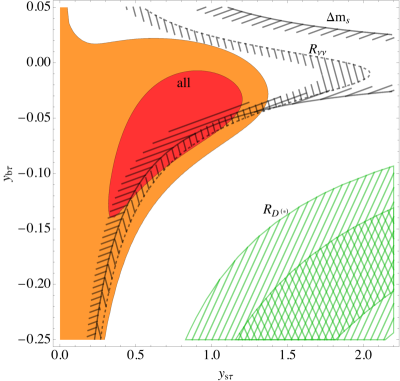
Figure 3: Fit for the $m_{S_{3}}=1\mathrm{\,TeV}$ scenario with four free couplings. $R_{D^{(*)}}$ is resolved within hatched ($2\,\sigma$) and doubly hatched ($1\,\sigma$) regions. Region to the left of the dashed line (hatched) is in $1\,\sigma$ agreement with $R_{\nu\nu}$ and $R_{\nu\nu}^{*}$. $\Delta m_{s}$ prefers (at $2\,\sigma$) a region on the hatched side of full line. Red and orange regions are $1\,\sigma$ and $2\,\sigma$ results of the fit.

Since the purely muonic couplings are in conflict with $R_{D^{(*)}}$ we allow in addition for tauonic couplings of $S_{3}$:

$$y=\begin{pmatrix}0&0&0\\ 0&y_{s\mu}&y_{s\tau}\\ 0&y_{b\mu}&y_{b\tau}\end{pmatrix}.$$ (43)

In this case both couplings with the muons tend to be small, below $0.1$, and are relevant only in $b\to s\mu\mu$, whereas the couplings to $\tau$ are $\sim 1$ in order to enhance $R_{D^{(*)}}$. For $m_{S_{3}}=1\mathrm{\,TeV}$ we find that the minimal $\chi^{2}$ of this scenario with 4 degrees of freedom is $36.8$ reached at $(y_{s\mu},y_{b\mu},y_{s\tau},y_{b\tau})=(0.047,0.020,0.87,-0.048)$ which makes the SM point excluded at $5.0\,\sigma$ (pull). In Fig. 3 the fit in the tauonic couplings’ plane shows how the optimal region is still far from the central value of $R_{D^{(*)}}$, mostly due to $R_{\nu\nu}$ and $\Delta m_{s}$, which do not allow for large products of $y_{b\tau}y_{s\tau}$. Pulls of individual observables for $m_{S_{3}}=1.0/1.5\mathrm{\,TeV}$ are presented in the fourth column of Table 1.

5.3 $S_{3}$ and $\tilde{R}_{2}$ (6 parameters)

In order to relax the tension in the $y_{s\tau}$–$y_{b\tau}$ plane between large effect in $R_{D^{(*)}}$ and well constrained $R_{\nu\nu}^{(*)}$ and $\Delta m_{s}$, we could invoke a light $\tilde{R}_{2}$ with couplings to $\tau$. We consider a case $m_{S_{3}}=m_{\tilde{R}_{2}}=1\mathrm{\,TeV}$ with six free Yukawa couplings ($y_{ij}$ from the previous subsection and $(\tilde{y}_{s\tau},\tilde{y}_{b\tau})$ pair) to find $\chi^{2}=33.4$ at $(y_{s\mu},y_{b\mu},y_{s\tau},y_{b\tau})=(0.051,0.019,0.86,-0.069)$, $(\tilde{y}_{s\tau},\tilde{y}_{b\tau})=(3,0.0026)$ that represents a $4.9\,\sigma$ pull of the SM. Most importantly, the tension in $R_{D^{(*)}}$ is only marginally improved and stands at $3.7\,\sigma$. The presence of $\tilde{R}_{2}$ allows for partial cancellation in $\Delta m_{s}$ between large tauonic couplings of $S_{3}$ and $\tilde{R}_{2}$, which is not the case in both $R_{\nu\nu}$ and $R_{\nu\nu}^{*}$, where cancellation in one observable necessary spoils the other (cf. (39)). We thus conclude that light $\tilde{R}_{2}$ with relatively large couplings to the SM fermions cannot improve substantially the agreement with data. We accordingly assume that the couplings of $\tilde{R}_{2}$, i.e., $\tilde{y}_{ij}$ of Eq. (5), are small enough as not to affect flavor observables. With light $\tilde{R}_{2}$ and its Yukawa couplings sufficiently small to avoid flavor constraints we can still aid gauge coupling unification and generate viable neutrino masses in the underlying GUT model as we show in Sec. 7.

6 Collider constrains

In what follows we confront our model, comprising two light LQs, with collider constraints while taking into account the particularities of the flavor structure derived in the previous section. We demonstrate the viability of the proposed model and present bounds from third generation LQ pair production as well as high-mass $\tau\tau$ production searches at the 13 TeV LHC for current and projected luminosities. We show that a large portion of the relevant parameter space can be covered by the HL-LHC.

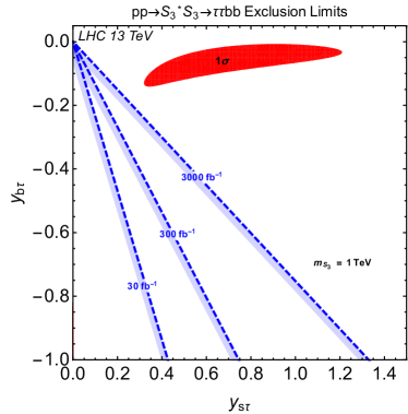
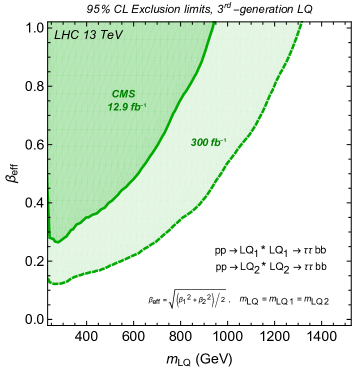
Figure 4: (Left Panel) 95% C.L. exclusion limits from LQ pair production (dotted blue lines) at different projected LHC luminosities for a 1 TeV $S_{3}$ LQ. The red region corresponds to the 1 $\sigma$ low energy fit. (Right panel) Reinterpretation of the CMS Collaboration exclusion limits for two generic degenerate LQs decaying into $\tau\tau bb$ final state in the $\beta_{\text{eff}}$–$m_{\mathrm{LQ}}$ plane.

6.1 LQ pair production

The current best mass limit for LQs that decay to the third-generation leptons has been recently reported by the CMS Collaboration while searching for a pair of QCD produced LQs decaying into the $\tau^{+}\tau^{-}b\bar{b}$ channel Sirunyan:2017yrk . This search excludes an LQ with mass bellow $850$ GeV (550 GeV) for a branching ratio (BR) of $\beta=1$ ($\beta=0.5$). This search can set limits on the parameter space of our model via $pp\!\to\!S_{3}^{4/{3}^{*}}S_{3}^{4/3}(\tilde{R}_{2}^{2/{3}^{*}}\tilde{R}_{2}^{2/3})\to\tau^{+}\tau^{-}b\bar{b}$ processes.

We focus on the scenario presented in Sec. 5.2 when $S_{3}$ is at the TeV scale and $\tilde{R}_{2}$ is assumed not to feed significantly in the $\tau^{+}\tau^{-}b\bar{b}$ signal. In this case the CMS bound can be applied directly to the $S_{3}^{4/{3}}$ state, at a benchmark mass of $m_{S_{3}}=1$ TeV, decaying into a $\tau b$ pair with a BR given by

$$\beta\approx\frac{|y_{b\tau}|^{2}}{|y_{b\tau}|^{2}+|y_{s\tau}|^{2}}\,.$$ (44)

Here we neglect the small widths of $S_{3}^{4/3}$ into both muonic channels. Results are given in Fig. 4 (left panel), where the dashed blue contours represent the 95% C.L. exclusion limits for different LHC luminosities and the red region represents the $1\,\sigma$ region for the low-energy fit derived in Sec. 5.2. It is worth mentioning that we did not include other contributions which could potentially tighten these bounds, for example, contributions from $pp\to S_{3}^{4/{3}^{*}}S_{3}^{4/3}\to\tau^{+}\tau^{-}bs$. The search starts losing sensitivity for $m_{S_{3}}$ above 1 TeV, while for masses larger than $1.2$ TeV the search does not produce any useful limits. In conclusion, a third generation LQ pair production search at the LHC is not a sensitive probe for this particular flavor structure of our LQ model.

We now turn to the scenario where two generic third generation LQs (like e.g. $S_{3}$ and $\tilde{R}_{2}$) are at the TeV scale and both contribute to LQ pair production. A naive reinterpretation of the CMS limits Sirunyan:2017yrk can be performed when (i) both LQ components are degenerate in mass, (ii) interference terms between the final state $\tau b$ pairs at the amplitude level are negligible and, (iii) the LQ decay widths are small enough in order to guarantee the narrow width approximation (NWA) assumed in the experimental search. This scenario would thus correspond to the particular case we investigated in Sec. 5.3.

As shown in Appendix A, the CMS bound for one LQ can be directly mapped into a bound for two degenerate LQs we denote with $\mathrm{LQ}_{1}$ and $\mathrm{LQ}_{2}$, for simplicity, when the associated BRs are $\beta_{1}$ and $\beta_{2}$, respectively. (See Fig. 2 (right panel) of Ref. Sirunyan:2017yrk for the experimental limit.) The inferred limits, which apply in general to two third-generation LQs with non-interfering final states, are presented in Fig. 4 (right panel) for an integrated luminosity of 12.9 fb^-1 (solid green contour). For example, we find that both LQs with equal masses bellow 930 GeV (600 GeV) are excluded at 95% C.L. if $\beta_{\text{eff}}=1$ ($\beta_{\text{eff}}=0.5$), where $\beta_{\text{eff}}=\sqrt{(\beta_{1}^{2}+\beta_{2}^{2})/2}$. We also include LHC projections for an integrated luminosity of 300 fb^-1 (dashed green contour) by rescaling the CMS Collaboration limits with the square root of the luminosity ratio. At this projected luminosity the LQ pair production search is not sensitive for masses above $1.3$ TeV. These results, again, can be used for our LQ model for degenerate $S_{3}$ and $\tilde{R}_{2}$ LQs at the TeV scale. Unfortunately, the LHC bounds on the couplings extracted from LQ pair production search are not strong enough to probe this scenario either.

6.2 High-mass $\tau\tau$ production

In this section we study the implication of light $S_{3}$ and $\tilde{R}_{2}$ leptoquarks for high-$p_{T}$ $\tau\tau$ production at the LHC. It was shown in Refs. Faroughy:2016osc ; Greljo:2015mma that $\tau\tau$ resonance searches at the LHC produce stringent constrains on a large class of models explaining the $R_{D^{(*)}}$ anomaly. In what follows we give predictions for the deviation from the SM in the invariant mass tails of $pp\to\tau^{+}\tau^{-}$ and derive bounds at different luminosities for the parameter space of the present LQ model from the 13 TeV ATLAS Collaboration resonance search at 3.2 fb^-1 Aaboud:2016cre .

Both LQs contribute to $pp\to\tau^{+}\tau^{-}$ production exclusively through Yukawa interactions by exchanging $S_{3}^{4/3}$, $S_{3}^{1/3}$, and $\tilde{R}_{2}^{2/3}$ components in the $t$-channel from partonic $q\bar{q}$ annihilation. The relevant Feynman diagrams are depicted in Fig. 5. Potentially large contributions may come from the processes with incoming strange quarks $s\bar{s}\to\tau^{+}\tau^{-}$ and $s\bar{b}\,(b\bar{s})\to\tau^{+}\tau^{-}$, followed by sub-leading contributions from bottom, charm and up quark initiated processes $b\bar{b}\,(c\bar{c})\,(u\bar{u})\to\tau^{+}\tau^{-}$. The flavor structure in Eq. (4) also allows for $S_{3}^{1/3}$ to couple to $u$ and $\tau$ via the CKM mixing. Nevertheless, this coupling is proportional to $|V_{us}|\,y_{s\tau}$, meaning that $\tau\tau$ production from incoming up quarks is Cabibbo suppressed leading to negligible cross-sections of order $|V_{us}|^{2}$ and $|V_{us}|^{4}$ for the processes $c\bar{u}\to\tau^{+}\tau^{-}$ and $u\bar{u}\to\tau^{+}\tau^{-}$, respectively. The Cabibbo suppressed vertices are shown in red in Feynman diagrams of Fig. 5. On the other hand, at high-$x$ the large proton PDF of the valence up quark in the process $u\bar{c}\to\tau^{+}\tau^{-}$ can marginally compensate for the $|V_{us}|$ suppression in the amplitude giving a contribution comparable to $c\bar{c}\to\tau^{+}\tau^{-}$ in the total cross-section.

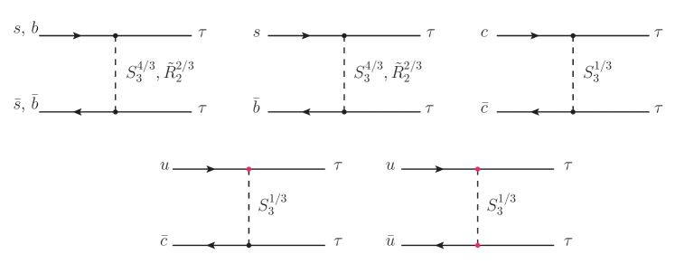
Figure 5: Leading order Feynman diagrams for the $t$-channel $S_{3}$ and $\tilde{R}_{2}$ exchanges in $pp\to\tau^{+}\tau^{-}$ process. The red vertex indicates the presence of the $|V_{us}|$ Cabibbo suppression in the coupling.

We now focus on the total cross-section $\sigma^{\text{fid}}_{\text{TOT}}$ of $pp\to\tau^{+}\tau^{-}$ far from the $Z$-pole in the high-mass tails of the $\tau\tau$ invariant mass distribution. We will, for definiteness, study the scenario where only $S_{3}$ contributes to $\tau\tau$ production. The couplings of $\tilde{R}_{2}$ are assumed to be small and can thus be safely neglected for this collider study. This is in accordance with the outcome of the numerical study presented in Sec. 5.2.

At leading-order (LO), $\tau\tau$ production will receive contributions from the $t$-channel exchange of $S_{3}$, from the $s$-channel SM Drell-Yan $pp\to Z/\gamma^{*}\to\tau\tau$ production, and from interference effects between these processes. The high-mass kinematic region is defined by the following fiducial cuts on the final states: $p_{T}>100$ GeV (50 GeV) for the leading (sub-leading) $\tau$ and a high invariant mass cut for the $\tau\tau$ pair of $m_{\tau\tau}>600$ GeV. We define the signal strength $\mu_{pp\to\tau\tau}$ as the ratio of $\sigma^{\text{fid}}_{\text{TOT}}$ with the the SM Drell-Yan fiducial cross-section $\sigma^{\text{fid}}_{\text{SM}}$:

$$\mu_{pp\to\tau\tau}\ \equiv\ \sigma^{\text{fid}}_{\text{TOT}}\,/\,\sigma^{\text{fid}}_{\text{SM}}\ =\ 1\ +\ \sigma^{\text{fid}}_{\text{LQ}}\,/\,\sigma^{\text{fid}}_{\text{SM}}\,.$$ (45)

Here the fiducial cross-section $\sigma^{\text{fid}}_{\text{LQ}}$ includes all NP contributions from both the LQ squared and LQ-SM interference amplitudes, i.e., $\sigma^{\text{fid}}_{\text{LQ}}=2\,\text{Re}(\mathcal{A}_{\text{SM}}^{*}\mathcal{A}_{\text{LQ}})\,+\,|\mathcal{A}_{\text{LQ}}|^{2}$. The ratio $\sigma^{\text{fid}}_{\text{LQ}}\,/\,\sigma^{\text{fid}}_{\text{SM}}$ quantifies the NP deviation of the total fiducial cross-section from the expected SM prediction. The LQ Yukawa couplings enter in $\sigma^{\text{fid}}_{\text{LQ}}$ as

$$\sigma^{\text{fid}}_{\text{LQ}}(y_{s\tau},y_{b\tau})\ =\ \sigma_{s\bar{s}}\,(y_{s\tau})\ +\ \sigma_{s\bar{b}}\,(y_{s\tau},y_{b\tau})\ +\ \sigma_{b\bar{b}}\,(y_{b\tau})\ +\ \sigma_{c\bar{c},u\bar{u},u\bar{c}}\,(y_{s\tau}),$$ (46)

In order to conform with the analysis in Sec. 5 we assume all Yukawa couplings to be real. Here $\sigma_{s\bar{s}}$, $\sigma_{s\bar{b}}$, $\sigma_{b\bar{b}}$ and $\sigma_{c\bar{c},u\bar{u},u\bar{c}}$ correspond to the fiducial cross-sections of the processes $s\bar{s}\to\tau^{+}\tau^{-}$, $s\bar{b}\,(\bar{s}b)\to\tau^{+}\tau^{-}$, $b\bar{b}\to\tau^{+}\tau^{-}$ and $c\bar{c}\,(u\bar{u})\,(u\bar{c})\to\tau^{+}\tau^{-}$ respectively. These can be expressed as generic quartic polynomials in the couplings:

$$\sigma_{s\bar{s}}\,(y_{s\tau}) = y_{s\tau}^{4}\,A_{1}\ +\ y_{s\tau}^{2}\,B_{1}\,,$$ (47)

$$\sigma_{s\bar{b}}\,(y_{s\tau},y_{b\tau}) = y_{s\tau}^{2}y_{b\tau}^{2}\,A_{2}\,,$$ (48)

$$\sigma_{b\bar{b}}\,(y_{b\tau}) = y_{b\tau}^{4}\,A_{3}\ +\ y_{b\tau}^{2}\,B_{3}\,,$$ (49)

$$\sigma_{c\bar{c},u\bar{u},u\bar{c}}\,(y_{s\tau}) = y_{s\tau}^{4}\,A_{4}\ -\ y_{s\tau}^{2}\,B_{4}\,.$$ (50)

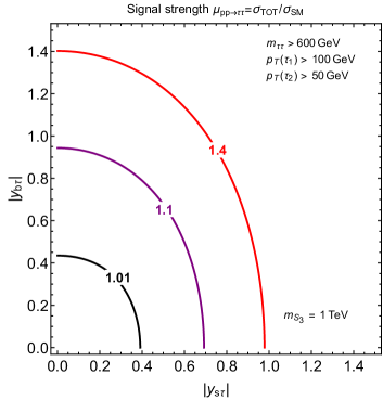
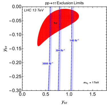
Figure 6: (Left panel) Contours of constant signal strength $\mu_{pp\to\tau\tau}$ for different deviations from the SM prediction at $m_{S_{3}}=1$ TeV. (Right panel) 95% C.L. limits for LHC luminosities of 100, 300, and, 3000 fb^-1 (dotted blue contours) from recasting high-mass $\tau\tau$ searches by ATLAS Aaboud:2016cre for $m_{S_{3}}=1$ TeV. The red region corresponds to the 1 $\sigma$ low-energy fit.

The polynomial coefficients $A_{i}$ and $B_{i}$ are functions of the mass $m_{S_{3}}$ describing the LQ squared amplitudes and LQ-SM interference amplitudes, respectively. In Eqs. (47)–(50) we define all polynomial coefficients to be positive and include the explicit signs of the LQ-SM interference coefficients $B_{i}$, indicating the presence of either destructive or constructive interference amplitudes. The origin of the sign of these interference terms can be traced back to the SM amplitude proportional to the $T_{3}-\sin^{2}\theta_{W}\,Q$ coupling of the $Z$ boson with the incoming quarks along with the sign of the LQ Yukawa interactions of $S_{3}^{4/3\,(1/3)}$. The interference arising between the $Z$ boson and the $S_{3}^{4/3\,(1/3)}$ components is driven by the weak isospin of the quark doublets, i.e., positive (negative) for up(down)-type quarks. This translates into a constructive interference for down-type quarks in $d\bar{d},\,s\bar{s}\,,b\bar{b}\to\tau\tau$ processes and destructive interference for up-type quarks in $c\bar{c}\,,u\bar{u}\to\tau\tau$ processes. As a consequence, this relative sign that appears between the LQ-SM interferences in different $\tau\tau$ production channels leads to a partial cancellation in the cross-section $\sigma^{\text{fid}}_{\text{LQ}}$. For more details see Appendix B.

For the calculations below we choose a benchmark mass value of 1 TeV. In order to extract the values of the polynomial coefficients $A_{i}$ and $B_{i}$ we generate in FeynRules Alloul:2013bka the UFO model file for the Lagrangian for $S_{3}$ and simulate in MadGraph5 Alwall:2014hca 13 TeV event samples of $pp\to\tau^{+}\tau^{-}$ subject to the high-mass fiducial cuts discussed above for different values of the couplings. The specific values of the coefficients can be found in Appendix B. In Fig. 6 (left panel) we show results for different contours of constant signal strength $\mu_{pp\to\tau\tau}$ in the $y_{s\tau}$–$y_{b\tau}$ plane for the 1 TeV mass scenario. This shows that our LQ model equipped with the proposed flavor structure with $y_{s\tau,b\tau}$ couplings of $\mathcal{O}(1)$, predicts at the LHC an enhancement of $\mathcal{O}(10\%)$ in the $\tau\tau$ tails when compared to the SM.

In the remaining part of this section we confront our model with existing LHC data and extract $95\%$ C.L. limits for the model parameters at different integrated luminosities. For this we recast a heavy $Z^{\prime}$ search by the ATLAS Collaboration with $3.2$ fb^-1 of data in the fully hadronic $\tau_{\text{had}}\tau_{\text{had}}$ channel Aaboud:2016cre . For the recast we generate at LO in MadGraph5 a set of the LQ $\tau_{\text{had}}\tau_{\text{had}}$ signal samples followed by parton showering and hadronization in Pythia8 Sjostrand:2014zea . We have included interference effects between the LQ signals and the SM Drell-Yan background process. Detector effects are simulated in Delphes3 deFavereau:2013fsa with settings tuned according to the experimental environment of the $\tau_{\text{had}}\tau_{\text{had}}$ inclusive category as described in Ref. Aaboud:2016cre . For this category, events are selected if the reconstructed objects satisfies the following requirements:

• $p_{T}>110$ GeV (55 GeV) for the leading (sub-leading) $\tau_{\text{had}}$.

• Events with isolated electrons (muons) are vetoed if $p_{T}>10$ GeV ($p_{T}>15$ GeV).

• Opposite sign $\tau_{\text{had}}\tau_{\text{had}}$ with back-to-back topology in the transverse plane, $\Delta\phi(\tau_{\text{had}}\tau_{\text{had}})>2.7$.

• Total transverse mass cut of $m_{T}^{\text{tot}}>350$ GeV.

Here $m_{T}^{\text{tot}}$ is the dynamical variable used to reconstruct the invariant mass of the visible part of $\tau_{\text{had}}\tau_{\text{had}}$ defined as $({m_{T}^{\text{tot}}})^{2}\equiv m_{T}^{2}(\tau_{1},\tau_{2})+m_{T}^{2}(\tau_{1},E^{\text{miss}}_{T})+m_{T}^{2}(\tau_{2},E^{\text{miss}}_{T})$ where $E^{\text{miss}}_{T}$ is the total missing energy in the event and $m_{T}^{2}(A,B)=p_{T}(A)p_{T}(B)(1-\cos\Delta\phi(A,B))$ is the squared transverse mass of objects $A$ and $B$. In order to extract limits from the tails of the $m_{T}^{\text{tot}}$ distributions we use the statistical analysis presented in Ref. Faroughy:2016osc . For $m_{\mathrm{LQ}}>1$ TeV the most sensitive bin corresponds to the last one ($m_{T}^{\text{tot}}>684$ GeV) where a point in parameter space is excluded at 95% C.L. if the number of events in that bin exceeds 11, 36 and 113 at integrated luminosities of 30, 300, 3000 fb^-1 respectively. Here we have applied a naive scaling of the limits for the 3.2 fb^-1 search to arbitrary luminosities with $\sqrt{\mathcal{L}_{\text{int}}/3.2\,\small{\text{fb}^{-1}}}$. The results are given in Fig. 6 (Right panel) for the benchmark mass of $m_{\mathrm{LQ}}=1$ TeV. There the regions to the right of the dotted blue boundaries are excluded at 95% C.L. for future LHC luminosities of 30 fb^-1, 300 fb^-1 and 3000 fb^-1. In the plot we have also included the $1\,\sigma$ region in solid red obtained from the low-energy fit to all flavor experiments performed in Sec. 5.2. Notice that these bounds are conservative given that we have not included NLO QCD corrections and have not taken into account other processes such as non-resonant $qg\to\tau\tau q$ that can produce sizeable contributions to the inclusive $\tau_{\text{had}}\tau_{\text{had}}$ category . From these results we conclude that the High-Luminosity LHC can probe a large portion of the parameter space for the Yukawa coupling ansatz of Sec. 5.2.

7 GUT completion

The preceding sections were devoted to the study of the impact of light scalar fields $S_{3}$ and $\tilde{R}_{2}$ with potentially sizeable couplings to the quark-lepton pairs on the flavor physics processes and LHC observables. Here we want to demonstrate that these fields and associated couplings can originate from a consistent grand unified theory (GUT) model.

To insure that the LHC accessible leptoquarks $S_{3}$ and $\tilde{R}_{2}$ are not in conflict with stringent limits on matter stability it is necessary that both $S_{3}$ and $\tilde{R}_{2}$ do not couple to the quark-quark pairs either directly or through the mixing with other scalars in a specific model of unification. It turns out that one can meet this requirement in an $SU(5)$ model that comprises $5$-, $15$-, $24$-, and $45$-dimensional scalar representations Dorsner:2017wwn . The decomposition of the scalar sector of that model is $\bm{5}=(\Psi_{D},\Psi_{T})=(\bm{1},\bm{2},1/2)\oplus(\bm{3},\bm{1},-1/3),$ $\bm{15}=(\Phi_{a},\Phi_{b},\Phi_{c})=(\bm{1},\bm{3},1)\oplus(\bm{3},\bm{2},1/6)\oplus(\bm{6},\bm{1},-2/3)$, $\bm{24}=(\Sigma_{8},\Sigma_{3},\Sigma_{(3,2)},\Sigma_{(\overline{3},2)},\Sigma_{24})=(\bm{8},\bm{1},0)\oplus(\bm{1},\bm{3},0)\oplus(\bm{3},\bm{2},-5/6)\oplus(\overline{\bm{3}},\bm{2},5/6)\oplus(\bm{1},\bm{1},0)$, and $\bm{45}=(\Delta_{1},\Delta_{2},\Delta_{3},\Delta_{4},\Delta_{5},\Delta_{6},\Delta_{7})=(\bm{8},\bm{2},1/2)\oplus(\overline{\bm{6}},\bm{1},-1/3)\oplus(\bm{3},\bm{3},-1/3)\oplus(\overline{\bm{3}},\bm{2},-7/6)\oplus(\bm{3},\bm{1},-1/3)\oplus(\overline{\bm{3}},\bm{1},4/3)\oplus(\bm{1},\bm{2},1/2)$, where $\Phi_{b}$ and $\Delta_{3}$ are identified with $\tilde{R}_{2}$ and $S^{*}_{3}$, respectively. The fermions of the SM, on the other hand, are embedded within the tenplets and fiveplets in the usual manner Georgi:1974sy .

We first show that this GUT scenario is compatible with the viable gauge coupling unification. To this end, we take all scalar fields in the model that mediate proton decay at tree-level to reside at or above $10^{12}$ GeV. These fields are $\Psi_{T}$, $\Delta_{5}$, and $\Delta_{6}$ Dorsner:2017wwn . We furthermore set the masses of both $S_{3}$ and $\tilde{R}_{2}$ at $1$ TeV and constrain all remaining scalar fields to be at or above one scale we simply denote $m$ that is to be determined through the requirement that the gauge coupling unification takes place at the one-loop level. Note that $\Sigma_{24}$ does not affect unification. Also, $\Sigma_{(3,2)}$ and $\Sigma_{(\overline{3},2)}$ are not physical fields since they provide necessary degrees of freedom for the baryon and lepton number violating gauge bosons $X$ and $Y$ of the $SU(5)$ origin to become massive fields.

The gauge couplings meet at the unification scale $m_{\mathrm{GUT}}$ when the following equation is satisfied Giveon:1991zm

$$\frac{B_{23}}{B_{12}}=\frac{5}{8}\frac{\sin^{2}\theta_{W}-\alpha/\alpha_{S}}{3/8-\sin^{2}\theta_{W}}=0.721\pm 0.004,$$ (51)

where the right-hand side is evaluated using $\alpha_{S}(m_{Z})=0.1193\pm 0.0016$, $\alpha^{-1}(m_{Z})=127.906\pm 0.019$, and $\sin^{2}\theta_{W}=0.23126\pm 0.00005$ Agashe:2014kda . The left-hand side depends on the particle content and the mass spectrum of the model. Namely, coefficients $B_{ij}$ are $B_{ij}=\sum_{J}(b^{J}_{i}-b^{J}_{j})r_{J}$, where $b^{J}_{i}$ are the well-known $\beta$-function coefficients of particle $J$ with mass $m_{J}$ and $r_{J}=(\ln m_{\mathrm{GUT}}/m_{J})/(\ln m_{\mathrm{GUT}}/m_{Z})$. The sum goes through all particles beside the SM ones that reside between $Z$ boson mass $m_{Z}$ and $m_{\mathrm{GUT}}$. The convention is such that $b^{J}_{1}$, $b^{J}_{2}$, and $b^{J}_{3}$ are associated with $U(1)$, $SU(2)$, and $SU(3)$ of the SM, respectively. We identify $m_{\mathrm{GUT}}$ not only with the gauge coupling unification scale but with the masses of the proton decay mediating gauge boson fields $X$ and $Y$.

If and when unification takes place for a given $m$ we evaluate $m_{\mathrm{GUT}}$ using equation Giveon:1991zm

$$\ln\frac{m_{\mathrm{GUT}}}{m_{Z}}=\frac{16\pi}{5\alpha}\frac{3/8-\sin^{2}\theta_{W}}{B_{12}}=\frac{184.8\pm 0.1}{B_{12}}$$ (52)

to check that $m_{\mathrm{GUT}}\geq 5\times 10^{15}$ GeV in order to satisfy stringent bounds on the $X$ and $Y$ gauge boson mediated proton decay. To actually set a lower bound on $m$ we fix $m_{\mathrm{GUT}}=5\times 10^{15}$ GeV in our analysis and maximise $m$. We find that $m=3.1\times 10^{10}$ GeV when the masses of both $\tilde{R}_{2}$ and $S_{3}$ are at $1$ TeV. The masses of all other scalar particles in the model are $m_{\Psi_{D}}=10^{2}$ GeV, $m_{\Psi_{T}}=10^{12}$ GeV, $m_{\Phi_{a}}=m_{\mathrm{GUT}}$, $m_{\Phi_{c}}=m$, $m_{\Sigma_{8}}=m$ , $m_{\Sigma_{3}}=m_{\mathrm{GUT}}$, $m_{\Delta_{1}}=m$, $m_{\Delta_{2}}=m$, $m_{\Delta_{4}}=1.2\times 10^{12}$ GeV, $m_{\Delta_{5}}=10^{12}$ GeV, and $m_{\Delta_{6}}=10^{12}$ GeV, $m_{\Delta_{7}}=m_{\mathrm{GUT}}$. Note that the SM Higgs is in principle a mixture of $\Psi_{T}$ and $\Delta_{7}$. We accordingly take one state to be light and treat the mass of the other as a free parameter that is between $m$ and $m_{\mathrm{GUT}}$.

The fact that viable unification can take place when $S_{3}$ and $\tilde{R}_{2}$ are both light does not come as a surprise. Note that the SM field content yields $B^{\textrm{SM}}_{23}/B^{\textrm{SM}}_{12}=0.53$ instead of the experimentally required value given in Eq. (51). The nice feature of the set-up with light $S_{3}$ and $\tilde{R}_{2}$ is that both fields have positive $b^{J}_{23}$ and negative $b^{J}_{12}$ coefficients. This not only helps in bringing the left-hand side of Eq. (51) in agreement with the required experimental value but simultaneously raises the GUT scale $m_{\mathrm{GUT}}$ through Eq. (52). The relevant coefficients are $b^{S_{3}}_{23}=9/6$, $b^{S_{3}}_{12}=-27/15$, $b^{\tilde{R}_{2}}_{23}=1/6$, and $b^{\tilde{R}_{2}}_{12}=-7/15$. Again, our findings demonstrate that the gauge coupling unification is possible for light $S_{3}$ and $\tilde{R}_{2}$ in this particular model.

We next demonstrate that the explicit forms of the Yukawa couplings of $S_{3}$ and $\tilde{R}_{2}$ that are used in Sec. 5 to produce numerical fits can originate from the appropriate $SU(5)$ operators. It is also argued that the model can accommodate realistic masses of the SM fermions.

The $S_{3}\in\overline{\bm{45}}$ lepton-quark couplings originate from the $SU(5)$ contraction $y^{45}_{ij}\bm{10}_{i}\overline{\bm{5}}_{j}\overline{\bm{45}}$, where $\bm{10}_{i}$ are the usual fermionic tenplets, $i(=1,2,3)$ is the generation index, and $y^{45}$ is a $3\times 3$ matrix in flavor space. We can thus identify $y$ of Eq. (3) with $y^{45}/\sqrt{2}$, where $y^{45}$ is related to the difference in masses between charged fermions and down-type quarks Dorsner:2017wwn . This follows from the fact that there are actually two operators that contribute towards the charged fermion and down-type quark masses in this $SU(5)$ model Georgi:1979df . One is $y^{45}_{ij}\bm{10}_{i}\overline{\bm{5}}_{j}\overline{\bm{45}}$ and the other is $y^{5}_{ij}\bm{10}_{i}\overline{\bm{5}}_{j}\overline{\bm{5}}$, where $y^{5}$ is an arbitrary complex matrix. Clearly, $y^{45}=\sqrt{2}y$ and $y^{5}$ together contain enough parameters to easily address observed mismatch between the charged fermion and down-type quark masses. For completeness we specify that the up-type quark masses originate from a single contraction $x_{ij}\bm{10}_{i}\bm{10}_{j}\bm{5}$, where $x_{ij}$ is a symmetric complex $3\times 3$ matrix.

The $\tilde{R}_{2}\in\bm{15}$ lepton-quark couplings are symmetric in flavor space since they originate from $y^{15}_{ij}\overline{\bm{5}}_{i}\overline{\bm{5}}_{j}\bm{15}$, where $\overline{\bm{5}}_{i}$ are the usual fermionic fiveplets. We identify $\tilde{y}_{ij}$ of Eq. (5) with $-(D_{R}y^{15})_{ij}/\sqrt{2}$ in the physical basis for the down-type quarks and charged leptons, where $D_{R}$ represents unitary transformation of the right-chiral down-type quarks. If we take that $y^{15}_{33}\neq 0$ we obtain the form of $\tilde{y}$ that is used in the fit of Sec. 5 when we consider joint effect of $S_{3}$ and $\tilde{R}_{2}$ on flavor observables.

It is worth mentioning that it is possible to address neutrino masses within this model. Namely, if one turns on a vacuum expectation value of the electrically neutral field $\Phi_{a}\in\bm{15}$ one can generate neutrino masses of Majorana nature via type II see-saw mechanism Lazarides:1980nt ; Mohapatra:1980yp through the same operator that yields the $\tilde{R}_{2}$ lepton-quark couplings, i.e., $y^{15}_{ij}\overline{\bm{5}}_{i}\overline{\bm{5}}_{j}\bm{15}$. In this particular instance the entries in $y^{15}$ would need to be responsible for the observed mass-squared differences and mixing angles in the neutrino sector. That requirement would not be compatible with a simple ansatz for the structure of $\tilde{y}$ given in Eq. (6). Again, viable neutrino masses would only be possible if we depart from that ansatz and assume that the $\tilde{y}_{ij}$ entries are sufficiently small to avoid flavor constraints for light $\tilde{R}_{2}$. This is in agreement with the findings we presented in Sec. 5.3. Note that the neutrino Majorana masses could also receive partial contribution through the one-loop processes, where the particles in the loop are down-quarks and a mixture of $S_{3}$ and $\tilde{R}_{2}$ Chua:1999si ; Mahanta:1999xd ; Dorsner:2017wwn .

The preceding discussion demonstrates that the $SU(5)$ GUT model comprising $5$-, $15$-, $24$-, and $45$-dimensional scalar representations, with the canonical embedding of the SM fermions, can accommodate light $S_{3}$ and $\tilde{R}_{2}$ and describe observed fermion masses of the SM without any conflict with relevant experimental constraints.

8 Conclusion

Our aim, in the present work, is to accommodate the observed lepton non-universality in charged current processes, signalled by $R_{D^{(*)}}$, as well as lepton non-universality and the global tension in the $b\to s\mu^{+}\mu^{-}$ sector through the introduction of light scalar LQ $S_{3}$. This LQ emerges naturally in the context of a specific $SU(5)$ GUT model and has to be accompanied by another light scalar LQ $\tilde{R}_{2}$ which improves gauge coupling unification and aids neutrino mass generation.

The first state, $S_{3}$, couples left-handed $s$ and $b$ to left-handed $\mu$ and $\tau$ and is capable of accommodating $b\to s\ell^{+}\ell^{-}$ sector. Because of its weak triplet nature it also couples to up-type quarks and neutrinos which are precisely the additional couplings needed to address $R_{D^{(*)}}$. Large couplings needed for $R_{D^{(*)}}$ cause the weak triplet $S_{3}$ to inevitably contribute to other well constrained flavor observables that agree with the SM predictions. We have analyzed those in detail and demonstrated that the most pressing ones, $R_{\nu\nu}^{(*)}=\mathcal{B}(B\to K^{(*)}\bar{\nu}\nu)/\mathcal{B}(B\to K^{(*)}\bar{\nu}\nu)_{\mathrm{SM}}$ and $\Delta m_{s}$, allow only for minor improvement of $R_{D^{(*)}}$ puzzle. We furthermore show that the second state, $\tilde{R}_{2}$, cannot significantly improve the agreement with data.

Based on the numerical values of the LQ Yukawa couplings as obtained in the flavor fit we recast two LQ collider searches: (i) search for pair produced LQs decaying to $b\tau b\tau$, (ii) search for high-mass $\tau\tau$ final state which is sensitive to the $t$-channel LQ exchange. From the recast of the search for the LQ pair production we find that the proposed scenario with $m_{S_{3}}=1\mathrm{\,TeV}$ cannot be significantly probed in a large portion of the parameter space even with $300\mathrm{\,fb}^{-1}$ of integrated luminosity at the Large Hadron Collider. Complementary searches for $\tau\tau$ final states produced via a single LQ exchange, on the other hand, are not as hampered by large LQ masses and are already excluding corners of the parameter space with largest individual Yukawa couplings. Moreover, since the flavor fit requires increasing Yukawa couplings for larger LQ masses the sensitivity of high-mass $\tau\tau$ final state search does not degrade at higher masses as compared to the pair production mechanism. This method can probe almost entire parameter space of the model at $3000\mathrm{\,fb}^{-1}$ of integrated luminosity.

A natural ultraviolet completion for the two LQ states is an $SU(5)$ GUT. We demonstrate that a particular setting with $5$-, $15$-, $24$-, and $45$-dimensional scalar representations is consistent with unification of the gauge couplings, where light $S_{3}$ and $\tilde{R}_{2}$ leptoquarks reside in $45$- and $15$-dimensional representations, respectively. Furthermore, baryon number violation is sufficiently suppressed by lack of diquark couplings of $S_{3}$ and high enough scale of the rest of the GUT spectrum. The model also accommodates the masses of all fermions of the SM.

Appendix A LQ pair production recast

In this appendix we give a reinterpretation of the results by the CMS Collaboration Sirunyan:2017yrk for the case of two LQs, denoted LQ₁ and LQ₂. When addressing the LQ pair production from QCD interactions, a model with two LQs of degenerate mass $m_{\mathrm{LQ}}\equiv m_{\mathrm{LQ}_{1}}=m_{\mathrm{LQ}_{2}}$ with BRs $\beta_{1}$ and $\beta_{2}$ for LQ${}_{1}\to\tau b$ and LQ${}_{2}\to\tau b$, respectively, can be consistently mapped to a model with only one LQ, denoted here as $\mathrm{LQ}$, with an effective mass $m_{\text{eff}}$ and an effective BR $\beta_{\text{eff}}$ for LQ $\to\tau b$. In this case, assuming the NWA, the total cross-section for $pp\to\mathrm{LQ}^{*}\mathrm{LQ}\to\tau^{+}\tau^{-}b\bar{b}$ is factorized into production and decay modes as

$$\sigma_{pp\to\tau\tau bb}=\beta_{\text{eff}}^{2}\times\sigma_{\text{pair}}(m_{\text{eff}}),$$ (53)

where $\sigma_{\text{pair}}$ is the $pp\to\mathrm{LQ}^{*}\mathrm{LQ}$ pair production cross-section that depends exclusively on the LQ mass when only QCD interactions are taken into account. For the numerical calculations we use the approximate expression from Ref. Mandal:2015lca for the cross-section at NLO

$$\sigma_{\text{pair}}(m)\approx\exp\Big{\{}\sum_{n=-2}^{2}\,C_{n}\,\Big{(}\frac{m}{\text{[TeV]}}\Big{)}^{n}\Big{\}}[\text{fb}]\,,$$ (54)

where $(C_{-2},C_{-1},C_{0},C_{1},C_{2})=(-0.300,3.318,2.762,-3.780,-0.299)$ at NLO in QCD for LHC collision energies of $\sqrt{s}=13$ TeV. Equating the right hand side of Eq. (53) to the total cross-section derived in the two LQ scenario $\sigma_{pp\to\tau\tau bb}=(\beta_{1}^{2}+\beta_{2}^{2})\,\sigma_{\text{pair}}(m_{\mathrm{LQ}})$ and demanding $0\leq\beta_{\text{eff}}\leq 1$ we find

$$\beta_{\text{eff}}=\sqrt{\frac{\beta_{1}^{2}+\beta_{2}^{2}}{2}}\,,\ \ \ m_{\text{eff}}\,=\,\sigma^{-1}(\,2\,\sigma_{\text{pair}}(m_{\text{LQ}})\,)\,,$$ (55)

where $\sigma^{-1}$ is the inverse function of Eq. (54). Here we assume negligible interference effects between the decay products of the LQ_1,2 and simply add two cross-sections together. After calculating $\sigma^{-1}$ numerically we can use Eq. (55) to map the CMS Collaboration 12.9 fb^-1 exclusion limits in the $\beta$–$m_{\mathrm{LQ}}$ plane as reported in Fig. 9 of Ref. Sirunyan:2017yrk into the exclusion limits for two generic non-interfering third-generation LQs with degenerate mass. These limits are shown in Fig. 4.

Appendix B High-mass $\tau\tau$ production cross-sections

We obtain the following fiducial cross-sections in fb for the process $pp\to\tau\tau$ for $m_{\mathrm{LQ}}=1$ TeV:

$$\sigma_{s\bar{s}}(y_{s\tau}) = 12.042\,y_{st}^{4}+5.126\,y_{st}^{2}\,,$$ (56)

$$\sigma_{s\bar{b}}(y_{s\tau},y_{b\tau}) = 12.568\,y_{s\tau}^{2}y_{b\tau}^{2}\,,$$ (57)

$$\sigma_{b\bar{b}}(y_{b\tau}) = 3.199\,y_{b\tau}^{4}+1.385\,y_{b\tau}^{2}\,,$$ (58)

$$\sigma_{c\bar{c},u\bar{u},u\bar{c}}(y_{s\tau}) = 3.987\,y_{s\tau}^{4}-5.189\,y_{s\tau}^{2}\,.$$ (59)

Notice that in each individual production channel the interferences can be large. In particular, these dominate in $c\bar{c}\,(u\bar{u})(u\bar{c})\to\tau\tau$ production over the squared LQ terms for Yukawa couplings of order one, as shown in Eq. (59). Only after summing across all channels the total interference is found to be sub-leading when compared to the total LQ squared amplitudes in most portions of parameter space. This happens because of an accidental cancellation between the constructive $S_{3}$–$Z$ interference in $s\bar{s}\to\tau\tau$ given by the second term in Eq. (56) and the destructive $S_{3}$–$Z$ interference in $c\bar{c}\,(u\bar{u})(u\bar{c})\to\tau\tau$ given by the second term in Eq. (59). The remaining small (constructive) interference after cancellations is mostly given by $\tau\tau$ production from bottom fusion and is negligible in high-mass $\tau\tau$ searches for the current level of experimental uncertainties.

References

- (1) BaBar collaboration, J. P. Lees et al., Evidence for an excess of decays, Phys. Rev. Lett. 109 (2012) 101802, [1205.5442].
- (2) BaBar collaboration, J. P. Lees et al., Measurement of an Excess of Decays and Implications for Charged Higgs Bosons, Phys. Rev. D88 (2013) 072012, [1303.0571].
- (3) Belle collaboration, M. Huschle et al., Measurement of the branching ratio of relative to decays with hadronic tagging at Belle, Phys. Rev. D92 (2015) 072014, [1507.03233].
- (4) Belle collaboration, I. Adachi et al., Measurement of using full reconstruction tags, in Proceedings, 24th International Symposium on Lepton-Photon Interactions at High Energy (LP09): Hamburg, Germany, August 17-22, 2009, 2009, 0910.4301, https://inspirehep.net/record/834881/files/arXiv:0910.4301.pdf.
- (5) Belle collaboration, A. Bozek et al., Observation of and Evidence for at Belle, Phys. Rev. D82 (2010) 072005, [1005.2302].
- (6) LHCb collaboration, R. Aaij et al., Measurement of the ratio of branching fractions , Phys. Rev. Lett. 115 (2015) 111803, [1506.08614].
- (7) Belle collaboration, S. Hirose et al., Measurement of the lepton polarization and in the decay , Phys. Rev. Lett. 118 (2017) 211801, [1612.00529].
- (8) D. Bečirević, S. Fajfer, N. Košnik and O. Sumensari, Leptoquark model to explain the -physics anomalies, and , Phys. Rev. D94 (2016) 115021, [1608.08501].
- (9) D. Bigi and P. Gambino, Revisiting , Phys. Rev. D94 (2016) 094008, [1606.08030].
- (10) Y. Amhis et al., Averages of -hadron, -hadron, and -lepton properties as of summer 2016, 1612.07233.
- (11) S. Fajfer, J. F. Kamenik, I. Nisandzic and J. Zupan, Implications of Lepton Flavor Universality Violations in B Decays, Phys. Rev. Lett. 109 (2012) 161801, [1206.1872].
- (12) Z. Ligeti, M. Papucci and D. J. Robinson, New Physics in the Visible Final States of , JHEP 01 (2017) 083, [1610.02045].
- (13) A. Crivellin, J. Fuentes-Martin, A. Greljo and G. Isidori, Lepton Flavor Non-Universality in B decays from Dynamical Yukawas, Phys. Lett. B766 (2017) 77–85, [1611.02703].
- (14) W. Altmannshofer, P. S. B. Dev and A. Soni, anomaly: A possible hint for natural supersymmetry with -parity violation, 1704.06659.
- (15) R. Alonso, B. Grinstein and J. Martin Camalich, Lifetime of Constrains Explanations for Anomalies in , Phys. Rev. Lett. 118 (2017) 081802, [1611.06676].
- (16) A. Crivellin and S. Pokorski, Can the differences in the determinations of and be explained by New Physics?, Phys. Rev. Lett. 114 (2015) 011802, [1407.1320].
- (17) B. Bhattacharya, A. Datta, D. London and S. Shivashankara, Simultaneous Explanation of the and Puzzles, Phys. Lett. B742 (2015) 370–374, [1412.7164].
- (18) S. Bhattacharya, S. Nandi and S. K. Patra, Optimal-observable analysis of possible new physics in , Phys. Rev. D93 (2016) 034011, [1509.07259].
- (19) C. Hati, G. Kumar and N. Mahajan, excesses in ALRSM constrained from , decays and mixing, JHEP 01 (2016) 117, [1511.03290].
- (20) Y. Sakaki, M. Tanaka, A. Tayduganov and R. Watanabe, Probing New Physics with distributions in , Phys. Rev. D91 (2015) 114028, [1412.3761].
- (21) B. Capdevila, S. Descotes-Genon, L. Hofer and J. Matias, Hadronic uncertainties in : a state-of-the-art analysis, JHEP 04 (2017) 016, [1701.08672].
- (22) LHCb collaboration, R. Aaij et al., Test of lepton universality using decays, Phys. Rev. Lett. 113 (2014) 151601, [1406.6482].
- (23) LHCb collaboration, R. Aaij et al., Test of lepton universality with decays, 1705.05802.
- (24) M. Bordone, G. Isidori and A. Pattori, On the Standard Model predictions for and , Eur. Phys. J. C76 (2016) 440, [1605.07633].
- (25) G. Hiller and F. Kruger, More model-independent analysis of processes, Phys. Rev. D69 (2004) 074020, [hep-ph/0310219].
- (26) Belle collaboration, S. Wehle et al., Lepton-Flavor-Dependent Angular Analysis of , Phys. Rev. Lett. 118 (2017) 111801, [1612.05014].
- (27) W. Altmannshofer, S. Gori, M. Pospelov and I. Yavin, Quark flavor transitions in models, Phys. Rev. D89 (2014) 095033, [1403.1269].
- (28) A. Datta, M. Duraisamy and D. Ghosh, Explaining the data with scalar interactions, Phys. Rev. D89 (2014) 071501, [1310.1937].
- (29) G. Hiller and M. Schmaltz, and future physics beyond the standard model opportunities, Phys. Rev. D90 (2014) 054014, [1408.1627].
- (30) S. L. Glashow, D. Guadagnoli and K. Lane, Lepton Flavor Violation in Decays?, Phys. Rev. Lett. 114 (2015) 091801, [1411.0565].
- (31) B. Gripaios, M. Nardecchia and S. A. Renner, Composite leptoquarks and anomalies in -meson decays, JHEP 05 (2015) 006, [1412.1791].
- (32) A. Greljo, G. Isidori and D. Marzocca, On the breaking of Lepton Flavor Universality in B decays, JHEP 07 (2015) 142, [1506.01705].
- (33) D. Ghosh, M. Nardecchia and S. A. Renner, Hint of Lepton Flavour Non-Universality in Meson Decays, JHEP 12 (2014) 131, [1408.4097].
- (34) A. Crivellin, G. D’Ambrosio and J. Heeck, Explaining , and in a two-Higgs-doublet model with gauged , Phys. Rev. Lett. 114 (2015) 151801, [1501.00993].
- (35) A. Crivellin, G. D’Ambrosio and J. Heeck, Addressing the LHC flavor anomalies with horizontal gauge symmetries, Phys. Rev. D91 (2015) 075006, [1503.03477].
- (36) A. Crivellin, D. Müller and T. Ota, Simultaneous Explanation of and : The Last Scalar Leptoquarks Standing, 1703.09226.
- (37) D. Aristizabal Sierra, F. Staub and A. Vicente, Shedding light on the anomalies with a dark sector, Phys. Rev. D92 (2015) 015001, [1503.06077].
- (38) I. de Medeiros Varzielas and G. Hiller, Clues for flavor from rare lepton and quark decays, JHEP 06 (2015) 072, [1503.01084].
- (39) A. Crivellin, L. Hofer, J. Matias, U. Nierste, S. Pokorski and J. Rosiek, Lepton-flavour violating decays in generic models, Phys. Rev. D92 (2015) 054013, [1504.07928].
- (40) A. Celis, J. Fuentes-Martin, M. Jung and H. Serodio, Family nonuniversal models with protected flavor-changing interactions, Phys. Rev. D92 (2015) 015007, [1505.03079].
- (41) M. Freytsis, Z. Ligeti and J. T. Ruderman, Flavor models for , Phys. Rev. D92 (2015) 054018, [1506.08896].
- (42) S. Fajfer and N. Košnik, Vector leptoquark resolution of and puzzles, Phys. Lett. B755 (2016) 270–274, [1511.06024].
- (43) P. Cox, A. Kusenko, O. Sumensari and T. T. Yanagida, SU(5) Unification with TeV-scale Leptoquarks, JHEP 03 (2017) 035, [1612.03923].
- (44) D. Bečirević and O. Sumensari, A leptoquark model to accommodate and , 1704.05835.
- (45) J. F. Kamenik, Y. Soreq and J. Zupan, Lepton flavor universality violation without new sources of quark flavor violation, 1704.06005.
- (46) P. Arnan, D. Bečirević, F. Mescia and O. Sumensari, Two Higgs Doublet Models and exclusive decays, 1703.03426.
- (47) D. Ghosh, Explaining the and anomalies, 1704.06240.
- (48) D. Bardhan, P. Byakti and D. Ghosh, A closer look at the RD and R anomalies, JHEP 01 (2017) 125, [1610.03038].
- (49) B. Capdevila, A. Crivellin, S. Descotes-Genon, J. Matias and J. Virto, Patterns of New Physics in transitions in the light of recent data, 1704.05340.
- (50) L. Calibbi, A. Crivellin and T. Ota, Effective Field Theory Approach to , and with Third Generation Couplings, Phys. Rev. Lett. 115 (2015) 181801, [1506.02661].
- (51) I. Doršner, S. Fajfer, A. Greljo, J. F. Kamenik and N. Košnik, Physics of leptoquarks in precision experiments and at particle colliders, Phys. Rept. 641 (2016) 1–68, [1603.04993].
- (52) I. Doršner, S. Fajfer and N. Košnik, Leptoquark mechanism of neutrino masses within the grand unification framework, Eur. Phys. J. C77 (2017) 417, [1701.08322].
- (53) R. Alonso, B. Grinstein and J. Martin Camalich, Lepton universality violation and lepton flavor conservation in -meson decays, JHEP 10 (2015) 184, [1505.05164].
- (54) F. Feruglio, P. Paradisi and A. Pattori, On the Importance of Electroweak Corrections for B Anomalies, 1705.00929.
- (55) F. Feruglio, P. Paradisi and A. Pattori, Revisiting Lepton Flavor Universality in B Decays, Phys. Rev. Lett. 118 (2017) 011801, [1606.00524].
- (56) D. Bečirević, S. Fajfer and N. Košnik, Lepton flavor nonuniversality in processes, Phys. Rev. D92 (2015) 014016, [1503.09024].
- (57) S. Descotes-Genon, L. Hofer, J. Matias and J. Virto, Global analysis of anomalies, JHEP 06 (2016) 092, [1510.04239].
- (58) Belle collaboration, A. Abdesselam et al., Precise determination of the CKM matrix element with decays with hadronic tagging at Belle, 1702.01521.
- (59) Belle collaboration, R. Glattauer et al., Measurement of the decay in fully reconstructed events and determination of the Cabibbo-Kobayashi-Maskawa matrix element , Phys. Rev. D93 (2016) 032006, [1510.03657].
- (60) Particle Data Group collaboration, C. Patrignani et al., Review of Particle Physics, Chin. Phys. C40 (2016) 100001.
- (61) V. Cirigliano and I. Rosell, Two-loop effective theory analysis of branching ratios, Phys. Rev. Lett. 99 (2007) 231801, [0707.3439].
- (62) A. Pich, Precision Tau Physics, Prog. Part. Nucl. Phys. 75 (2014) 41–85, [1310.7922].
- (63) R. Decker and M. Finkemeier, Short and long distance effects in the decay , Nucl. Phys. B438 (1995) 17–53, [hep-ph/9403385].
- (64) CDF collaboration, T. A. Aaltonen et al., Study of Top-Quark Production and Decays involving a Tau Lepton at CDF and Limits on a Charged-Higgs Boson Contribution, Phys. Rev. D89 (2014) 091101, [1402.6728].
- (65) BaBar collaboration, B. Aubert et al., Searches for Lepton Flavor Violation in the Decays and , Phys. Rev. Lett. 104 (2010) 021802, [0908.2381].
- (66) I. Doršner, S. Fajfer, N. Košnik and I. Nišandžić, Minimally flavored colored scalar in and the mass matrices constraints, JHEP 11 (2013) 084, [1306.6493].
- (67) F. S. Queiroz, K. Sinha and A. Strumia, Leptoquarks, Dark Matter, and Anomalous LHC Events, Phys. Rev. D91 (2015) 035006, [1409.6301].
- (68) BaBar collaboration, J. P. Lees et al., A search for the decay modes , Phys. Rev. D86 (2012) 012004, [1204.2852].
- (69) J. A. Bailey et al., decay form factors from three-flavor lattice QCD, Phys. Rev. D93 (2016) 025026, [1509.06235].
- (70) F. Gabbiani, E. Gabrielli, A. Masiero and L. Silvestrini, A Complete analysis of FCNC and CP constraints in general SUSY extensions of the standard model, Nucl. Phys. B477 (1996) 321–352, [hep-ph/9604387].
- (71) A. J. Buras, M. Jamin and P. H. Weisz, Leading and Next-to-leading QCD Corrections to Parameter and Mixing in the Presence of a Heavy Top Quark, Nucl. Phys. B347 (1990) 491–536.
- (72) Fermilab Lattice, MILC collaboration, A. Bazavov et al., -mixing matrix elements from lattice QCD for the Standard Model and beyond, Phys. Rev. D93 (2016) 113016, [1602.03560].
- (73) S. Aoki et al., Review of lattice results concerning low-energy particle physics, Eur. Phys. J. C77 (2017) 112, [1607.00299].
- (74) S. Fajfer, J. F. Kamenik and N. Kosnik, transition and constraints on new physics in decays, Phys. Rev. D74 (2006) 034027, [hep-ph/0605260].
- (75) W. Altmannshofer, A. J. Buras, D. M. Straub and M. Wick, New strategies for New Physics search in , and decays, JHEP 04 (2009) 022, [0902.0160].
- (76) A. J. Buras, J. Girrbach-Noe, C. Niehoff and D. M. Straub, decays in the Standard Model and beyond, JHEP 02 (2015) 184, [1409.4557].
- (77) Belle collaboration, J. Grygier et al., Search for decays with semileptonic tagging at Belle, 1702.03224.
- (78) A. Greljo and D. Marzocca, High- dilepton tails and flavor physics, Eur. Phys. J. C77 (2017) 548, [1704.09015].
- (79) S. de Boer and G. Hiller, Flavor and new physics opportunities with rare charm decays into leptons, Phys. Rev. D93 (2016) 074001, [1510.00311].
- (80) S. Fajfer and N. Košnik, Prospects of discovering new physics in rare charm decays, Eur. Phys. J. C75 (2015) 567, [1510.00965].
- (81) CMS collaboration, A. M. Sirunyan et al., Search for the third-generation scalar leptoquarks and heavy right-handed neutrinos in final states with two tau leptons and two jets in proton-proton collisions at = 13 TeV, 1703.03995.
- (82) D. A. Faroughy, A. Greljo and J. F. Kamenik, Confronting lepton flavor universality violation in B decays with high- tau lepton searches at LHC, Phys. Lett. B764 (2017) 126–134, [1609.07138].
- (83) ATLAS collaboration, M. Aaboud et al., Search for Minimal Supersymmetric Standard Model Higgs bosons and for a boson in the final state produced in collisions at TeV with the ATLAS Detector, Eur. Phys. J. C76 (2016) 585, [1608.00890].
- (84) A. Alloul, N. D. Christensen, C. Degrande, C. Duhr and B. Fuks, FeynRules 2.0 - A complete toolbox for tree-level phenomenology, Comput. Phys. Commun. 185 (2014) 2250–2300, [1310.1921].
- (85) J. Alwall, R. Frederix, S. Frixione, V. Hirschi, F. Maltoni, O. Mattelaer et al., The automated computation of tree-level and next-to-leading order differential cross sections, and their matching to parton shower simulations, JHEP 07 (2014) 079, [1405.0301].
- (86) T. Sjöstrand, S. Ask, J. R. Christiansen, R. Corke, N. Desai, P. Ilten et al., An Introduction to PYTHIA 8.2, Comput. Phys. Commun. 191 (2015) 159–177, [1410.3012].
- (87) DELPHES 3 collaboration, J. de Favereau, C. Delaere, P. Demin, A. Giammanco, V. Lemaître, A. Mertens et al., DELPHES 3, A modular framework for fast simulation of a generic collider experiment, JHEP 02 (2014) 057, [1307.6346].
- (88) H. Georgi and S. L. Glashow, Unity of All Elementary Particle Forces, Phys. Rev. Lett. 32 (1974) 438–441.
- (89) A. Giveon, L. J. Hall and U. Sarid, SU(5) unification revisited, Phys. Lett. B271 (1991) 138–144.
- (90) Particle Data Group collaboration, K. A. Olive et al., Review of Particle Physics, Chin. Phys. C38 (2014) 090001.
- (91) H. Georgi and C. Jarlskog, A New Lepton - Quark Mass Relation in a Unified Theory, Phys. Lett. 86B (1979) 297–300.
- (92) G. Lazarides, Q. Shafi and C. Wetterich, Proton Lifetime and Fermion Masses in an SO(10) Model, Nucl. Phys. B181 (1981) 287–300.
- (93) R. N. Mohapatra and G. Senjanovic, Neutrino Masses and Mixings in Gauge Models with Spontaneous Parity Violation, Phys. Rev. D23 (1981) 165.
- (94) C.-K. Chua, X.-G. He and W.-Y. P. Hwang, Neutrino mass induced radiatively by supersymmetric leptoquarks, Phys. Lett. B479 (2000) 224–229, [hep-ph/9905340].
- (95) U. Mahanta, Neutrino masses and mixing angles from leptoquark interactions, Phys. Rev. D62 (2000) 073009, [hep-ph/9909518].
- (96) T. Mandal, S. Mitra and S. Seth, Pair Production of Scalar Leptoquarks at the LHC to NLO Parton Shower Accuracy, Phys. Rev. D93 (2016) 035018, [1506.07369].