Quantum phases of constrained dipolar bosons in coupled one-dimensional optical lattices

Abstract

We investigate a system of two- and three-body constrained dipolar bosons in a pair of one-dimensional optical lattices coupled to each other by the non-local dipole-dipole interactions. Assuming attractive dipole-dipole interactions, we obtain the ground state phase diagram of the system by employing the cluster mean-field theory. The competition between the repulsive on-site and attractive nearest-neighbor interactions between the chains yields three kinds of superfluids; namely the trimer superfluid, pair superfluid and the usual single particle superfluid along with the insulating Mott phase at the commensurate density. Besides, we also realize simultaneous existence of Mott insulator and superfluid phases for the two- and three-body constrained bosons, respectively. We also analyze the stability of these quantum phases in the presence of a harmonic trap potential.

I Introduction

Quantum phase transitions in strongly correlated quantum gases have been a topic of immense interest in the fields of condensed matter and light-matter interactions, primarily due to the spectacular experimental progress in the field with the advent of modern technologies blochrev ; lewenstein_book . Various interesting phases and phase transitions have been observed in the experiments using ultracold atoms in optical lattices and numerous theoretical predictions have been made in the last decade lewenstein_book following the prediction fisher89 ; jaksch and experimental observation of the superfluid(SF) to Mott insulator(MI) phase transition bloch . Inter-atomic interactions, which can be controlled by the laser intensity or by the technique of Feshbach resonances, play very important roles in such weakly interacting systems. In addition, lattice geometries contribute significantly for stabilizing novel quantum phases. Significant effects of multi-body interactions such as the three-body interaction have been realized in the experiment swill . Methods have been proposed to engineer the three-body interactions daley ; tiesinga ; petrov which seem to have significant role on the ground state phase diagrams daley_zoller ; manpreet ; manpreet_3bosl ; greschner_3b .

On the other hand, long-range dipole-dipole interactions among atoms and molecules have also opened up new directions pfaureview ; baranovrev in this field. The non-local nature of these interactions have made it possible to realize quantum phases with long-range density wave order. The phase with density wave order when doped with extra particles or holes in the bosonic case stabilizes the exotic supersolid phase  baranovrev ; ferlaino ; ketterless . Moreover, long-range interaction may also lead to the Devil’s stair case type structures  baranovrev ; sondhi ; sansone .

One of the remarkable properties of such off-site interactions is that these can be made repulsive as well as attractive by simply manipulating the directions of the dipoles by applying magnetic field. Due to the long-range nature of the interaction it is possible to couple two non-local systems by suitably adjusting the associated dipole-dipole interactions between the constituents of both the systems. As a result one can simulate interesting physics such as bosonic pair superfluid (PSF) - MI transition in bi-layer systems lewenstein_bilayer . In one dimension($1d$), analogous to this bi-layer geometry is the system of two non-local chains coupled by the dipole-dipole interaction santos1 which resembles a two-leg ladder. Such low dimensional systems are very special to investigate the condensed matter physics due to active roles played by quantum fluctuations giamarchi_book . Quasi-$1d$ systems such as the two-leg ladder geometries can be engineered in the optical lattice experiment and manipulation of atomic species in such potentials gives rise to various interesting quantum phases rigol_giamarchi_rmp ; luthra ; giamarchi1 ; danshita6to9 ; danshita1 ; manpreet_ladder1 .

Figure 1: (Color online) Two one dimensional optical lattices are coupled to each other by non-local interaction which is equivalent to a two leg ladder model. Leg-a and leg-b contain two- and three-body constrained bosons, respectively. The particles on both the chain interact among themselves with the non-local dipole-dipole interaction $V$ . The Hamiltonian for this system is given in Eq.1.

In this paper we consider a system of two spatially separated $1d$ optical lattices loaded with dipolar atoms as depicted in Fig. 1. These kind of coupled systems resemble with the system of binary mixtures in optical lattices santos1 ; miskin . The system of multi-component atoms promises even richer platform to study novel quantum phase transitions. Bose-Bose and Bose-Fermi systems have been shown to exhibit various quantum phases due to the presence of the inter-species interactions along with the interactions within the individual species altman ; kuklov ; santosbf ; mishraps ; mishrapscdw ; mishra2ss ; mathey ; Titvinidze ; Iskinmixture . It has been shown that in Bose-Bose mixtures that atoms form superfluid of pairs of bosons called the pair superfluid (PSF) phase for attractive inter-species interactions mathey . On the other hand there occurs a spatial phase separation (PS) in the presence of a critical value of repulsive interaction chen_wu ; mishraps ; ian . Interesting quantum phases with composite fermions, where one fermion is associated with one or several bosons (bosonic holes) for attractive (repulsive) inter-species interaction santosbf have been proposed. Recent experimental observations of Bose-Bose and Bose-Fermi mixtures in optical lattices have paved the path to simulate such interesting physics in the laboratory Esslinger ; Ospelkaus ; Best ; Catani ; Gadway ; Taglieber . Recently the dual MI phase in a system of Bose-Fermi mixture in Yb atoms has been observed takahashidualmott . We present a detailed discussion of different quantum phases in a wide parameter regime of the constrained dipolar bosons, which will also reflect the properties of systems of bosons and spin-polarized fermions in depth.

In this context we consider atoms in one chain that are hardcore in nature (i.e. the maximum occupation is one particle per site) and in the other chain we impose three-body hardcore constraint (i.e. maximum occupation is two particles per site). We also assume the atoms are arranged in such a way that they attract each other along the rung-direction of the ladder and there is no dipole-dipole interaction along the leg direction santos1 ; manpreet_ladder1 . By using the self-consistent cluster mean-field theory, we analyze the ground state properties of this system and present various possible quantum phases that can arise due to the competition between the attractive dipole-dipole interactions and the on-site interactions.

The remaining part of this paper is organized as follows. In Sec. II, we give details of the model and describe briefly the method used in our calculations. We present and discuss our results in Sec. III before coming up with the concluding remarks in Sec. IV.

II Model and method

The system considered here can be expressed in the framework of the extended Bose-Hubbard model (EBH) whose Hamiltonian is given by

$$H= - t\sum_{i,\alpha=1,2}(a_{i,\alpha}^{\dagger}a_{i+1,\alpha}+H.c.)$$ (1)

$$+ {{U}\over{2}}\sum_{i,\alpha=1,2}[n_{i,\alpha}(n_{i,\alpha}-1)]$$

$$+ V\sum_{i}n_{i,1}n_{i,2}-\mu\sum_{i,\alpha=1,2}n_{i,\alpha}$$

where ${a_{i}}^{\dagger}({a_{i}})$ is the bosonic creation (annihilation) operator at the site $i$ of leg-a or leg-b. Index $\alpha=1(2)$ represents leg-a (leg-b). The first term corresponds to hopping between the nearest neighbor sites within the same leg. Second and third terms describe the on-site and nearest-neighbor interactions between the legs of the ladder. Last term denotes the chemical potential. As mentioned before we consider that the leg-a of the ladder consists of only hard-core bosons (HCB)($(a^{\dagger})^{2}=0$) and leg-b contains three-body constrained bosons (TCB)($(a^{\dagger})^{3}=0$). On top of that the bosons in leg-b possess repulsive on-site interaction $U$, while the dipole-dipole interaction $V$ is attractive.

We perform our studies using the self consistent cluster mean-field theory (CMFT) approximation which has been used extensively in the recent years. This method takes care of non-local correlations and hence, it is more powerful as compared to the single site mean-field theory. The accuracy depends on the size of the cluster daniel ; danshitacmft ; hassan ; manpreet_ladder1 ; luhman . Since we consider attractive non-local interaction in the present study, single site mean-field theory cannot encapsulate the underlying physics anticipated in this system. In principle, it would be appropriate to consider a more sophisticated method like the density matrix renormalization group (DMRG) method white or the Matrix Product States (MPS) approach scholwoek , which are extremely apt to obtain the ground state properties of low dimensional systems. However, it can be understood from the following analysis that the advantage of considering the CMFT method is that it captures the essential physics to probe the intended signatures adequately with very less computing power.

III Results and Discussion

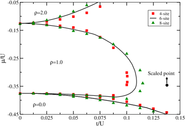
Figure 2: (Color online)Phase diagram for TCBs in both the chains for $|V|/U=−0.75$ in the $t/U$ -$\mu/U$ plane as considered in Ref. santos1 . Red squares, green up-triangles and the black solid curve represent the phase boundary for 4-, 6- and 8-sites cluster respectively. Scaled critical point for MI-SF transition $(t/U)_{c}(=0.1377)$ is shown by a solid black circle.

Before proceeding further, we first validate our CMFT method by carrying out calculations of the already existing results for a limiting case. The system of two decoupled chains, which are connected only through the non-local dipole-dipole interaction $V$, has been studied earlier using strong coupling expansion and the MPS method santos1 . It was found that the ground state phase diagram exhibits a direct MI-PSF transition as a function of $t/U$ for large values of $|V|$. Due to the attractive interaction $V$, a pairing takes place between the bosons on the two different legs of the ladder at incommensurate densities while at commensurate density, the MI phase appears in both the chains. The lower boundary of the MI lobe gets distorted with an increase in the value of $|V|$. As the strength of $|V|$ increases further, the lower Mott boundary first gets flattened out and then starts bending near the tip of the lobe. The Mott lobe in this case is distorted as a function of hopping and a re-entrant type behavior appears in the phase diagram. This behavior is also clearly visible from another calculation performed using the DMRG method danshita2 .

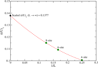
Figure 3: (Color online) Scaling of the MI-SF transition critical point $(t/U)_{c}$ with respect to the different cluster sizes at $|V|/U=−0.75$. Green solid circles represent the $(t/U)_{c}$ values for respective cluster sizes, red dashed lines represents the scaling and the black solid circle on Y-axis denotes the value of $(t/U)_{c}$ scaled to thermodynamic limit $(=0.1377)$.

To reproduce the above findings, we consider exactly the same parameters as considered in Ref. santos1 and employ the CMFT approach to obtain the MI-PSF phase boundary as shown in Fig. 2. The black solid curve shows the MI-PSF phase boundary for a six-site cluster and $|V|/U=0.75$. This already shows the bending of curvature of the lower boundary of the Mott lobe as predicted in Ref. santos1 . In order to affirm these result more distinctly we perform calculations with 8-site cluster which are shown by the green triangles. We find that the tip of the Mott lobe approaches towards the value obtained using the MPS method. Further, we perform a cluster size extrapolation to estimate the critical value $(t/U)_{c}$ at the tip of the Mott lobe as shown in Fig. 3. The extrapolated point is shown as the black filled circle in Fig. 2. The finite size extrapolation leads to $(t/U)_{c}\approx 0.14$ against the value $(t/U)_{c}\approx 0.18$, which was shown in Ref.  santos1 . The region depicted by $\rho=0$ and $\rho=2$ correspond to the empty and full states respectively. It is obvious from the above analysis that our CMFT method is able to predict the ground state of the system of TCBs reasonably well and can be used to perform a ground state analysis of the aforementioned model described by Eq. (1).

We now proceed on to discuss the main results obtained for the case, when one of the linear chains is occupied by the HCBs and the other chain by the TCBs. This situation can also mimic a two leg ladder where one leg of the ladder contains only HCBs (say, leg-a) and the other leg contains only TCBs (say, leg-b). Like previous case these bosons are also considered to be dipolar in nature and the dipole orientation is such that both the legs are coupled via attractive dipole-dipole interaction $V$ and there is no dipole-dipole interaction along the legs. In addition to this, the TCBs interact through a finite on-site interaction term $U$. Henceforth, $U$ will be used to denote the on-site two-body interaction strength for TCBs only (as for HCB, $U\rightarrow\infty$). We consider two scenarios in the following subsections. In the first case $U=0$ and in the second case we set $U\neq 0$.

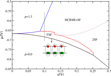
Figure 4: (Color online) Phase diagram for model given in Eq.1 in $\mu/|V|$ vs. $t/|V|$ plane, with leg-a (leg-b) containing HCB (TCB with $U=0$) with varying $t/|V|$.

III.0.1 TCBs with U=0

First we investigate the effect of an attractive $V$ on the system in the absence of two-body interaction between the TCBs, i.e. $U=0$. The detailed phase diagram for this case is shown in Fig. 4. As the on-site repulsion is absent, the bosons on different legs form a bound state of one HCB and two TCBs (HCB+2TCBs) when $|V|$ is sufficiently large compared to $t$. This happens due to the obvious reason as the two- and three-body constraints prevent more than one and two atoms on a single site of leg-a and leg-b, respectively. When the density is small, these bound state can move freely in the chains giving rise to a SF phase, which we call a trimer superfluid (TSF) phase. The TSF phase is depicted in the cartoon as the bound state of one HCB (green circle) and two TCBs (red circles). For small to moderate values of $t/|V|$, the TSF phase is always present but when $t/|V|\gtrsim 0.25$, there is a direct transition from vacuum to 2SF phase. For intermediate values of $t/|V|$, when the density of bosons and hence the value of $\mu/|V|$ increases, at some point leg-a becomes a Mott insulator with one atom in every site due to the hardcore constraint. In this limit we call this as the hardcore boson MI (HCBMI) phase. At the same time the leg-b shows a SF signature, as the trimer which was formed before can not move in the limit when the leg-a is full. We call this region of the phase diagram as the HCBMI+SF phase. Further increase in density leads to the saturation at $\rho=1.5$, i.e. $\rho=1$ and $2$ for HCBs and TCBs respectively. However, for small values of $|V|$ the system first goes to a 2SF phase from the TSF phase and then to the HCBMI+SF phase before saturating. For very large values of $|V|$ the system goes directly into the saturation from the TSF phase with increase in density of particles. In Fig. 4 , the HCBMI+SF phase is separated from the 2SF phase by the dashed line.

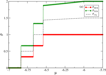
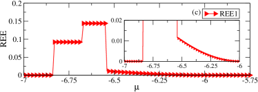
Figure 5: (Color online)(a)$\rho$ vs. $\mu$ (b)Dimer and trimer correlations and (c)Rényi entropy corresponding to a vertical cut along $U/|V|=0.0$ in Fig.8. Inset shows the zoomed in region in which REE is finite at first (HCBMI+ASF) and then gradually drops to 0 as the system approaches saturation.

To obtain the phase diagram for this case we analyze the densities and the superfluid order parameter $\phi$ of the two legs individually as well as of the whole system for different values of $t/|V|$ as a function of the chemical potential $\mu$ in a 6-site cluster (3 sites each in leg-a and leg-b). The $\rho$ vs. $\mu$ plot across a cut in the phase diagram (dashed vertical line in Fig. 4) for $t/|V|=0.1$ is shown in Fig. 5(a). In Fig. 5(a) the HCB, TCB and average density of the system are shown by red circles, green diamonds and black-dashed lines, respectively. It can be seen from this figure that there appears several discontinuous jumps in the densities as a function of $\mu$. These step-wise jumps correspond to the formation of bound states. It is to be noted that in the CMFT approach, the formation of bound states can be inferred from these discrete jumps in density for creation of every bound state. This has been confirmed in our earlier work manpreet_ladder1 . As $\mu/|V|$ increases both the legs, hence the system starts filling up. In the case of trimer formation, the filling pattern is such that for every single particle in leg-a, there are two particles in leg-b. As we go on increasing $\mu$ more particles are introduced and more such bound states are formed. This process continues until both the legs are fully occupied and the system attains its maximum possible density ($\rho=1.5$). The stepwise jump in the case of HCBs at $\rho=0.33,0.66$ and $1.0$ corresponds to 1-, 2- and 3-particle states, respectively, of the leg-a. Similarly, the stepwise jump for TCBs at $\rho=0.66,1.33$ and $2.0$ indicate 2-, 4- and 6-particle states, respectively, of leg-b. The average density of the system also behaves like wise.

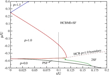
Figure 6: (Color online) Phase diagram for model given in Eq.1 in $\mu/U$ vs. $t/U$ plane, with leg-a (leg-b) containing HCB (TCB with finite two-body interaction).

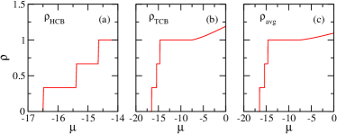
Figure 7: (Color online) $\rho$ vs. $\mu$ plot corresponding to the cut shown by dashed line across the phase diagram shown in Fig.6.

III.0.2 TCBs with U$\neq$ 0

We now discuss the situation for finite on-site two-body interaction $U$ between the TCBs. In this case the presence of on-site repulsion will play an important role as it will break the trimer phase and stabilize the MI and PSF phases. As mentioned before, in the case of soft-core bosons in both the legs it has been shown that there exists a MI-PSF phase transition as a function of $(t/U)$ for finite values of $|V|$ keeping the ratio $U/|V|=1.33$ (equitably $|V|/U=0.75$ as considered in Ref. santos1 . The PSF phase is the bound state of two bosons each from different legs. In the case of constrained bosons studied in this case, we show that the MI-PSF transition also occurs for large values of $|V|/U$. However, the phase diagram in this case shows interesting features due to the two- and three-body constraints. We vary the ratio $(t/U)$, while keeping $V$ fixed to find out the existence of various phases. The phase diagram obtained for this case is shown in Fig. 6. Compared to the previous case of TCBs with no local two-body interaction, here we do get an MI phase when the densities of both the legs becomes unity. However, before entering the MI phase the system undergoes a transition from vacuum to a PSF phase. The existence of this PSF phase can be understood with the help of $\rho$ vs. $\mu$ plot given in Fig. 7 along the dashed vertical line for $t/U=0.1$. For an attractive $V$, the system favors a bound state between the bosons of the two legs. If both the legs contain one-particle each a pair is formed. With increase in the chemical potential the number of particle in the system increases. As the system favors the formation of bound pairs, the number of particles in the system increase in steps of two particles at a time. This results in the step wise jump in the $\rho$ vs. $\mu$ plot as discussed before. The densities of HCBs, TCBs as well as the average density of the system is plotted in Fig. 7(a), (b) and (c) respectively for a 6-site cluster. The jumps in all the three plots signify the existence of the PSF phase. The plateau at $\rho=1$ corresponds to the MI phase and the shoulder above the plateau is the gapless SF phase. When the on-site interaction strength $U$ is small then the system enters into a 2SF phase with the chemical potential. However, for large values of $U$ the system favors an MI phase at commensurate density of both the legs where the density of both the legs are equal to unity. Further increasing the chemical potential leads to the HCBMI+SF phase for all values of $t/U$ as discussed in the previous section. The system saturates at $\rho_{avg}=1.5$. It is to be noted that the PSF phase, which appears along the top boundary of the MI lobe, disappears due to the hardcore constraint in one leg. This prevents the motion of the pairs once leg-a is full. As a result the bosons in leg-b can move freely in this region and hence, it is responsible for breaking the pair formation. On the other hand the re-entrant type behavior of the lower MI lobe disappears in this case owing to the fact that the hopping process for the HCBs is restricted in the MI phase and the Mott boundaries are not quadratic anymore santos1 .

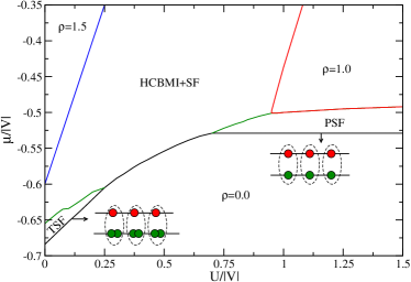
Figure 8: (Color online) Phase diagram for model given in Eq.1 in $\mu/U$ vs. $t/U$ plane, with leg-a (leg-b) containing HCB (TCB with finite two-body interaction) at $V=-10.0$.

Figure 9: (Color online) Phase diagram for model given in Eq.1 in $\mu/|V|$ vs. $U/|V|$ plane, with leg-a and leg-b containing HC and three-body constrained bosons for $t/|V|=0.03$.

After discussing two cases above it is informative to perform a careful analysis of the competition between repulsive $U$ and attractive $V$, which may reveal a more detailed phase diagram. In this regard, we explore the system by varying the $U/|V|$ ratio for a large range of values. We investigate how the phase diagram changes when the on-site interaction $U$ of TCBs in leg-b is changed for a finite value of inter-leg interaction $V$. First, we discuss the case for small $|V|$. We fix $t/|V|=0.1$ and vary $U/|V|$ to obtain the phase diagram, which is shown in Fig. 8. When $U/|V|=0$, this corresponds to the case when the system exhibits the trimer phase as discussed in the previous section. Further increase in the value of $U/|V|$ does not allow for the formation of the trimer phase as it prevents the two TCBs to occupy the same site in leg-b. Therefore, the TSF phase survives for a range of values of $U/|V|$ between $0.0$ and $0.25$. Following which we only see HCBMI+SF phase without any signature of a paired phase or the MI phase. For a relatively larger value of $U/|V|$ (beyond $U/|V|=0.75$), the density in both the legs are same. As $|V|$ is still finite, a dimer formation occurs between the legs at densities $0.33$ and $0.66$. This is indicated in the $\rho$ vs. $\mu$ plot for $U/|V|=1.0$ in Fig. 10(a). The particle number in both the legs always jumps in steps of one until the system goes to the HCBMI+ASF phase (for $0.75\lesssim U/|V|<1.0$) or the MI phase (for $U/|V|\gtrsim 1.0$).

Now we discuss the case for large $|V|$. As before, we obtain the phase diagram by varying $U/|V|$ while keeping $t/|V|=0.03$, which is shown in Fig. 9. The overall phase diagram and phases are similar as found in the previous case. A major difference is seen in the width and phase boundaries of the TSF and the PSF regions. It is seen that the TSF and PSF phase shrink and get reduced to a very small region. For intermediate values of $U/|V|(\approx 0.4-0.6)$, the repulsion between TCBs is strong enough to break the pairing in the TSF phase. In this range of $U/|V|$ there is a direct transition from vacuum to the SF phase and then to a fully occupied state. As $U/|V|$ is increased further, the system exhibits a PSF phase for incommensurate densities as $V$ is still finite and attractive in nature. At integer densities there is a transition to the MI phase in which both the HCBs and the TCBs have average densities equal to unity. When in the MI phase, as $\mu$ is increased, the TCBs drive the system first into a SF phase and eventually saturates at $\rho=1.5$.

To confirm the existence of various phase transitions discussed above we calculate correlation functions as well as the Rényi entanglement entropy (REE) of the system. We calculate the pair correlation function as

$$C_{PSF}=\langle{a_{i}}^{\dagger}{b_{i}}^{\dagger}{a_{j}}{b_{j}}\rangle,$$ (2)

and the trimer correlation function as

$$C_{TSF}=\langle{a_{i}^{\dagger}}(b_{i}^{\dagger})^{2}a_{j}(b_{j})^{2}\rangle.$$ (3)

to infer the signatures of the PSF and the TSF phases, respectively. These quantities are plotted with respect to the chemical potential $\mu$ in Fig. 5(b) and Fig. 10(b) corresponding to the cuts shown in Fig. 4 and Fig. 6, respectively. It can be seen from Fig. 5(b) that $C_{TSF}$(red triangles) clearly dominates $C_{PSF}$ in the region where the system exhibits a trimer phase as shown in Fig. 5(a). Both the correlation functions are zero in the HCBMI+SF phase. On the other hand, $C_{PSF}$ is larger than $C_{TSF}$ in the dimer phase as shown in Fig. 10(b).

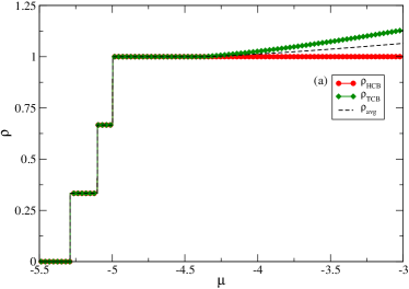
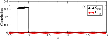
Figure 10: (Color online) (a)$\rho$ vs. $\mu$ (b)Dimer and trimer correlations and (c)Rényi entropy corresponding to a vertical cut along $U/|V|=1.0$ in Fig.8. Inset shows the zoomed in region where there is a phase transition from MI to HCBMI+SF phase and a change in slope of REE is visible.

We further calculate the REE to complement our findings in this work. This is an important quantity to probe quantum phase transitions in optical lattices which has been measured recently in an experiment on a Bose-Hubbard system greiner_2015 . The REE of $n^{th}$ order is defined as:

$$S_{n}(A)={{1}\over{1-n}}~{}log~{}Tr({\hat{\rho}_{A}}^{n})$$ (4)

where ${\hat{\rho}_{A}}$ is the reduced-density matrix of a subsystem A entangled with it’s complement B. For our calculations we focus only on the $2^{nd}$ order REE which can then be written as $S_{2}(A)=log~{}Tr({\hat{\rho}_{A}}^{2})$. The system considered can be divide into two subsystems as follows: Four left most sites can form one subsystem and the remaining (right most two sites) form another subsystem. We calculate the REE in this configuration for the cuts along $U/|V|=0.0$ and $1.0$ in the phase diagram shown in Fig. 8 and plot it as a function of $\mu$ in Fig. 5(c) and 10(c), respectively. As expected we observe finite REE in the SF, PSF and TSF phases. However in the gapped MI phase and in the saturated region, the REE reduces considerably. In Fig. 5(c), it can be seen that the REE is finite in the TSF region and as the system moves into the HCBMI+SF phase there is a significant change in REE which indicates a phase transition. As there is a contribution from SF phase REE is still finite, which can be seen in the inset of Fig. 5(c). As the system approaches saturation, REE also reduces to 0. Similar features are seen for the transition from the PSF to MI then to HCBMI+ASF phases as shown in Fig. 10(c). Our findings from the REE calculations are therefore consistent with the phase transitions indicated by the corresponding $\rho$ vs. $\mu$ and correlation function plots.

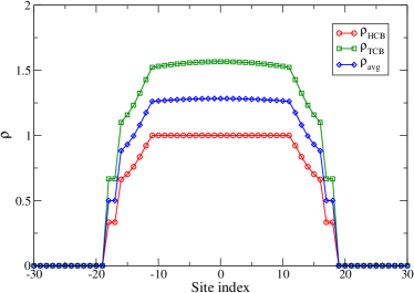
Figure 11: (Color online) HCB and TCB confined in harmonic trap with $V_{tr}=0.002$ at $U=0.0$, $t/|V|=0.225$ and $\mu/|V|=-0.6$, corresponding to Fig.4.

Here we discuss the effect of an external harmonic confinement on the quantum phase diagrams that are investigated in this work. For this purpose we consider a harmonic trap along the length of the linear chains with equal potential on both the legs and repeat the calculations. An extra term of the form $V_{tr}\sum nx^{2}$ is thus added to the system Hamiltonian, where $V_{tr}$ is the trap parameter and $x$ is the site index ($=0$ at the center). This is equivalent to redefining the effective chemical potential as $\mu_{x}=\mu_{0}-V_{tr}x^{2}$. For our calculation we set $(V_{tr}/t)=0.002$, which is experimentally achievable. The results obtained are presented in Figs. 11 and 12. In Fig. 11 we analyze the region along $t/|V|=0.225$ for $U=0.0$ and $\mu_{0}/|V|=-0.6$ of Fig. 4.

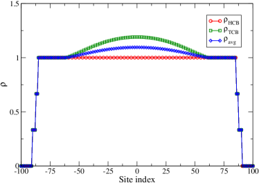
Figure 12: (Color online) HCBs and TCBs confined in harmonic trap with $V_{tr}=0.002$ at $|V|/U=0.75$, $t/U=0.1$ and $\mu/U=0.0$, corresponding to the cut shown in Fig.6.

The result is very similar to the one obtained for the homogeneous case. It is know obvious that the trap center has comparatively higher density than other sites away from the center. The center of the trap is in the HCBMI+SF phase, which can be clearly seen from the density plot in Fig. 11. Moving away from the trap center, we obtain a small region of the 2SF phase and then the TSF phase. This can be identified as the jump in the density in steps of three particles. The overall extent of all the phases is close to $40$ sites. The extent of all the phases will increase by considering a shallow trap. When we add the same trap to our system with $|V|/U=0.75$, a comparatively larger region of condensate is seen. This corresponds to a cut along $t/U=0.1$ with $\mu_{0}/U=0.0$. Once again center of the trap exhibits a HCBMI+SF phase. But unlike the previous case, we first obtain an MI phase as we move away from the center of the trap. Farther going away, it yields the PSF phase where the density changes in steps of two particles. At the trap boundaries the particle number vanishes. All these phases can be probed in the already existing technique of site resolved imaging which has been used to obtain the signature of Mott shells in the optical lattice experiments kuhr ; greiner ; kozuma .

IV Conclusions

We have studied the ground state phase diagram of two- and three-body constrained dipolar bosons in a system of two linear optical lattices coupled by the dipole-dipole interaction using the self-consistent CMFT method. We analyze a wide range of parameters and obtain phase diagrams depicting all the important phases that may arise due to the competition between the on-site two-body repulsion and the nearest neighbor attraction with the two- and three-body constraints. We find that the system exhibits mainly four types of phases; namely the 2SF, PSF, TSF and the MI phases corresponding to different ranges of parameters. We show the signature of different phases using the CMFT calculation which cannot be obtained using the conventional single site mean-field theory. By computing the pair correlation along with the trimer correlation functions, we identify the PSF and TSF phases. These results are further substantiated by the the Rényi entanglement entropy, which is found to be finite in the PSF and TSF phases and zero in the MI phase. In addition we discuss the effect of external harmonic confining potential, which emphasizes the feasibility of observing these phases in an experiment.

V Acknowledgment

We would like to thank Luis Santos and Sebastian Greschner for many useful discussions. We acknowledge DST-SERB, India for the financial support through Project No. PDF/2016/000569 and T.M. thanks IIT-Guwahati for all the financial supports through the start-up research grant. B. K. S. acknowledges financial support from CAS through the PIFI fellowship under the project number 2017VMB0023. A part of this work was carried out using Vikram-100 computing facilities at PRL, Ahmedabad and the remaining works were performed using Param-Ishan HPC facility at IIT-Guwahati.

References

- (1) I. Bloch, J. Dalibard and S. Nascimbène, Nature Physics 8, 267 (2012).
- (2) M. Lewenstein, A. Sanpera, V. Ahufinger, Ultracold Atoms in Optical Lattices, (Oxford Univ. Press), (2012).
- (3) Matthew P. A. Fisher, Peter B. Weichman, G. Grinstein, and Daniel S. Fisher, Phys. Rev. B 40, 546 (1989).
- (4) D. Jaksch, C. Bruder, J. I. Cirac, C. W. Gardiner, and P. Zoller, Phys. Rev. Lett. 81, 3108 (1998).
- (5) M. Greiner, O. Mandel, T. Esslinger, T. W. Hänsch, and I. Bloch, Nature 415, 39 (2002).
- (6) S. Will, T. Best, U. Schneider, L. Hack-ermüller, Dirk-Sören Lühmann, and I. Bloch, Nature 465, 197 (2010).
- (7) A. J. Daley and J. Simon, Phys. Rev. A 89, 053619 (2014).
- (8) P. R. Johnson, E. Tiesinga, J. V. Porto, and C. J. Williams, New J. Phys. 11, 093022 (2009).
- (9) D. S. Petrov, Phys. Rev. A 90, 021601 (2014).
- (10) A. J. Daley, J. M. Taylor, S. Diehl, M. Baranov, P. Zoller, Phys. Rev. Lett. 102, 040402 (2009).
- (11) M. Singh and T. Mishra, Phys. Rev. A 94, 063610 (2016).
- (12) M. Singh, A. Dhar, T. Mishra, R. V. Pai, and B. P. Das, Phys. Rev. A 85, 051604(R) (2012).
- (13) S. Greschner, L. Santos, and T. Vekua, Phys. Rev. A 87, 033609 (2013).
- (14) T. Lahaye, C. Menotti, L. Santos, M. Lewenstein, and T. Pfau, Rep. Prog. Phys., 72, 126401 (2009).
- (15) M. A. Baranov, M. Dalmonte, G. Pupillo, and P. Zoller, Chem. Rev. 112, 5012 (2012), and references therein.
- (16) S. Baier, M. J. Mark, D. Petter, K. Aikawa, L. Chomaz, Z. Cai, M. Baranov, P. Zoller, and F. Ferlaino, Science 352, 201 (2016).
- (17) Jun-Ru Li, J. Lee, W. Huang, S. Burchesky, B. Shteynas, F. Çaǵrı Top, A. O. Jamison, and Wolfgang Ketterle, Nature 543, 91 (2017).
- (18) F. J. Burnell, Meera M. Parish, N. R. Cooper, and S. L. Sondhi, Phys. Rev. B 80, 174519 (2009).
- (19) B. Capogrosso-Sansone, C. Trefzger, M. Lewenstein, P. Zoller, and G. Pupillo, Phys. Rev. Lett. 104, 125301 (2010).
- (20) C. Trefzger, C. Menotti, and M. Lewenstein, Phys. Rev. Lett. 103, 035304 (2009).
- (21) A. Argüelles and L. Santos, Phys. Rev. A 75, 053613 (2007).
- (22) T. Giamarchi, Quantum Physics in One Dimension, (Oxford Univ. Press), (2006).
- (23) M. A. Cazalilla, R. Citro, T. Giamarchi, E. Orignac, and M. Rigol, Reviews of Modern Physics 83, 1405 (2011).
- (24) M. S. Luthra, T. Mishra, R. V. Pai, and B. P. Das, Phys. Rev. B 78, 165104 (2008).
- (25) M. A. Cazalilla, A. F. Ho and T. Giamarchi, New J. Phys. 8, 158 (2006).
- (26) D. C. Johnston, J. W. Johnson, D. P. Goshorn, and A. J. Jacobson, Phys. Rev. B 35, 219 (1987); M. Azuma, Z. Hiroi, M. Takano, K. Ishida, and Y. Kitaoka, Phys. Rev. Lett. 73, 3463 (1994); E. Dagotto, Rep. Prog. Phys. 62, 1525 (1999); G. Vidal, Phys. Rev. Lett. 91, 147902 (2003); 93, 040502 (2004).
- (27) I. Danshita, J. E. Williams, C. A. R. Sá de Melo, and C. W. Clark, Phys. Rev. A 76, 043606 (2007).
- (28) M. Singh, T. Mishra, R. V. Pai, and B. P. Das, Phys. Rev. A 90, 013625 (2014).
- (29) M. Iskin, Phys. Rev. A 82, 055601 (2010).
- (30) E. Altman, W. Hoffstettor, E. Demler, and M. Lukin, New J. Phys. 5, 113 (2003).
- (31) A. Kuklov, N. Prokof’ev, and B. Svistunov, Phys. Rev. Lett. 92, 050402 (2004).
- (32) M. Lewenstein, L. Santos, M. A. Baranov, and H. Fehrmann, Phys. Rev. Lett. 92, 050401 (2004).
- (33) T. Mishra, Ramesh V. Pai, and B. P. Das, Phys. Rev. A 76, 013604 (2007).
- (34) T. Mishra, B. K. Sahoo, and Ramesh V. Pai, Phys. Rev. A 78, 013632 (2008).
- (35) T. Mishra, Ramesh V. Pai, and B. P. Das, Phys. Rev. B 81, 024503 (2010).
- (36) L. Mathey, Phys. Rev. B 75, 144510 (2007).
- (37) I. Titvinidze, M. Snoek, and W. Hofstetter, Phys. Rev. Lett. 100, 100401 (2008).
- (38) M. Iskin, and C. A. R. Sá de Melo, Phys. Rev. Lett. 99, 080403 (2007).
- (39) Guang-Hong Chen and Yong-Shi Wu, Phys. Rev. A 67, 013606 (2003).
- (40) F. Zhan and Ian P. McCulloch, Phys. Rev. A 89, 057601 (2014).
- (41) K. Günter, T. Stöferle, H. Moritz, M. Köhl and T. Esslinger, Phys. Rev. Lett. 96, 180402 (2006).
- (42) S. Ospelkaus et al., Phys. Rev. Lett. 96, 180403 (2006).
- (43) T. Best et al. Phys. Rev. Lett. 102, 030408 (2009).
- (44) J. Catani, L. De Sarlo, G. Barontini, F. Minardi and M. Inguscio, Phys. Rev. A 77, 011603 (2008).
- (45) B. Gadway, D. Pertot, R. Reimann, and D. Schneble, Phys. Rev. Lett. 105, 045303 (2010).
- (46) M. Taglieber, A-C. Voigt, T. Aoki,T. W. Hänsch and K. Dieckmann, Phys. Rev. Lett. 100, 010401 (2008).
- (47) S. Sugawa, K. Inaba, S. Taie, R. Yamazaki, M. Yamashita, and Y. Takahashi, Nature Physics, 7, 642, (2011).
- (48) D. Huerga, J. Dukelsky, and G. E. Scuseria, Phys. Rev. Lett. 111, 045701 (2013).
- (49) D. Yamamoto, A. Masaki, and I. Danshita, Phys. Rev. B 86, 054516 (2012).
- (50) S. R. Hassan and L. de’ Medici, Phys. Rev. B 81, 035106 (2010).
- (51) Dirk-Sören Lühmann, Phys. Rev. A 87, 043619 (2013).
- (52) S. R. White, Phys. Rev. Lett. 69, 2863 (1992).
- (53) U. Schollwöck, Rev. Mod. Phys. 77, 259 (2005).
- (54) I. Danshita, Carlos A. R. Sá de Melo, and Charles W. Clark, Phys. Rev. A 77, 063609 (2008).
- (55) R. Islam, et al, Nature 528, 77 (2015).
- (56) J. F. Sherson, C. Weitenberg, M. Endres, M. Cheneau, I. Bloch, and S. Kuhr, Nature 467, 68 (2010).
- (57) J. Simon, Waseem S. Bakr, Ruichao Ma, M. Eric Tai, Philipp M. Preiss, and M. Greiner, Nature 472, 307 (2011).
- (58) M. Miranda, R. Inoue, N. Tambo, and M. Kozuma, arXiv:1704.07060.