Nonlinear photoionization of transparent solids:
a nonperturbative theory obeying selection rules

Abstract

We provide a nonperturbative theory for photoionization of transparent solids. By applying a particular steepest-descent method, we derive analytical expressions for the photoionization rate within the two-band structure model, which consistently account for the selection rules related to the parity of the number of absorbed photons ($odd$ or $even$). We demonstrate the crucial role of the interference of the transition amplitudes (saddle-points), which in the semi-classical limit, can be interpreted in terms of interfering quantum trajectories. Keldysh’s foundational work of laser physics [Sov. Phys. JETP 20, 1307 (1965)] disregarded this interference, resulting in the violation of selection rules. We provide an improved Keldysh photoionization theory and show its excellent agreement with measurements for the frequency dependence of the two-photon absorption and nonlinear refractive index coefficients in dielectrics.

The permanent development of high-power pulsed lasers continues to attract attention to multiphoton processes, predicted by Dirac Dirac (1927) and Göppert-Mayer Göppert-Mayer (1931). Theses processes are important for a number of applications like spectroscopy Axt and Kuhn (2004); Bovensiepen and Ligges (2016), photoemission studies Damascelli et al. (2003); Pazourek et al. (2015); Bovensiepen and Ligges (2016), high harmonic generation in solids Tancogne-Dejean et al. (2017); Tamaya et al. (2016); Vampa et al. (2015, 2014); Higuchi et al. (2014), or optical communications Von Freymann et al. (2010). In particular, the spatially confined excitation produced by two-photon absorption (2PA) is useful for three-dimensional data storage and imaging Parthenopoulos and Rentzepis (1989); Denk et al. (1990); Cumpston et al. (1999). Recently, a possible way towards two-photon semiconductor lasers has been proposed Reichert et al. (2016). These successes have roused the interest in exploring applications based on three-photon absorption (3PA) He et al. (2002) and higher order multiphoton processes Zhang et al. (2014); Kerse et al. (2016).

In 1964, Leonid Keldysh developed a cornerstone theory Keldysh (1965) dedicated to multiphoton processes. While experimental data for the multiphoton absorption coefficient were favorably compared to Keldysh’s formula for the ionization probability (see Eq. (37) in Ref. Keldysh (1965)), several authors point out a discrepancy by as much as an order of magnitude, if not a lack of spectrally resolved measurements Liu et al. (1978); Nathan et al. (1985); DeSalvo et al. (1996). Moreover, experiments were conducted in the class of transparent solids with inversion symmetry allowing for one-photon transition Elliott (1957), and confirmed the frequency dependence predicted by the perturbation theory Braunstein and Ockman (1964); Vaidyanathan et al. (1980); Nathan et al. (1985) for the $l$-photon transition rate as

$$w_{l}\sim\left\{\begin{array}[]{ll}\left(l\hbar\omega-\epsilon_{g}\right)^{1/2},&l-\textrm{odd}\\ \left(l\hbar\omega-\epsilon_{g}\right)^{3/2},&l-\textrm{even}\end{array}\right.$$ (1)

where $\epsilon_{g}$ is the band-gap. In contrast, the Keldysh theory reduces to expression $w_{l}\sim\sqrt{l\hbar\omega-\epsilon_{g}}$ for $l$-odd and $l$-even Keldysh (1965), therefore violating the selection rules Vaidyanathan et al. (1980); Nathan et al. (1985). Possible reasons for this discrepancy were proposed by Vaidyanathan et al. Vaidyanathan et al. (1980), who highlighted simplifying assumptions in Keldysh’s derivation with regard to the electronic band structures and oscillator strengths. In order to achieve better agreement between theory and measurements, they suggested to replace the approximate saddle-point integration in the Keldysh derivation by an exact integration.

In this Letter, we revisit the Keldysh theory (KLD). We show that an appropriate modification of one of Keldysh’s approximations ensures that the theory, indeed, obeys the selection rules, as perturbation theory does. We perform a detailed comparison of the corrected Keldysh model (cKLD) with recent data on two-photon absorption, yielding an excellent agreement.

In Ref. Keldysh (1965), the description of the non-perturbative method to derive the expression for the photoionization rate using the Houston wave-functions Houston (1940) has been discussed in detail while features such as selection rules at low intensity Braunstein and Ockman (1964), modulation of photoionization rates with intensity caused by the dynamic Stark effect, and the calculation procedure of matrix elements have not been discussed in full detail. In order to examine the Keldysh approximations, one should draw attention to: a) matrix element approximation and b) details concerning integral calculation. In this connection we refer the reader to the recent Letters McDonald et al. (2017); Zhokhov and Zheltikov (2014) also dedicated to the approximations in Keldysh’s theory. These papers deal mostly with approximations of the band structure to unravel the difference between semiconductors and dielectrics. Here, we focus on obeying of the selection rules.

In order to proceed with the analysis, we quote Eq. (27) in Keldysh’s work Keldysh (1965) for the transition rate $w_{pi}$ from an initial state (valence band) to a final state (conduction band) due to the harmonic field $\mathcal{E}_{L}(t)=\mathcal{E}\mathrm{cos}(\omega t)$ with amplitude $\mathcal{E}$ and frequency $\omega$:

$$w_{pi}=\frac{2\pi}{\hbar}\int{\frac{\mathrm{d}\mathbf{p}}{(2\pi\hbar)^{3}}\left|\mathcal{L}_{cv}(\mathbf{p})\right|^{2}\sum_{l}{\delta(\overline{\epsilon_{cv}(\mathbf{p})}-l\hbar\omega)}},$$ (2)

where the matrix element $\mathcal{L}_{cv}$ can be defined as an integral over a closed contour $\mathcal{C}$ (enclosing the interval $(-1,1)$, see Fig. 1) in the variable $u=\mathrm{sin}\,\omega t$ (see Eq. (29), Ref. Keldysh (1965)):

$$\mathcal{L}_{cv}(\mathbf{p})=\frac{1}{2\pi}\oint_{\mathcal{C}}{\mathcal{V}_{cv}(u)e^{iS(u)}\mathrm{d}u},$$ (3)

and $S(u)$ is the classical action:

$$S(u)=\frac{1}{\hbar\omega}\int_{0}^{u}{\frac{\epsilon_{cv}(\mathbf{p}(v))}{\sqrt{1-v^{2}}}\mathrm{d}v}.$$ (4)

The presence of a large factor in the exponent in Eq. (3) allows us to calculate the integral $\mathcal{L}_{cv}$ over $u$ by a method similar to the conventional saddle-point method. Here, we unravel the key aspects of the method allowing us to calculate the PI rate consistently with the selection rules.

The saddle-points $u_{s}$ are determined by the condition $\epsilon_{cv}(\mathbf{p}(u))=0$, where the index $s:=\{\pm\}$ specifies one of the special points. However, unlike the conventional saddle-point method, the function $\epsilon_{cv}(\mathbf{p}(u))$ is not analytic and the pre-exponential factor $\mathcal{V}_{cv}(u)$ has poles at these points. The character of the singularities was considered in detail by Keldysh Keldysh (1958) and Krieger Krieger (1967). Taking these features into account, we deform the integration contour $\mathcal{C}$ with respect to $u$ as follows (see Fig. 1). We deform it from the real axis to the lower and upper half-planes so that it passes around the points $u_{s}$ along semicircles of infinitesimal small radius $r$ (via the integration paths $\mathcal{C}_{r}^{(s)}$), goes along the rays $\mathcal{C}_{s}^{(r)}$ and $\mathcal{C}_{s}^{(l)}$, where the contours $\mathcal{C}_{R}^{(r)}$ and $\mathcal{C}_{R}^{(l)}$ are used to connect the contours $\mathcal{C}^{(r)}_{s}$ and $\mathcal{C}^{(l)}_{s}$ at infinity. A simple analysis shows that the integrals $\mathcal{L}_{cv}$ along the $\mathcal{C}_{R}^{(r)}$ and $\mathcal{C}_{R}^{(l)}$ vanishes, and the integrals along the rays $\mathcal{C}_{s}^{(r)}$ and $\mathcal{C}_{s}^{(l)}$ cancel each other (for details see Supplemental Material sup ). In fact, the integration reduces to bypassing singularities with a infinitesimal small radius.

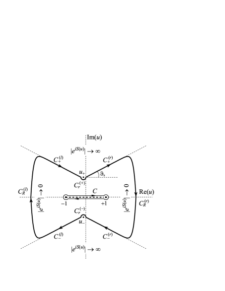
Figure 1: The integration contour for $\mathcal{L}_{cv}$ in the $u$ domain is depicted. The poles of $\mathcal{V}_{cv}$ lie at $u=u_{\pm}$ and there is a branch cut between $-1<u<+1$ on the real axis. The contours $\mathcal{C}_{R}^{(r)}$ and $\mathcal{C}_{R}^{(l)}$ are used to connect the contours $\mathcal{C}^{(r)}_{\pm}$ and $\mathcal{C}^{(l)}_{\pm}$ at infinity.

In order to evaluate the remaining integrals, we use $u=u_{s}+\xi$, and represent the function $S(u)$ in the form:

$$S(u)=\int_{0}^{u_{s}}+\int_{u_{s}}^{u_{s}+\xi}=S(u_{s})+S_{s}(\xi).$$ (5)

By expanding the pre-exponential factor in Eq. (3) near $u_{s}$, we obtain in the frame of a two-band model Keldysh (1958); Krieger (1967) for solids where one-photon transition is allowed Elliott (1957):

$$\mathcal{V}_{cv}(u)\sim\frac{\textrm{sign}(u_{s})}{4i(u-u_{s})}.$$ (6)

Thus, accounting for $\xi=u-u_{s}$, we obtain

$$\mathcal{L}_{cv}(\mathbf{p})\sim\frac{1}{4}\sum_{s}\textrm{sign}(u_{s})e^{iS(u_{s})}\int_{\mathcal{C}_{r}^{(s)}}{\frac{e^{iS_{s}(\xi)}}{\xi}\mathrm{d}\xi}.$$ (7)

In order to complete the integration in Eq. (7), the dispersion law $\epsilon_{cv}(\mathbf{p})$ must be specified. The essential difference from the Keldysh description is, however, the fact that the dispersion law must be specified at this stage rather than at stage of integration over the momentum $\mathbf{p}$ in Eq. (2). This is due to the necessity to determine the Stokes (steepest-descent) line angles. Using a certain dispersion law in $S_{s}(\xi)$ at $\mathbf{p}=0$, neglecting terms of higher order in $\xi$, and putting $\xi=r\exp(i\vartheta)$, we find that the steepest-descent lines are the rays corresponding to $\vartheta_{s}$ and $-\pi-\vartheta_{s}$. Hence, the angle between the rays determines the final contribution of each saddle-point to $\mathcal{L}_{cv}$ as follows (for details see Supplemental Material sup ):

$$\mathcal{L}_{cv}(\mathbf{p})\sim\frac{1}{4}\sum_{s}\textrm{sign}(u_{s})(\pi+2\vartheta_{s})e^{iS(u_{s})}.$$ (8)

The functions $iS(u_{s})$ in the arguments of the exponential functions in Eq. (8) and also the quasienergy $\overline{\epsilon_{cv}}$ in Eq. (2) can be calculated exactly (see Supplemental Material sup ). In result, substituting the obtained expression for $\mathcal{L}_{cv}$ in Eq. (2) and summing over the momentum, we obtain the final result for the total probability of an interband transition per unit time and per unit volume, see Eqs. (12-15) and (17-19).

Keldysh supposed Keldysh (1965) that: “the term in Eq. (36) [$iS(u_{s})$ in our notations], which is linear in $x$ [dimensionless momentum], will henceforth be left out, for when account is taken of both saddle-points it gives rise in $\mathcal{L}_{cv}$ to a rapidly oscillating factor of the type $2\mathrm{cos}(ax)$, which reduces after squaring and integrating with respect to $x$ to a factor 2, which we can take into account directly in the final answer.” However, we show that this assumption violates the selection rules (see Eq. (1)). The argument $iS(u_{s})$ of the exponential function in Eq. (8) is calculated allowing for the properties of the functions which determine it in the complex plane. Due to the summation in Eq. (8), the contribution to the integral $\mathcal{L}_{cv}$ from both saddle-points located in the complex plane acquires a phase factor (for details see Supplemental Material sup ):

$$\mathcal{L}_{cv}(\mathbf{p})\sim\left(e^{i\varphi(\mathbf{p})}-e^{-il\pi-i\varphi(\mathbf{p})}\right)\sim\sin\left(\pi l/2+\varphi\right).$$ (9)

Hence, for solids with an allowed one-photon transition, even-photon absorption is forbidden at $({l\hbar\omega-\epsilon_{g}})\,\approx\,0$ (i.e., $\varphi\,\sim\,0$), as evidenced by the perturbation theory Braunstein and Ockman (1964). Thus, the correct result is obtained via the proper treatment of the interference of the transition amplitudes and does not require an exact integration.

An interference factor of a similar nature was first obtained by Perelomov et al. Perelomov et al. (1966) in 1966 for the PI rate of atoms. However, the idea that interfering effect is important for understanding selection rules has been put forward only recently by Popruzhenko et al. Popruzhenko et al. (2002); Korneev et al. (2012) who derived a quantum equation for the PI rate and interpreted it in terms of quantum interference of scattering amplitudes using the self-consistent Born approximation and the Keldysh technique Popruzhenko et al. (2002). Our approach is based on a similar physical picture. Thus, the summation Eq. (8) can also be interpreted in terms of interfering quantum trajectories. A key feature of our approach is simplicity since matrix element can be directly evaluated the two-band model in solids, see Eq. (6).

In result, we derived a closed-form solution for the photoionization rate in transparent solids within the two-band model obeying the selection rules. The total photoionization rate per unit of volume is given by

$$w_{pi}(\omega)=\sum_{l=l_{pi}}{w^{pi}_{l}(\omega)}.$$ (10)

In the case of the Kane band structure

$$\epsilon_{cv}(\mathbf{p})=\epsilon_{g}\left(1+\frac{\mathbf{p}^{2}}{m_{r}\epsilon_{g}}\right)^{1/2},$$ (11)

the corresponding relative PI rate is of the form:

$$w_{l}^{pi}=\frac{4\omega}{9\pi}\left(\frac{m_{r}\omega}{\hbar\gamma_{2}}\right)^{3/2}Q^{K}_{l}(\gamma,x)\exp\left(-\alpha l_{pi}\right),$$ (12)

where $\alpha=\pi\left[\mathrm{K}(\gamma_{2})-\mathrm{E}(\gamma_{2})\right]/\mathrm{E}(\gamma_{1})$ and the function

$$Q_{l}^{K}(\gamma,x)=\sqrt{\frac{\pi}{2\mathrm{K}(\gamma_{1})}}\phi_{l}\left(\sqrt{\beta(l-x)}\right)\\ \times\exp\left[-\alpha\left(l-l_{pi}\right)\right],$$ (13)

varies slowly compared with an exponential function. Here, $\gamma=\omega\sqrt{m_{r}\epsilon_{g}}/(e\mathcal{E})$ is the Keldysh parameter, $\gamma_{1}=(1+\gamma^{2})^{-1/2}$, $\gamma_{2}=\gamma(1+\gamma^{2})^{-1/2}$, $\beta=\pi^{2}/\left[2\mathrm{K}(\gamma_{1})\mathrm{E}(\gamma_{1})\right]$, $\epsilon_{g}$ is the energy gap, $x=\bar{\epsilon}_{g}/\hbar\omega$, $\bar{\epsilon}_{g}=2\epsilon_{g}\mathrm{E}(\gamma_{1})/(\pi\gamma_{2})$, $l_{pi}=[x+1]$ (where the symbol [$x$] denotes the integer part of a number $x$), the functions $\mathrm{K}$ and $\mathrm{E}$ are the complete elliptic integrals of the first and second kind, and the function $\phi_{l}$ is

$$\phi_{l}(z)=e^{-z^{2}}\int_{0}^{z}\sin^{2}\left(\frac{\pi l}{2}+ay\right)e^{y^{2}}\mathrm{d}y,$$ (14)

and

$$a=\sqrt{\frac{\epsilon_{g}\mathrm{K}(\gamma_{1})}{2\pi\hbar\omega\gamma_{2}}}\operatorname{arccot}\left(\frac{1}{2\gamma}-\frac{\gamma}{2}\right).$$ (15)

In the case of a parabolic band structure

$$\epsilon_{cv}(\mathbf{p})=\epsilon_{g}\left(1+\frac{\mathbf{p}^{2}}{2m_{r}\epsilon_{g}}\right),$$ (16)

the total PI rate is also given by Eq. (10) and the corresponding relative PI rate is of the form:

$$w_{l}^{pi}=\frac{\omega}{4\pi}\left(\frac{m_{r}\omega}{\hbar}\right)^{3/2}Q_{l}^{P}(\gamma,x)\exp\left(-\hat{\alpha}l_{pi}-\Theta x\right),$$ (17)

where $\hat{\alpha}=\left[2\sinh^{-1}(\sqrt{2}\gamma)-\hat{\beta}\right]$, $\hat{\beta}=2/\sqrt{1+1/2\gamma^{2}}$, $\Theta=2\hat{\beta}\gamma^{2}/(1+4\gamma^{2})$, $\bar{\epsilon}_{g}=\epsilon_{g}\left[1+{1}/({4\gamma^{2}})\right]$, and

$$Q_{l}^{P}(\gamma,x)=\sqrt{\frac{2}{\hat{\beta}}}\phi_{l}\left(\sqrt{\hat{\beta}(l-x)}\right)\exp\left[-\hat{\alpha}\left(l-l_{pi}\right)\right]$$ (18)

and the function $\phi_{l}$ is the same as in Eq. (14) with

$$a=\sqrt{\frac{2\epsilon_{g}}{\hbar\omega\hat{\beta}}}\left(-\frac{1}{\gamma}+\frac{2\sqrt{2}}{\hat{\beta}}\right).$$ (19)

A simple analysis shows that the rates, Eqs. (12) and (17), are reduced to Eq. (1) via a small z-expansion of $\phi_{l}$:

$$\phi_{l}\sim\left\{\begin{array}[]{ll}\left(l\hbar\omega-\bar{\epsilon}_{g}\right)^{1/2}&,\leavevmode\nobreak\ l-\textrm{odd}\\ \left(l\hbar\omega-\bar{\epsilon}_{g}\right)^{3/2}&,\leavevmode\nobreak\ l-\textrm{even}\end{array}\right.$$ (20)

i.e., obey the selection rules for any band structure approximation, Kane or parabolic, hence, agree with the perturbation theory at low intensities ($\gamma\gg 1$).

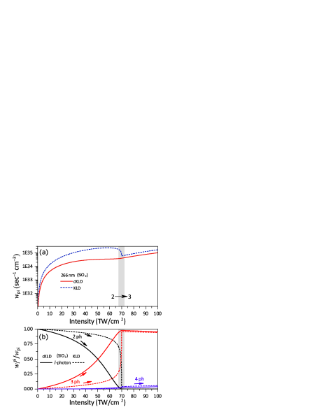
Figure 2: Comparison between the original Keldysh and the corrected Keldysh formulas of photoionization rates as functions of laser intensity at 266 nm wavelength in SiO₂. Solid curves correspond to cKLD formula and dashed curves reproduce the KLD formula. (a) Total PI rate. (b) Relative contribution of 2- (black), 3- (red) and 4-photon (blue) processes to photoionization. The channel-closure region at $I\approx 70$ TW cm^-2 is indicated by the grey shaded area, (a) and (b), and horizontal arrow, (a). Note: com .

Figure 3: Comparison between theory (curves) and experiment (markers) in SiO₂ (blue) and Al₂O₃ (purple). Solid and dashed curves are numerical results via cKLD and KLD theory, respectively. (a) 2PA coefficient $\beta_{2}$. Fused silica (empty circles) and crystalline quartz (filled circles) Dragonmir et al. (2002); Slattery and Nikogosyan (2003), Al₂O₃ Leedle et al. (2017) (empty squares) and DeSalvo et al. (1996) (filled square). (b) Experimental and numerical nonlinear refractivity index $n_{2}$. Experimental data are taken from DeSalvo et al. (1996): empty circles for SiO₂ and empty squares for Al₂O₃. Notes: com ; rem .

In order to compare the results of the corrected theory with experiment, we choose SiO₂ and Al₂O₃, two highly relevant materials for industrial applications. The band structure of these wide-band gap insulators Waroquiers et al. (2013); French (1990) can be well approximated by a two-band model with only two parameters, the reduced mass $m_{r}$ and the band gap $\epsilon_{g}$. We use $m_{r}=0.9\leavevmode\nobreak\ m_{0}$ and $\epsilon_{g}=9.0$ eV for SiO₂, and $m_{r}=0.35\leavevmode\nobreak\ m_{0}$ and $\epsilon_{g}=8.8$ eV for Al₂O₃.

Fig. 2(a) shows the dependence of the PI rate per unit volume on laser intensity, for SiO₂ at the laser wavelength 266 nm, as calculated from the KLD theory and the cKLD model. The cusp at $\approx 70$ TW/cm² is the signature of 2PA to 3PA transition in the Keldysh formula, and is due to the energy shortage as the electron ponderomotive energy grows up with increasing laser field amplitude (the dynamic Stark effect), and thus, the probability of photoionization decreases sharply highlighting the signature of channel-closing Paulus et al. (2001); Zimmermann et al. (2017). As can be seen in Fig. 2(a), this cusp is no longer present in our corrected cKLD model reflecting the proper superposition of channels, 2PA and 3PA, respectively. In Fig. 2(b) we evaluate the relative contribution of multi-photon processes (channels) to the total photoionization rate. For the KLD model, the contribution of 2PA vanishes at $\approx 70$ TW/cm², i.e. the channel closes, while the contribution of 3PA abruptly increases. For the cKLD model, a smooth transition from 2PA to 3PA is obtained: the contribution of 3PA compensates for the attenuation of the 2PA process.

By taking into consideration only the 2PA process, that is valid in the limit of low laser intensities, we compare theoretical predictions for the 2PA coefficient $\beta_{2}$ calculated from the KLD and cKLD models with measurements for SiO₂ Dragonmir et al. (2002); Slattery and Nikogosyan (2003) and recent data for Al₂O₃ Leedle et al. (2017), see Fig. 3(a). The improved Keldysh model, cKLD matches better with the experimental findings, especially, in the vicinity of the transition from 2PA to 3PA ($\hbar\omega/\epsilon_{g}\approx 0.5$), where the Keldysh model overestimates the absorption rate by a factor of $\sim 10$, and further highlights and confirms the selection rules signature. The application of the Kramers-Kronig relation to the imaginary part of the permittivity gives the frequency dependence of the complex dielectric function $\varepsilon(\omega)=\varepsilon_{r}(\omega)+i\varepsilon_{i}(\omega)$, and thus, allowing as to derive the dispersion curves of the nonlinear refractive index $n_{2}(\omega)$:

$$n_{2}(\omega)I=\operatorname{Re}\left(\sqrt{\varepsilon(\omega)}\right)-n_{0}(\omega),$$

where $n_{0}(\omega)$ is the linear index approximated by three-term Sellmeier dispersion equation for SiO₂ Malitson (1965), Al₂O₃ Malitson (1962), and $I=\epsilon_{0}cn_{0}\mathcal{E}^{2}/2$ is the laser intensity in the bulk. Dispersion curves $n_{2}$ are shown in Fig. 3(b), where we present the comparison of the cKLD and KLD models with measurements DeSalvo et al. (1996), demonstrating again excellent agreement. As can be seen, both models give similar behaviour except for the sharp peak (resonance-like behaviour) at half the band gap energy, where Keldysh’s model exhibits a cusp originating from the omission discussed above, whereas the corrected model yields a significant improvement.

In this Letter we revise the Keldysh approximations and reveal that after the appropriate correction the Keldysh theory indeed obeys the selection rules and reduces to the equivalent results of perturbation theory. We also demonstrate that the selection rules can be understood as a classical effect caused by interference of quantum trajectories. In order to remedy the Keldysh omission, we propose a simple correction taking into account such interfering effect. The results yield excellent agreement with experimental measurements of the two-photon absorption coefficient $\beta_{2}$ as well as nonlinear refractive index $n_{2}$ for materials Al₂O₃ and SiO₂.

The authors thank S. Popruzhenko and N. Shvetsov-Shilovski for useful discussions. MEP acknowledges support of the CNRS. NSS and MEP are grateful to the Russian Foundation for Basic Research (project No. 16-02-00266) for financial support.

References

- Dirac (1927) P. A. M. Dirac, Proc. R. Soc. A 114, 710 (1927).
- Göppert-Mayer (1931) M. Göppert-Mayer, Ann. Phys. (Berlin) 401, 273 (1931).
- Axt and Kuhn (2004) V. M. Axt and T. Kuhn, Rep. Prog. Phys. 67, 433 (2004).
- Bovensiepen and Ligges (2016) U. Bovensiepen and M. Ligges, Science 353, 28 (2016).
- Damascelli et al. (2003) A. Damascelli, Z. Hussain, and Z.-X. Shen, Rev. Mod. Phys. 75, 473 (2003).
- Pazourek et al. (2015) R. Pazourek, S. Nagele, and J. Burgdörfer, Rev. Mod. Phys. 87, 765 (2015).
- Tancogne-Dejean et al. (2017) N. Tancogne-Dejean, O. D. Mücke, F. X. Kärtner, and A. Rubio, Phys. Rev. Lett. 118, 087403 (2017).
- Tamaya et al. (2016) T. Tamaya, A. Ishikawa, T. Ogawa, and K. Tanaka, Phys. Rev. Lett. 116, 016601 (2016).
- Vampa et al. (2015) G. Vampa, T. Hammond, N. Thiré, B. Schmidt, F. Légaré, C. McDonald, T. Brabec, and P. Corkum, Nature 522, 462 (2015).
- Vampa et al. (2014) G. Vampa, C. R. McDonald, G. Orlando, D. D. Klug, P. B. Corkum, and T. Brabec, Phys. Rev. Lett. 113, 073901 (2014).
- Higuchi et al. (2014) T. Higuchi, M. I. Stockman, and P. Hommelhoff, Phys. Rev. Lett. 113, 213901 (2014).
- Von Freymann et al. (2010) G. Von Freymann, A. Ledermann, M. Thiel, I. Staude, S. Essig, K. Busch, and M. Wegener, Adv. Func. Mat. 20, 1038 (2010).
- Parthenopoulos and Rentzepis (1989) D. A. Parthenopoulos and P. M. Rentzepis, Science 245, 843 (1989).
- Denk et al. (1990) W. Denk, J. H. Strickler, and W. W. Webb, Science 248, 73 (1990).
- Cumpston et al. (1999) B. H. Cumpston, S. P. Ananthavel, S. Barlow, D. L. Dyer, J. E. Ehrlich, L. L. Erskine, A. A. Heikal, S. M. Kuebler, I.-Y. S. Lee, D. McCord-Maughon, et al., Nature 398, 51 (1999).
- Reichert et al. (2016) M. Reichert, A. L. Smirl, G. Salamo, D. J. Hagan, and E. W. Van Stryland, Phys. Rev. Lett. 117, 073602 (2016).
- He et al. (2002) G. S. He, P. P. Markowicz, T.-C. Lin, and P. N. Prasad, Nature 415, 767 (2002).
- Zhang et al. (2014) J. Zhang, M. Gecevičius, M. Beresna, and P. G. Kazansky, Phys. Rev. Lett. 112, 033901 (2014).
- Kerse et al. (2016) C. Kerse, H. Kalaycıoğlu, P. Elahi, B. Çetin, D. K. Kesim, Ö. Akçaalan, S. Yavaş, M. D. Aşık, B. Öktem, H. Hoogland, et al., Nature 537, 84 (2016).
- Keldysh (1965) L. V. Keldysh, Sov. Phys. JETP 20, 1307 (1965), [J. Exptl. Theoret. Phys. (U.S.S.R.) 47, 1945 (1964)].
- Liu et al. (1978) P. Liu, W. L. Smith, H. Lotem, J. H. Bechtel, N. Bloembergen, and R. S. Adhav, Phys. Rev. B 17, 4620 (1978).
- Nathan et al. (1985) V. Nathan, A. H. Guenther, and S. S. Mitra, JOSA B 2, 294 (1985).
- DeSalvo et al. (1996) R. DeSalvo, A. A. Said, D. J. Hagan, E. W. Van Stryland, and M. Sheik-Bahae, IEEE J. Quant. Electr. 32, 1324 (1996).
- Elliott (1957) R. J. Elliott, Phys. Rev. 108, 1384 (1957).
- Braunstein and Ockman (1964) R. Braunstein and N. Ockman, Phys. Rev. 134, A499 (1964).
- Vaidyanathan et al. (1980) A. Vaidyanathan, T. Walker, A. H. Guenther, S. S. Mitra, and L. M. Narducci, Phys. Rev. B 21, 743 (1980).
- Houston (1940) W. V. Houston, Phys. Rev. 57, 184 (1940).
- McDonald et al. (2017) C. R. McDonald, G. Vampa, P. B. Corkum, and T. Brabec, Phys. Rev. Lett. 118, 173601 (2017).
- Zhokhov and Zheltikov (2014) P. A. Zhokhov and A. M. Zheltikov, Phys. Rev. Lett. 113, 133903 (2014).
- Keldysh (1958) L. V. Keldysh, Sov. Phys. JETP 6, 763 (1958), [J. Exptl. Theoret. Phys. (U.S.S.R.) 34, 962–968 (1957)].
- Krieger (1967) J. B. Krieger, Phys. Rev. 156, 776 (1967).
- (32) See Supplemental Material at http://link.aps.org/supplemental/.
- Perelomov et al. (1966) A. M. Perelomov, V. S. Popov, and M. V. Terent’ev, Sov. Phys. JETP 23, 924 (1966), [J. Exptl. Theoret. Phys. (U.S.S.R.) 50, 1393 (1966)].
- Popruzhenko et al. (2002) S. V. Popruzhenko, P. A. Korneev, S. P. Goreslavski, and W. Becker, Phys. Rev. Lett. 89, 023001 (2002).
- Korneev et al. (2012) P. A. Korneev, S. V. Popruzhenko, S. P. Goreslavski, T.-M. Yan, D. Bauer, W. Becker, M. Kübel, M. F. Kling, C. Rödel, M. Wünsche, and G. G. Paulus, Phys. Rev. Lett. 108, 223601 (2012).
- (36) The electron spin is taken into account.
- Dragonmir et al. (2002) A. Dragonmir, J. G. McInerney, and D. N. Nikogosyan, Appl. Opt. 41, 4365 (2002).
- Slattery and Nikogosyan (2003) S. A. Slattery and D. N. Nikogosyan, Opt. Comm. 228, 127 (2003).
- Leedle et al. (2017) K. J. Leedle, K. E. Urbanek, and R. L. Byer, Appl. Opt. 56, 2226 (2017).
- (40) Sapphire 2PA coefficient measured via z-scan technique DeSalvo et al. (1996) at (filled square) is roughly one order of magnitude above the values obtained via two-photon conductive sapphire sensor Leedle et al. (2017) (empty squares) at , that is explained by “possible reduction in the measured current extraction due to carrier recombination”.
- Waroquiers et al. (2013) D. Waroquiers, A. Lherbier, A. Miglio, M. Stankovski, S. Poncé, M. J. T. Oliveira, M. Giantomassi, G.-M. Rignanese, and X. Gonze, Phys. Rev. B 87, 075121 (2013).
- French (1990) R. H. French, J. Am. Ceram. Soc. 73, 477 (1990).
- Paulus et al. (2001) G. G. Paulus, F. Grasbon, H. Walther, R. Kopold, and W. Becker, Phys. Rev. A 64, 021401 (2001).
- Zimmermann et al. (2017) H. Zimmermann, S. Patchkovskii, M. Ivanov, and U. Eichmann, Phys. Rev. Lett. 118, 013003 (2017).
- Malitson (1965) I. H. Malitson, JOSA 55, 1205 (1965).
- Malitson (1962) I. H. Malitson, JOSA 52, 1377 (1962).