Theory of the spin galvanic effect at oxide interfaces

Abstract

The spin galvanic effect (SGE) describes the conversion of a non-equilibrium spin polarization into a transverse charge current. Recent experiments have demonstrated a large conversion efficiency for the two-dimensional electron gas formed at the interface between two insulating oxides, LaAlO₃ and SrTiO₃. Here we analyze the SGE for oxide interfaces within a three-band model for the Ti t_2g orbitals which displays an interesting variety of effective spin-orbit couplings in the individual bands that contribute differently to the spin-charge conversion. Our analytical approach is supplemented by a numerical treatment where we also investigate the influence of disorder and temperature, which turns out to be crucial to provide an appropriate description of the experimental data.

The spin galvanic effect (SGE) is the generation of an electrical current by a non-equilibrium spin density. The latter may be obtained by optical or magnetic pumping. There exists also the inverse effect (ISGE) by which the spin of free carriers can be oriented by an applied electric field. The SGE effect was first predicted [1] and then observed for Te crystals [2]. About a decade later, the SGE was studied theoretically [3, 4, 5] in the two-dimensional electron gas (2DEG) in the presence of Rashba spin-orbit coupling (SOC) arising from the asymmetry of the quantum well [6]. The effect was later observed in quantum wells by absorption of polarized light [7, 8, 9]. Whereas at microscopic level the coupling between the spin polarization and the electrical current is provided by the SOC, the origin of the effect rests on the restricted symmetry conditions of gyrotropic media, where polar and axial vectors transform according to the same representation (c.f. the review by Ganichev et al., [10]). The conditions of sizable SOC and lack of inversion symmetry can be obtained also in other physical systems. Recently, indeed, the SGE has been observed at a silver-bismuth interface where the non-equilibrium spin polarization has been pumped by an adjacent ferromagnetic layer with a precessing magnetization [11]. Magnetic spin pumping was successively used to observe the SGE in a number of different interface systems as in ferromagnetic-topological insulators [12, 13] and ferromagnetic-oxide systems [14, 15, 16]. In the latter case, the oxide being a heterostructure of LaAlO₃ (LAO) and SrTiO₃ (STO), the complex band structure originating from the Ti orbitals may lead to a richer phenomenology [17, 18], as compared to other systems where the standard continuum 2DEG model with spin-orbit split bands provides a good quantitative and qualitative understanding of the effect. Indeed, the spin-polarization induced transverse voltage $V_{SGE}$ can be modulated by gating the heterostructure which changes the chemical potential $\mu$, i.e. the carrier density in the 2D interface layer. Quite dramatically, a sign change occurs [15] in $V_{SGE}$ at a particular value of $\mu$, and has been attributed to a Lifshitz transition, where the $d_{xz}$, $d_{yz}$ bands originating from the Ti $t_{2g}$ orbitals start to be filled. Moreover, the effect strongly depends on temperature and on the number of LAO layers in the LAO/STO heterostructure [16].

In Fig. 1 a) we sketch the physical origin of the ISGE in a 2DEG with standard parabolic spectrum. In the presence of an applied electric field $E_{x}$ along the $x$ direction, the distribution function is shifted in momentum space by an amount $\delta k_{x}=-eE_{x}\tau$, where $e>0$ is the unit charge and $\tau$ the elastic scattering time. In the presence of Rashba SOC [6], $H_{RSOC}=\alpha\hbar(\tau_{x}k_{y}-\tau_{y}k_{x})$ with $\tau_{i}$ denoting the Pauli matrices, each momentum state sees an effective magnetic field (blue thin arrows) perpendicular to the momentum, see Fig. 1 a). The presence of the electric field adds up a non-equilibrium magnetic field directed along the negative $y$ axis. As a result the magnetic field (light blue tick arrows) seen at each momentum state is no longer just opposite for $k_{x}$ and $-k_{x}$ states. This difference in magnetic field, which is linear in the SOC constant $\alpha$, leads to a net spin polarization along the $y$ axis, $S_{y}=\sigma^{ISGE}E_{x}$ [4], where $\sigma^{ISGE}=-e\alpha N_{0}\tau$ denotes the inverse spin galvanic response and $N_{0}$ is the two-dimensional density of states (DOS) per spin of the parabolic band. Hence, the sign of the ISGE and, by Onsager reciprocity arguments, that of the SGE $\sigma^{SGE}$, is a direct consequence of the sign of the Rashba SOC. Because both the spin polarization $S_{y}$ and the charge current $J_{x}$ are odd under time reversal, SGE and ISGE are the same, thus sharing the same sign.

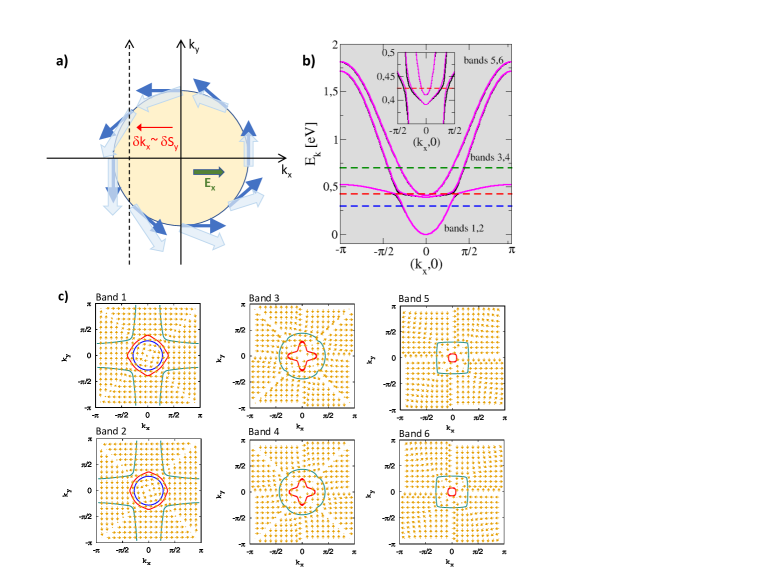
Figure 1: a) Schematic physical picture of the origin of the ISGE. b) Structure of the $t_{2g}$ interface bands. The inset enlarges the region around the Lifshitz point where the spin-orbit splitting is large. The horizontal dashed lines in the main panel refer to the chemical potentials $\mu=0.3$ eV (blue), $\mu=0.425$ eV (red) and $\mu=0.7$ eV (green). c) The chiral spin structure for the upper band of each of the three pair of bands together with the Fermi surface. For the lower bands the spins point in the opposite direction.

In this letter we provide the theory of the SGE and ISGE for the 2DEG at the LAO/STO interface. As it is customary [19, 20, 21], the latter is described by a tight-binding model of the Ti t_2g orbitals supplemented by atomic spin-orbit interactions and an inter-orbital hopping induced by the interface asymmetry. Our aim is to understand what are the peculiar features of the SGE in an effectively six-band model (the $d_{xy}$, $d_{xz}$ and $d_{yz}$ orbitals with the additional spin degree of freedom) and to what extent it can be described in terms of the concepts developed for the Rashba SOC in the 2DEG in semiconductor quantum wells. More specifically, we address the question whether the sign of the SGE can be related to the orientation of the internal magnetic field with respect to the momentum. To this end we use a numerical technique, which allows us to evaluate exactly, in a finite system, the Kubo formula for the spin density-charge current response function [22]. Close to the $\Gamma$ point in momentum space, the tight-binding band structure can be approximated by a continuum model, which can be tackled analytically by means of standard quantum-field theory techniques normally employed in the study of disordered electron systems. This allows us to develop a picture of the sign behavior of the SGE as a function of the position of the chemical potential in the band structure.

The tight-binding Hamiltonian is composed of three parts

$$H=H_{0}+H_{aso}+H_{I},$$ (1)

describing the tight-binding hopping of the Ti t_2g orbitals, the atomic SOC and the inter-orbital hopping, respectively. The first term, $H_{0}$, is diagonal in the basis $(|xy\rangle\otimes|\sigma\rangle,\ |xz\rangle\otimes|\sigma\rangle,\ |yz\rangle\otimes|\sigma\rangle)$, $\sigma=\uparrow,\downarrow$, with spin-degenerate energies

$$\varepsilon^{xy}_{k} = -2t_{1}[\cos(k_{x})+\cos(k_{y})-2]$$

$$-4t_{3}[\cos(k_{x})\cos(k_{y})-1],$$

$$\varepsilon^{xz}_{k} = -2(t_{1}+t_{3})[\cos(k_{x})-1]-2t_{2}[\cos(k_{y})-1]+\Delta,$$

$$\varepsilon^{yz}_{k} = -2(t_{1}+t_{3})[\cos(k_{y})-1]-2t_{2}[\cos(k_{x})-1]+\Delta,$$

where the energy difference $\Delta$ between $|xy\rangle$ and $|xz\rangle,|yz\rangle$ states is due to the confinement of the 2DEG near the interfacial $xy$-plane. The standard ${\bf l}\cdot{\bf s}$ coupling leads to the atomic SOC Hamiltonian

$$H_{aso}=\Delta_{aso}\left(\begin{array}[]{ccc}0&-i\tau_{x}&i\tau_{y}\\ i\tau_{x}&0&-i\tau_{z}\\ -i\tau_{y}&i\tau_{z}&0\end{array}\right).$$

Finally, the crystal symmetry is lifted at the interface and the orbitals get coupled through the spin independent Hamiltonian

$$H_{I}=\gamma\left(\begin{array}[]{ccc}0&-2i\sin(k_{y})&-2i\sin(k_{x})\\ 2i\sin(k_{y})&0&0\\ 2i\sin(k_{x})&0&0\end{array}\right)\,.$$

In Fig. 1 b) we plot the band structure of the Hamiltonian of Eq. (1), with $t_{1}=0.277$ eV, $t_{2}=0.031$ eV, $t_{3}=0.076$ eV, $\Delta=0.4$ eV, $\Delta_{aso}=0.01$ eV, $\gamma=0.02$ eV, as derived in Ref. [19] from projecting DFT on the $t_{2g}$ Wannier states [23]. Bands come in spin-orbit split pairs indicated by black and magenta curves. The pair of bands 1 and 2 originates mostly from the $d_{xy}$ orbital, whereas pairs 3,4 and 5,6 from the mixing of $d_{xz}$ and $d_{yz}$ due to the interface asymmetry term in the Hamiltonian. The horizontal dashed lines (red, blue and green) show different positions of the Fermi level in the bands. In the Rashba Hamiltonian, the eigenstates at fixed momentum ${\bf k}$ form a Kramers doublet with opposite helicity, defined as the spin projection along the quantization axis, which is perpendicular to the momentum. In Fig. 1 c) we show the vector plots of the chiral spin structure for the three pairs of bands. As we will show, the analysis of the behavior of the helicity of the band eigenstates provides a useful guide to understand the origin of the sign of the SGE obtained by a quantitative calculation.

Let us concentrate first on the lowest pair of bands (1,2). At low electron filling, the Fermi surface is circular (cf. the blue line in the first column of panel c in Fig. 1). The helicity of the two spin-split bands is opposite and close to $\Gamma$ is given by $\Lambda\sim{\vec{S}_{12}}\sim s\,{\vec{e}_{\phi}}$, where ${\vec{e}_{\phi}}$ denotes the tangential unit vector $(-\sin(\phi),\cos(\phi))$ and here and in the following $s=\mp$ refers to the lower (1,3,5) and upper (2,4,6) of each pair of bands, respectively. The structure therefore resembles that of the Rashba model but for an overall sign. Indeed, expansion near the $\Gamma$ point [21, 24] leads to an effective Hamiltonian $H_{12}=\alpha_{xy}(k_{y}\tau_{x}-k_{x}\tau_{y})$ for the (1,2) two bands, i.e. to a Rashba Hamiltonian with a negative coupling constant $\alpha_{xy}=-4\gamma\Delta_{aso}/\Delta$. By increasing the filling, the Fermi surface acquires a distortion compatible with the crystal symmetry, which for the Rashba Hamiltonian is ruled by the $C_{4v}$ point group. However, the overall sign behavior of the helicity does not change. For bands (3,4) the effective Hamiltonian close to $\Gamma$ reads $H_{34}=-\beta(k_{x}^{2}-k_{y}^{2})(\tau_{x}k_{y}-\tau_{y}k_{x})$ with $\beta=\gamma(t_{1}+t_{3}-t_{2})/\Delta$, i.e. a Rashba-like Hamiltonian with a momentum-dependent coupling $\sim-\beta(k_{x}^{2}-k_{y}^{2})$. At first sight, it seems that the factor $k_{x}^{2}-k_{y}^{2}$ spoils the $C_{4v}$ symmetry. This can be seen by noticing that under a $\pi/4$-rotation, Pauli matrices and momentum components transform as $\tau_{x}\rightarrow\tau_{y},\tau_{y}\rightarrow-\tau_{x}$ and $k_{x}\rightarrow k_{y},k_{y}\rightarrow-k_{x}$. Such a violation of symmetry does not occur, though, because the spin operator for the $S_{y}$ polarization, when projected onto the sector of the (3,4) bands, becomes $S_{y}=-\kappa(k_{x}^{2}-k_{y}^{2})\tau_{y}/2$ with $\kappa=(t_{1}+t_{3}-t_{2})/(4\Delta_{aso})$, thus restoring the correct symmetry at the level of physical observables. Including the additional prefactor from the spin projection therefore yields a helical spin structure close to $\Gamma$ ${\vec{S}_{34}}\sim-s|\cos(2\phi)|{\vec{e}_{\phi}}\sim-|\cos(2\phi)|{\vec{S}_{12}}$, i.e. a helicity opposite to that of bands 1(2). Finally, in the case of bands (5,6), the effective Hamiltonian at low filling reads $H_{56}=\alpha(\tau_{x}k_{y}+\tau_{y}k_{x})$ with $\alpha=4\gamma\Delta_{aso}/\Delta$. Even in this case, as for the bands (3,4), the form of the Hamiltonian appears to violate the $C_{4v}$ symmetry and in fact is Dresselhaus-like and obeys the $D_{2d}$ symmetry. However, also in this case the correct spin operator in the restricted basis is $S_{y}=\kappa(k_{x}^{2}-k_{y}^{2})\tau_{y}/2$ and restores the $C_{4v}$ symmetry. The helical spin structure near $\Gamma$, ${\vec{S}_{56}}\sim s\cos(2\phi)\tau_{z}{\vec{e}_{\phi}}\sim-\cos(2\phi)\tau_{z}{\vec{S}_{12}}$, has a helicity which is opposite to that of the pair (3,4).

As outlined above in the diffusive limit the sign of the spin galvanic response for the Rashba model is intimately connected to the sign of the SOC and thus to the helicity of the bands. Table 1 summarizes the argument by providing in the 5th row the result for the spin galvanic response obtained in the diffusive limit in the vicinity of the $\Gamma$ point by using standard field-theory impurity techniques. Clearly, the helicity $\Lambda$ for each pair of bands determines the sign of $\sigma^{SGE}$ which in Tab. 1 is given in terms of the Fermi momentum $p_{F}$ and the coupling constants defined above. Close to the $\Gamma$ point the bands, in the absence of SOC, are parabolic with a circular Fermi surface of radius $p_{F}$. From this analysis we therefore may expect a sign change in $\sigma^{SGE}$ upon going from bands (1,2) to bands (3,4) and a further sign change upon shifting the chemical potential into the bottom of bands (5,6). As already mentioned, Onsager reciprocity $\sigma^{ISGE}=\sigma^{SGE}$ implies the same result for the inverse SGE.

However, while the above reasoning provides a detailed understanding of the SGE in the individual bands the total response involves the sum of these intraband contributions and, moreover, is expected also to depend on scattering processes between the bands, in particular close to the Lifshitz point.

(r,0.3cm,0.4cm)[4pt]—c—c—c—c——c—c—c—c—c—c— Bands & $(1,2)$ $(3,4)$ $(5,6)$
$H$ $-\alpha(\tau_{x}k_{y}-\tau_{y}k_{x})$ $-\beta(k_{x}^{2}-k_{y}^{2})(\tau_{x}k_{y}-\tau_{y}k_{x})$ $\alpha(\tau_{x}k_{y}+\tau_{y}k_{x})$
$S^{y}$ $\tau_{y}/2$ $-\kappa(k_{x}^{2}-k_{y}^{2})\tau_{y}/2$ $\kappa(k_{x}^{2}-k_{y}^{2})\tau_{y}/2$
$\Lambda$ $-/+$ $+/-$ $-/+$
$\sigma^{SGE}$ $(-e)N_{0}\tau(-\alpha)$ $(-e)N_{0}\tau(\beta p_{F}^{2})(\kappa p_{F}^{2})\frac{5}{8}$ $(-e)N_{0}\tau(-\alpha)(\kappa p_{F}^{2})$
$D^{SGE}$ $(-e)N_{0}\pi\left(-\alpha\right)\frac{1}{2}$ $(-e)N_{0}\pi(\beta p_{F}^{2})(\kappa p_{F}^{2})\frac{1}{4}$ $(-e)N_{0}\pi\alpha(\kappa p_{F}^{2})\frac{1}{4}$

Table 1: Effective Hamiltonian for the three pairs of bands close to the $\Gamma$ point, together with the form of the spin polarization operator $S_{y}$ and the resulting helicities $\Lambda$. In the absence of disorder, when the scattering time $\tau\rightarrow\infty$, the SGE response has a Drude-like peak with weight $D^{SGE}$ as for the longitudinal conductivity. In the presence of disorder, the Drude-like peak evolves in the DC limit value of the SGE coefficient $\sigma^{SGE}$.

In the remaining of this paper, we are going to discuss these important effects by a means of exact numerical evaluation of the Kubo formula for the conductivity $\chi^{SGE}(\omega)=\langle\langle J_{x};S^{y}\rangle\rangle_{\omega}/[i(\omega+i\eta)]$, with

$$\langle\langle J_{x};S^{y}\rangle\rangle_{\omega}=\frac{1}{N}\sum_{k,p}(f_{p}-f_{k})\frac{\langle p|S^{y}|k\rangle\langle k|J_{x}|p\rangle}{\omega+i\eta+E_{p}-E_{k}},$$

where $J_{x}$ is the total charge current (obtained from the usual Peierls substitution), $S^{y}$ denotes the total $y$-polarized spin, $E_{p}$ are the eigenvalues of the Hamiltonian, and $f_{p}$ is the Fermi function evaluated at $E_{p}-\mu$. The real part has a Drude-like and a regular contribution,

$$\sigma^{SGE}(\omega)=D^{SGE}\delta(\omega)+\Im\frac{\langle\langle J_{x};S^{y}\rangle\rangle_{\omega}}{\omega},$$

with $D^{SGE}=-\pi\Re\langle\langle J_{x};S^{y}\rangle\rangle_{\omega}$ which is finite in a clean system, but is expected to vanish in the presence of disorder, opposite to the behavior of the regular part. The latter comes without a “diamagnetic” contribution (in contrast to the case of the optical conductivity) which implies the sum rule $\int\!d\omega\,\sigma^{SGE}(\omega)=0$ for the SGE response function.

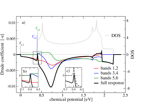
Figure 2: a) SGE Drude coefficient at $T=10$ K (black) and the intraband (red, blue, green) contribution. The DOS is shown in grey for comparison. b) Detail of the intraband contrinution around the Lifshitz point. c) Interband contribution (dashed) in the same region as b) arising from scattering between bands (3,4) and bands (5,6). Calculations have been done for a lattice with $6354\times 6354$ $k$ points.

Fig. 2 shows the Drude coefficient $D^{SGE}$ for the clean system and its decomposition into the contribution from the individual pair of bands as a function of chemical potential $\mu$. Close to the corresponding $\Gamma$ points (indicated by the vertical dashed lines) the individual contributions can be evaluated analytically and are given in the $6$th row of Tab. 1 and the $\mu$ dependence is implicit in the corresponding DOS $N_{0}(\mu)$. Up to $\mu\approx 0.4$ eV the full Drude response (black) is well described by the contribution of the lowest pair of bands (1,2) because the inter-band contributions arising from the mixing $(1,2)\leftrightarrow(3,4)$ and $(1,2)\leftrightarrow(5,6)$ are opposite in sign and almost compensate. The inter-band scattering $(3,4)\leftrightarrow(5,6)$ becomes significant upon crossing the Lifshitz point at $\mu\approx 0.4$ eV [cf. panel c)]. In this regime the small positive contributions from bands (3,4) and (5,6) [cf. 6th row of Tab. 1] are overcompensated by the negative $D^{SGE}$ from bands (1,2) together with a large negative inter-band contribution $(3,4)\leftrightarrow(5,6)$ which prevents the occurrence of a significant sign change in $D^{SGE}$ as a function of $\mu$. This sign change around the Lifshitz point is therefore very weak and confined to a very narrow chemical potential range (cf. panel b) of Fig. 2). Another sign change occurs in the high-filling regime around $\mu\approx 1.7$ eV.

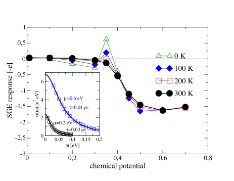
Figure 3: Regular part of the SGE response function as a function of chemical potential. Disorder potential is $V_{0}=0.1$ eV and calculations are performed on $24\times 24$ lattices.

The Drude SGE response is obtained in the clean limit which corresponds to a non-stationary situation when there is no dissipation and the momentum relaxation time $\tau$ becomes infinite. However, Fig. 2 suggests that the experimentally observed sign change in $\sigma^{SGE}$ around the Lifshitz point [15] may be supported by disorder which changes the relative contributions of intra- and inter-band processes to the SGE. We therefore proceed by evaluating the response for the disordered system by adding an impurity potential $V=\sum_{n}V_{n}{\bf 1}$ in the local basis of the $t_{2g}$ orbitals to the Hamiltonian Eq. (1). The $V_{n}$ are drawn from a flat distribution $-V_{0}\leq V_{n}\leq V_{0}$ and we average over typically $50$ impurity realizations and $100$ boundary conditions in order to minimize finite size effects. For a disorder potential $V=0.2$ eV the inset to Fig. 3 shows the optical conductivity for two values of the chemical potential below and above the Lifshitz point. By fitting with the Drude formula we find a transport scattering time $\tau\approx 0.3$ ps for $\mu=0.2$ eV and $\tau\approx 0.01$ ps for $\mu=0.6$ eV, which is of the same order of magnitude as that obtained with magnetotransport measurements on LAO/STO heterostructures [25]. The SGE response in the presence of disorder is shown in the main panel of Fig. 3. Compared to the clean case one observes a significant suppression in the regime where the chemical potential falls within the $d_{xy}$-bands. The sign change around the Lifshitz point is still confined to a narrow window, but is more pronounced than in the clean case. Finally, when the chemical potential enters the $d_{xz}\/d_{yz}$-bands we obtain a sizable SGE response and the overall behavior is in very good agreement with the gate voltage dependence of the spin galvanic effect as measured in Ref. [16] at $T=300$ K. In contrast, the voltage dependence of the SGE response in Ref. [15] has been measured at much lower temperature $T=7$ K and shows the sign change upon voltage reversal. At low temperature our results display two sign changes: from negative to positive $\sigma^{SGE}[-e]$ when $\mu$ is enters into bands (3,4) and back to negative $\sigma^{SGE}[-e]$ when $\mu$ moves inside bands (5,6). The latter we therefore associate with the experimentally observed sign change and one may expect a second sign reversal of the SGE when experimentally the gating could be tuned to larger negative values at low temperature, in agreement with our analytical analysis which in the diffusive limit yields a negative $\sigma^{SGE}[-e]$ close to the bottom of the xy-type bands (1,2) [cf. Tab. 1]. In this regard one may also speculate whether a more realistic implementation of disorder may help to extend the region of positive $\sigma^{SGE}[-e]$ deeper into the $d_{xy}$-band range (i.e. toward negative gate voltages). In fact, since $d_{xz}$- and $d_{yz}$-orbitals extend deeper into the STO bulk it is plausible to assume that they are less affected by disorder in the 2DEG system than the $d_{xy}$-states. This is also supported by the gate voltage dependence of the transport scattering time which shows a pronounced increase upon crossing the Lifshitz point [25] and a refinement of our computations in this regard opens a perspective for future investigations. Moreover, the Rashba SOC in STO-based heterostructures has been recently also analyzed within a ${\bf k}\cdot{\bf p}$ Luttinger-Kohn (LK) approach [26, 27] which provides an alternative to the asymmetry term $H_{I}$ in our hamiltonian. Differences occur in particular around the Lifshitz point where the LK model predicts a smaller Rashba SOC for the lowest pair of bands. Future studies should therefore be directed at clarifying the consequences of the LK model on the SGE and other transport response functions.

References

- Ivchenko and Pikus [1978] E. L. Ivchenko and G. E. Pikus, Soviet Journal of Experimental and Theoretical Physics Letters 27, 604 (1978).
- Vorob’ev et al. [1979] L. E. Vorob’ev, E. L. Ivchenko, G. E. Pikus, I. I. Farbshteǐn, V. A. Shalygin, and A. V. Shturbin, Soviet Journal of Experimental and Theoretical Physics Letters 29, 441 (1979).
- Ivchenko et al. [1989] E. L. Ivchenko, Y. B. Lyanda-Geller, and G. E. Pikus, JETP Lett. 50, 176 (1989).
- Edelstein [1990] V. M. Edelstein, Solid State Commun. 73, 233 (1990).
- Aronov and Lyanda-Geller [1989] A. G. Aronov and Y. B. Lyanda-Geller, JETP Lett. 50, 431 (1989).
- Bychkov and Rashba [1984] Y. A. Bychkov and E. I. Rashba, J. Phys. C 17, 6039 (1984).
- Ganichev et al. [2001] S. D. Ganichev, E. L. Ivchenko, S. N. Danilov, J. Eroms, W. Wegscheider, D. Weiss, and W. Prettl, Phys. Rev. Lett. 86, 4358 (2001).
- Ganichev et al. [2002] S. D. Ganichev, E. L. Ivchenko, V. V. Belkov, S. A. Tarasenko, M. Sollinger, D. Weiss, W. Wegscheider, and W. Prettl, Nature 417, 153 (2002).
- Ganichev et al. [2006] S. D. Ganichev, S. N. Danilov, P. Schneider, V. V. Bel’kov, L. E. Golub, W. Wegscheider, D. Weiss, and W. Prettl, Journal of Magnetism and Magnetic Materials 300, 127 (2006).
- Ganichev et al. [2016] S. D. Ganichev, M. Trushin, and J. Schliemann, “Handbook of spin transport and magnetism,” (Chapman and Hall, 2016) Chap. Spin polarisation by current.
- Sánchez et al. [2013] J. C. R. Sánchez, L. Vila, G. Desfonds, S. Gambarelli, J. P. Attané, J. M. D. Teresa, C. Magén, and A. Fert, Nature Commun. 4, 2944 (2013).
- Mellnik et al. [2014] A. R. Mellnik, J. S. Lee, A. Richardella, J. L. Grab, P. J. Mintun, M. H. Fischer, A. Vaezi, A. Manchon, E.-A. Kim, N. Samarth, and D. C. Ralph, Nature (London) 511, 449 (2014).
- Shiomi et al. [2014] Y. Shiomi, K. Nomura, Y. Kajiwara, K. Eto, M. Novak, K. Segawa, Y. Ando, and E. Saitoh, Physical Review Letters 113, 196601 (2014).
- Chauleau1 et al. [2016] J.-Y. Chauleau1, M. Boselli, S. Gariglio, R. Weil, G. de Loubens, J.-M. Triscone, and M. Viret, EPL 116, 17006 (2016).
- Lesne et al. [2016] E. Lesne, S. O. Yu Fu, J. C. Rojas-Sánchez, D. C. Vaz, H. Naganuma, G. Sicoli, J.-P. Attané, M. Jamet, E. Jacquet, J.-M. George, A. Barthélémy, H. Jaffrès, A. Fert, M. Bibes, and L. Vila, Nat. Mater. 15, 1261 (2016).
- Song et al. [2017] Q. Song, H. Zhang, T. Su, W. Yuan, Y. Chen, W. Xing, J. Shi, J. Sun, and W. Han, Science Advances 3, e1602312 (2017).
- Hwang et al. [2012] H. Y. Hwang, Y. Iwasa, M. Kawasaki, B. Keimer, N. Nagaosa, and Y. Tokura, Nature Materials 11, 103 (2012).
- Caprara [2016] S. Caprara, Nat. Mater. 15, 1224 (2016).
- Zhong et al. [2013] Z. Zhong, A. Tóth, and K. Held, Phys. Rev. B 87, 161102 (2013).
- Khalsa et al. [2013] G. Khalsa, B. Lee, and A. H. MacDonald, Phys. Rev. B 88, 041302 (2013).
- Kim et al. [2013] Y. Kim, R. M. Lutchyn, and C. Nayak, Phys. Rev. B 87, 245121 (2013).
- Shen et al. [2014] K. Shen, G. Vignale, and R. Raimondi, Phys. Rev. Lett. 112, 096601 (2014).
- [23] Note that for the splitting we take a value between the theoretical ( eV) end the experimental one ( eV). As long as and this has no influence on our further results.
- Zhou et al. [2015] J. Zhou, W.-Y. Shan, and D. Xiao, Phys. Rev. B 91, 241302(R) (2015).
- Liang et al. [2015] H. Liang, L. Cheng, L. Wei, Z. Luo, G. Yu, C. Zeng, and Z. Zhang, Phys. Rev. B 92, 075309 (2015).
- van Heeringen et al. [2013] L. W. van Heeringen, G. A. de Wijs, A. McCollam, J. C. Maan, and A. Fasolino, Phys. Rev. B 88, 205140 (2013).
- van Heeringen et al. [2017] L. W. van Heeringen, A. McCollam, G. A. de Wijs, and A. Fasolino, Phys. Rev. B 95, 155134 (2017).