Radiative corrections to the average bremsstrahlung energy loss of high-energy muons

Abstract

High-energy muons can travel large thicknesses of matter. For underground neutrino and cosmic ray detectors the energy loss of muons has to be known accurately for simulations. In this article the next-to-leading order correction to the average energy loss of muons through bremsstrahlung is calculated using a modified Weizsäcker-Williams method. An analytical parametrisation of the numerical results is given.

1 Introduction

The muon bremsstrahlung cross section has been studied extensively for many years [1, 2, 3, 4, 5]. Together with the production of electron-positron pairs [6, 7, 8, 9] and the inelastic nuclear interaction [10, 11, 12] it describes the dominant contribution to the energy loss of high-energy muons.

Muons with energies of tens to hundreds of TeV can travel distances of the order of several kilometers. Therefore it is necessary to know the average energy loss per unit length

$$-\left\langle\frac{\,\mathrm{d}E}{\,\mathrm{d}x}\right\rangle=N\int Ev\frac{\,\mathrm{d}\sigma}{\,\mathrm{d}v}\,\mathrm{d}v$$ (1)

accurately. Here $v=(E-E^{\prime})/E$ is the relative energy loss per interaction, and $N$ is the number density of target atoms. Previous calculations took into account the modification of the Coulomb interaction with the nucleus by elastic and inelastic nuclear form factors, the contribution of atomic electrons as target for muon bremsstrahlung and the inelastic interaction with the target nucleus. This article discusses the correction of the energy loss through virtual and real radiative corrections. Since this correction is small compared to the main contribution, we restrict our treatment of the nucleus to elastic atomic and nuclear form factors.

The energy loss is of importance for underground detectors for two reasons: on the one hand, the energy loss is needed to predict the spectrum of muons that will reach the detector; on the other hand the energy lost by a muon inside the detector on a given length is used to reconstruct the energy of the radiating particle. The energy reconstruction is further complicated by its sensitivity to the distribution of energy losses and their correlation to the energy of the muon. Especially rare large stochastic energy losses enlarge the variance of the energy loss per unit length. As a first step to revisit this problem, in the present article, the muon energy dependent average energy loss per length is calculated.

In the calculation of radiative corrections in QED processes with virtual photons give rise to logarithmically divergent integrals; to obtain a finite result, it is necessary to add the cross section for the emission of an additional photon with energy $\omega<\omega_{\text{min}}$ which cancels this divergence. Usually $\omega_{\text{min}}$ is identified with the finite energy resolution of the detector and assumed to be small compared to the mass of the radiating particle, such that the approximation of classical currents can be used. The contribution of harder photons indistinguishable from a single photon is then evaluated numerically according to the conditions of the experiment (see e. g. [13]). In the problem of muon propagation, however, the particle may traverse several kilometers of material before the energy losses can be seen by the detector. Therefore the cross section has to be integrated over all kinematically allowed states of the additional photon. So the energy loss depends only on the primary energy of the muon.

Unless stated otherwise, all equations are presented in a system of units where $\hbar=c=m_{\mu}=1$.

2 Method

The calculation reported here is based on the Weizsäcker-Williams method [14, 15], which approximates the effect of a nucleus by a spectrum of equivalent photons. This method allows to express the bremsstrahlung cross section through the Compton cross section convolved with the equivalent photon flux. Using the radiative corrections to the Compton effect in [16], the radiative corrections to the bremsstrahlung spectrum were first calculated in the soft-photon approximation in [17] for an unscreened or totally screened nucleus.

2.1 Conventional Weizsäcker-Williams method

Considering the collision of a fast muon with an atom, we introduce two systems of reference: the laboratory system $K_{Z}$ in which the atom is at rest and the muon has a Lorentz factor $\gamma\gg 1$, and the system $K_{\mu}$ in which the muon is at rest and the atom has a Lorentz factor of $\gamma$. The interaction of the muon with the atom can be described symbolically by the diagram in Fig. 1$(a)$. The shaded blob denotes the internal part of the diagram, the double line $X$ denotes particles created in the collision.

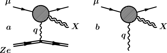
Figure 1: $(a)$ Symbolic Diagram of interaction of a muon with an atom. $(b)$ Equivalent Diagram in the Weizsäcker-Williams method. The shaded blob denotes the internal part of the diagram. $X$ denotes particles created in the collision.

Diagram Fig. 1$(b)$ describes a similar process due to collision of a real photon with a muon. We consider two cases here:

1. $X=\gamma$. In this case $(a)$ is bremsstrahlung and we assume that the blob also contains radiative corrections; $(b)$ is Compton scattering with radiative corrections.

2. $X=2\gamma$. In this case $(a)$ is double bremsstrahlung and $(b)$ is double Compton scattering.

In the Weizsäcker-Williams method the field of the atom in $K_{\mu}$ is replaced by a flux of equivalent photons with the spectrum $n(\omega)\,\mathrm{d}\omega$. This allows to relate the differential cross sections of the processes $(a)$ and $(b)$ by the relation

$$\,\mathrm{d}\sigma_{a}=\,\mathrm{d}\sigma_{b}n(\omega)\,\mathrm{d}\omega,$$ (2)

and for the total cross section

$$\int\,\mathrm{d}\sigma_{a}=\int\,\mathrm{d}\sigma_{b}n(\omega)\,\mathrm{d}\omega.$$ (3)

It is convenient to calculate the cross section $\sigma_{b}$ in the frame $K_{\mu}$. Since the cross section is Lorentz-invariant, the transition from $K_{\mu}$ to $K_{Z}$ is trivial.

In $K_{Z}$ the average energy loss per unit length caused by the process $(a)$ is given by

$$-\left\langle\frac{\,\mathrm{d}E}{\,\mathrm{d}x}\right\rangle=NE\Sigma,\quad\Sigma=\frac{1}{E}\int(E-E^{\prime})\,\mathrm{d}\sigma_{a}.$$ (4)

where $E$ ($E^{\prime}$) is the initial (final) muon energy, $N$ is the number density of target atoms per unit volume. The quantity $\Sigma$ can be rewritten in a relativistically invariant form as

$$\Sigma=\frac{1}{(up)}\int((up)-(up^{\prime}))\,\mathrm{d}\sigma_{a},$$ (5)

where $u$ is the 4-velocity of the atom and $p,p^{\prime}$ are the initial and final 4-momenta of the muon respectively, $(up)=u^{0}p^{0}-\mathbf{up}$ is the scalar product of 4-vectors. Using (2) it is possible to rewrite this as

$$\Sigma=\int\frac{(up)-(up^{\prime})}{(up)}\,\mathrm{d}\sigma_{b}n(\omega)\,\mathrm{d}\omega.$$ (6)

In this equation we will calculate the integrand in the $K_{\mu}$ frame. For Compton scattering the energy-momentum conservation gives $(u,p-p^{\prime})=(u,q^{\prime}-q)$, where $q$ ($q^{\prime}$) is the initial (final) photon 4-momentum. In the frame $K_{\mu}$ we have $(uq)/\gamma=\omega(1-\beta)\approx\omega/(2\gamma^{2})$, where $\omega$ is the initial photon energy. Since $\omega\sim\gamma$, the ratio $(uq)/\gamma\sim 1/\gamma$ is negligible. The other term is

$$\frac{(uq^{\prime})}{\gamma}=\omega^{\prime}(1-\beta\cos\theta)\approx\frac{1}{2}\omega^{\prime}(\theta^{2}+1/\gamma^{2}).$$ (7)

In Compton scattering $\theta\lesssim 1/\sqrt{\gamma}$ [18] and the second term in parentheses is negligible. Therefore we obtain for the first case

$$1-\frac{(up^{\prime})}{(up)}\approx 1-\frac{\omega^{\prime}}{\omega}.$$ (8)

Similarly for double Compton scattering we have

$$1-\frac{(up^{\prime})}{(up)}\approx\omega_{1}(1-\cos\theta_{1})+\omega_{2}(1-\cos\theta_{2}),$$ (9)

where $\omega_{1,2},\theta_{1,2}$ are the energies and angles of the final photons.

2.2 Modified Weizsäcker-Williams method

For a point-like nucleus, the pseudophoton flux in the rest frame of the muon is given by [18]

$$n(\omega)\,\mathrm{d}\omega=\frac{2}{\pi}Z^{2}\alpha\frac{\,\mathrm{d}\omega}{\omega}\ln\frac{\gamma}{\omega}$$ (10)

where $\gamma$ is the Lorentz factor of the incident particle in the laboratory frame, or, equivalently the Lorentz factor of the nucleus in the rest frame of the muon.

For muons, it is necessary to take into account the extended nucleus and the screening of the nucleus by atomic electrons, because the characteristic momentum transfer of $q\sim m_{\mu}$ is comparable to the inverse radius of the nucleus and the minimum momentum transfer $\delta\sim m_{\mu}^{2}/E$ is comparable to or smaller than the inverse radius of the atom [3].

For an atom with nuclear and atomic formfactors $F_{\text{n}}(q^{2}),F_{\text{a}}(q^{2})$ we obtain

$$n(\omega)\,\mathrm{d}\omega=\frac{\alpha Z^{2}\,\mathrm{d}\omega}{\pi\omega}\int\limits_{\omega^{2}/\gamma^{2}}^{\infty}\frac{\tau-\omega^{2}/\gamma^{2}}{\tau^{2}}\,\left(F_{\text{n}}(\tau)-F_{\text{a}}(\tau)\right)^{2}\,\mathrm{d}\tau.$$ (11)

In this work the charge distribution of the nucleus and of the atomic electrons are described by a Gaussian and an exponential distribution, respectively, resulting in the form factors

$$F_{\text{n}}(q^{2}) =\exp\left[-\frac{q^{2}R_{\text{n}}^{2}}{6}\right],$$ (12)

$$F_{\text{a}}(q^{2}) =\left[1+\frac{q^{2}R_{\text{a}}^{2}}{12}\right]^{-2}$$ (13)

with $R$ the Rms-radius of the charge distribution. The atomic and nuclear radius can be parametrised for light and medium nuclei as [19]

$$R_{\text{n}} =1.27A^{0.27}$\mathrm{f}\mathrm{m}$,$$ (14)

$$R_{\text{a}} =\frac{183Z^{-1/3}}{2.718m_{\text{e}}}$$ (15)

with $$Z A$$ the nucleus charge and its mass number, and for hydrogen

$$R_{\text{p}} =$0.85\text{\,}\mathrm{f}\mathrm{m}$.$$ (16)

With the above formfactors, the calculation of the pseudophoton flux integral gives

$$n(\omega)\,\mathrm{d}\omega=\frac{\alpha Z^{2}}{\pi}\left[\frac{1}{(bz+1)^{2}}\left(-\frac{17}{6}-4b^{2}z^{2}-7bz\right)\right.$$

$$-2\exp\left(\frac{a}{b}\right)(az-2bz+a/b-1)\operatorname{Ei}(1,a(z+1/b))$$ (17)

$$-(2az+4bz+2)\operatorname{Ei}(1,az)+(2az+1)\operatorname{Ei}(1,2az)$$

$$\left.\phantom{\frac{1}{1}}+(4bz+1)\ln\left(1+\frac{1}{bz}\right)-\mathrm{e}^{-2az}+4\mathrm{e}^{-az}\right]\frac{\,\mathrm{d}\omega}{\omega},$$

where $\operatorname{Ei}(1,x)=\int_{x}^{\infty}e^{-t}/t\,\mathrm{d}t$ is the exponential integral, $z=\omega^{2}/\gamma^{2}$, $a=R_{\text{n}}^{2}/6$, $b=R_{\text{a}}^{2}/12$.

2.3 Corrections to energy loss

The contribution to the energy loss of a pseudophoton with energy $\omega$ in the rest system of the charged projectile can be conveniently expressed by the angles and energies of the final particles in this system as

$$\gamma\int\left(1-\frac{\omega^{\prime}}{\omega}\right)d\sigma(\omega,\omega^{\prime})$$ (18)

for virtual radiative corrections, where $d\sigma(\omega,\omega^{\prime})$ is the differential cross section for Compton scattering and the scattering angle $\theta$ is determined by conservation laws; and

$$\gamma\int[\omega_{1}(1-\cos\theta_{1})+\omega_{2}(1-\cos\theta_{2})]d\sigma(\omega,\omega_{1},\omega_{2},\theta_{1},\theta_{2})$$ (19)

for the double bremsstrahlung contribution, where $d\sigma(\omega,\omega_{1},\omega_{2},\theta_{1},\theta_{2})$ is the differential cross section for double Compton scattering, dependent on the initial and final photon energies $\omega$ and $\omega_{1},\omega_{2}$ and the scattering angles $\theta_{1},\theta_{2}$; the azimuthal angle between the two photons is determined by conservation laws. All quantities refer to the rest system of the muon. This formulation improves the numerical stability compared to using the angles in the lab frame, because the cross section is strongly peaked in the forward direction, while this peak is much broader in the rest frame.

In addition, the contribution from vacuum polarization was calculated directly. The loop correction to the virtual photon coupled to the atom can be interpreted as a factor modifying the form factor of the atom.

3 Results

Let us represent Eq. (30) from [16] in the form

$$P=P_{0}+P_{1}\ln\lambda$$ (20)

where $\lambda$ is the fictitious photon mass necessary to regularize the infrared divergences which cancels out in the final result. The functions $P_{0}$ and $P_{1}$ depend only on the initial and final photon energies $\omega,\omega^{\prime}$. Then the virtual radiative corrections to the differential Compton cross section are given by

$$\,\mathrm{d}\sigma_{\text{corr}}=-\alpha r_{\mu}^{2}(P_{0}+P_{1}\ln\lambda)\frac{\,\mathrm{d}\omega}{\omega^{2}}$$ (21)

and we obtain

$$\sigma_{\text{corr}}=-\frac{\alpha r_{\mu}^{2}}{\omega^{2}}\int\limits_{\omega_{*}}^{\omega}(P_{0}+P_{1}\ln\lambda)\,\mathrm{d}\omega^{\prime}$$ (22)

for the total cross section, where $\omega_{*}=\omega/(1+2\omega)$. To determine the correction to the average energy loss we have to calculate the integral

$$-\frac{1}{\omega^{2}}\int\limits_{\omega_{*}}^{\omega}(P_{0}+P_{1}\ln\lambda)\left(1-\frac{\omega^{\prime}}{\omega}\right)\,\mathrm{d}\omega^{\prime}.$$ (23)

The results can be expressed through the following functions:

$$A_{i} =-\frac{1}{\omega^{2}}\int\limits_{\omega_{*}}^{\omega}P_{i}\,\mathrm{d}\omega^{\prime}$$ (24)

$$B_{i} =-\frac{1}{\omega^{2}}\int\limits_{\omega_{*}}^{\omega}P_{i}\left(1-\frac{\omega^{\prime}}{\omega}\right)\,\mathrm{d}\omega^{\prime},$$ (25)

$$i =1,2.$$

The graphs of the functions $A_{0,1},B_{0,1}$ which only depend on $\omega$ are shown in Fig. 2.

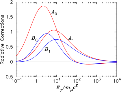
Figure 2: Numerical results of the integration over angles and energies for the contribution of the pseudophoton with energy $E_{\gamma}$ for the functions defined in (24), (25).

For the calculation of the integral (9) we used the cross section from [20]. The integral diverges as $\omega_{1,2}\rightarrow 0$, so we integrated over the region $\omega_{1,2}>\omega_{\text{min}}$. Let us denote the result of this integration as $\alpha r_{\mu}^{2}\gamma X(\omega,\omega_{\text{min}})$. The sum

$$f(\omega)\equiv X(\omega,\omega_{\text{min}})+B_{0}(\omega)+B_{1}(\omega)\ln(2\omega_{\text{min}})$$ (26)

in the limit $\omega_{\text{min}}\rightarrow 0$ does not depend on $\omega_{\text{min}}$. Numerical calculations for $\omega_{\text{min}}=10^{-4}$ and $\omega_{\text{min}}=10^{-5}$ give practically the same result (here we use the known relation $\lambda=2\omega_{\text{min}}$). For the convenience of further calculations we have obtained the following approximate formula:

$$f(\omega)=405\omega\left[1-\frac{(0.006\omega)^{2}}{16+(0.006\omega)^{4}}\right]\frac{\ln(1+0.00654\omega)}{1+4\ln^{2}(\omega+1)+\omega^{2}},$$ (27)

The comparison between the numerical results and this approximation is shown in Fig. 3.

Figure 3: Comparison of the numerical results (solid line) and the analytical parametrisation (27) (dots).

By numerical integration over the product of the pseudophoton flux and this function the energy loss is obtained. It can be parametrized by the function

$$-\frac{1}{E}\left\langle\frac{\,\mathrm{d}E}{\,\mathrm{d}x}\right\rangle=Z^{2}\alpha^{2}Nr_{\mu}^{2}c_{1}\ln\frac{R_{\text{a}}/(R_{\text{n}}c_{2})}{1+R_{\text{a}}/(R_{\text{n}}c_{2})\cdot c_{3}/\gamma}$$ (28)

with

$$c_{1} =$8.303$,$$ (29)

$$c_{2} =$0.999$,$$ (30)

$$c_{3} =$4.099$+$6.335$Z^{1/3}.$$ (31)

The additional contribution of vacuum polarization can be parametrized as

$$-\frac{1}{E}\left\langle\frac{\,\mathrm{d}E}{\,\mathrm{d}x}\right\rangle=Z^{2}\alpha^{2}Nr_{\mu}^{2}3\ln\frac{Y}{1+\xi Y/(\gamma R_{\text{N}})}$$ (32)

with

$$Y =\frac{R_{\text{a}}}{16.7R_{\text{N}}},$$ (33)

$$\xi =0.1+0.0921A^{0.8}.$$ (34)

3.1 Ratio to the main contribution

When the main contribution to the bremsstrahlung energy loss is calculated in the modified Weizsäcker-Williams method with the above form factors, the ratio between the radiative correction and the main contribution is independent of $Z$ and $A$ and can be parametrized as

$$-\frac{1}{E}\left\langle\frac{\,\mathrm{d}E}{\,\mathrm{d}x}\right\rangle_{\text{rad}}=-\frac{1}{E}\left\langle\frac{\,\mathrm{d}E}{\,\mathrm{d}x}\right\rangle_{0}\alpha\delta(\gamma)$$ (35)

with

$$\delta(\gamma)=2.66\frac{\xi-1}{\xi+1},\quad\xi=$0.0406$\sqrt{\gamma}+3.39$$ (36)

for light and medium nuclei and

$$\delta(\gamma)=2.77\frac{\xi-1}{\xi+1},\quad\xi=0.02\sqrt{\gamma}+5.32.$$ (37)

for hydrogen.

4 Conclusion

The radiative corrections to the average energy loss of muons by bremsstrahlung have been calculated using a modified Weizsäcker-Williams method. It was found that the energy loss is increased by about $2\text{\,}\%$ in the complete screening regime. An analytical parametrization of the numerical results has been obtained.

To estimate the accuracy of the calculation the contribution of leading order bremsstrahlung was calculated using an exact calculation and the Weizsäcker-Williams method with the used formfactors. The difference between the exact numerical results and the result by the Weizsäcker-Williams method is approximately $1\text{\,}\%$ (cf. Fig. 4).

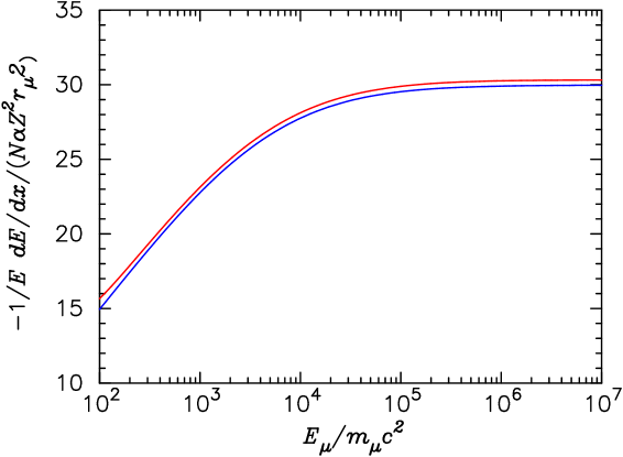
Figure 4: Energy losses in oxygen due to bremstrahlung. The red line shows the calculation using the Weizsäcker-Williams method with the photon spectrum (17), the blue line is the usual calculation with the formfactors (12), (13). The difference between the curves is approximately $1\text{\,}\%$.

This result is important for underground muon and neutrino detectors, because it is a step to reduce the uncertainty on the energy loss of muons on their passage to the detector.

References

References

- [1] A. A. Petrukhin, V. V. Shestakov, The influence of nuclear and atomic form factors on the muon bremsstrahlung cross section, Canad. J. Phys. 46 (1968) S377.
- [2] Y. M. Andreev, L. B. Bezrukov, E. V. Bugaev, Excitation of a target in muon bremsstrahlung, Phys. At. Nucl. 57 (1994) 2066–2074.
- [3] Y. M. Andreev, E. V. Bugaev, Muon bremsstrahlung on heavy atoms, Phys. Rev. D 55 (1997) 1233–1243.
- [4] S. R. Kelner, R. P. Kokoulin, A. A. Petrukhin, About cross section for high-energy muon bremsstrahlung, Preprint MEPhI 024-95, Moscow (1995).
- [5] S. R. Kelner, R. P. Kokoulin, A. A. Petrukhin, Bremsstrahlung from muons scattered by atomic electrons, Phys. At. Nucl. 60 (1997) 576–583.
- [6] S. R. Kelner, Y. D. Kotov, Muon energy loss to pair production, Sov. J. Nucl. Phys. 7 (1968) 237–240.
- [7] R. P. Kokoulin, A. A. Petrukhin, Analysis of the cross section of direct pair production by fast muons, in: Proc. 11th Int. Conf. on Cosmic Rays, Budapest 1969, Vol. 29, Suppl. 4, Acta Phys. Acad. Sci. Hung., 1970, pp. 277–284.
- [8] R. P. Kokoulin, A. A. Petrukhin, Influence of the nuclear formfactor on the cross section of electron pair production by high-energy muons, in: Proc. 12th Int. Conf. on Cosmic Rays, Hobart 1971, Vol. 6, 1971, pp. 2436–2444.
- [9] S. R. Kelner, Pair production in collisions between muons and atomic electrons, Phys. At. Nucl. 61 (1998) 448–456.
- [10] H. Abramowicz, E. M. Levin, A. Levy, U. Maor, A parametrization of above the resonance region for , Phys. Lett. B 269 (1991) 465–476. doi:doi:10.1016/0370-2693(91)90202-2.
- [11] H. Abramowicz, A. Levy, The ALLM parametrization of : an update, arXiv:hep-ph/9712415 (1997).
- [12] E. V. Bugaev, Y. V. Shlepin, Photonuclear interaction of high energy muons and tau leptons, Nucl. Phys. B Proc. Suppl. 122 (2003) 341–344. doi:10.1016/S0920-5632(03)80414-0.
- [13] A. B. Arbuzov, Radiative corrections to high energy muon bremsstrahlung on heavy nuclei, JHEP 01 (2008) 031.
- [14] C. F. v. Weizsäcker, Ausstrahlung bei Stößen sehr schneller Elektronen, Z. Physik 88 (1934) 612–625. doi:10.1007/BF01333110.
- [15] E. J. Williams, Nature of the high energy particles of penetrating radiation and status of ionization and radiation formulae, Phys. Rev. 45 (1934) 729–730. doi:10.1103/PhysRev.45.729.
- [16] L. M. Brown, R. P. Feynman, Radiative corrections to Compton scattering, Phys. Rev. 85 (1952) 231.
- [17] K. Mork, H. Olsen, Radiative corrections. I. High-energy bremsstrahlung and pair production, Phys. Rev. 140 (1965) B 1661.
- [18] V. B. Berestetsky, E. M. Lifshitz, L. P. Pitaevsky, Kvantovaya elektrodinamika (Quantum Electrodynamics), Nauka, Moscow, 1980.
- [19] A. V. Butkevich, R. P. Kokoulin, G. V. Matushko, S. P. Mikheyev, Comments on multiple scattering of high-energy muons in thick layers, Nucl. Instr. Meth. in Phys. Res. A 488 (2002) 282.
- [20] F. Mandl, T. H. R. Skyrme, Theory of the double Compton effect, Proc. Roy. Soc. Lond. A Math. Phys. Sci. 215 (1952) 497.