Theory of Dzyaloshinskii domain wall tilt in ferromagnetic nanostrips

Abstract

We present an analytical theory of domain wall tilt due to a transverse in-plane magnetic field in a ferromagnetic nanostrip with out-of-plane anisotropy and Dzyaloshinskii-Moriya interaction (DMI). The theory treats the domain walls as one-dimensional objects with orientation-dependent energy, which interact with the sample edges. We show that under an applied field the domain wall remains straight, but tilts at an angle to the direction of the magnetic field that is proportional to the field strength for moderate fields and sufficiently strong DMI. Furthermore, we obtain a nonlinear dependence of the tilt angle on the applied field at weaker DMI. Our analytical results are corroborated by micromagnetic simulations.

I Introduction

Domain wall (DW) statics and dynamics in thin-film ferromagnetic systems have been a subject of intense experimentalAtkinson et al. (2003); Yamaguchi et al. (2004); Par ; Hoffmann and Bader (2015) and theoretical Tatara and Kohno (2004); Thiaville et al. (2005); Tretiakov et al. (2008); Khvalkovskiy et al. (2013); Shibata et al. (2011) studies over the last decades due to their direct relevance to spintronic memoryParkin et al. (2008) and logic devices. Allwood et al. (2005) Recently, it has been realized that ferromagnets with Dzyaloshinskii-Moriya interactionDzyaloshinsky (1958); Moriya (1960) (DMI) may offer more benefits in this direction, Tretiakov and Ar. Abanov (2010); Thiaville et al. (2012); Boulle et al. (2013) which led to an enormous experimental progress for these systems. Emori et al. (2014); Franken et al. (2014); Benitez et al. (2015); Boulle et al. (2016); Yu et al. (2016)

Due to their better technological suitability as smaller and more robust carriers of information in spintronic nanodevices, the DWs in ultrathin ferromagnetic films with out-of-plane anisotropy and interfacial DMI have now become the primary objects of experimental interest. Emori et al. (2014); Franken et al. (2014); Benitez et al. (2015); Boulle et al. (2016); Yu et al. (2016) Moreover, it was discovered that the DWs move much more efficiently in these systems due to spin-orbit torques.Garello et al. (2013); Khvalkovskiy et al. (2013); Ado et al. (2017) It was also demonstrated that in these systems the DW equilibrium structure changes from Bloch to Néel type in the presence of strong DMI. Chen et al. (2013) Following a theoretical study,Thiaville et al. (2012) we refer below to this new type of magnetic DWs as Dzyaloshinskii domain walls.

Boulle et al.Boulle et al. (2013) were the first to discover numerically that these DWs develop a tilt under in-plane magnetic fields and applied currents. This DW tilt was shown to depend on the DMI and field strengths. It was followed by several more attempts to investigate this phenomena theoreticallyMartinez et al. (2014); Vandermeulen et al. (2016) and multiple experimental studies.Emori et al. (2014); Franken et al. (2014); Yu et al. (2016) However, up to now there is still lack of a unifying theory of the DW tilt and its dependence on the in-plane magnetic field.

In this paper, we explain these important findings on more solid theoretical grounds, using variational analysis of the magnetic energy functional. We study a DW in a thin nanostrip with perpendicular magnetic anisotropy (PMA) and interfacial DMI in the presence of a magnetic field applied in the plane of the strip and perpendicular to its axis, see Fig. 1 for an example. For this system we analytically develop a proper reduced geometric variational model built on exact one-dimensional (1D) DW solutions to describe the equilibrium tilted two-dimensional (2D) DW configurations. These exact 1D magnetization profiles are in general neither Néel nor Bloch type, but can be easily computed numerically for all relevant values of the parameters. We also derive explicit analytical expressions by expanding the DW energy in the applied field or DMI strengths.

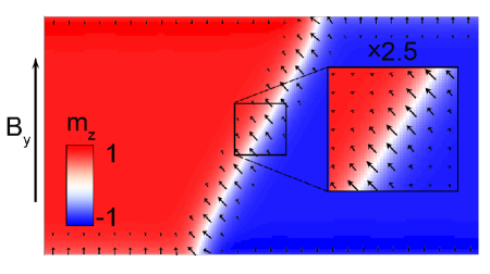
Figure 1: An example of a tilted domain wall in a transverse in-plane magnetic field computed using micromagnetic simulations. The material parameters are: $A=10^{-11}$J/m, $K=1.25\times 10^{6}$ J/m³, $M_{s}=1.09\times 10^{6}$ A/m, $D=2.4$ mJ/m² and $B_{y}=\mu_{0}H=80$ mT (see Sec. II for precise definitions).

In the reduced 2D variational problem, we treat the DW as a curve whose shape is determined by minimizing an appropriate geometric energy functional. As a result we show that the DW in equilibrium remains straight despite the fact that the wall energy is a function of its local orientation. In particular, for small fields the tilt angle is found to be proportional to the transverse magnetic field strength. One of the features of our 2D analysis is the necessity to include the edge DWs found earlier in the context of skyrmions.Rohart and Thiaville (2013) These edge DWs can be seen in Fig. 1 along the upper and lower strip edges. We show that the contribution of the edge DWs is also essential for determining the proper tilt angle. This is because the total DW energy contains contributions from both the internal and the edge DWs, and it is the competition among them that determines the tilt angle. We find that the effect of the edge DWs becomes weaker when the DMI strength is reduced, whereas the internal DW energy has a nontrivial dependence on the DMI, magnetic field, and wall orientation that have to be properly accounted to determine the equilibrium tilt angle.

The main advantage of our reduced geometric variational model for tilted DWs is its considerable simplicity compared to the full micromagnetic description. Specifically, it allows for a detailed analytical treatment, which highlights the key physical features of tilted DWs mediated by interfacial DMI in PMA nanostructures. In particular, it yields explicit closed-form expressions for the dependence of the equilibrium tilt angle for a wide range of the material parameters and applied fields. The obtained analytical predictions are found to be in excellent agreement with the results of micromagnetic simulations, indicating that the reduced model captures all the essential physical aspects of the considered system.

The paper is organized as follows. In Sec. II we introduce the full micromagnetic model and its 2D reduction appropriate for infinite ultrathin ferromagnetic nanostrips. In Sec. III the theory of edge domain walls is presented, and in Sec. IV a detailed analysis of 1D interior wall profiles is carried out. Next, in Sec. V we demonstrate how the theory of 1D domain walls developed in the preceding sections is applied to a Dzyaloshinskii DW in an infinite 2D nanostrip. In Sec. VI we compare our analytical theory with micromagnetic simulations and show a good agreement between them. Here the additional effect of dipolar interactions is also discussed. Finally, a summary and some concluding remarks are presented in Sec. VII.

II Model

We consider a thin ferromagnetic nanostrip exhibiting PMA and interfacial DMI under the influence of an in-plane magnetic field. We start with a three-dimensional micromagnetic energy Hubert and Schäfer (1998); Bogdanov and Yablonskii (1989); Fert (1990); Bogdanov and Hubert (1994) (in the SI units):

$$E(\mathbf{M}) =\int_{\Omega}\left({A\over M_{s}^{2}}|\nabla\mathbf{M}|^{2}+{K\over M_{s}^{2}}|\mathbf{M}_{\perp}|^{2}-\mu_{0}\mathbf{M}\cdot\mathbf{H}\right)d^{3}r$$

$$+\mu_{0}\int_{\mathbb{R}^{3}}\int_{\mathbb{R}^{3}}{\nabla\cdot\mathbf{M}(\mathbf{r})\,\nabla\cdot\mathbf{M}(\mathbf{r}^{\prime})\over 8\pi|\mathbf{r}-\mathbf{r}^{\prime}|}\,d^{3}r\,d^{3}r^{\prime}$$

$$+{Dd\over M_{s}^{2}}\int_{\partial\Omega_{0}}\Big{(}\overline{M}_{\parallel}\nabla\cdot\overline{\mathbf{M}}_{\perp}-\overline{\mathbf{M}}_{\perp}\cdot\nabla\overline{M}_{\parallel}\Big{)}d^{2}r.$$ (1)

Here $\mathbf{M}=\mathbf{M}(\mathbf{r})$ is the magnetization vector at point $\mathbf{r}=(x,y,z)\in\Omega\subset\mathbb{R}^{3}$, where $\Omega=(-L/2,L/2)\times(-W/2,W/2)\times(0,d)$ is the nanostrip of length $L$, width $W$ and thickness $d$, and $\mathbf{M}_{\perp}$ and $M_{\parallel}$ are the in-plane and out-of-plane components of $\mathbf{M}$, respectively. The terms in Eq. (II) are, respectively: the exchange, uniaxial perpendicular anisotropy, Zeeman, magnetostatic interactions and the interfacial DMI terms, and $M_{s}=|\mathbf{M}|$, $A$, $K$, $\mathbf{H}$ and $D$ are the saturation magnetization, exchange stiffness, anisotropy constant, applied magnetic field and the DMI strength. As usual, $\mu_{0}$ is the permeability of vacuum. In the magnetostatic energy term, the vector field $\mathbf{M}(\mathbf{r})$ is extended by zero outside $\Omega$, and $\nabla\cdot\mathbf{M}$ is understood distributionally (i.e., it includes the contributions of boundary charges). Since the considered DMI is due to interfacial effects, its contribution to the energy is via a surface integral over the bottom film surface $\partial\Omega_{0}$ corresponding to an interface between the ferromagnet and a heavy metal, and $\overline{\mathbf{M}}=(\overline{\mathbf{M}}_{\perp},\overline{M}_{\parallel})$ is the value of $\mathbf{M}$ on $\partial\Omega_{0}$. However, using the standard convention, we normalize the DMI strength parameter $D$ to a unit volume of the ferromagnet.

We assume that the applied magnetic field is in the plane of the film and is normal to the strip axis, i.e., $\mathbf{H}=H\hat{\mathbf{y}}$, where $\hat{\mathbf{y}}$ is the unit vector in the direction of the $y$-axis. We also consider films which are much thinner than the exchange length $\ell_{ex}=\sqrt{2A/(\mu_{0}M_{s}^{2})}$, so that the magnetization in $\Omega$ is constant along the film thickness. Measuring lengths in the units of $\ell_{ex}$ and setting $\mathbf{M}(x,y,z)=M_{s}\mathbf{m}(x,y)$ with $|\mathbf{m}|=1$ in $\Omega$, we can rewrite the energy, to the leading orderGioia and James (1997) in $d/\ell_{ex}$, in the units of $Ad$ as

$$E(\mathbf{m}) \simeq\int_{-l/2}^{l/2}\int_{-w/2}^{w/2}\Big{[}|\nabla\mathbf{m}|^{2}+(Q-1)|\mathbf{m}_{\perp}|^{2}-2h\hat{\mathbf{y}}\cdot\mathbf{m}_{\perp}$$

$$\quad+\kappa\left(m_{\parallel}\nabla\cdot\mathbf{m}_{\perp}-\mathbf{m}_{\perp}\cdot\nabla m_{\parallel}\right)\Big{]}\,dy\,dx.$$ (2)

Here we defined $\mathbf{m}_{\perp}\in\mathbb{R}^{2}$ and $m_{\parallel}\in\mathbb{R}$ to be the respective in-plane and out-of-plane components of the unit magnetization vector $\mathbf{m}$, introduced the dimensionless parameters

$$Q={2K\over\mu_{0}M_{s}^{2}},\quad\kappa=D\sqrt{2\over\mu_{0}M_{s}^{2}A},\quad h={H\over M_{s}},$$ (3)

and defined the rescaled nanostrip dimensions $l=L/\ell_{ex}$ and $w=W/\ell_{ex}$. In Eq. (3), $Q>1$ is the material’s quality factor yielding PMA, $\kappa$ is the dimensionless DMI strength, which without loss of generality, may be assumed positive, and $h$ is the dimensionless applied field strength.

We are interested in the case of long nanostrips corresponding to $l\gg w$. Note that when $l\to\infty$, the energy in Eq. (II) diverges even if $h=0$ because of the presence of edge domain walls giving $O(l)$ contribution to the energy.Rohart and Thiaville (2013); Muratov and Slastikov (2016) Therefore, in order to pass to the limit $l\to\infty$ we need to subtract from $E$ the contribution of the one-dimensional ground state energy $e_{0}(h,w)=\min E_{0}(\mathbf{m})$, where

$$E_{0}(\mathbf{m}) =\int_{-w/2}^{w/2}\Big{[}|\mathbf{m}^{\prime}|^{2}+(Q-1)|\mathbf{m}_{\perp}|^{2}-2h\hat{\mathbf{y}}\cdot\mathbf{m}_{\perp}$$

$$\quad+\kappa\left((\hat{\mathbf{y}}\cdot\mathbf{m}_{\perp}^{\prime})m_{\parallel}-(\hat{\mathbf{y}}\cdot\mathbf{m}_{\perp})m_{\parallel}^{\prime}\right)\Big{]}\,dy.$$ (4)

The precise functional form of $e_{0}(h,w)$ is the subject of Sec. III.

Putting everything together, we now write the expression for the energy that describes a Dzyaloshinskii domain wall running across the nanostrip as

$$E(\mathbf{m}) =\int_{-\infty}^{\infty}\int_{-w/2}^{w/2}\Big{[}|\nabla\mathbf{m}|^{2}+(Q-1)|\mathbf{m}_{\perp}|^{2}$$

$$\quad-2h\hat{\mathbf{y}}\cdot\mathbf{m}_{\perp}-w^{-1}e_{0}(h,w)$$

$$\quad+\kappa\left(m_{\parallel}\nabla\cdot\mathbf{m}_{\perp}-\mathbf{m}_{\perp}\cdot\nabla m_{\parallel}\right)\Big{]}\,dy\,dx.$$ (5)

This formula forms the basis for all of the analysis throughout the rest of the paper.

III Edge domain walls

We next focus on the minimizers of $E_{0}$ from Eq. (II) in the case of $w\gg 1$ and $\kappa$ below the threshold of the onset of helicoidal structures corresponding to $x$-independent ground state magnetization configurations. Vedmedenko et al. (2004); Pfleiderer et al. (2004); Uchida et al. (2006); Tretiakov and Ar. Abanov (2010) From the physical considerations (for a rigorous mathematical justification in the case $h=0$, see Ref. Muratov and Slastikov, 2016), it is clear that in these states the magnetization vector will rotate in the $yz$-plane. Hence, introducing the ansatz:

$$\mathbf{m}(y)=(0,\sin\theta(y),\cos\theta(y)),$$ (6)

into Eq. (II), we rewrite $E_{0}(\mathbf{m})$ as

$$E_{0}(\mathbf{m})=\int_{-w/2}^{w/2}\Big{[}|\theta^{\prime}|^{2}+(Q-1)\sin^{2}\theta$$

$$-2h\sin\theta+\kappa\theta^{\prime}\Big{]}\,dy.$$ (7)

The corresponding Euler-Lagrange equation associated with $E_{0}$ is

$$\theta^{\prime\prime}-(Q-1)\sin\theta\cos\theta+h\cos\theta=0,$$ (8)

with boundary conditions

$$\theta^{\prime}\Big{(}\pm\frac{w}{2}\Big{)}=-{\kappa\over 2}.$$ (9)

Note that Eqs. (8) and (9) obey the following symmetry relation, which leaves the energy $E_{0}$ unchanged:

$$\theta\to\pi-\theta,\qquad y\to-y.$$ (10)

Introducing

$$\theta_{h}=\arcsin\left({h\over Q-1}\right),$$ (11)

we first notice that when $w\to\infty$, we should have either $\theta\to\theta_{h}$ or $\theta\to\pi-\theta_{h}$, corresponding to the two monodomain ground states in the extended film for $0\leq h<Q-1$. In view of the symmetry in Eq. (10), it is enough to consider only the former case.

In computing the minimal value $e_{0}(h,w)$ of $E_{0}$ for $w\gg 1$ one needs to take into account the contributions of the boundary layers next to $y=\pm\tfrac{1}{2}w$, the so-called edge domain wallsMuratov and Slastikov (2016). Below we show that in the presence of an applied field the minimal energy admits an expansion of the following form as $w\gg 1$:

$$e_{0}(h,w) =-(Q-1)^{-1}h^{2}w$$

$$\quad+\sigma_{edge}^{+}(h)+\sigma_{edge}^{-}(h)+g_{0}(h,w),$$ (12)

where the first term is the contribution of $\theta=\theta_{h}$ in the bulk and, the second two terms are the edge domain wall contributions from the upper and lower edge, respectively, whose explicit form will be determined shortly, and the last term is an exponentially small correction that is negligible for $w\gg 1$.

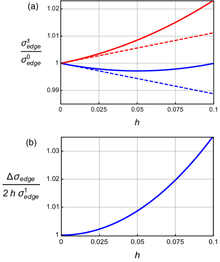
Figure 2: Comparison of the exact edge domain wall energies in Eq. (III) with the approximate ones given by Eq. (17) for $Q=1.674$ and $\kappa=0.366$ (see Sec. VI for the corresponding material parameters. For those parameters, the value of $h=0.1$ corresponds to $\mu_{0}H=132$ mT). (a) Blue and red curves correspond to $\sigma_{edge}^{+}$ and $\sigma_{edge}^{-}$, respectively. Solid lines correspond to the exact values from Eq. (III) and dashed lines represent the approximation of Eq. (17). (b) The relative error in approximating $\Delta\sigma_{edge}=\sigma_{edge}^{+}-\sigma_{edge}^{-}$ using Eq. (17) is shown.

We now derive Eq. (12). Close to $y=\pm\tfrac{1}{2}w$ the solutions of Eqs. (8) and (9) approaching $\theta_{h}$ in the sample interior are expected to be well approximated by those on half-line approaching $\theta_{h}$ far from the edge. After a straightforward integration, we obtain $\theta(y)\simeq\theta^{\pm}(y\mp\tfrac{1}{2}w)$, whereGoussev et al. (2013)

$$\theta^{\pm}(y) =2\tan^{-1}\Bigg{(}\tan\left(\frac{\theta_{h}}{2}\right)$$

$$\quad+\frac{\cos(\theta_{h})\sec^{2}\left(\frac{\theta_{h}}{2}\right)}{\tan\left(\frac{\theta_{h}}{2}\right)\mp e^{\mp\sqrt{Q-1}(y-y_{0}^{\pm})\cos(\theta_{h})}}\Bigg{)}.$$ (13)

The unknown values of $y_{0}^{\pm}$ are obtained by substituting the above expression into Eq. (9), yielding

$$y_{0}^{\pm}=\pm\frac{\cosh^{-1}\left(\frac{2\sqrt{Q-1}\cos^{2}\theta_{h}}{\kappa}\pm\sin\theta_{h}\right)}{\cos\theta_{h}\sqrt{Q-1}}.$$ (14)

Introducing $\theta_{0}^{\pm}=\theta^{\pm}(0)$, where, after simplifying the obtained expressions, one gets explicitly

$$\theta_{0}^{\pm}=\arcsin\left(\sin\theta_{h}\mp{\kappa\over 2\sqrt{Q-1}}\right).$$ (15)

We can then compute the contributions of the profiles in Eq. (III) by plugging them into the energy in Eq. (III). After a rather tedious calculation, up to an exponentially small error $g_{0}(h,w)$ we obtain Eq. (12) with $\sigma_{edge}^{\pm}$ given explicitly by

$$\sigma_{edge}^{\pm} =2\sqrt{Q-1}\big{(}\theta_{h}\sin\theta_{h}+\cos\theta_{h}$$

$$\quad-\cos\theta_{0}^{\pm}-\theta_{0}^{\pm}\sin\theta_{h}\big{)}\pm\kappa(\theta_{0}^{\pm}-\theta_{h}).$$ (16)

Focusing on the regime of moderate values of $h\lesssim 1$, which is the main regime of practical interest, linearizing Eq. (III) in $h$ we get

$$\sigma_{edge}^{\pm}\simeq\sigma_{edge}^{0}\pm\sigma_{edge}^{1}h,\qquad 0<h\lesssim 1,$$ (17)

where

$$\sigma_{edge}^{0} =2\sqrt{Q-1}\left(1-\sqrt{1-{\kappa^{2}\over 4(Q-1)}}\,\right)$$

$$\quad\qquad\quad\qquad-\kappa\arcsin\left({\kappa\over 2\sqrt{Q-1}}\right),$$ (18)

$$\sigma_{edge}^{1} ={2\over\sqrt{Q-1}}\arcsin\left({\kappa\over 2\sqrt{Q-1}}\right)-{\kappa\over Q-1}.$$ (19)

We note that Eqs. (17) gives a very good approximation to the exact expression in Eq. (III), see Fig. 2(a). In fact, the difference $\sigma_{edge}^{+}-\sigma_{edge}^{-}$, which is the relevant quantity for the domain wall tilt, is captured by Eq. (III) within a few percent for practically all values of $h$ and $\kappa$, see Fig. 2(b).

Before concluding this section, we make several observations regarding Eq. (17). First, as expected, $\sigma_{edge}^{0,1}\to 0$ as $\kappa\to 0$, indicating that the edge domain walls disappear without DMI irrespectively of the magnitude of $h$. Of course, the same conclusion holds for Eq. (III) as well. Second, for $h\lesssim 1$ the applied field affects the contribution of the edge domain walls to the energy only through $\sigma_{edge}^{1}$. At the same time, it easy to see that as a function of $\kappa$ we have $\sigma_{edge}^{1}=O(\kappa^{3})$, indicating that the effect of the edge walls is negligible when the surface DMI is sufficiently weak.

IV One-dimensional interior wall profile

We now turn to interior walls and obtain the leading order expressions for the one-dimensional wall profiles and their energies as functions of the wall orientation for $h\lesssim 1$. We focus mostly on the two relevant cases that are amenable to an analytical treatment: $h\ll\kappa\sim 1$ and $h\sim\kappa\ll 1$, even though our method is applicable to all values of the parameters $\kappa$ and $h$ for which Dzyaloshinskii walls are expected to exist. For notational convenience, we introduce the constant two-dimensional vector

$$\overline{\mathbf{m}}_{\perp}=(Q-1)^{-1}h\hat{\mathbf{y}},$$ (20)

equal to the in-plane component of the equilibrium magnetization in the film bulk.

We consider a one-dimensional profile in the direction $\mathbf{n}_{\alpha}=(\cos\alpha,\sin\alpha)$, namely, a magnetization configuration $\mathbf{m}(\xi)=(\mathbf{m}_{\perp}(\xi),m_{\parallel}(\xi))$, where $\xi=\mathbf{r}\cdot\mathbf{n}_{\alpha}$. Then from Eq. (II) with $w=\infty$ the energy per unit length of the wall profile $\mathbf{m}(\xi)$ is

$$\!\!\!\!\!\!E_{\alpha}(\mathbf{m})\!\! = \!\!\int_{-\infty}^{\infty}\Big{[}|\mathbf{m}^{\prime}|^{2}+(Q-1)|\mathbf{m}_{\perp}-\overline{\mathbf{m}}_{\perp}|^{2}$$ (21)

$$\!+\kappa\left(m_{\parallel}(\mathbf{n}_{\alpha}\cdot\mathbf{m}_{\perp}^{\prime})-m_{\parallel}^{\prime}(\mathbf{m}_{\perp}\cdot\mathbf{n}_{\alpha})\right)\Big{]}d\xi.$$

The profile is to satisfy the following conditions at infinity:

$$\mathbf{m}_{\perp}(\pm\infty)=\overline{\mathbf{m}}_{\perp},\qquad m_{\parallel}(\pm\infty)=\pm\sqrt{1-|\overline{\mathbf{m}}_{\perp}|^{2}},$$ (22)

and the associated Euler-Lagrange equation is

$$\mathbf{m}_{\perp}^{\prime\prime}-(Q-1)(\mathbf{m}_{\perp}-\overline{\mathbf{m}}_{\perp})+\kappa m_{\parallel}^{\prime}\mathbf{n}_{\alpha} =\lambda(\xi)\mathbf{m}_{\perp},$$ (23)

$$m_{\parallel}^{\prime\prime}-\kappa(\mathbf{n}_{\alpha}\cdot\mathbf{m}_{\perp}^{\prime}) =\lambda(\xi)m_{\parallel},$$ (24)

where $\lambda(\xi)$ is a scalar Lagrange multiplier due to the pointwise unit length constraint on $\mathbf{m}$. The wall energy $\sigma_{wall}$ associated with a solution $\mathbf{m}=\mathbf{m}^{\alpha}(\xi)$ of Eqs. (23) and (24) satisfying (22) is defined as

$$\sigma_{wall}(\alpha)=E_{\alpha}(\mathbf{m}^{\alpha}).$$ (25)

A distinctive feature of the wall energy in Eq. (25) is that for $\kappa\not=0$ it depends on the wall orientation $\mathbf{n}_{\alpha}$.

It is not possible to find an analytical solution to the system of Eqs. (22)–(24) for general values of $Q$, $\kappa$, $h$, and $\alpha$. Although it is not difficult to construct such solutions numerically for any given set of the parameters (see Sec. VI).

IV.1 $h\ll\kappa\sim 1$ regime

We now wish to obtain the leading order expansion of $\sigma_{wall}(\alpha)$ for $h\ll 1$ and $\kappa\sim 1$. Setting $h=0$ in Eqs. (23) and (24) yields the equation for the profile $\mathbf{m}_{0}=\mathbf{m}_{0}(\xi)$:

$$\mathbf{m}_{0,\perp}^{\prime\prime}-(Q-1)\mathbf{m}_{0,\perp}+\kappa m_{0,\parallel}^{\prime}\mathbf{n}_{\alpha} =\lambda_{0}(\xi)\mathbf{m}_{0,\perp},$$ (26)

$$m_{0,\parallel}^{\prime\prime}-\kappa(\mathbf{n}_{\alpha}\cdot\mathbf{m}_{0,\perp}^{\prime}) =\lambda_{0}(\xi)m_{0,\parallel}.$$ (27)

The solution of Eqs. (26) and (27) that satisfies (22) is explicitly given by

$$\begin{split}\mathbf{m}_{0}(\xi)&=(\mathbf{n}_{\alpha}\sin\theta_{0}(\xi),\cos\theta_{0}(\xi)),\\ \theta_{0}(\xi)&=2\arctan e^{-\xi\sqrt{Q-1}},\end{split}$$ (28)

and for $h=0$ we have $E_{\alpha}(\mathbf{m}_{0})=\sigma_{wall}^{0}$, where

$$\sigma_{wall}^{0} =4\sqrt{Q-1}-\pi\kappa.$$ (29)

Notice that $\sigma_{wall}^{0}$ does not depend on $\alpha$.

To obtain the leading order correction to $\sigma_{wall}^{0}$, we write $\mathbf{m}^{\alpha}=\mathbf{m}_{0}+\mathbf{m}_{1}$, where $|\mathbf{m}_{1}|\ll|\mathbf{m}_{0}|=1$, and note that due to the pointwise unit length constraint, we have $\mathbf{m}_{0}\cdot\mathbf{m}_{1}\simeq 0$ to the leading order. Next, we substitute this expansion into Eq. (21) to obtain, keeping only the terms that are linear in $\mathbf{m}_{1}$ and $\overline{\mathbf{m}}_{\perp}$:

$$\sigma_{wall} (\alpha)\simeq\sigma_{wall}^{0}+\int_{-\infty}^{\infty}\Big{[}2\mathbf{m}_{0}^{\prime}\cdot\mathbf{m}_{1}^{\prime}$$

$$\,\,\qquad+2(Q-1)\mathbf{m}_{0,\perp}\cdot(\mathbf{m}_{1,\perp}-\overline{\mathbf{m}}_{\perp})$$

$$\,\,\qquad+\kappa\Big{(}m_{0,\parallel}(\mathbf{n}_{\alpha}\cdot\mathbf{m}_{1,\perp}^{\prime})+m_{1,\parallel}(\mathbf{n}_{\alpha}\cdot\mathbf{m}_{0,\perp}^{\prime})$$

$$\,\,\qquad-(\mathbf{n}_{\alpha}\cdot\mathbf{m}_{0,\perp})m_{1,\parallel}^{\prime}-(\mathbf{n}_{\alpha}\cdot\mathbf{m}_{1,\perp})m_{0,\parallel}^{\prime}\Big{)}\Big{]}\,d\xi.$$ (30)

Integrating by parts and using Eq. (22), this expression may be rewritten equivalently as

$$\sigma_{wall}(\alpha)\simeq\sigma_{wall}^{0}+2\kappa\mathbf{n}_{\alpha}\cdot\overline{\mathbf{m}}_{\perp}$$

$$\quad-2(Q-1)\int_{-\infty}^{\infty}\mathbf{m}_{0,\perp}\cdot\overline{\mathbf{m}}_{\perp}d\xi$$

$$\quad-2\int_{-\infty}^{\infty}\Big{[}\mathbf{m}_{0}^{\prime\prime}\cdot\mathbf{m}_{1}-(Q-1)\mathbf{m}_{0,\perp}\cdot\mathbf{m}_{1,\perp}$$

$$\quad-\kappa\Big{(}m_{1,\parallel}(\mathbf{n}_{\alpha}\cdot\mathbf{m}_{0,\perp}^{\prime})-(\mathbf{n}_{\alpha}\cdot\mathbf{m}_{1,\perp})m_{0,\parallel}^{\prime}\Big{)}\Big{]}\,d\xi.$$ (31)

In fact, in the above formula the integrand in the last integral is zero to the leading order, which can be seen by multiplying both sides of the Euler-Lagrange equation in Eqs. (26) and (27) by $\mathbf{m}_{1}$ and using the condition $\mathbf{m}_{0}\cdot\mathbf{m}_{1}=0$ to the leading order in $h$. Thus, substituting the profile $\mathbf{m}_{0}$ into the above expression, after some more algebra we get that the wall energy up to $O(h^{2})$ is

$$\sigma_{wall}(\alpha)\simeq\sigma_{wall}^{0}-\sigma_{wall}^{1}h\sin\alpha,$$ (32)

where

$$\sigma_{wall}^{1} =\frac{2\pi}{\sqrt{Q-1}}-\frac{2\kappa}{Q-1}.$$ (33)

We point out that the obtained expression for $\sigma_{wall}(\alpha)$ appears to be meaningless when $\kappa=0$, since Eq. (33) suggests that for $h>0$ the wall energy depends on the angle $\alpha$ even in the absence of DMI. Yet the energy in Eq. (21) is manifestly independent of $\alpha$. The reason for this discrepancy is the fact that our approximations are justified only when $\kappa\sim 1\gg h$, while the limit of $\kappa\to 0$ with $h>0$ fixed violates this assumption. In fact, when $\kappa\sim 1$ the magnetization in a domain wall rotates mostly in the plane spanned by $\mathbf{n}_{\alpha}$ and $\hat{\mathbf{z}}$, while when $\kappa=0$ the magnetization would prefer to rotate in the plane spanned by $\hat{\mathbf{y}}$ and $\hat{\mathbf{z}}$, even if $\mathbf{n}_{\alpha}\not=\hat{\mathbf{y}}$. To resolve this discrepancy, we need to consider the case of $\kappa\lesssim h\ll 1$ separately.

IV.2 $h\sim\kappa\ll 1$ regime

When both $h$ and $\kappa$ are small and comparable, we can further simplify the argument above to obtain the following equation for $\mathbf{m}_{0}$ in place of Eqs. (26) and (27) to the leading order:

$$\mathbf{m}_{0,\perp}^{\prime\prime}-(Q-1)\mathbf{m}_{0,\perp} =\lambda_{0}(\xi)\mathbf{m}_{0,\perp},$$ (34)

$$m_{0,\parallel}^{\prime\prime} =\lambda_{0}(\xi)m_{0,\parallel}.$$ (35)

The solution of Eqs. (34) and (35) that satisfies (22) is explicitly given by $\mathbf{m}_{0}=\mathbf{m}_{0}^{\mathbf{n}}$, where

$$\begin{split}\mathbf{m}_{0}^{\mathbf{n}}(\xi)&=(\mathbf{n}\sin\theta_{0},\cos\theta_{0}),\\ \theta_{0}(\xi)&=2\arctan e^{-\xi\sqrt{Q-1}},\end{split}$$ (36)

and $\mathbf{n}\in\mathbb{R}^{2}$ is an arbitrary constant unit vector. For $h=\kappa=0$ we have $E_{\alpha}(\mathbf{m}_{0}^{\mathbf{n}})=\sigma_{wall}^{0}$, where

$$\sigma_{wall}^{0} =4\sqrt{Q-1}.$$ (37)

Notice that $\sigma_{wall}^{0}$ does not depend on $\alpha$ or $\mathbf{n}$ and coincides with the energy of the Néel wall in the absence of nonlocal effects.

Now, writing again $\mathbf{m}^{\alpha}=\mathbf{m}_{0}^{\mathbf{n}}+\mathbf{m}_{1}$ and expanding the energy to the next order in $h$ and $\kappa$, we obtain

$$\!\!E_{\alpha}(\mathbf{m})\!\! \simeq\!\! \sigma_{wall}^{0}+\int_{-\infty}^{\infty}\Big{[}2\mathbf{m}_{0}^{\prime}\cdot\mathbf{m}_{1}^{\prime}$$ (38)

$$+\kappa\left(m_{0,\parallel}(\mathbf{n}_{\alpha}\cdot\mathbf{m}_{0,\perp}^{\prime})-m_{0,\parallel}^{\prime}(\mathbf{m}_{0,\perp}\cdot\mathbf{n}_{\alpha})\right)$$

$$+2(Q-1)\mathbf{m}_{0,\perp}\cdot(\mathbf{m}_{1,\perp}-\overline{\mathbf{m}}_{\perp})\Big{]}d\xi,$$

and following the same arguments as in Sec. IV.1 we arrive at

$$E_{\alpha}(\mathbf{m})=\sigma_{wall}^{0}-\frac{2\pi h}{\sqrt{Q-1}}({\mathbf{n}}\cdot\hat{\mathbf{y}})-\pi\kappa({\mathbf{n}}\cdot\mathbf{n}_{\alpha}).$$ (39)

Finally, in order to find the direction of vector $\mathbf{n}$ we need to minimize the above energy with respect to $\mathbf{n}$. It is easy to see that

$${\mathbf{n}}=\frac{2\pi h\hat{\mathbf{y}}+\pi\kappa\mathbf{n}_{\alpha}\sqrt{Q-1}}{\left|2\pi h\hat{\mathbf{y}}+\pi\kappa\mathbf{n}_{\alpha}\sqrt{Q-1}\right|}$$ (40)

minimizes the right-hand side of Eq. (39), and the minimum of the energy is given by

$$\!\!\!\!\!\!\!\!\sigma_{wall}(\alpha)\!\! \simeq\!\! 4\sqrt{Q-1}$$ (41)

$$-\pi\sqrt{\kappa^{2}\cos^{2}\alpha+\left(\kappa\sin\alpha+\frac{2h}{\sqrt{Q-1}}\right)^{2}}.$$

Thus, the obtained magnetization profile rotates mostly in the plane spanned by $\mathbf{n}$ and $\hat{\mathbf{z}}$, with $\mathbf{n}$ depending sensitively on both $h$ and $\kappa$. Furthermore, the obtained result is consistent with the one of Sec. IV.1. Indeed, expanding the expression in Eq. (41) in the powers of $h$ with $\kappa\ll 1$ fixed yields Eq. (32) to linear order in $h$ and the leading order in $\kappa$. At the same time, setting $\kappa=0$ with $0<h\ll 1$ fixed in Eq. (39), we recover the wall energy $\sigma_{wall}\simeq 4\sqrt{Q-1}-{2\pi h\over\sqrt{Q-1}}$, which is easily seen to be the wall energy for a profile rotating in the plane spanned by $\hat{\mathbf{y}}$ and $\hat{\mathbf{z}}$, consistent with the discussion at the end of Sec. IV.1.

V Two-dimensional problem

Figure 3: Schematics of a general domain wall geometry in an infinite strip. The up/down symbols indicate the direction of the magnetization far from the wall and the strip edges.

We now demonstrate how the information about one-dimensional domain walls obtained in the preceding sections may be applied to a single Dzyaloshinskii domain wall running across an infinite ferromagnetic nanostrip. For an illustration of the geometry, see Fig. 3, where the domain wall is represented by a thick solid curve. Here we wish to treat the wall as a one-dimensional object, whose shape is determined by minimizing an appropriate geometric energy functional. This energy functional is obtained via a suitable asymptotic reduction of the two-dimensional micromagnetic energy in Eq. (II). For a rigorous justification of such an approach in a closely related context, see Ref. Muratov and Slastikov, 2016.

Using Eq. (12), we can rewrite Eq. (II) in the following way:

$$E(\mathbf{m}) =\int_{-\infty}^{\infty}\int_{-w/2}^{w/2}\Big{[}|\nabla\mathbf{m}|^{2}+(Q-1)|\mathbf{m}_{\perp}-\overline{\mathbf{m}}_{\perp}|^{2}$$

$$-w^{-1}(\sigma_{edge}^{+}+\sigma_{edge}^{-})-w^{-1}g_{0}(h,w)$$

$$+\kappa\left(m_{\parallel}\nabla\cdot\mathbf{m}_{\perp}-\mathbf{m}_{\perp}\cdot\nabla m_{\parallel}\right)\Big{]}\,d^{2}r.$$ (42)

Recall that $\overline{\mathbf{m}}_{\perp}$ was defined in Eq. (20). We next consider a domain wall whose shape is described by a smooth curve $\gamma$ which is the graph of a function $u:(-w/2,w/2)\to\mathbb{R}$, i.e., for every $\mathbf{r}\in\gamma$ we have $\mathbf{r}=(u(y),y)$ for some $y\in(-w/2,w/2)$. The associated magnetization profile ${\mathfrak{m}}_{\gamma}$ in the vicinity of this curve will then be close to the optimal one-dimensional interior wall profile analyzed in Sec. IV. Let $\mathbf{r}$ be a point in the vicinity of $\gamma$ and let $\mathbf{r}_{\gamma}$ be the orthogonal projection of $\mathbf{r}$ on $\gamma$. Denote by $\mathbf{n}_{\alpha}(\mathbf{r}_{\gamma})=(\cos\alpha(\mathbf{r}_{\gamma}),\sin\alpha(\mathbf{r}_{\gamma}))$ the unit normal vector to $\gamma$ at point $\mathbf{r}_{\gamma}$ pointing towards the region where $m_{\parallel}>0$, with $\alpha(\mathbf{r}_{\gamma})$ the angle that the normal vector $\mathbf{n}_{\alpha}(\mathbf{r}_{\gamma})$ makes with the $x$-axis at point $\mathbf{r}_{\gamma}$. Then the magnetization profile $\mathbf{m}={\mathfrak{m}}_{\gamma}$ associated with the curve $\gamma$ is expected to satisfy

$${\mathfrak{m}}_{\gamma}(\mathbf{r})\simeq\mathbf{m}^{\alpha}((\mathbf{r}-\mathbf{r}_{\gamma})\cdot\mathbf{n}_{\alpha}(\mathbf{r}_{\gamma})),$$ (43)

where $\mathbf{m}^{\alpha}$ is the optimal profile that minimizes the one-dimensional interior wall energy $E_{\alpha}$ in Eq. (21). Assuming that the curvature of $\gamma$ does not exceed $O(w^{-1})$, the contribution to the energy by the neighborhood of $\gamma$ for $w\gg 1$ is then dominated by the one-dimensional wall energy $E_{\alpha}(\mathbf{m}^{\alpha})$ integrated over $\gamma$, which by Eq. (25) is

$$E_{int}({\mathfrak{m}}_{\gamma})=\int_{\gamma}\sigma_{wall}(\alpha(\mathbf{r}))ds(\mathbf{r}),$$ (44)

where $ds$ is the arclength differential along $\gamma$. Thus, the energy of the interior wall is characterized by an anisotropic line tension.

Away from the interior wall the magnetization obeys

$$\mathfrak{m}_{\gamma}\simeq\left(\overline{\mathbf{m}}_{\perp},\pm\sqrt{1-|\overline{\mathbf{m}}_{\perp}|^{2}}\right),$$ (45)

consistently with Eq. (43). However, this relation is violated close to the strip edges, where edge domain walls appear. Therefore, we also need to take into account the edge domain wall profiles analyzed in Sec. III in those regions. Accordingly, one expects

$$\mathfrak{m}_{\gamma}\simeq(0,\sin(\theta^{+}(y-\tfrac{1}{2}w)),\cos(\theta^{+}(y-\tfrac{1}{2}w))),$$ (46)

for $x>u(w/2)$ and $y\sim w/2$, whereas

$$\mathfrak{m}_{\gamma}\simeq(0,\sin(\theta^{-}(y+\tfrac{1}{2}w)),\cos(\theta^{-}(y+\tfrac{1}{2}w))),$$ (47)

for $x>u(-w/2)$ and $y\sim-w/2$. Similarly, in view of the symmetry relation given by Eq. (10), we also find

$$\mathfrak{m}_{\gamma}\simeq(0,\sin(\theta^{-}(\tfrac{1}{2}w-y)),\cos(\theta^{-}(\tfrac{1}{2}w-y))),$$ (48)

for $x<u(w/2)$ and $y\sim w/2$, whereas

$$\mathfrak{m}_{\gamma}\simeq(0,\sin(\theta^{+}(-\tfrac{1}{2}w-y)),\cos(\theta^{+}(-\tfrac{1}{2}w-y))),$$ (49)

for $x<u(-w/2)$ and $y\sim-w/2$. The corresponding edge wall energy is then

$$E_{edge}(\mathfrak{m}_{\gamma})=(\sigma_{edge}^{+}-\sigma_{edge}^{-})(u(-w/2)-u(w/2)),$$ (50)

recalling that we subtracted the contribution of $\sigma_{edge}^{+}+\sigma_{edge}^{-}$ in Eq. (V). Finally, to match the interior and the edge wall profiles near points $x=u(\pm\tfrac{1}{2}w)$ and $y=\pm\tfrac{1}{2}w$, one uses the construction from Ref. Muratov and Slastikov, 2016, which can be seen not to contribute to the energy to the leading order.

Putting all the leading order contributions to the energy in Eq. (V) together, we obtain

$$E(\mathfrak{m}_{\gamma})\simeq E_{int}(\mathfrak{m}_{\gamma})+E_{edge}(\mathfrak{m}_{\gamma}).$$ (51)

Then, using the parametrization $x=u(y)$ of the curve $\gamma$, we find explicitly

$$E(\mathfrak{m}_{\gamma}) \simeq\int_{-w/2}^{w/2}\sigma_{wall}\big{(}-\arctan u^{\prime}(y)\big{)}\sqrt{1+|u^{\prime}(y)|^{2}}\,dy$$

$$\quad-(\sigma_{edge}^{+}-\sigma_{edge}^{-})(u(w/2)-u(-w/2)),$$ (52)

where we recall that $\alpha(\mathbf{r})=-\arctan u^{\prime}(y)$.

As is well knownHerring (1952) and can be easily seen directly from Eq. (V), every critical point $\gamma$ of $\gamma\mapsto E(\mathfrak{m}_{\gamma})$ is a straight line. In particular, minimizers of $E(\mathfrak{m}_{\gamma})$ are straight domain walls running across the strip. Thus, the only free parameter in the problem is the difference between the $x$-positions $u(w/2)-u(-w/2)$ of the wall at the top and bottom edges. In fact, from the dimensional considerations this difference is proportional to $w$, i.e., $w$ can be scaled out of the energy. Thus, the only free parameter of the minimization problem for $E(\mathfrak{m}_{\gamma})$ is the tilt angle $\beta\in(-{\pi\over 2},{\pi\over 2})$ that the line $\gamma=\gamma_{\beta}$ makes with the $y$-axis. Note that this angle coincides with the angle $\alpha$ defining the normal vector $\mathbf{n}_{\alpha}$ of $\gamma_{\beta}$. To compute the tilt angle, we substitute the straight line ansatz $\gamma_{\beta}$ into Eq. (V), and the angle is then obtained by minimizing the expression

$${E(\mathfrak{m}_{\gamma_{\beta}})\over w}\simeq{\sigma_{wall}(\beta)\over\cos\beta}+(\sigma_{edge}^{+}-\sigma_{edge}^{-})\tan\beta.$$ (53)

over $\beta$, which completely characterizes existence and multiplicity of tilted domain walls in the presence of DMI. It is clear from Eq. (53) that the equilibrium tilt angle is independent of the strip width and depends only on the dimensionless material parameters $\kappa$ and $Q$ and the dimensionless applied field strength $h$. In fact, dimensional analysis shows that the equilibrium tilt angle depends on these parameters only via two combinations, $\kappa/\sqrt{Q-1}$ and $h/(Q-1)$.

To conclude this section, we note that, as expected, the tilt angle becomes zero when the effect of the DMI vanishes. This can be readily seen from Eq. (53), taking into account that for $\kappa=0$ we have $\sigma_{edge}^{+}=\sigma_{edge}^{-}$ and $\sigma_{wall}$ becomes independent of $\beta$, see Eqs. (III) and (21).

In the rest of this section, we consider two parameter regimes based on analytical results presented in Sec. IV.1 and IV.2 for which explicit expressions for the tilt can be obtained.

V.1 $h\ll\kappa\sim 1$ regime

In this regime, an approximate expression for $\sigma_{wall}(\alpha)$ is given by Eqs. (29), (32) and (33), and $\sigma_{edge}^{\pm}$ are given by Eqs. (17)–(19). Substituting these expressions into Eq. (53), we obtain

$${E(\mathfrak{m}_{\gamma_{\beta}})\over w}\simeq{\sigma_{wall}^{0}\over\cos\beta}+h(2\sigma_{edge}^{1}-\sigma_{wall}^{1})\tan\beta.$$ (54)

Minimizing this expression yields the unique equilibrium tilt angle

$$\beta=\arcsin\left({\sigma_{wall}^{1}-2\sigma_{edge}^{1}\over\sigma_{wall}^{0}}\,h\right).$$ (55)

In particular, since we are in the regime of small applied fields the equilibrium tilt angle is linear in $h$:

$$\beta\simeq{4h\arccos\left({\kappa\over 2\sqrt{Q-1}}\right)\over 4(Q-1)-\pi\kappa\sqrt{Q-1}}.$$ (56)

This formula is one of the main findings of our paper.

We note that the expression in Eq. (55) formally coincides with the formula for the contact angle of a triple junction between three distinct phasesLandau and Lifshits (1980). Nevertheless, in addition to the contribution of the difference of line tensions $\sigma_{edge}^{0}\pm\sigma_{edge}^{1}h$ associated with the two edges, the formula also contains a contribution $\sigma_{wall}^{1}$ due to anisotropy of the line tension of Dzyaloshinskii wall.

V.2 $h\sim\kappa\ll 1$ regime

In this regime, the explicit expressions for $\sigma_{wall}(\alpha)$ is given by Eq. (41). At the same time, recalling that the expression for $\sigma_{edge}^{\pm}$ in Eq. (17) remains valid also for $\kappa\ll 1$ and that $\sigma_{edge}^{1}=O(\kappa^{3})$, one can see that the contribution of $\sigma_{edge}^{+}-\sigma_{edge}^{-}$ in Eq. (53) is negligible. Thus, to the leading order we arrive at

$${E(\mathfrak{m}_{\gamma_{\beta}})\over w} \simeq\frac{4\sqrt{Q-1}}{\cos\beta}$$

$$\quad-\pi\sqrt{\kappa^{2}+\left(\kappa\tan\beta+\frac{2h}{\sqrt{Q-1}\,\cos\beta}\right)^{2}}.$$ (57)

Note that the second term in Eq. (57) is a small perturbation for the first term, which is a convex even function of $\beta$ approaching infinity as $\beta\to\pm{\pi\over 2}$. Therefore, the minimum in Eq. (57) is attained for $|\beta|\ll 1$.

To proceed further, we expand the right-hand side of Eq. (57) in a Taylor series in $\beta$ up to second order and keep only the leading terms in $h$ and $\kappa$. The result is

$${E(\mathfrak{m}_{\gamma_{\beta}})\over w} \simeq 4\sqrt{Q-1}-{2\pi h\kappa\beta\over\sqrt{4h^{2}+\kappa^{2}(Q-1)}}$$

$$\quad+\beta^{2}\left(2\sqrt{Q-1}-\frac{\pi\kappa}{2}\right).$$ (58)

Minimizing this expression in $\beta$ yields the equilibrium tilt angle

$$\beta\simeq\frac{\pi h\kappa}{\left(2\sqrt{Q-1}-\frac{\pi\kappa}{2}\right)\sqrt{4h^{2}+\kappa^{2}(Q-1)}}.$$ (59)

This formula is another main finding of our paper. As expected, the title angle in Eq. (59) goes to zero as $h\to 0$. Moreover, for $h\ll\kappa\ll 1$ we obtain an interesting result:

$$\beta\simeq{\pi h\over 2(Q-1)},\qquad h\ll\kappa,$$ (60)

i.e., the equilibrium tilt angle becomes independent of the DMI strength. In fact, this is in agreement with the prediction of Eq. (56) for vanishingly small $\kappa$.

Similarly, when $\kappa\ll h\ll 1$, we find another surprising result:

$$\beta\simeq{\pi\kappa\over 4\sqrt{Q-1}},\qquad\kappa\ll h,$$ (61)

i.e., the equilibrium tilt angle becomes independent of the applied field. This indicates that for moderate values of the DMI strength the measured tilt angle may be used to directly assess the value of the interfacial DMI constant experimentally.

VI Comparison with micromagnetic simulations

To validate the conclusions of our analysis, we performed three types of numerical tests. For the material parameters, we chose those of a 0.6 nm-thick film corresponding roughly to two monolayers of Co, with parameters $A=10^{-11}$J/m, $K=1.25\times 10^{6}$ J/m³, $M_{s}=1.09\times 10^{6}$ A/m. The representative values of the DMI strength and applied field are $D=1$ mJ/m² and $\mu_{0}H=100$ mT, respectivelyBoulle et al. (2013).

We begin by comparing the tilted Dzyaloshinskii domain wall profiles from the two-dimensional numerical simulations obtained using Mumax3 simulation package within the local approximation of the magnetostatic energy [as in Eq. (II)], with the 1D domain wall profiles $\mathbf{m}^{\alpha}$ minimizing $E_{\alpha}$ in Eq. (21). In the micromagnetic simulations, we used a conservative discretization step of $1$ nm in the $xy$-plane. To obtain the one-dimensional profiles $\mathbf{m}^{\alpha}$ minimizing $E_{\alpha}$, we solved Eqs. (22)–(24) by writing $\mathbf{m}^{\alpha}$ in polar coordinates for $\theta$ and $\phi$:

$$\mathbf{m}^{\alpha}=(\sin\theta\cos\phi,\sin\theta\sin\phi,\cos\theta),$$ (62)

and solving the following evolution problem:

$$\theta_{t} =\theta_{\xi\xi}-\left(\phi_{\xi}^{2}+Q-1\right)\sin\theta\cos\theta+h\cos\theta\sin\phi$$

$$\quad-\kappa\phi_{\xi}\sin(\phi-\alpha)\sin^{2}\theta,$$ (63)

$$\phi_{t} =\phi_{\xi\xi}+2\theta_{\xi}\phi_{\xi}\cot\theta+h\csc\theta\cos\phi$$

$$\quad+\kappa\theta_{\xi}\sin(\phi-\alpha),$$ (64)

until a steady state was reached. Here the subscripts stand for the respective partial derivatives. The equations above correspond to an overdamped Landau-Lifshitz-Gilbert equation, and their steady states solve Eqs. (23) and (23) upon substitution into Eq. (62). Also, in terms of $\theta$ and $\phi$ the wall energy is

$$E_{\alpha}(\mathbf{m}^{\alpha}) =\int_{-\infty}^{\infty}\bigg{(}\theta_{\xi}^{2}+\phi_{\xi}^{2}\sin^{2}\theta+(Q-1)\sin^{2}\theta$$

$$\quad-2h\sin\theta\sin\phi+{h^{2}\over Q-1}+\kappa\theta_{\xi}\cos(\phi-\alpha)$$

$$\quad-\kappa\phi_{\xi}\sin(\phi-\alpha)\cos\theta\sin\theta\bigg{)}d\xi.$$ (65)

The parameters at the beginning of this section correspond to the dimensionless parameters $Q=1.674$, $\kappa=0.366$ and $h=0.073$. For these parameters, we carried out Mumax3Vansteenkiste et al. (2014) simulations in an 800 nm $\times$ 400 nm strip, which corresponds to $w=109\gg 1$, and obtained the magnetization profile with the tilt angle $\beta\simeq 11.2^{\circ}$. We then solved Eqs. (63) and (64) with $\alpha=11.2^{\circ}$ and obtained the optimal one-dimensional wall profile $\mathbf{m}^{\alpha}$. The result of the two-dimensional computation is compared with the one-dimensional profile in Fig. 4, which plots the $z$-component of the two-dimensional profile $\mathbf{m}$ along the $x$-axis alongside with the corresponding section of the optimal profile $\mathfrak{m}_{\gamma_{\alpha}}$ obtained from $\mathbf{m}^{\alpha}$. One can see an almost perfect agreement between the full two-dimensional simulation result and the theoretical prediction of Sec. IV. The same agreement is also observed in the other two components of the magnetization (not shown). This justifies the main premise of our theory about the one-dimensional character of the interior wall profiles.

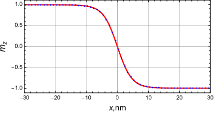
Figure 4: A one-dimensional $y=0$ cut through the computed two-dimensional profile $\mathbf{m}$ (blue dots) vs. a one-dimensional cut through the optimal profile $\mathfrak{m}_{\gamma_{\alpha}}$ (red line). See text for details.

To further test the conclusions of our theory, we computed the energy $\sigma_{wall}(\alpha)$ of the interior walls as a function of their orientation angle $\alpha$ from the solutions of Eqs. (63) and (64) for the considered values of the parameters. The result is plotted in Fig. 5, along with the analytical approximations given by Eqs. (32) and (41). One can see that both analytical formulas give a fairly good approximation to the exact interior wall energy $\sigma_{wall}(\alpha)$ for these parameters. The agreement becomes much better for smaller values of $h$.

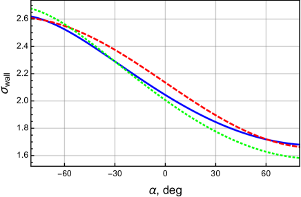
Figure 5: The dependence $\sigma_{wall}(\alpha)$ obtained from the numerical minimization of $E_{\alpha}$ (blue solid curve), the analytical expressions given by Eq. (32) (red dashed curve) and Eq. (41) (green dotted curve), corresponding to the dimensionless parameters $Q=1.674$, $\kappa=0.366$ and $h=0.073$.

We used the interior wall energy $\sigma_{wall}(\alpha)$ obtained numerically to calculate the equilibrium tilt angle by minimizing the energy in Eq. (53) numerically. This resulted in a unique minimizing angle $\beta=11.4^{\circ}$, in excellent agreement with the result of the full two-dimensional simulation. For comparison, the formulas in Eqs. (56) and (59) yield $\beta=12.8^{\circ}$ and $\beta=13.5^{\circ}$, respectively, still in a good agreement with the two-dimensional result, which is reasonable since both these formulas are at the limits of their applicability for the considered parameters.

For lower fields $h$, the agreement with the predictions of the analytical theory becomes much better. We illustrate this by presenting the results of the full two-dimensional numerical simulations against the analytical predictions by Eqs. (56) and (59) for smaller fields in the whole range of values of $\kappa$. Figure 6 shows the dependence of the equilibrium tilt angle $\beta$ on the applied field for several values of the DMI strength. As can be seen from the figure, the agreement between the theory and the numerics rapidly increases as the applied magnetic field or the DMI strength are decreased. This trend can also be seen from the plot of the equilibrium tilt angle as a function of the DMI strength for several value of the applied field shown in Fig. 7.

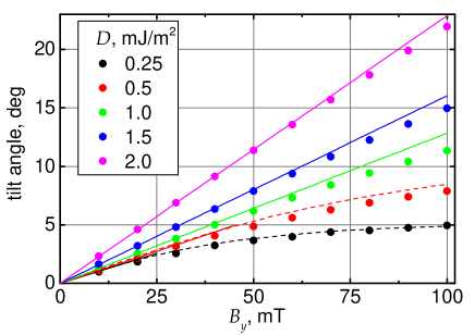
Figure 6: Equilibrium tilt angle, $\beta$, vs. applied field $B_{y}=\mu_{0}H$ for several values of the DMI strength $D$, alongside with the predictions of Eq. (56) (solid lines) and Eq. (59) (dashed lines).

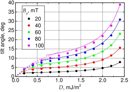
Figure 7: Equilibrium tilt angle, $\beta$, vs. DMI strength $D$ for several values of the applied field $B_{y}=\mu_{0}H$, alongside with the predictions of Eq. (56) (solid lines) and Eq. (59) (dashed lines).

So far we presented the results of micromagnetic simulations for a nanostrip, using a common approximation that neglects the dipolar interaction. Winter (1961); Gioia and James (1997) More precisely, in the preceding simulations, the effect of dipolar interactions was accounted only by introducing a local shape anisotropy term. Let us conclude this section by discussing the results of micromagnetic simulations for thin nanostrips with the full account of magnetostatic interaction. The material parameters and the corresponding dimensionless parameters were the same as in the simulations without the dipolar interactions. The length of the nanostrip was extended $1.5$ times to reduce the effect of magnetic charges at the ends of the nanostrip. The full accounting of the magnetostatic energy in the simulations leads to an increase in the DW tilt angle, see Fig. 8. One can see that for the considered parameters the presence of the dipolar interaction affects the tilt angle relatively weakly for moderate applied fields and DMI strengths. Notably, the impact of the dipolar interaction is practically negligible for sufficiently small DMI strengths, but increases with increasing DMI strength. We attribute this phenomenon to a decrease in the DW stiffness as the value of $\kappa$ is increased, making the domain wall more susceptible to the presence of the dipolar interactions.

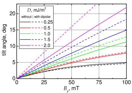
Figure 8: Equilibrium tilt angle, $\beta$, vs. magnetic field $B_{y}$ from simulations with and without the dipolar interactions.

VII Conclusions

We have developed an analytical theory of the Dzyaloshinskii domain wall tilt in a ferromagnetic nanostrip in the perpendicular in-plane magnetic fields. This type of DW tilt is a vivid manifestation of the presence of interfacial DMI in ultrathin ferromagnet/heavy-metal layered structures. Our theory focuses on the geometric aspect of the problem and treats the DW as a curve, whose equilibrium shape is determined by minimizing an appropriate geometric energy functional.

The main ingredients in our theory are the energy densities of edge and interior domain walls. The former are computed explicitly, and the latter can be obtained for any given set of parameters, using a straightforward numerical procedure. We have explicitly considered two regimes: the regime when the dimensionless magnetic field $h$ is much smaller than the dimensionless DMI strength $\kappa$ and the regime when they are both small and comparable. In both regimes, we have found very good agreement with the micromagnetic simulations for the tilt angle.

Our theory has three main findings: First, we derived an exact 1D domain wall profile for any strength of perpendicular in-plane magnetic field. Second, we proved that the DW is always a tilted straight line. Third, this allowed us to obtain an explicit expression for the DW tilt angle. Moreover, in the wide range of DMI strength (as long as DW does not develop yet helicoidal structure), we find that the DW configurations are in general neither Néel nor Bloch type, and that the DW energy is anisotropic (depends on the tilt angle).

In the regime of small fields $h\ll\kappa\lesssim 1$, we have found that the equilibrium angle is proportional to the field strength [Eq. (56)]. On the other hand, for small DMI strengths the tilt angle exhibits a strongly nonlinear dependence on the field strength, even for relatively small fields [Eq. (59)]. Surprisingly, we found that when $h\ll\kappa\ll 1$ the equilibrium tilt angle becomes independent of the DMI strength [Eq. (60)], which can be a good experimental test for our theory. Equally surprisingly, in the opposite regime $\kappa\ll h\ll 1$, we have shown that the equilibrium tilt angle becomes independent of the applied magnetic field [Eq. (61)].

Our results indicate that for moderate DMI strengths the tilt angle may be used to directly assess the value of the interfacial DMI constant experimentally. In other words, our theory gives a method to infer the DMI constant from the tilt angle measurements of the Dzyaloshinskii domain wall. We, therefore, propose an experimental method that requires only a technique for observing the magnetic structure under external field (e.g. Kerr microscopy). To improve the accuracy of the DMI determination, one should measure the tilt angle as a function of magnetic field $B_{y}$, as shown in Fig. 6, and fit this experimental curve to our theory [Eqs. (56) or (59), depending on smallness of the DMI strength relative to the magnetic field].