Production cross sections of hyperons and charmed baryons from $e^{+}e^{-}$ annihilation near $\sqrt{s}=10.52$ GeV

Abstract

We measure the inclusive production cross sections of hyperons and charmed baryons from $e^{+}e^{-}$ annihilation using a 800 fb^-1 data sample taken near the $\Upsilon(4S)$ resonance with the Belle detector at the KEKB asymmetric-energy $e^{+}e^{-}$ collider. The feed-down contributions from heavy particles are subtracted using our data, and the direct production cross sections are presented for the first time. The production cross sections divided by the number of spin states for $S=-1$ hyperons follow an exponential function with a single slope parameter except for the $\Sigma(1385)^{+}$ resonance. Suppression for $\Sigma(1385)^{+}$ and $\Xi(1530)^{0}$ hyperons is observed. Among the production cross sections of charmed baryons, a factor of three difference for $\Lambda_{c}^{+}$ states over $\Sigma_{c}$ states is observed. This observation suggests a diquark structure for these baryons.

I Introduction

Inclusive hadron production from $e^{+}e^{-}$ annihilation has been measured for center-of-mass (CM) energy $\sqrt{s}$ of up to about 200 GeV, and summarized by the Particle Data Group PDG2016 . In $e^{+}e^{-}$ annihilation, hadrons are produced after the $e^{+}e^{-}\rightarrow\gamma^{*}\rightarrow q\bar{q}$ creation in the fragmentation process. The observed production cross sections ($\sigma$) show an interesting dependence on their masses ($m$) and their angular momentum ($J$): $\sigma/(2J+1)\propto\exp(-\alpha m)$, where $\alpha$ is a slope parameter. The relativistic string fragmentation model Andersson_PhysRept reproduces well the angular and momentum distributions of mesons in the fragmentation Andersson_PhysRept . In this model, gluonic strings expand between the initial $q\bar{q}$ pair and many $q\bar{q}$ pairs are created subsequently when the energy in the color field gets too large. These $q\bar{q}$ pairs pick up other $\bar{q}q$ and form mesons in the fragmentation process.

For the baryon production, two models are proposed: the diquark model Andersson_PhysRept and the popcorn model Andersson_PhysicaScripta . In the former, diquark ($qq$) and anti-diquark ($\bar{q}\bar{q}$) pairs are created instead of a $q\bar{q}$. In this model, a quark-quark pair is treated as an effective degree of freedom Anselmino:1993 . In the latter, three uncorrelated quarks are produced by either $q\bar{q}$ creation or diquark pair creation and then form baryons. In Ref. Andersson_PhysicaScripta , the prediction of the production rates by these models were compared, and they found that, for decuplet baryons ($\Delta$ and $\Sigma(1385)$), the prediction by the diquark model is smaller than that by the popcorn model. The production rates measured by ARGUS was compared with these models ARGUS_HYPERON_PLB1987 , however, due to the large feed-down from heavier resonances, the direct comparison between the experimental data and the model prediction was difficult.

In earlier measurements at $\sqrt{s}=10$ GeV and at $\sqrt{s}=90$ GeV, production rates of most non-strange light baryons and hyperons follow an exponential mass dependence with a common slope parameter, but significant enhancements for $\Lambda$ and $\Lambda(1520)$ baryons are observed PDG2016 ; Jaffe_Exotica . These enhancements could be explained by the light mass of the spin-0 diquark in $\Lambda$ baryons Jaffe_Exotica ; Wilczek_diquark . However, the previous measurements of inclusive production cross sections contain feed-down from heavier resonances. In order to compare the direct production cross sections of each baryon, feed-down contributions should be subtracted. Charmed baryons have an additional interest, from the viewpoint of baryon structure: the color-magnetic interactions between the charm quark and the light quarks are suppressed due to the heavy charm quark mass, so that diquark degrees of freedom may be enhanced in the production mechanisms.

In this article, we report the production cross sections of hyperons and charmed baryons using Belle Belle_PTEP data recorded at the KEKB $e^{+}e^{-}$ asymmetric-energy collider KEKB . This high-statistics data sample has good particle identification power. In this article, the direct cross sections of hyperons and charmed baryons are described.

This paper is organized as follows. In Sec. II, the data samples and the Belle detector are described, and the analysis to obtain the production cross sections is presented. In Sec. III, the production cross sections are extracted for each baryon, and the production mechanism and the internal structure of baryons are discussed. Finally, we summarize our results in Sec. IV.

II Analysis

For the study of hyperon production cross sections in the hadronic events from $e^{+}e^{-}$ annihilation, we avoid contamination from $\Upsilon(4S)$ decay by using off-resonance data taken at $\sqrt{s}=10.52$ GeV, which is 60 MeV below the mass of the $\Upsilon(4S)$. In contrast, for charmed baryons, for which the production rates are small, especially for the excited states, we use both off- and on-resonance data, the latter recorded at the $\Upsilon(4S)$ energy ($\sqrt{s}=10.58$ GeV). In this article, we report the production cross sections of $\Lambda$, $\Sigma^{0}$, $\Sigma(1385)^{+}$, $\Lambda(1520)$, $\Xi^{-}$, $\Omega^{-}$, $\Xi(1530)^{0}$, $\Lambda_{c}^{+}$, $\Lambda_{c}(2595)^{+}$, $\Lambda_{c}(2625)^{+}$, $\Sigma_{c}(2455)^{0}$, $\Sigma_{c}(2520)^{0}$, $\Omega_{c}^{0}$, and $\Xi_{c}^{0}$. These particles are reconstructed from charged tracks except for $\Sigma^{0}$. Other ground-state baryons are omitted because their main decay modes contain neutral pions or neutrons. Since the absolute branching fractions for $\Omega_{c}^{0}$ and $\Xi_{c}^{0}$ are unknown, the production cross sections multiplied with the branching fractions are presented.

The Belle detector is a large-solid-angle magnetic spectrometer that consists of a silicon vertex detector (SVD), a central drift chamber (CDC), an array of aerogel threshold Cherenkov counters (ACC), time-of-flight scintillation counters (TOF), and an electromagnetic calorimeter (ECL) composed of CsI(Tl) crystals located inside a superconducting solenoid coil that provides a 1.5 T magnetic field. The muon/$K^{0}_{L}$ subsystem sandwiched within the solenoid’s flux return is not used in this analysis. The detector is described in detail elsewhere AbashianNPA479 ; BrodzickaPTEP04D001 .

This analysis uses the data sets with two different inner detector configurations. A 2.0 cm beampipe and a three-layer silicon vertex detector (SVD1) were used for the first samples of 140.0 fb^-1 (on-resonance) and 15.6 fb^-1 (off-resonance), while a 1.5 cm beampipe, a four-layer silicon detector (SVD2), and a small-cell inner drift chamber were used to record the remaining 571 fb^-1 (on-resonance) and 73.8 fb^-1 (off-resonance).

For the study of $S=-1$ hyperons, $\Lambda$, $\Sigma^{0}$, $\Sigma(1385)^{+}$ and $\Lambda(1520)$, which have relatively large production cross sections, we use off-resonance data of the SVD2 configuration to avoid the systematic uncertainties due to the different experimental setups. For the study of $S=-2$ and $-3$ hyperons, which have small cross sections, we use off-resonance data of the SVD1 and SVD2 configurations to reduce statistical fluctuations. For the study of charmed baryons, we use both off- and on-resonance data taken with SVD1 and SVD2 configurations. Since the charmed baryons from $B$-decay are forbidden in the high momentum region due to the limited $Q$-value of 2.05 GeV for the $B^{0}\rightarrow{\bar{\Lambda}_{c}}^{-}p$ case and smaller for the excited states, we select prompt $c\bar{c}$ production events by selecting baryons with high momenta.

Charged particles produced from the $e^{+}e^{-}$ interaction point (IP) are selected by requiring small impact parameters with respect to the IP along the beam ($z$) direction and in the transverse plane ($r$–$\phi$) of $|dz|<2\,{\rm cm}$ and $dr<0.1$ cm, respectively. For long-lived hyperons ($\Lambda$, $\Xi$, $\Omega$), we reconstruct their trajectories and require consistency of the impact parameters to the IP as described in the following subsections. The particle identification is performed utilizing $dE/dx$ information from the CDC, time-of-flight measurements in the TOF, and Cherenkov light yield in the ACC. The likelihood ratios for selecting $\pi$, $K$ and $p$ are required to be greater than 0.6 over the other particle hypotheses. This selection has an efficiency of $90\sim 95$% and a fake rate of $5\sim 9$% ($\pi$ fakes $K$, for example). Throughout this paper, use of charge-conjugate decay modes are implied, and the cross sections of the sum of the baryon and anti-baryon production is shown. Monte Carlo (MC) events are generated using PYTHIA6.2 PYTHIA and the detector response is simulated using GEANT3 Geant3 .

We first obtain the inclusive differential cross sections ($d\sigma/dx_{p}$) as a function of hadron-scaled momenta, $x_{p}=pc/\sqrt{s/4-M^{2}c^{4}}$, where $p$ and $M$ are the momentum and the mass, respectively, of the particle. These distributions are shown after the correction for the reconstruction efficiency and branching fractions. By integrating the differential cross sections in the $0\leq x_{p}\leq 1$ region, we obtain the cross section without radiative corrections (visible cross sections). The QED radiative correction is applied in each $x_{p}$ bin of the $d\sigma/dx_{p}$ distribution. The correction for the initial-state radiation (ISR) and the vacuum polarization is studied using PYTHIA by enabling or disabling these processes. The final-state radiation (FSR) from charged hadrons is investigated using PHOTOS PHOTOS . The feed-down contributions from the heavier particles are subtracted from the radiative-corrected total cross sections. Finally, the mass dependence of these feed-down-subtracted cross sections (direct cross sections) is investigated.

II.1 $S=-1$ hyperons

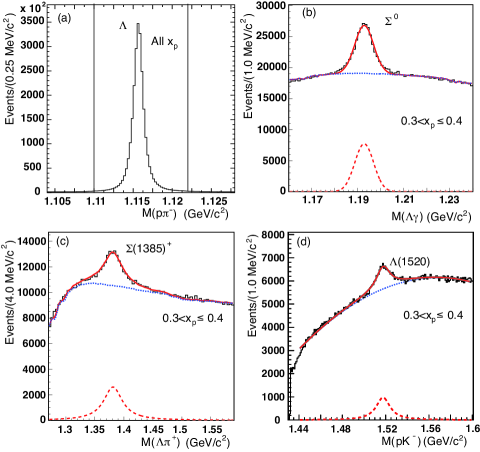
Figure 1: (a) The invariant-mass spectrum of ($p,\pi^{-}$). The vertical lines demarcate the signal region for $\Lambda$. (b), (c), (d) Invariant-mass spectra of ($\Lambda,\gamma$), ($\Lambda,\pi^{+}$), ($pK^{-}$), respectively. Fit results, signal shapes, and background shapes are shown by solid, dashed, and dotted curves, respectively.

We start with the analysis of the $\Lambda$ baryon. We reconstruct a $\Lambda\rightarrow p\pi^{-}$ decay candidate from a proton and a pion candidate, and obtain the decay point and the momentum of the $\Lambda$. The beam profile at the IP is wide in the horizontal direction ($x$) and narrow in vertical ($y$); the size of the IP region is typically $\sigma_{x}\sim 100$ $\mu$m, $\sigma_{y}\sim 5$ $\mu$m, and $\sigma_{z}\sim 3$ mm Belle_Vtx_resol . To select $\Lambda$ baryons that originate from the IP, we project the $\Lambda$ trajectory from its decay vertex toward the IP profile and then measure the difference along the $x$ direction between its production point and the IP centroid, $\Delta x$; we select events with $|\Delta x|<0.2$ cm. The $\Lambda$ candidates must have a flight length of 0.11 cm or more. The invariant-mass spectrum of the surviving $p\pi^{-}$ combinations is shown in Fig. 1(a). We can see an almost background-free $\Lambda$ peak. The events in the mass range of 1.110 GeV/$c^{2}$ $<M_{\Lambda}<1.122$ GeV/$c^{2}$ are retained. We investigate background events in the sideband regions of 1.104 GeV/$c^{2}$$<M_{\Lambda}<1.110$ GeV/$c^{2}$ and 1.122 GeV/$c^{2}$$<M_{\Lambda}<1.128$ GeV/$c^{2}$. Due to the detector resolution, some signal events spill out of the mass range. This signal leakage is estimated using Monte Carlo (MC) events, and is found to be about 4% and 1% of the events in the signal regions of $M_{\Lambda}$ and $\Delta x$, respectively. The MC study also shows that background events distribute rather evenly both in the invariant mass and $\Delta x$. Therefore, the background contributions are estimated by the sum of sideband events after subtracting the signal leakage.

Next, a $\Lambda$ candidate is combined with a photon or a $\pi^{+}$ to form a $\Sigma^{0}$ or a $\Sigma(1385)^{+}$ candidate, respectively. The energy of the photon from the $\Sigma^{0}$ decay must exceed 45 MeV to suppress backgrounds. The invariant-mass spectra of the $\Lambda\gamma$ and $\Lambda\pi^{+}$ combinations are shown in Figs. 1(b) and 1(c), where peaks of $\Sigma^{0}$ and $\Sigma(1385)^{+}$ are observed. Background shapes ($h(m)$) for $\Sigma^{0}$ and $\Sigma(1385)$ as functions of the invariant mass ($m$) are obtained using MC events of $e^{+}e^{-}\rightarrow q\bar{q}$ production, where $q=u,d,s,c$. We apply Wiener filter NumericalRevipes for $h(m)$ to avoid fluctuation due to the finite statistics of MC samples. For the fit the MC spectra to the real data, we multiply the first order polynomial function ($am+b$) to $h(m)$, where $a$ and $b$ are free parameters. The signal yields of $\Sigma^{0}$ are estimated by fitting the $\Lambda\gamma$ spectrum in the range 1.17 GeV/$c^{2}$$<M_{\Lambda\gamma}<$1.22 GeV/$c^{2}$ with a Gaussian and the background spectrum, where all parameters are determined from the fit. In this analysis, all fit parameters are floated in each $x_{p}$ bin unless otherwise specified. Note that the mass resolution for the signal is almost entirely determined by the energy resolution of the low-energy photon and can be approximated by a Gaussian shape. On the other hand, a non-relativistic Breit-Wigner function is used to estimate the signal yields of $\Sigma(1385)^{+}$ since the detector resolution is negligible compared to the natural width. The fit region is 1.3 GeV/$c^{2}$$<M_{\Lambda\pi^{+}}<$1.5 GeV/$c^{2}$, and all parameters are floated in the fit.

For the reconstruction of $\Lambda(1520)\rightarrow K^{-}p$, tracks identified as a kaon and a proton, each with a small impact parameter with respect to the IP, are selected. The invariant-mass spectrum of $K^{-}p$ pairs is shown in Fig. 1(d). A clear peak of the $\Lambda(1520)$ is seen above the combinatorial background. We employ a third-order polynomial for the background and a non-relativistic Breit-Wigner function to estimate the signal yields, where all parameters are floated except for the width of the Breit-Wigner function, which is fixed to the PDG value to stabilize the fit. The fit region is 1.44 GeV/$c^{2}<M_{K^{-}p}<1.6$ GeV/$c^{2}$.

II.2 $S=-2,-3$ hyperons

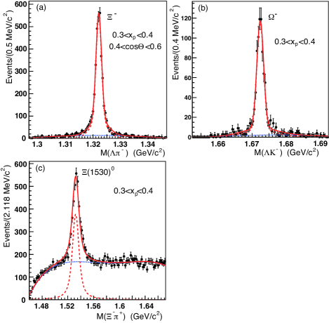
Figure 2: (a)-(c) Reconstructed mass spectra for $S=-2$ and $-3$ hyperon candidates. Fit results, signal shapes, and background shapes are shown by solid, dashed, and dotted curves, respectively.

The $\Xi^{-}$ and $\Omega^{-}$ are reconstructed from $\Xi^{-}\rightarrow\Lambda\pi^{-}$ and $\Omega^{-}\rightarrow\Lambda K^{-}$ decay modes, respectively. We reconstruct the vertex point of a $\Lambda\rightarrow p\pi^{-}$ candidate, as before, but do not impose the IP constraint on $\Delta x$ here to account for the long lifetime of the $S=-2,-3$ hyperons. Instead, the trajectory of the $\Lambda$ is combined with a $\pi^{-}$ ($K^{-}$) and the helix trajectory of the $\Xi^{-}$ ($\Omega^{-}$) candidate is reconstructed. This helix is extrapolated back toward the IP. The distance of the generation point of the $\Xi^{-}$ ($\Omega^{-}$) from IP along the radial ($dr$) and the beam direction ($dz$) must satisfy $dr<0.1$ (0.07) cm and $|dz|<2.0$ (1.1) cm. The invariant-mass spectra of $\Lambda\pi^{-}$ and $\Lambda K^{-}$ pairs are shown in Figs. 2(a) and 2(b). We see prominent peaks of $\Xi^{-}$ and $\Omega^{-}$. The $\Xi(1530)^{0}$ hyperon candidates are reconstructed from $\Xi^{-}\pi^{+}$ pairs, whose invariant mass is shown in Fig. 2(c).

Signal peaks of $\Xi^{-}$ and $\Omega^{-}$ are fitted with double-Gaussian functions, and those of $\Xi(1530)^{0}$ are fitted with Voigt functions. A second-order Chebyshev polynomial is used to describe background contributions. All parameters are floated. The fit regions are 1.28 GeV/$c^{2}<M_{\Lambda\pi^{-}}<1.375$ GeV/$c^{2}$, 1.465 GeV/$c^{2}<M_{\Xi^{-}\pi^{+}}<1.672$ GeV/$c^{2}$, and 1.652 GeV/$c^{2}<M_{\Lambda K^{-}}<1.692$ GeV/$c^{2}$ for $\Xi^{-}$, $\Xi(1530)^{0}$, and $\Omega^{-}$, respectively. The widths of $\Xi(1530)^{0}$ obtained by the fit are consistent with the PDG value.

II.3 Charmed baryons

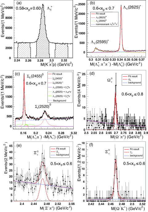
Figure 3: Reconstructed mass spectra of charmed baryon candidates. (a) The invariant-mass spectrum of $\Lambda_{c}^{+}$. The signal and sideband regions are indicated by the double-hatched and hatched histograms, respectively. (b) The mass-difference distribution of $\Lambda_{c}^{+}\pi^{+}\pi^{-}-\Lambda_{c}^{+}$. (c) The mass-difference distribution for $\Lambda_{c}^{+}\pi^{-}$-$\Lambda_{c}^{+}$. (d) The invariant-mass spectrum of $\Omega^{-}\pi^{+}$. (e), (f) The invariant-mass spectra of $\Xi^{-}\pi^{+}$ and $\Omega^{-}K^{+}$, respectively.

For the study of charmed baryons, we use both off- and on-resonance data, the latter recorded at the $\Upsilon(4S)$ energy ($\sqrt{s}=10.58$ GeV). To eliminate the $B$-meson decay contribution, the charmed-baryon candidates are required to have $x_{p}>0.44$ in the on-resonance data. For the reconstruction of charmed baryons, we apply the same PID and impact parameter criteria as for hyperons.

First, we reconstruct the $\Lambda_{c}^{+}$ baryon in the $\Lambda_{c}^{+}\rightarrow\pi^{+}K^{-}p$ decay mode. To improve the momentum resolution, we apply a vertex-constrained fit that incorporates the IP profile. We fit the invariant-mass spectra in 50 $x_{p}$ bins (Fig. 3(a)), and obtain peak positions and widths of $\Lambda_{c}^{+}$ as a function of the momentum (Fig. 4). The peak positions are slightly smaller than the PDG value by 1$\sim$1.4 MeV/$c^{2}$. In order to avoid misestimation of the yields, we select $\Lambda_{c}^{+}$ candidates whose mass ($M$) is within $3\sigma$ of the peak of a Gaussian fit ($M_{\Lambda_{c}}(x_{p})$) as signal. Candidates with $-11\sigma<|M-M_{\Lambda_{c}}(x_{p})-3~{}{\rm MeV}/c^{2}|<-5\sigma$ and $+5\sigma<|M-M_{\Lambda_{c}}(x_{p})+3~{}{\rm MeV}/c^{2}|<11\sigma$ are treated as sideband. We estimate background yields under the signal peak from the yields in the sidebands, and correct for reconstruction efficiency using MC $e^{+}e^{-}\rightarrow c\bar{c}$ events. In the $\Lambda_{c}^{+}\rightarrow\pi^{+}K^{-}p$ decay, the intermediate resonances ($K(890)^{0}$, $\Delta$, and $\Lambda(1520)$) can contribute, and the distribution in the Dalitz plane is not uniform Belle_Lc_double_cabbibo . To avoid the uncertainty in the reconstruction efficiency correction due to these intermediate states, the correction is applied for the Dalitz distribution of $\Lambda_{c}^{+}$ signal region after subtracting the sideband events. In the low $x_{p}$ region ($x_{p}\leq 0.44$), we obtain the cross section using off-resonance data, whereas we utilize both off- and on- resonance data in the high $x_{p}$ region ($x_{p}>0.44$).

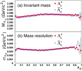
Figure 4: Invariant mass (a) and R.M.S. width (b) of the fitted $\Lambda_{c}^{+}$ and $\bar{\Lambda}_{c}^{-}$ as a function of $x_{p}$.

We reconstruct $\Sigma_{c}^{(*)0}$ or excited $\Lambda_{c}^{*+}$ states by combining a $\Lambda_{c}^{+}$ candidate with a $\pi^{-}$ or a $\pi^{+}\pi^{-}$ pair, respectively. Among several $\Lambda_{c}^{+}\pi^{-}$ ($\Lambda_{c}^{+}\pi^{+}\pi^{-}$) combinations in one event, we select the one with the best fit quality in the vertex-constraint fit. The background events are subtracted using the sideband distribution, as described above. Reconstructed invariant-mass spectra of $\Delta M(\pi\pi)={M}(\Lambda_{c}^{+}\pi^{+}\pi^{-})-{M}(\Lambda_{c}^{+})$ and $\Delta M(\pi^{-})={M}(\Lambda_{c}^{+}\pi^{-})-{M}(\Lambda_{c}^{+})$ are shown in Figs. 3(b) and 3(c), respectively. We see clear peaks of $\Lambda_{c}(2595)^{+}$ and $\Lambda_{c}(2625)^{+}$ in Fig. 3(b) and of $\Sigma_{c}(2455)^{0}$ and $\Sigma_{c}(2520)^{0}$ in Fig. 3(c). Since the peaks of these states are not statistically significant in the low $x_{p}$ region of the off-resonance data, we obtain the cross section in the $x_{p}>0.4$ region and extrapolate to the entire $x_{p}$ region using the Lund fragmentation model. The fragmentation-model dependence introduces a systematic uncertainty that is estimated by the variation using other models. The yields of these charmed baryons are obtained from fits to invariant-mass distributions in the mass range 0.28 GeV/$c^{2}<\Delta M({\pi\pi})<0.38$ GeV/$c^{2}$ and 0.145 GeV/$c^{2}<\Delta M({\pi^{-}})<0.32$ GeV/$c^{2}$ for excited $\Lambda_{c}$ baryons and $\Sigma_{c}$ baryons, respectively.

In the $\Delta M(\pi\pi)$ spectra, the background shape can be described by the combination of $\Lambda_{c}^{+}$ with pions that are not associated with resonances. We generate inclusive $e^{+}e^{-}\to\Lambda_{c}^{+}X$ MC events, and use the invariant mass of $\Lambda_{c}^{+}\pi^{+}\pi^{-}$ combinations to describe the background spectra. We use a Voigtian Voigt function to describe the line-shape of $\Lambda_{c}(2625)^{+}$, where the width and the resolution are set as free parameters. The widths obtained by the fit are smaller than 1 MeV/$c^{2}$, and are consistent with the upper limit ($0.97$ MeV/c²) in the PDG. The mass of $\Lambda_{c}(2595)^{+}$ is very close to the mass threshold of $\Lambda_{c}^{+}\pi^{+}\pi^{-}$ and so the line shape is asymmetric. We use the theoretical model of Cho ChoPRD50 to describe the line-shape of $\Lambda_{c}(2595)^{+}$, with parameters obtained by CDF CDF_PRD84012003 . This model describes the width of the $\Lambda_{c}(2595)^{+}$ as a function of the mass, and produces a long tail in the high-mass region. To reduce the systematic uncertainty due to the tail contribution, we evaluate the yield of the $\Lambda_{c}(2595)^{+}$ in the $\Delta M(\pi\pi)<0.33$ GeV/$c^{2}$ region. The systematic uncertainty due to this selection is estimated by changing the $\Delta M(\pi\pi)$ region, and is included in the systematic due to the signal shape in Table 3.

We also use Voigtian functions to describe $\Sigma_{c}(2455)^{0}$ and $\Sigma_{c}(2520)^{0}$; the Belle measurements Belle_ScWidth of the masses and widths are used. The fit results are shown in Figs. 3(b) and 3(c). In Fig. 3(c), the background spectrum exhibits a non-uniform structure due to the feed-down contribution from $\Lambda_{c}(2595)^{+}$ and $\Lambda_{c}(2625)^{+}$. These resonances decay into $\Lambda_{c}^{+}\pi^{+}\pi^{-}$, $\Sigma_{c}^{++}\pi^{-}$ $\Sigma_{c}^{+}\pi^{0}$, and $\Sigma_{c}^{0}\pi^{+}$, where $\Lambda_{c}^{+}\pi^{+}\pi^{-}$ and $\Sigma_{c}^{++}\pi^{-}$ modes are considered background. Feed-down contributions from $\Lambda_{c}^{+}$ excited states to the $\Sigma_{c}^{0}\pi^{+}$ mode is subtracted later. In the $\Delta M(\pi^{-})$ spectra of the $\Lambda_{c}^{*}\rightarrow\Lambda_{c}^{+}\pi^{+}\pi^{-}$, $\Sigma_{c}^{++}\pi^{-}$ reactions from MC simulation, a small enhancement around $\Delta M(\pi^{-})=0.187$ GeV/$c^{2}$ is likely due to the contribution from $\Xi_{c}^{0}$ as discussed in Ref. Belle_ScWidth , and a Gaussian function is used to describe this peak. The magnitude of background contributions is treated as a free parameter, and a fit including the signal peaks is shown in Fig. 3(c). The $\chi^{2}$ per the number of degrees of freedom ($ndf$) values are in the range from 148/163 to 203/163, and are reasonably good in each $x_{p}$ bin; deviations from the fit function are within statistical uncertainties.

Figure 3(d) shows the invariant-mass spectrum of $\Omega^{-}\pi^{+}$ pairs, where a peak corresponding to $\Omega_{c}^{0}$ is seen. The yields of $\Omega_{c}^{0}$ are obtained from fits to invariant-mass distributions in the range of 2.5 GeV/$c^{2}<M_{\Omega_{c}^{0}}<2.9$ GeV/$c^{2}$. The signal and background shapes are described by Gaussian functions and second-order Chebyshev polynomial functions, where the mean and width of Gaussian functions are allowed to float. $\Xi_{c}^{0}$ baryons are reconstructed in two decay modes: $\Xi_{c}^{0}\rightarrow\Xi^{-}\pi^{+}$ and $\Xi_{c}^{0}\rightarrow\Omega^{-}K^{+}$, as shown in Figs. 3(e) and 3(f). The yields of $\Xi_{c}^{0}$ are obtained from fits to invariant-mass distributions in the range of 2.321 GeV/$c^{2}<M_{\Xi_{c}^{0}}<2.621$ GeV/$c^{2}$. The signal and background shapes are described by double-Gaussian functions and second-order Chebyshev polynomial functions.

II.4 Inclusive cross sections

Table 1: Total cross sections before (visible) and after the radiative correction, where the first and second errors are statistical and systematic uncertainties. For the charmed strange baryons, the cross sections times branching fractions are listed.

Particle	Mode	Branching	Visible	Radiative corrected	Ratio of
		fraction	cross	cross	before and after
		(%)	section (pb)	section (pb)	the correction
$\Lambda$	$p\pi^{-}$	$63.9\pm 0.5$	$308.80\pm 0.37\pm 17$	$276.50\pm 0.33\pm 16$	0.895
$\Lambda(1520)$	$pK^{-}$	$22.5\pm 0.5$	$14.32\pm 0.23\pm 1.0$	$12.80\pm 0.20\pm 0.94$	0.894
$\Sigma^{0}$	$\Lambda\gamma$	$100$	$70.40\pm 0.73\pm 3.7$	$67.12\pm 0.69\pm 3.7$	0.953
$\Sigma(1385)^{+}$	$\Lambda\pi^{+}$	$87\pm 1.5$	$24.64\pm 0.39\pm 2.7$	$22.97\pm 0.32\pm 2.6$	0.932
$\Xi^{-}$	$\Lambda\pi^{-}$	$100$	$18.08\pm 0.18\pm 0.85$	$16.18\pm 0.16\pm 0.84$	0.895
$\Xi(1530)^{0}$	$\Xi^{-}\pi^{+}$	$50$	$4.32\pm 0.070\pm 0.21$	$3.855\pm 0.062\pm 0.20$	0.892
$\Omega^{-}$	$\Lambda\,K^{-}$	$67.8\pm 0.7$	$0.995\pm 0.019\pm 0.048$	$0.887\pm 0.017\pm 0.047$	0.891
$\Lambda_{c}^{+}$	$\pi^{+}K^{-}p$	$6.35\pm 0.33$	$157.76\pm 0.90\pm 8.0$	$141.79\pm 0.81\pm 7.8$	0.899
$\Lambda_{c}(2595)^{+}$	$\Lambda_{c}^{+}\pi^{+}\pi^{-}$	$34.6\pm 1.2$	$10.31\pm 0.011\pm 0.91$	$10.157\pm 0.011\pm 0.92$	0.985
$\Lambda_{c}(2625)^{+}$	$\Lambda_{c}^{+}\pi^{+}\pi^{-}$	$55.5\pm 1.1$	$15.86\pm 0.12\pm 1.3$	$15.37\pm 0.12\pm 1.3$	0.969
$\Sigma_{c}(2455)^{0}$	$\Lambda_{c}^{+}\pi^{-}$	$100$	$8.419\pm 0.073\pm 1.2$	$7.963\pm 0.069\pm 1.1$	0.946
$\Sigma_{c}(2520)^{0}$	$\Lambda_{c}^{+}\pi^{-}$	$100$	$8.31\pm 0.12\pm 1.3$	$7.77\pm 0.11\pm 1.3$	0.935
$\Omega_{c}^{0}$	$\Omega^{-}\pi^{+}$		$0.0153\pm 0.0020\pm 0.00070$	$0.0130\pm 0.0016\pm 0.00060$	0.850
$\Xi_{c}^{0}$	$\Xi^{-}\pi^{+}$		$0.376\pm 0.011\pm 0.013$	$0.332\pm 0.010\pm 0.013$	0.880
$\Xi_{c}^{0}$	$\Omega^{-}K^{+}$		$0.110\pm 0.052\pm 0.0038$	$0.097\pm 0.046\pm 0.0039$	0.880

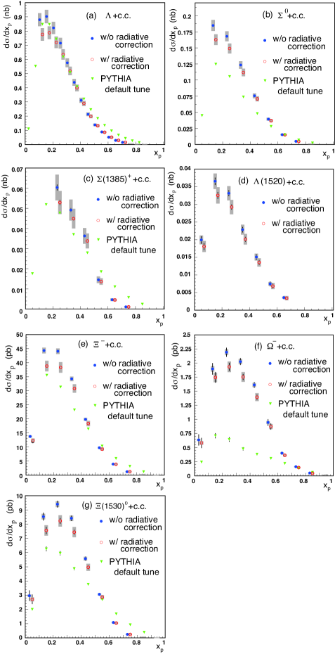
Figure 5: Differential inclusive cross sections of hyperons with and without radiative corrections. The closed circles are shifted slightly to the left for clarity. The error bars and shaded boxes represent the statistical and systematic uncertainties, respectively. These distributions contain feed-down contributions from heavier particles. Triangle points show predictions by PYTHIA with the default tune, where all radiative processes are turned off, and the feed-down contributions are obtained using PYTHIA predictions and branching fractions given in Ref. PDG2016 .

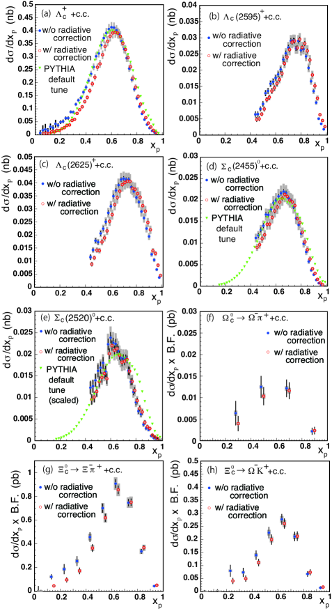
Figure 6: Differential inclusive cross sections of charmed baryon production with and without radiative corrections. The closed circles are shifted slightly to the left for clarity. The error bars and shaded boxes represent the statistical and systematic uncertainties, respectively. These distributions contain feed-down contributions from heavier particles. Triangle points show predictions by PYTHIA with the default tune, where all radiative processes are turned off, and the feed-down contributions are obtained using PYTHIA predictions and branching fractions given in Ref. PDG2016 . Note that the prediction for $\Sigma_{c}(2520)^{0}$ is scaled by a factor of $0.5$.

The yields of hyperons and charmed baryons are obtained as a function of the scaled momentum, and corrections for reconstruction efficiencies are applied in each $x_{p}$ bin. Reconstruction efficiencies are obtained using $e^{+}e^{-}\rightarrow q\bar{q}$ simulated events that contain the particle of interest in the final state. Since we apply the reconstruction efficiency correction in each $x_{p}$ bin, the potential discrepancy of the momentum distributions between MC and real data is avoided. The angular distributions of MC events are found to be consistent with those of real data. The reconstruction efficiencies used in this analysis are shown in Appendix A. The absolute branching fractions are obtained from Ref. PDG2016 and are used to calculate the production cross sections. The values used in this analysis are listed in Table 1. The differential cross sections are shown in Figs. 5 and 6. We note that these cross sections contain feed-down contributions from higher resonances (inclusive cross sections).

The correction factor due to the initial state radiation (ISR) and the vacuum polarization of the virtual gauge bosons in $e^{+}e^{-}$ annihilation is studied by PYTHIA PYTHIA by comparison between the cross sections computed with and without inclusion of the ISR and the vacuum polarization. Both virtual gamma and $Z^{0}$ exchanges including the interference between them are taken into account as the PYTHIA default. The effect of the final state radiation (FSR) from charged particles is investigated using PHOTOS program PHOTOS and we confirm that the FSR gives only negligible effect to present cross sections. For each particle species, MC events are generated with and without the ISR and the vacuum polarization effects and consequently $d\sigma/dx_{p}$ distributions are obtained. Using PYTHIA, the total hadronic cross sections with and without inclusion of the ISR and the vacuum polarization are calculated to be 3.3 nb and 2.96 nb respectively. We get the correction factors in each $x_{p}$ bin by taking the ratio between $d\sigma/dx_{p}$ for with and without radiative correction terms by scaling the ratio according to the calculated total hadronic cross sections. In the case of an ISR event the CM energy of the $e^{+}e^{-}$ annihilation process reduces and the true and reconstructed $x_{p}$ will be different. The ratio of $x_{p}$ distributions without ISR over ISR is taken to correct the differential cross sections. The differential cross sections before and after the correction are shown in Figs. 5 and 6.

Figures 5(a)-(d) show the differential cross sections for $S=-1$ hyperons. In the low $x_{p}$ and high $x_{p}$ regions, the signals of hyperons are not significant due to the small production cross sections and large number of background events. We obtain total cross sections over the entire $x_{p}$ region by utilizing a third-order Hermite interpolation describing the behavior in the measured $x_{p}$ range, where we assumed that the cross section is zero at $x_{p}=0$ and $x_{p}=1$. We obtain total cross sections over the entire $x_{p}$ region by utilizing a third-order Hermite interpolation describing the behavior in the measured $x_{p}$ range, where we assumed that the cross section is zero at $x_{p}=0$ and $x_{p}=1$. The estimated contributions from the unmeasured $x_{p}$ regions are 19%, 15%, and 49% of the contributions from the measured regions for $\Lambda$, $\Sigma^{0}$, $\Sigma(1385)^{+}$, and $\Lambda(1520)$, respectively. We also estimate the contributions from the unmeasured regions by assuming the PYTHIA spectrum shapes. The differences between the two estimations are typically 20-30% and assigned to the systematic errors for the extrapolation of the cross sections. For $S=-2$ and $-3$ hyperons, the cross sections are measured in the entire $x_{p}$ region.

The differential cross sections for charmed baryons after the correction for the reconstruction efficiency and the branching fractions are shown in Fig. 6. Here, we utilize the world-average absolute branching fraction of ${\cal B}(\Lambda_{c}^{+}\rightarrow K^{-}\pi^{+}p)=(6.35\pm 0.33)$% PDG2016 . The branching fractions of $\Lambda_{c}(2595)^{+}\rightarrow\Lambda_{c}^{+}\pi^{+}\pi^{-}$ and $\Lambda_{c}(2625)^{+}\rightarrow\Lambda_{c}^{+}\pi^{+}\pi^{-}$ are determined to be $0.346\pm 0.012\ ({\rm syst.})$ and $0.555\pm 0.011\ {\rm(syst.)}$, utilizing the model by Cho ChoPRD50 and accounting for the mass difference of the charged and neutral pion. Details are described in Appendix B. Since the absolute branching fractions of $\Omega_{c}^{0}\rightarrow\Omega^{-}\pi^{+}$, $\Xi_{c}^{0}\rightarrow\Xi^{-}\pi^{+}$ and $\Xi_{c}^{0}\rightarrow\Omega^{-}K^{+}$ are unknown, the cross section times the branching fraction are plotted in Figs. 6(f)-(h). The cross sections for $\Lambda_{c}(2595)^{+}$, $\Lambda_{c}(2625)^{+}$, $\Sigma_{c}(2455)^{0}$, and $\Sigma_{c}(2520)^{0}$ in the $0.44<x_{p}<1$ region after the radiative correction are $(9.60\pm 0.08)$ pb, $(11.39\pm 0.07)$ pb, $(6.34\pm 0.04)$ pb, and $(6.07\pm 0.08)$ pb, respectively. Clearly, the production cross sections for $\Lambda_{c}^{+}$ excited states are significantly higher than those for $\Sigma_{c}^{0}$ baryons in the measured $x_{p}$ region without the extrapolation to the whole $x_{p}$ region. We note that the radiative correction factors are consistent within 4% for these particles and are not the source of the difference of the production cross sections. We obtain cross sections of excited $\Lambda_{c}^{+}$ and $\Sigma_{c}^{0}$ states in the entire $x_{p}$ region utilizing the $x_{p}$ dependence of cross sections obtained from MC using the Lund model Andersson_PhysRept . The correction factors for extrapolating from the measured $x_{p}$ region to the entire $x_{p}$ region are small: 1.07, 1.07, 1.16, and 1.18 for $\Lambda_{c}(2595)$, $\Lambda_{c}(2625)$, $\Sigma_{c}(2455)^{0}$, and $\Sigma_{c}(2520)^{0}$, respectively. We obtain alternate correction factors using fragmentation models—BCFY BCFY , Bowler Bowler , Peterson Peterson , and KLP-B KLPB —and take the deviations of about 5 to 12% as the systematic uncertainty.

Table 1 shows cross sections before and after the radiative corrections. The correction factors are consistent for hyperons; however, larger correction factors by about 5% are obtained for the excited $\Lambda_{c}^{+}$ baryons than for $\Sigma_{c}^{0}$ baryons. The $d\sigma/dx_{p}$ distribution is harder for the excited $\Lambda_{c}^{+}$ baryons, as shown in Fig. 6, and the cross sections in the high-$x_{p}$ (low-$x_{p}$) region are increased (reduced) due to the radiative cross sections. As a result, we have larger correction factors for the excited $\Lambda_{c}^{+}$ baryons. The systematic uncertainties are discussed in Sec. II.5.

Triangle points in Figs. 5 and 6 show predictions by PYTHIA with default parameters, where all radiative processes are turned off. The feed-down contributions are obtained using PYTHIA predictions and branching fractions given in Ref. PDG2016 . Note that the prediction for $\Sigma_{c}(2520)^{0}$ overestimates the experimental data, and we scaled the predicted values by a factor of $0.5$.

II.5 Systematic uncertainties

Table 2: Systematic uncertainties (%) for the total cross section of hyperons and charmed strange baryons. The $\Lambda$ detection efficiency includes proton and pion identification efficiencies. The symbols of “-” and $\bigcirc$ mean that the uncertainty is much smaller than the statistical fluctuation and that the uncertainty is not taken into account, respectively.

Source	$\Lambda$	$\Sigma^{0}$	$\Sigma(1385)^{+}$	$\Lambda(1520)$	$\Xi^{-}$	$\Omega^{-}$	$\Xi(1530)^{0}$	$\Xi_{c}^{0}$ in	$\Xi_{c}^{0}$ in	$\Omega_{c}^{0}$
								$\Xi^{-}\pi^{+}$	$\Omega^{-}K^{+}$
Track reconstruction	0.70	0.70	1.1	0.70	1.1	1.1	1.4	1.4	1.4	1.4
$\Lambda$ detection	2.8	2.8	2.8	$\bigcirc$	3.3	3.2	3.0	3.3	3.2	3.2
$\gamma$ detection	$\bigcirc$	2.0	$\bigcirc$	$\bigcirc$	$\bigcirc$	$\bigcirc$	$\bigcirc$	$\bigcirc$	$\bigcirc$	$\bigcirc$
Particle ID	$\bigcirc$	$\bigcirc$	1.3	1.1	1.1	1.1	1.5	1.4	1.1	1.1
MC statistics	0.10	0.75	2.0	1.2	0.10	0.95	0.39	0.22	0.39	0.55
Signal shape	$\bigcirc$	1.4	0.57	2.8	0.2	0.6	2.0	3.4	0.2	1.2
Background estimation	$\bigcirc$	-	2.2	5.4	1.0	1.0	1.0	1.0	1.0	1.0
Experimental period	-	-	-	-	-	-	-	-	-	-
Baryon anti-baryon	-	-	-	-	-	-	-	-	-	-
Impact parameter	-	-	-	-	-	-	-	-	-	-
Extrapolation of $d\sigma/dx_{p}$	3.8	2.1	9.4	0.96	-	-	-	-	-	-
Radiative correction	2.3	2.3	2.3	2.3	2.3	2.3	2.3	2.3	2.3	2.3
Luminosity measurement	1.4	1.4	1.4	1.4	1.4	1.4	1.4	1.4	1.4	1.4
Total	5.5	5.1	11	6.9	4.6	4.7	5.0	5.8	4.7	4.7

Table 3: Systematic uncertainties (%) for the total cross section of charmed baryons. The symbols of “-” and $\bigcirc$ mean that the uncertainty is much smaller than the statistical fluctuation and that the uncertainty is not taken into account, respectively.

Source	$\Lambda_{c}^{+}$	$\Lambda_{c}(2595)^{+}$	$\Lambda_{c}(2625)^{+}$	$\Sigma_{c}^{0}$	$\Sigma_{c}(2520)^{0}$
Track reconstruction	1.1	1.8	1.8	1.4	1.4
Particle ID	2.0	3.9	4.0	5.0	1.4
MC statistics	0.27	0.10	0.30	0.10	0.14
Signal shape	$\bigcirc$	2.8	1.3	2.2	1.5
Background estimation	$\bigcirc$	2.0	2.3	1.0	7.5
Experimental period	1.8	-	-	2.5	5.9
Baryon anti-baryon	1.5	-	-	-	-
Impact parameter	2.2	-	-	-	-
$B$-meson decay	-	3.7	2.6	3.3	0.6
Extrapolation of $d\sigma/dx_{p}$	-	5.7	5.6	11	12
Radiative correction	2.3	2.3	2.3	2.3	2.3
Luminosity measurement	1.4	1.4	1.4	1.4	1.4
Total	4.8	9.1	8.4	13	16

The sources of systematic uncertainties are summarized in Tables 2 and 3. The uncertainties due to the reconstruction efficiency of charged particles and the $\Lambda$ selection including particle identification (particle ID) are estimated by comparing the efficiencies in real data and MC. The systematic uncertainty of photon detection efficiency for $\Sigma^{0}\rightarrow\Lambda\gamma$ decay is estimated to be 2% from a radiative Bhabha sample. The uncertainties of the particle ID for kaons, pions, and protons are estimated by comparing the efficiencies in real data and MC, where $D^{0}\rightarrow K^{-}\pi^{+}$ events and $\Lambda\rightarrow p\pi^{-}$ events are used for kaon (pion) selection and proton selection, respectively. The uncertainties of the reconstruction efficiency due to the statistical fluctuation of the MC data are taken as systematic uncertainties.

The signal shapes for $\Sigma^{0}$, $\Xi^{-}$, $\Omega^{-}$, $\Xi_{c}$, and $\Omega_{c}$ are assumed as double Gaussian. First, we confirm that the background shape is stable by changing the signal shape. We compare the signal yield with the one obtained by subtracting the background contribution from the total number of events, and take the difference as the systematic uncertainty due to the background shape. For excited particles, we estimate the systematic uncertainty due to the signal shape by fixing the resolution parameter of Voigtian function to the value obtained by MC. The yields of the ground-state $\Lambda$ and $\Lambda_{c}$ are obtained by sideband subtraction, and the systematic uncertainties due to the signal shape are not taken into account.

The uncertainty due to the background estimation for hyperons and charmed strange baryons is determined by utilizing a higher order polynomial to describe the background contribution and then redetermining the signal yield. For the yield estimation of excited charmed baryons, the background shape described by the threshold function is compared with the background shape obtained by MC, in which the threshold function is given by $a(m-m_{0})^{b}\exp(c(m-m_{0}))$, where $m$ is the invariant mass, $m_{0}$ is the threshold value, and $a$, $b$ and $c$ are fit parameters. The differences of the obtained signal yields are taken as the systematic uncertainty. The yields of the $\Lambda$ and $\Lambda_{c}^{+}$ baryons are obtained by sideband subtraction. Because the uncertainty of the background estimation is included in the statistical uncertainties here, this uncertainty is not taken as a systematic uncertainty.

To evaluate other sources of systematic uncertainties, the cross sections are compared using subsets of the data: events recorded in the different experimental periods, or the baryon vs. anti-baryon samples. In addition, the cross sections are compared by changing the event-selection criteria: impact-parameter requirements for tracks, or the $x_{p}$ threshold to eliminate the $B$-meson decay contribution for excited $\Lambda_{c}$ and $\Sigma_{c}$ baryons. If these differences are larger than the statistical fluctuation, we take them as systematic uncertainties.

We estimate the uncertainties due to the extrapolation to the whole $x_{p}$ range for $S=-1$ hyperons using, the $d\sigma/dx_{p}$ distribution of MC events for the extrapolation, which are generated using Lund fragmentation model. We compare the results of the extrapolation using all measured points and only the lowest $x_{p}$ data (where the feed-down contribution is large); and the largest discrepancy is taken as the systematic uncertainty.

The systematic uncertainty due to the radiative correction is estimated using PYTHIA. However, because we apply radiative corrections in each $x_{p}$ bin, we expect the dependence of the correction factors on the fragmentation model to be reduced. The largest difference of the correction factors for different PYTHIA tunes, which were described in Ref. Belle_pair_cross_section , is 2.1%, and is taken as a systematic uncertainty that is common for all $x_{p}$ bins. An additional uncertainty due to the accuracy of radiative effects in the generator is estimated to be 1% Kleiss_Z_LEP , and is taken as a systematic uncertainty.

The uncertainty due to the luminosity measurement (1.4%) is common for all particles. The $x_{p}$ dependence of the systematic uncertainty is found to be less than 0.4% and is negligible for all particles.

II.6 Direct cross sections

Table 4: Direct cross sections after the feed-down subtraction, and the fraction of the direct cross sections with respect to the radiative-corrected cross sections. Direct cross sections predicted by PYTHIA with default parameters are listed for the positive-parity baryons, where radiative processes are turned off. The masses and spins used in Figs. 8 and 9 are itemized.

Particle	Mass	Spin	Direct	Fraction	PYTHIA
	(MeV/$c^{2}$)		cross		prediction
			section (pb)		(pb)
$\Lambda$	1115.6	1/2	$91.2\pm 2.1\pm 22$	0.32	$87.7\pm 0.4$
$\Lambda(1520)$	1519.5	3/2	$9.68\pm 0.75\pm 0.26$	0.73
$\Sigma^{0}$	1192.6	1/2	$52.28\pm 0.66\pm 3.8$	0.83	$36.1\pm 0.3$
$\Sigma(1385)^{+}$	1382.8	3/2	$18.39\pm 0.35\pm 2.8$	0.83	$19.8\pm 0.2$
$\Xi^{-}$	1321.4	1/2	$11.25\pm 0.17\pm 0.33$	0.7	$10.8\pm 0.1$
$\Xi(1530)^{0}$	1531.8	3/2	$3.855\pm 0.062\pm 0.22$	1.0	$2.58\pm 0.07$
$\Omega^{-}$	1672.4	1/2	$0.887\pm 0.017\pm 0.047$	1.0	$0.32\pm 0.02$
$\Lambda_{c}^{+}$	2286.4	1/2	$67.6\pm 1.5\pm 9.1$	0.48	$85.8\pm 0.3$
$\Lambda_{c}(2595)^{+}$	2592.2	1/2	$10.157\pm 0.011\pm 0.92$	1.0
$\Lambda_{c}(2625)^{+}$	2628.1	3/2	$15.367\pm 0.116\pm 1.3$	1.0
$\Sigma_{c}(2455)^{0}$	2453.7	1/2	$6.697\pm 0.069\pm 1.2$	0.84	$8.5\pm 0.1$
$\Sigma_{c}(2520)^{0}$	2518.8	3/2	$7.77\pm 0.11\pm 1.3$	1.0	$16.6\pm 0.1$

Our motivation is to search for the enhancement or the reduction of the production cross sections of certain baryons and to discuss their internal structures, as described in Sec. I. For this purpose, the subtraction of feed-down from heavier particles is quite important since the amount of this feed-down is determined by the production cross sections of mother particles and the branching fractions, which are not related to the internal structure of the baryon of interest. Table 4 shows the inclusive cross sections after the feed-down subtraction (direct cross section) and their fraction of the cross sections after the radiative correction. The branching fractions and feed-down contributions are summarized in Appendix B. We use the world-average branching fractions in Ref. PDG2016 . We should note that the cited list may be incomplete, i.e., we may have additional feed-down contributions. Such contributions are expected to be small, and should be subtracted when the branching fractions are measured in the future. While the calculation of the feed-down contributions, the same production rates are assumed for iso-spin partners ($\Sigma(1385)$, $\Xi$, $\Xi(1530)$, $\Sigma_{c}(2455)$, $\Sigma_{c}(2520)$). The branching fraction of ${\cal B}(\Lambda_{c}(2595)^{+}\rightarrow\Lambda_{c}^{+}\pi^{+}\pi^{-})$ is obtained to be $0.346\pm 0.012\ ({\rm syst.})$ using Cho’s function ChoPRD50 with the parameter obtained by CDF CDF_PRD84012003 . More details are described in Appendix B.

The systematic uncertainties for the feed-down contribution are calculated using those for the inclusive cross sections of mother particles, and we use the quadratic sum for the systematic uncertainty of the direct cross section. The uncertainty of the luminosity measurement is common to all baryons, and, in order to avoid double counting, we add the uncertainty due to the luminosity to the cross sections after the feed-down subtraction. The uncertainties for the branching fractions are taken as the systematic uncertainties for the direct cross sections.

III Results and discussion

III.1 Scaled momentum distributions

We discuss the differential cross sections first. The open circles in Figs. 5 and 6 show $d\sigma/dx_{p}$ for hyperons and charmed baryons after the radiative correction. The differential production cross sections of hyperons peak in the small $x_{p}$ region compared to those of charmed baryons. This behavior suggests that, at energies near $\sqrt{s}=10.5$ GeV, $s\bar{s}$ pairs that lead to hyperons are created mainly in the soft processes in the later stage of the fragmentation rather than in the hard processes of prompt $s\bar{s}$ creation from the initial virtual photon. The $d\sigma/dx_{p}$ distribution of charmed baryons show peaks in the high $x_{p}$ region, since $c\bar{c}$ pairs are created predominantly in the prompt $e^{+}e^{-}$ collision, and charmed baryons carry a large fraction of the initial beam energy.

The peak cross section of the hyperons occurs below $x_{p}=0.2$ and is consistent for all $S=-1$ hyperons. The $d\sigma/dx_{p}$ distributions for $S=-2,-3$ hyperons (Figs. 5(e)-(g)) exhibit peaks at slightly higher $x_{p}$ ($x_{p}>0.2$) than for $S=-1$ hyperons. Since the strange quark is heavier than the up or down quark, the energy necessary to create an $S=-2$ hyperon is larger than an $S=-1$ hyperon, and $S=-2$ hyperons may be produced in a rather harder process than $S=-1$ ones.

The distribution for the $\Lambda_{c}(2286)^{+}$ peaks at $x_{p}=0.64$, and that for the $\Sigma_{c}(2455)^{0}$ peaks at $x_{p}=0.68$. The peak position for the $\Sigma_{c}(2520)^{0}$ is not determined clearly due to the statistical fluctuations. The distributions for the $\Lambda_{c}(2595)^{+}$ and the $\Lambda_{c}(2625)^{+}$ show peak structures at significantly higher $x_{p}$ ($x_{p}=0.78$). The peak position for the $\Xi_{c}(2470)^{0}$ is around $x_{p}=0.65$, which is consistent with the $\Lambda_{c}(2286)^{+}$ and the $\Sigma_{c}(2455)^{0}$.

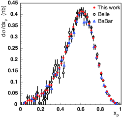
Figure 7: The differential cross sections of $\Lambda_{c}^{+}$ production before the radiative correction, where the absolute branching fraction of ${\cal B}(\Lambda_{c}^{+}\rightarrow\pi^{+}K^{-}p)=0.0635$ is used to normalize the previous results BaBar_Lc ; Belle_Charm_Seuster for the comparison. To scale the multiplicity measurement by BaBar, the total hadronic cross section of 3.3 nb is utilized. The error bars represent the sum in quadrature of the statistical and systematic uncertainties; note that Belle’s previous measurement contains an additional uncertainty of 35% for the normalization.

III.2 Comparison of inclusive cross sections with previous results

Table 5 shows a comparison with previous measurements, where for hyperons, we use the hadron multiplicities that were measured by ARGUS ARGUS_hyperon ; ARGUS_L1520 , since the statistics of other results are quite limited. For charmed baryons, we utilize the measurement of $\Lambda_{c}^{+}$ production by BaBar BaBar_Lc and the ratios of production rates of excited particles relative to the $\Lambda_{c}^{+}$ measured by CLEO CLEO_Lc2595_2625 ; CLEO_Sc2455 ; CLEO_Sc2520 and ARGUS ARGUS_Lc2595 ; ARGUS_Lc2625 . For the comparison, we utilize the world-average absolute branching fraction of ${\cal B}(\Lambda_{c}^{+}\rightarrow\pi^{+}K^{-}p)=0.0635$ PDG2016 to normalize the previous results of charmed baryons. Since previous measurements report cross sections without the radiative correction, we compare our results for the visible cross section. The total hadronic cross section of 3.3 nb CLEO_Hadronic is used to normalize hadron multiplicities to cross sections.

The differential cross section of $\Lambda_{c}^{+}$ production before the radiative correction is compared with the prior measurements by BaBar BaBar_Lc and BelleBelle_Charm_Seuster as shown in Fig. 7. For comparison, the absolute branching fraction of ${\cal B}(\Lambda_{c}^{+}\rightarrow\pi^{+}K^{-}p)=0.0635$ PDG2016 is used to rescale both of the BaBar and Belle measurements for this figure. To scale the multiplicity measurement by BaBar, the total hadronic cross section of 3.3 nb is utilized. Our result is consistent with these previous measurements.

We observe that the production cross sections of hyperons are consistent with previous measurements but with much higher precision. Here, it is noted that the statistics of the $\Lambda(1520)$ in the ARGUS result is quite limited. Their result is slightly larger than this work; however, is consistent within 2.0$\sigma$ due to the large uncertainty on their measurement. The production rate of the $\Lambda_{c}(2595)^{+}$ by this work is larger than the CLEO result; the corresponding ARGUS result ARGUS_Lc2595 is consistent with ours, but contains a large uncertainty due to the extrapolation to the whole $x_{p}$ region. ARGUS reported a more precise production cross section for $x_{p}>0.7$ of $(8.0\pm 2.3\,({\rm stat.})\pm 1.7\,({\rm syst.}))$ pb, which is consistent with our result of $(7.34\pm 0.06\ ({\rm stat.}))$ pb. The production rate of the $\Lambda_{c}(2625)^{+}$ in this work is significantly larger than the CLEO result. The ratio of production rates of the $\Lambda_{c}(2625)^{+}$ to the $\Lambda_{c}(2595)^{+}$ is about 1.3 and is consistent with this work. The result obtained by ARGUS is slightly larger than the CLEO result and closer to our result.

Table 5: Comparison of visible cross sections with previous measurements. The first and second errors represent the statistical and systematic uncertainties, respectively.

Particle	Visible cross section	Visible cross section by	References for
	by this work (pb)	previous measurements (pb)	previous measurements
$\Lambda$	$308.8\pm 0.37\pm 17$	$306\pm 10\pm 26$	ARGUS_hyperon
$\Lambda(1520)$	$14.32\pm 0.23\pm 1.0$	$26.6\pm 5.7\pm 4.3$	ARGUS_L1520
$\Sigma^{0}$	$70.40\pm 0.73\pm 3.7$	$76\pm 22\pm 16$	ARGUS_hyperon
$\Sigma(1385)^{+}$	$24.64\pm 0.39\pm 2.7$	$17.1\pm 3.1\pm 3.1$	ARGUS_hyperon
$\Xi^{-}$	$18.08\pm 0.18\pm 0.85$	$22\pm 2\pm 2$	ARGUS_hyperon
$\Xi(1530)^{0}$	$4.32\pm 0.070\pm 0.21$	$4.9\pm 1.7\pm 0.77$	ARGUS_hyperon
$\Omega^{-}$	$0.995\pm 0.019\pm 0.048$	$2.4\pm 1.2\pm 0.43$	ARGUS_hyperon
$\Lambda_{c}^{+}$	$157.76\pm 0.90\pm 8.0$	$148.9\pm 1.8\pm 1.6$	BaBar_Lc
$\Lambda_{c}(2595)^{+}$	$10.31\pm 0.011\pm 0.91$	$6.1\pm 1.0\pm 1.3$	CLEO_Lc2595_2625
$\Lambda_{c}(2595)^{+}$		$11.2^{+10.8}_{-5.8}\pm 8.3$	ARGUS_Lc2595
$\Lambda_{c}(2625)^{+}$	$15.86\pm 0.12\pm 1.3$	$7.80\pm 0.76\pm 0.62$	CLEO_Lc2595_2625
$\Lambda_{c}(2625)^{+}$		$10.8\pm 2.4\pm 2.8$	ARGUS_Lc2625
$\Sigma_{c}^{0}$	$8.419\pm 0.073\pm 1.2$	$8.9\pm 1.5\pm 2.5$	CLEO_Sc2455
$\Sigma_{c}(2520)^{0}$	$8.31\pm 0.12\pm 1.3$	$9.5\pm 1.1\pm 2.4$	CLEO_Sc2520

III.3 Mass dependence of direct production cross sections

We divide the direct production cross sections by the number of spin states $(2J+1)$ and plot these as a function of baryon masses (Figs. 8 and 9). The error bars represent the sum in quadrature of the statistical and systematic uncertainties. In Fig. 8, the production cross sections of $S=-1$ hyperons show an exponential dependence on the mass except for the $\Sigma(1385)^{+}$. We fit the production cross sections of $S=-1$ hyperons except for the $\Sigma(1385)^{+}$ using an exponential function,

$$f(m)=a_{0}\exp(a_{1}m),$$ (1)

where $m$ is the mass of the particle and $a_{0}$ and $a_{1}$ are fit parameters; we obtain $a_{0}=(1.6\pm 0.7)\times 10^{5}$ pb, $a_{1}=(-7.3\pm 0.3)/$(GeV/c²). Due to the large uncertainty on the $\Lambda$ hyperon, the $\chi^{2}/ndf$ value is very small.

We do not observe the enhancements of the direct cross sections of $\Lambda$ and $\Lambda(1520)$ that were discussed in Refs. Jaffe_Exotica ; Wilczek_diquark because they used data of inclusive production, which contain large feed-down contributions from heavier particles. The scaled direct cross sections for $\Lambda$, $\Sigma^{0}$ and $\Lambda(1520)$ follow an exponential mass dependence with a common slope parameter. The scaled direct cross section for $\Sigma(1385)^{+}$ is smaller than the predicted value of the exponential curve at $m=1.382$ GeV/c² by 30 % with the statistical significance of 2.8$\sigma$, as was reported by ARGUS ARGUS_hyperon . We found that the fit including the $\Sigma(1385)^{+}$ results in the deviation of 2.2$\sigma$. As already mentioned, the predicted production rate of the diquark model is smaller than that of the popcorn model by 30 %. However, these predictions include feed-down contributions, and predictions for the direct production cross sections are desired.

Since the mass of a strange quark is heavier than of an up or down quark, the probability of the $s\bar{s}$ pair creation is expected to be smaller than that of the non-strange quark pair creation. Indeed, $S=-2$ and $-3$ hyperons have significantly smaller production cross sections compared to $S=-1$ hyperons, which are likely due to the suppression of $s\bar{s}$ pair creation in the fragmentation process. Despite the mass difference between strange and lighter quarks, one may expect the same mechanism to form a baryon between $S=-1$ and $S=-2$ hyperons. The dashed line in Fig. 8 shows an exponential curve with the same slope parameter as $S=-1$ hyperons, which is normalized to the production cross section of $\Xi^{-}$. Clearly, the production cross section of the $\Xi(1530)^{0}$ is suppressed with respect to this curve. This may be due to the decuplet suppression noted in the $\Sigma(1385)^{+}$ case. The production cross section for the $S=-3$ hyperon, $\Omega^{-}$, shows further suppression for the creation of an additional strange quark.

The results for charmed baryons are shown in Fig. 9. The production cross section of the $\Sigma_{c}(2800)$ measured by Belle Belle_Sigmac2800 is shown in the same figure, where we utilize the weighted average of cross sections for the three charged states, and assume that the $\Lambda_{c}^{+}\pi$ decay mode dominates over the others. In Ref. Belle_Sigmac2800 , the spin-parity is tentatively assigned as $J^{P}=3/2^{-}$, so we use a spin of $3/2$ for this state.

The prompt production of a $q\bar{q}$ pair from $e^{+}e^{-}$ annihilation couples to the charge of quarks. If the center-of-mass energy of $e^{+}e^{-}$ is high compared to the mass of the charm quarks, the production rates of charm quarks become consistent with those of up quarks. Indeed, near the $\Upsilon(4S)$ energy, the production cross section of the $\Lambda_{c}^{+}$ ground state is much higher than the exponential curve of hyperons in Fig. 8 extended to the mass of charmed baryons. The production mechanism of charmed baryons differs from that of hyperons. For charmed baryons, a $c\bar{c}$ pair is created from the prompt $e^{+}e^{-}$ annihilation and picks up two light quarks to form a charmed baryon. Since this process occurs in the early stage of the fragmentation process where the number of quarks are few, the probability to form a charmed baryon from uncorrelated quarks is smaller than that from diquark and anti-diquark production. In addition to the production mechanism, we note that the diquark correlation in the charmed baryons are stronger than that in hyperons due to the heavy charm quark mass as discussed in Sec. I. Although these interpretations are model dependent, we can expect that the production cross sections of charmed baryons are related to the production cross sections of diquarks.

The production cross sections of $\Sigma_{c}$ baryons are smaller than those of excited $\Lambda_{c}^{+}$ by a factor of about three, in contrast to hyperons where $\Lambda$ and $\Sigma$ resonances lie on a common exponential curve. This suppression is already seen in the cross section in the $0.4<x_{p}<1$ region, and is not due simply to the extrapolation by the fragmentation models.

Table 4 shows the direct cross sections predicted by PYTHIA6.2 using default parameters. Note that PYTHIA can not produce negative-parity baryons. The predicted cross sections are consistent with the experimental measurements for hyperons except for $\Sigma^{0}$, $\Xi(1530)^{0}$ and $\Omega^{-}$. However, for charmed baryons, PYTHIA overestimate the experimental results. Since theoretical predictions for the production rates of charmed baryons are not available, we analyze our data assuming the diquark model and compare the obtained diquark masses those used for the hyperon production in Ref. Andersson_PhysRept . We fit the production cross sections of $\Lambda_{c}^{+}$ baryons and $\Sigma_{c}$ baryons using exponential functions, shown as the solid and dashed lines in Fig. 9. We obtain parameters of Eq. 1 to be $a_{0}=(6.2\pm 7.0)\times 10^{7}$ pb, $a_{1}=(-6.3\pm 0.5)/$(GeV/$c^{2}$) with $\chi^{2}/ndf=0.2/1$ for the $\Lambda_{c}^{+}$ family and $a_{0}=(4.6\pm 12.0)\times 10^{6}$ pb, $a_{1}=(-5.8\pm 1.0)/$(GeV/$c^{2}$) with $\chi^{2}/ndf=0.5/1$ for the $\Sigma_{c}$ family. The slope parameters for $\Lambda_{c}^{+}$ baryons and $\Sigma_{c}^{0}$ baryons are consistent within statistical uncertainties, and the ratio of production cross sections of $\Sigma_{c}^{0}$ to $\Lambda_{c}^{+}$ baryons is $0.27\pm 0.07$, using the weighted average of the slope parameters $\langle a_{1}\rangle=-6.2/$(GeV/$c^{2}$). Note that the uncertainties of the $a_{0}$ parameters are reduced by fixing the $a_{1}$ parameter. In the relativistic string fragmentation model Andersson_PhysRept , $q\bar{q}$ pairs are created in the strong color force in analogy with the Schwinger effect in QED. Similarly, in the diquark model, a diquark and anti-diquark pair is created to form a baryon or an anti-baryon. Assuming that the production cross sections of charmed baryons are proportional to the production probability of a diquark, the ratio of the production cross sections of $\Lambda_{c}^{+}$ resonances and $\Sigma_{c}$ resonances is proportional to $\exp(-\pi\mu^{2}/\kappa)$ Andersson_PhysicaScripta , where $\kappa$ is the string tension, $\kappa/\pi\sim 250^{2}$ (MeV²), and $\mu$ is the mass of the diquark. The obtained mass squared difference of spin-0 and 1 diquark, ${m}({ud}_{1})^{2}-{m}({ud}_{0})^{2}$, is $(8.2\pm 0.8)\times 10^{4}$ (MeV/$c^{2}$)². This is slightly higher than but consistent with the value described in Ref. Andersson_PhysRept , $490^{2}-420^{2}=6.4\times 10^{4}$ (MeV/$c^{2}$)². Our results favor the diquark model in the production mechanism of charmed baryons and a spin-0 diquark component of the $\Lambda_{c}^{+}$ ground state and low-lying excited states.

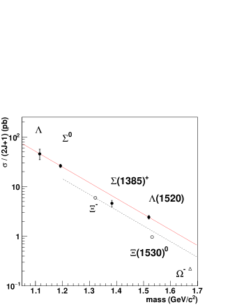
Figure 8: Scaled direct production cross section as a function of mass of hyperons. $S=-1,-2,-3$ hyperons are shown with filled circles, open circles and a triangle, respectively. The solid line shows the fit result using an exponential function (Eq.1) for $S=-1$ hyperons except for $\Sigma(1385)^{+}$. The dashed line shows an exponential curve with the same slope parameter as $S=-1$ hyperons, which is normalized to the production cross section of $\Xi^{-}$.

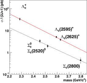
Figure 9: Scaled direct production cross section as a function of mass of charmed baryons. The solid and dashed lines show the fit results using exponential functions (Eq.1) for $\Lambda_{c}$ baryons and $\Sigma_{c}$ baryons, respectively.

IV Summary

We have measured the inclusive production cross sections of hyperons and charmed baryons from $e^{+}e^{-}$ annihilation near the $\Upsilon(4S)$ energy using high-statistics data recorded at Belle. The direct production cross section divided by the spin multiplicities for $S=-1$ hyperons except for $\Sigma(1385)^{+}$ lie on one common exponential function of mass. A suppression for $\Sigma(1385)^{+}$ and $S=-2,-3$ hyperons is observed, which is likely due to decuplet suppression and strangeness suppression in the fragmentation. The production cross sections of charmed baryons are significantly higher than those of excited hyperons, and strong suppression of $\Sigma_{c}$ with respect to $\Lambda_{c}^{+}$ is observed. The ratio of the production cross sections of $\Lambda_{c}^{+}$ and $\Sigma_{c}$ is consistent with the difference of the production probabilities of spin-0 and spin-1 diquarks in the fragmentation process. This observation supports the theory that the diquark production is the main process of charmed baryon production from $e^{+}e^{-}$ annihilation, and that the diquark structure exists in the ground state and low-lying excited states of $\Lambda_{c}^{+}$ baryons.

Appendix A Reconstruction efficiency

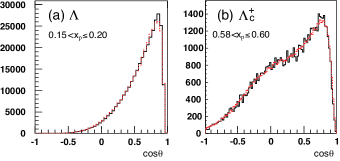
Figure 10: Polar angular distribution for $\Lambda$ (a) and $\Lambda_{c}^{+}$ (b) in the laboratory system. Solid (dotted) histograms show the distributions of real (MC) data.

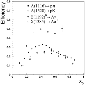
Figure 11: Reconstruction efficiencies for $S=-1$ hyperons.

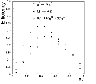
Figure 12: Reconstruction efficiencies for $S=-2,-3$ hyperons.

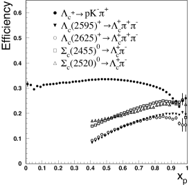
Figure 13: Reconstruction efficiencies for charmed baryons.

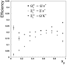
Figure 14: Reconstruction efficiencies for charmed strange baryons.

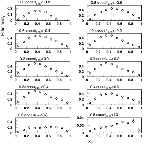
Figure 15: Reconstruction efficiencies for $\Xi^{-}$ hyperons in the $e^{+}e^{-}$ center of mass system.

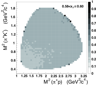
Figure 16: Reconstruction efficiency over the Dalitz plot for $\Lambda_{c}^{+}\rightarrow pK^{-}\pi^{+}$.

The reconstruction efficiencies are obtained using MC event samples that are generated using PYTHIA. The angular distributions of each particle are well reproduced by the MC event generator. Figure 10 shows the polar angular distribution of the $\Lambda$ and $\Lambda_{c}^{+}$ in the laboratory system for the real data and MC. The detector responses are simulated using GEANT3 package. In order to cancel the difference in the momentum distribution between real and MC events, the corrections for the reconstruction efficiencies are applied in each $x_{p}$ bin as shown in Figs. 11-14.

The trajectory of the $\Xi^{-}$ ($\Omega^{-}$) hyperon is reconstructed from the momentum and vertex point of a $\Lambda\pi^{-}$ ($\Lambda K^{-}$) pair, and the closest point with respect to the IP is obtained. Because the reconstruction of the momentum vector of these hyperons at the IP is complicated compared to $S=-1$ hyperons, the reconstruction efficiencies are obtained in each angular and $x_{p}$ bin. The correction factors for $\Xi^{-}$ are shown in Fig. 15 as an example.

In the $\Lambda_{c}^{+}\rightarrow\pi^{+}K^{-}p$ decay, the intermediate resonances ($K(890)^{0}$, $\Delta$, and $\Lambda(1520)$) can contribute as described in Sec. II.3. To avoid the uncertainty in the reconstruction efficiency correction due to these intermediate states, the correction is applied for the Dalitz distribution of $\Lambda_{c}^{+}$ signal region after subtracting the sideband events. Fig. 16 shows the reconstruction efficiency over the Dalitz plot for $\Lambda_{c}^{+}\rightarrow pK^{-}\pi^{+}$ in the region of $0.58<x_{p}<0.6$.

Appendix B feed-down from higher resonances

In order to obtain the direct production cross sections, the feed-down contributions from heavier states are subtracted. We consider all feed-down contributions that are listed in the PDG PDG2016 . There may be decay modes that have not yet been measured, and so are not listed. Thus, the “true” direct cross sections may be smaller. However, the production cross sections of heavy particles are expected to be suppressed according to the exponential mass dependence, and feed-down contributions from heavier particles should be small.

The feed-down contributions are summarized in Tables 6–11. Table 4 shows a summary of the inclusive and direct cross sections. We use the values of the inclusive cross sections that are obtained by this work. The branching fractions are obtained from Ref. PDG2016 .

A preliminary measurement of the branching fraction of inclusive $\Lambda_{c}^{+}\rightarrow\Lambda X$ decay is found to be $0.3698\pm 0.0218$ by BES III BES_Lc_Lambda . This inclusive branching fraction contains $\Lambda_{c}^{+}\rightarrow\Sigma^{0}X\rightarrow\Lambda\gamma X$ decay mode. In order to avoid double counting of feed-down from $\Sigma^{0}$, we need to eliminate the inclusive $\Lambda_{c}^{+}\rightarrow\Sigma^{0}X$ mode. However, this decay mode has not yet been measured. If we use exclusive decay modes, $\Lambda_{c}^{+}\rightarrow\Sigma^{0}\pi^{+}$ (1.29%), $\Lambda_{c}^{+}\rightarrow\Sigma^{0}\pi^{+}\pi^{0}$ (2.3%), $\Lambda_{c}^{+}\rightarrow\Sigma^{0}\pi^{+}\pi^{+}\pi^{-}$ (1.13%), $\Lambda_{c}^{+}\rightarrow\Lambda X$ becomes 32.26%. The amount of feed-down from $\Lambda_{c}^{+}$ to $\Lambda$ is estimated as $141.79\times 0.3226=45.74$ pb. The sum of the feed-down from $\Lambda_{c}^{+}$ listed in Table 6 is 32.17 pb. We take the difference of these two values, $45.74-32.17=13.57$ pb, as the systematic uncertainty for the feed-down from $\Lambda_{c}^{+}$ to $\Lambda$.

The branching fraction of ${\cal B}(\Lambda_{c}(2595)^{+}\rightarrow\Lambda_{c}^{+}\pi^{+}\pi^{-})$ is obtained to be $0.346\pm 0.012\ ({\rm syst.})$ using Cho’s function ChoPRD50 with the parameter obtained by CDF CDF_PRD84012003 . In this calculation, we integrate the mass spectrum of $\Lambda_{c}(2595)^{+}$ in the range of $0.28$ GeV/$c^{2}$$<\Delta M(\pi\pi)<0.33$ GeV/$c^{2}$, and estimate the uncertainty by changing the mass range with $\pm 5$ MeV, which is conservatively larger than the mass resolution. Taking into account the world-average relative branching fraction of ${\cal B}(\Sigma_{c}(2455)^{0}\pi^{+})/({\cal B}(\Sigma_{c}(2455)^{0}\pi^{+})+{\cal B}(\Sigma_{c}(2455)^{++}\pi^{-})+{\cal B}($non-resonant$\,\Lambda_{c}^{+}\pi^{+}\pi^{-}))=0.36\pm 0.10$, we obtain ${\cal B}(\Lambda_{c}(2595)^{+}\rightarrow\Sigma_{c}(2455)^{0}\pi^{+})=0.125\pm 0.034$.

Table 6: Feed-down to $\Lambda$. For the sum of the systematic uncertainties of the feed-down from $\Lambda_{c}^{+}$, the difference of the branching fractions of inclusive $\Lambda_{c}^{+}\rightarrow\Lambda X$ and exclusive decay modes is used as described in the text.

Decay mode	Branching	Feed-down (pb)
	fraction
$\Sigma(1192)^{0}\rightarrow\Lambda\gamma$	1	$63.44\pm 0.66\pm 3.2$
$\Sigma(1385)^{\pm,0}\rightarrow\Lambda\pi^{\pm,0}$	$0.87\pm 0.015$	$57.99\pm 0.92\pm 6.5$
$\Sigma(1385)^{0}\rightarrow\Lambda\gamma$	$0.0125\pm 0.0012$	$0.278\pm 0.004\pm 0.041$
$\Xi^{-,0}\rightarrow\Lambda\pi^{-,0}$	$0.99887\pm 0.00035$	$32.35\pm 0.32\pm 1.5$
$\Lambda(1520)\rightarrow\Lambda\pi\pi$	$0.0222\pm 0.0091$	$0.284\pm 0.005\pm 0.12$
$\Lambda(1520)\rightarrow\Lambda\gamma$	$0.0085\pm 0.0015$	$0.109\pm 0.002\pm 0.021$
$\Omega^{-}\rightarrow\Lambda\,K^{-}$	$0.678\pm 0.007$	$0.601\pm 0.011\pm 0.028$
$\Lambda_{c}^{+}\rightarrow\Lambda\pi^{+}$	$0.013\pm 0.0007$	$1.76\pm 0.01\pm 0.14$
$\Lambda_{c}^{+}\rightarrow\Lambda\pi^{+}\pi^{0}$	$0.071\pm 0.0042$	$10.07\pm 0.058\pm 0.77$
$\Lambda_{c}^{+}\rightarrow\Lambda\pi^{+}\pi^{-}\pi^{+}$	$0.0381\pm 0.003$	$5.402\pm 0.031\pm 0.50$
$\Lambda_{c}^{+}\rightarrow\Lambda\pi^{+}\pi^{-}\pi^{+}\pi^{0}$	$0.023\pm 0.008$	$3.261\pm 0.019\pm 1.2$
$\Lambda_{c}^{+}\rightarrow\Lambda\pi^{+}\eta$	$0.024\pm 0.005$	$3.40\pm 0.02\pm 0.73$
$\Lambda_{c}^{+}\rightarrow\Lambda\pi^{+}\omega$	$0.016\pm 0.006$	$2.269\pm 0.013\pm 0.86$
$\Lambda_{c}^{+}\rightarrow\Lambda\,K^{+}\overline{K^{0}}$	$0.0057\pm 0.0011$	$0.808\pm 0.005\pm 0.16$
$\Lambda_{c}^{+}\rightarrow\Lambda\,K^{+}$	$(7\pm 1)\times 10^{-4}$	$0.098\pm 0.001\pm 0.02$
$\Lambda_{c}^{+}\rightarrow\Lambda\,e^{+}\nu_{e}$	$0.036\pm 0.004$	$5.104\pm 0.029\pm 0.62$
Sum		$185.3\pm 2.2\pm 16$

Table 7: Feed-down to $\Sigma^{0}$.

Decay mode	Branching	Feed-down (pb)
	fraction
$\Sigma(1385)^{\pm}\rightarrow\Sigma^{0}\pi^{\pm}$	$0.117\pm 0.015$	$2.600\pm 0.041\pm 0.44$
$\Lambda(1520)\rightarrow\Sigma^{0}\pi^{0}$	$0.14\pm 0.0033$	$1.792\pm 0.029\pm 0.13$
$\Lambda_{c}^{+}\rightarrow\Sigma^{0}\pi^{+}$	$0.0127\pm 0.0009$	$1.801\pm 0.010\pm 0.15$
$\Lambda_{c}^{+}\rightarrow\Sigma^{0}\pi^{+}\pi^{0}$	$0.025\pm 0.009$	$3.545\pm 0.020\pm 1.3$
$\Lambda_{c}^{+}\rightarrow\Sigma^{0}\pi^{+}\pi^{+}\pi^{-}$	$0.0113\pm 0.0001$	$1.602\pm 0.009\pm 0.08$
$\Lambda_{c}^{+}\rightarrow\Sigma^{0}K^{+}$	$0.0006\pm 0.0001$	$0.08\pm 0.0005\pm 0.02$
Sum		$11.157\pm 0.055\pm 1.433$

Table 8: Feed-down to $\Sigma(1385)^{+}$.

Decay mode	Branching	Feed-down (pb)
	fraction
$\Lambda(1520)\rightarrow\Sigma(1385)^{+}\pi^{-}$	$0.0137\pm 0.0017$	$0.175\pm 0.003\pm 0.025$
$\Lambda_{c}^{+}\rightarrow\Sigma(1385)^{+}\eta$	$0.0108\pm 0.0032$	$1.531\pm 0.007\pm 0.46$
$\Lambda_{c}^{+}\rightarrow\Sigma(1385)^{+}\pi^{+}\pi^{-}$	$0.01\pm 0.005$	$1.418\pm 0.003\pm 0.71$
$\Lambda_{c}^{+}\rightarrow\Sigma(1385)^{+}\rho^{0}$	$0.005\pm 0.004$	$0.709\pm 0.006\pm 0.57$
Sum		$3.833\pm 0.013\pm 1.3$

Table 9: Feed-down to $\Lambda(1520)$, $\Xi^{-}$, and $\Xi(1530)^{0}$.

Decay mode	Branching	Feed-down (pb)
	fraction
$\Lambda_{c}^{+}\rightarrow\Lambda(1520)\pi^{+}$	$0.024\pm 0.006$	$3.40\pm 0.02\pm 0.87$
Sum		$3.40\pm 0.02\pm 0.87$
$\Xi(1530)^{0,-}\rightarrow\Xi^{-}\pi^{+,0}$	0.5	$3.855\pm 0.062\pm 0.18$
$\Omega^{-}\rightarrow\Xi^{-}\pi^{0}$	$0.086\pm 0.004$	$0.076\pm 0.001\pm 0.004$
$\Lambda_{c}^{+}\rightarrow\Xi^{-}K^{+}\pi^{+}$	$0.007\pm 0.0008$	$0.993\pm 0.006\pm 0.049$
Sum		$4.924\pm 0.063\pm 0.23$
$\Lambda_{c}^{+}\rightarrow\Xi(1530)^{0}K^{+}$	$0.0033\pm 0.0009$	$0.936\pm 0.005\pm 0.046$
Sum		$0.936\pm 0.005\pm 0.046$

Table 10: Feed-down to $\Lambda_{c}^{+}$.

Decay mode	Branching	Feed-down (pb)
	fraction
$\Lambda_{c}(2595)^{+}\rightarrow\Lambda_{c}^{+}\pi\pi$	1	$10.157\pm 0.011\pm 0.88$
$\Lambda_{c}(2625)^{+}\rightarrow\Lambda_{c}^{+}\pi\pi$	1	$15.37\pm 0.12\pm 1.3$
$\Sigma_{c}(2455)^{0,+,++}\rightarrow\Lambda_{c}^{+}\pi^{-,0,+}$	1	$20.09\pm 0.21\pm 2.8$
$\Sigma_{c}(2520)^{0,+,++}\rightarrow\Lambda_{c}^{+}\pi^{-,0,+}$	1	$23.30\pm 0.34\pm 3.2$
$\Sigma_{c}(2800)^{0,+,++}\rightarrow\Lambda_{c}^{+}\pi^{-,0,+}$	1	$5.3\pm 1.1\pm 3.2$
Sum		$74.195\pm 1.206\pm 5.571$

Table 11: Feed-down to $\Sigma_{c}(2455)^{0}$.

Decay mode	Branching	Feed-down (pb)
	fraction
$\Lambda_{c}(2595)^{+}\rightarrow\Sigma_{c}(2455)^{0}\pi^{+}$	$0.125\pm 0.035$	$1.266\pm 0.001\pm 0.37$
Sum		$1.266\pm 0.001\pm 0.371$

References

- (1) C. Patrignani et al. (Particle Data Group), Chin. Phys. C 40, 100001 (2016) and 2017 update.
- (2) B. Andersson, G. Gustafson, G. Ingelman and T. Sjöstrand, Phys. Rept. 97, 31 (1983).
- (3) B. Andersson, G. Gustafson, and T. Sjöstrand, Phys. Scripta 32, 574 (1985).
- (4) M. Anselmino et al., Rev. Mod. Phys. 65, 1199 (1993).
- (5) H. Albrecht et al. (ARGUS Collaboration), Phys. Lett. B 183, 419 (1987).
- (6) R. L. Jaffe, Phys. Rept. 409, 1 (2005).
-
(7)
F. Wilczek, Diquarks as inspiration and as objects, in: M. Shifman, et al. (Eds.),
From Fields to Strings, vol. 1, World Scientific, Singapore,
2005, pp. 77-93, arXiv:hep-ph/0409168;
A. Selem, F. Wilczek, in: G. Grindhammer, et al. (Eds.), Proc. Ringberg Workshop on “New Trends in HERA Physics”, World Scientific, Singapore, 2006, pp. 337-356, arXiv:hep-ph/0602128. - (8) J. Brodzicka et al. (Belle Collaboration), Prog. Theor. Exp. Phys. 2012, 04D001 (2012).
- (9) S. Kurokawa and E. Kikutani, Nucl. Instrum. Methods Phys. Res., Sect. A 499, 1 (2003), and other papers included in this volume; T. Abe et al., Prog. Theor. Exp. Phys. 2013, 03A001 (2013) and following articles up to 2013, 03A011 (2013).
- (10) A. Abashian et al. (Belle Collaboration), Nucl. Instr. and Meth. A 479, 117 (2002).
- (11) J. Brodzicka et al., Prog. Theor. Exp. Phys. 04D001 (2012).
- (12) T. Sjöstrand, Comput. Phys. Commun. 82, 74 (1994).
- (13) R. Brun, F. Bruyant, M. Maire, A. C. McPherson, and P. Zanarini, GEANT3 user’s guide, Report No. CERN-DD/EE/84-1, 1984.
- (14) P. Golonka and Z. Was, Eur. Phys. J. C 45, 97 (2006).
- (15) H. Tajima et al., Nucl. Instrum. Methods Phys. Res., Sect. A 533, 370 (2004).
- (16) W. H. Press, S. A. Teukolsky, W. T. Vetterling, and B. P. Flannery, Numerical Recipes, 2nd ed. (Cambridge University Press, Cambridge, UK, 1992).
- (17) S.B. Yang et al., Phys. Rev. Lett. 177, 011801 (2016).
- (18) B. Aubert et al. (BaBar Collaboration), Phys. Rev. D 75, 012003 (2007).
- (19) R. Seuster et al. (Belle Collaboration), Phys. Rev. D 73, 032002 (2006).
- (20) J. Humlicek, JQSRT, 21, 437 (1982).
- (21) P. Cho, Phys. Rev. D 50, 3295 (1994).
- (22) T. Aaltonen et al. (CDF Collaboration), Phys. Rev. D 84, 012003 (2011).
- (23) S. H. Lee et al. (Belle Collaboration), Phys. Rev. D 89, 091102(R) (2014).
- (24) E. Braaten, K. Cheung, and T. C. Yuan, Phys. Rev. D 48, R5049 (1993); E. Braaten, K. Cheung, S. Fleming, and T. C. Yuan, Phys. Rev. D 51, 4819 (1995).
- (25) M. G. Bowler, Z. Phys. C 11, 169 (1981).
- (26) C. Peterson, D. Schlatter, I. Schmitt, and P. M. Zerwas, Phys. Rev. D 27, 105 (1983).
- (27) V. G. Kartvelishvili and A. K. Likhoded, Sov. J. Nucl. Phys. 29, 390 (1979).
- (28) R. Seidl et al. (Belle Collaboration), Phys. Rev. D 92 092007 (2015).
- (29) T. Sjöstrand (private communication); R. Kleiss et al., in Z physics at LEP 1, edited by G. Altarelli, R. Kleiss, and C. Verzegnassi (CERN, Geneva, 1989), Vol. 3, p. 1 (Report No. CERN-89-08).
- (30) H. Albrecht et al. (ARGUS Collaboration), Z. Phys. C 39, 177 (1988).
- (31) H. Albrecht et al. (ARGUS Collaboration), Phys. Lett. B 215, 429 (1988).
- (32) K. W. Edwards et al. (CLEO Collaboration), Phys. Rev. Lett. 74, 3331 (1995).
- (33) T. Bowcock et al. (CLEO Collaboration), Phys. Rev. Lett. 62, 1240 (1989).
- (34) G. Brandenburg et al. (CLEO Collaboration), Phys. Rev. Lett. 78, 2304 (1997).
- (35) H. Albrecht et al. (ARGUS Collaboration), Phys. Lett. B 402, 207 (1997).
- (36) H. Albrecht et al. (ARGUS Collaboration), Phys. Lett. B 317, 227 (1993).
- (37) R. Giles et al. (CLEO Collaboration), Phys. Rev. D 29, 1285 (1984).
- (38) P. Mättig, Phys. Rept. 177 (1989) 141.
- (39) R. Mizuk et al. (Belle Collaboration), Phys. Rev. Lett. 94, 12202 (2005).
- (40) BES III Collaboration (unpublished).