A point-particle method to compute diffusion-limited cellular uptake

Abstract

We present an efficient point-particle approach to simulate reaction-diffusion processes of spherical absorbing particles in the diffusion-limited regime, as simple models of cellular uptake. The exact solution for a single absorber is used to calibrate the method, linking the numerical parameters to the physical particle radius and uptake rate. We study configurations of multiple absorbers of increasing complexity to examine the performance of the method, by comparing our simulations with available exact analytical or numerical results. We demonstrate the potentiality of the method in resolving the complex diffusive interactions, here quantified by the Sherwood number, measuring the uptake rate in terms of that of isolated absorbers. We implement the method in a pseudo-spectral solver that can be generalized to include fluid motion and fluid-particle interactions. As a test case of the presence of a flow, we consider the uptake rate by a particle in a linear shear flow. Overall, our method represents a powerful and flexible computational tool that can be employed to investigate many complex situations in biology, chemistry and related sciences.

I Introduction

Reaction diffusion processes are ubiquitous in many contexts ranging from physics and chemistry to engineering Rice (1985). They are also key in biology, where they control enzyme catalysis, antigen-antibody encounter, fluorescence quenching, and cellular nutrient uptake Berg (1993); Karp-Boss et al. (1996); Kiørboe (2008), which serves as the main motivation for this paper. Nutrient uptake typically takes place in a fluid: flow can therefore modify the reaction rates Leal (2007); Neufeld and Hernández-García (2009). This is particularly relevant to unicellular organisms, as the presence of advection (possibly in combination with motility) modifies the nutrient concentration field and thus the uptake rate Karp-Boss et al. (1996). In recent years the interest towards the problem of chemical reactions involving self-propelled bodies in a flow has increased also due to the technological advancements in chemically-powered micro/nano-swimmers Fournier-Bidoz et al. (2005); Ozin et al. (2005); Golestanian et al. (2007).
Here we focus on the widespread diffusion-limited reactions Rice (1985), corresponding to the limit of reactions whose chemical step proceeds much faster than the diffusive transfer of the components. Cellular uptake by a spherical cell of radius $R$ can be approximated Berg (1993) by imposing perfect absorbing conditions at the particle surface (i.e. vanishing concentration field $\rho$ on the sphere’s surface). For an isolated spherical cell of radius $R$ much larger than the nutrient’s size, the stationary reaction (or uptake) rate is given by the Smoluchowski formula Smoluchowski (1917) $\kappa_{s}=4\pi DR\rho_{\infty}$, where $D$ is the diffusion constant of the nutrient field and $\rho_{\infty}$ the concentration at infinity. When many absorbing cells are present, diffusive interactions come into play Traytak (1992, 1995); Dorsaz et al. (2010); Lavrentovich et al. (2013); Galanti et al. (2016). This problem of nutrient shielding becomes even more complex in the presence of a flow that transports the reactant and/or when the cells move autonomously. Other complex situations of biological interest include the effects of confining, compartmentalization and active transport of reactants Kalay et al. (2012); Grima and Schnell (2006), such as for many biochemical reactions occurring within the cell, and the complex dynamical organization of the plasma membrane Kusumi et al. (2012a), where dynamic clustering Sourjik (2004); O’Connell et al. (2006), lipid-raft association Kusumi et al. (2012b); Bálint et al. (2017) and interactions with cytoskeletal elements Kusumi et al. (2012a) of receptors are central in regulating how ligand binding triggers biochemical signaling cascades Shukla et al. (2014).
In all these cases one is interested in quantifying the relative efficiency of the process in terms of the ratio between the total uptake rate and the bare diffusive uptake rate of isolated absorbers/receptors, i.e. the Sherwood number $Sh$. For instance, $Sh<1$ is typically an indication of diffusive interactions (i.e. mutual screening of diffusive ligand flux among receptors, leading to destructive interference) Traytak (1992); Lavrentovich et al. (2013); Galanti et al. (2016), while $Sh>1$ can be obtained when the cell moves relative to the surrounding fluid Karp-Boss et al. (1996). Clearly, understanding the adaptations leading to (or induced by) values of Sh differing from 1 is key to deciphering the life strategies of many unicellular organisms Kiørboe (2008).
Advancements in this fields require experimental, theoretical and computational work coupling fluid dynamics, ruled by the Navier-Stokes equation, with the reaction-diffusion rules of reactants. In the case of natural or artificial micro-swimmers, theory and computations must correctly describe particles that are advected by the flow, modify it and react with the transported concentration fields. This is a formidable challenge, as it requires to resolve the dynamics on many scales, in particular when the fluid is turbulent.
In the absence of a flow, several computational methods have been developed, based on finite element method Eun et al. (2013), multipole expansion techniques Felderhof et al. (1982); Muthukumar (1982); Bonnecaze and Brady (1991), first-passage Monte-Carlo techniques Richards (1987); Lee et al. (1989); Tsao et al. (2001). In principle, in this case diffusive interactions among many different boundaries can be accounted for exactly via re-expansion formulae for a wide array of geometries Traytak (2003); Morse and Feshbach (1946). Recently for example, translation addition theorems for solid spherical harmonics have been used to compute the reaction rate of diffusion-influenced reactions Galanti et al. (2016) and investigate transient heat transfer Gordeliy et al. (2009) in the presence of many spherical boundaries. These theoretical treatments have the advantage that in many cases simple analytical estimates can be obtained by truncating the associated multipole expansions. For example, when the majority of boundaries are absorbing, simple monopole approximations have been shown to yield surprisingly accurate results Galanti et al. (2016); Traytak (1992, 1995).
Conversely, for the problem of nutrient uptake in the presence of a flow there are fewer numerical investigations. Recent works have studied the uptake of nutrients by active swimmers in a thin film stirred by their motion Lambert et al. (2013) and by diatom chains in two-dimensional flow Musielak et al. (2009). These studies have generalized the immersed boundaries method (IBM) Peskin (2002) to account also for the reaction process. IBM converts the no-slip boundary condition at the body (of the particle or of other structures) into a set of forces applied on the fluid in the neighborhood of particle surface so to ensure that the boundary conditions are fulfilled. In the same spirit the boundary conditions on the nutrient concentration field are imposed in terms of appropriate sinks around the particle Lambert et al. (2013). When considering many (possibly swimming) particles in a stirred fluid, potentially turbulent, the above methods become too complex to be used unless limiting the number of particles, which need several grid points to be properly resolved.
In this work we present a numerical method for computing the diffusion-limited uptake of nutrients by small spherical particles inspired to the Force Coupling Method (FCM), introduced by Maxey and collaborators Maxey et al. (1997); Lomholt and Maxey (2003). The basic idea of the FCM is to represent each particle by a force distributed over a few grid points. Notwithstanding these limitations, the method is numerically very effective and compares well with analytical Lomholt and Maxey (2003) and experimental results Lomholt et al. (2002). We extend the FCM to the transport of nutrient, by replacing the absorbing boundary conditions with an effective sink of concentration localized at the particle position (see Pal Singh Bhalla et al. (2013) for a similar approach). This method can be easily implemented in the presence of a flow and also for self-propelled particles. In this work, however, we mainly focus on the diffusive problem and compare the results of the FCM with analytical solutions and with the exact solutions obtained by a multipole expansion method coupled to re-expansion formulae Galanti et al. (2016). In this method, the stationary density field is written formally as a sum of as many multipole expansions as there are boundaries (and local spherical frames of reference). Then, translation addition theorems for solid spherical harmonics Morse and Feshbach (1946) are used to express the whole density field on each boundary in turn, so that the appropriate local boundary conditions can be imposed as many times as there are boundaries. We also present preliminary results for a single absorber in the presence of a linear shear flow, leaving the study of more complex flows to future investigations.
The material is organized as follows. In Section II we present the method, its implementation and consider the case of an isolated spherical absorber to explain how the numerical parameter should be calibrated in order to reproduce the Smoluchowski result. Then in Section III we show the results of the numerical method in resolving the diffusive interactions between multiple absorbers in different configurations. In particular, we consider two absorbers placed at varying distance. Here we can compare with an exact analytical theory Galanti et al. (2016), allowing us to discuss the limitations of the method when the particles are too close, or too far apart. After that, we consider triads and tetrads of particles. Then we use the method to study random clusters of absorbing particles, either filling a sphere or a spherical shell, comparing the results both with exact numerical calculations and approximate analytical theories. Finally, we show how the reaction rate is modified in the presence of a linear shear flow, comparing our results with approximate theories developed in Frankel and Acrivos (1968). In the last section we draw the conclusion and describe some possible applications of our method.

II The numerical method

We consider a set of $N$ absorbing spherical particles of radius $R_{i}$ at positions ${\bm{X}}_{i}(t)$ ($i=1,2,\ldots,N$). The scalar field $\rho(\bm{x},t)$ obeys the diffusion equation with absorbing boundary condition (i.e. $\rho=0$) on the spheres’ surface. As discussed in the Introduction, we replace the boundary conditions at the particle surface by a volumetric absorption process of first order localized over regularized delta functions $f({\bm{x}}-{\bm{X}}_{i})$ centered on the particle positions. Hence the concentration field obeys the equation

$$\partial_{t}\rho=D\nabla^{2}\rho-\rho\sum_{i}^{N}\beta_{i}\,f(\bm{x}-\bm{X}_{i})\,,$$ (1)

where $\beta_{i}$ is the (constant) volumetric absorption rate of particle $i$. By making $\beta_{i}$ to depend on the concentration, the sink term in (1) can mimic saturable kinetics of Michaelis-Menten type often used for modeling cellular uptake Musielak et al. (2009). In this work, however, we are interested in modeling perfectly absorbing spheres, for which a number of results are at hand. Therefore we take the absorption rate constant and we have to determine how $\beta_{i}$ is related to the effective radius of the absorbing sphere. We remark that our method can be implemented also in the presence of a flow, by adding the advection term in (1), and also in the case of self-propelled particles, including the fluid-particles interactions Maxey et al. (1997); Lomholt and Maxey (2003).
We integrate the diffusion equation (1) by a standard pseudo-spectral method in a cubic domain of size $L=2\pi$ consisting of $M^{3}$ grid-points (with $M$ between $64$ and $256$) with periodic boundary conditions in all the directions. Time evolution is computed by using a $2^{nd}$ order Runge-Kutta scheme with exact integration of the linear term. The use of periodic boundary conditions make the problem equivalent to the case of an infinite periodic cubic lattice of sinks, for which the total concentration decays in time Traytak (1995). In order to reach a stationary state one can add a source term to (1), for example by imposing a fixed concentration over a large bounding sphere in the computational domain Lavrentovich et al. (2013), but this cannot be used in the presence of a flow. Another possibility is to add a homogeneous source term to (1) as done in Pal Singh Bhalla et al. (2013). Because here we are mainly interested in benchmarking the numerical method with known results of isolated absorbers in an infinite volume, we add no source terms to the equations and perform the simulations in condition of slowly decaying nutrient. Nonetheless, by considering a sufficiently large domain with respect to the absorber configurations, the effects due to periodicity appear only at long times and, as we will see, do not limit the possibility to measure the nutrient uptake in conditions equivalent to the infinite domain.
There are several possibilities to implement the regularized delta function $f(\bm{x})$. For instance, for particle-flow interaction a Gaussian function is typically employed Maxey et al. (1997); Lomholt and Maxey (2003). The Gaussian, however, has not a compact support and thus is numerically not very convenient. Here, we adopt a computationally more efficient choice inspired to immersed boundary methods Peskin (2002). We consider the discretized delta function $f(\bm{x})$ as the product of identical one-variable functions $\phi(x)$ rescaled with the mesh size $\delta x=L/M$ (where $M$ is the number of grid points):

$$f({\bm{x}})=\dfrac{1}{\delta x^{3}}\phi\left(\dfrac{x}{\delta x}\right)\phi\left(\dfrac{y}{\delta x}\right)\phi\left(\dfrac{z}{\delta x}\right)\,,$$ (2)

where $x,y,z$ are Cartesian coordinates. The function $\phi$ is chosen symmetric, positive, with a compact support around its center and normalized. The numerical implementation of (1) requires the evaluation of (2) on a discrete number of points spaced by $\delta x$. A convenient choice of $\phi$, which is normalized independently of the number of support points and of the position of the center relative to the grid (i.e. approximately grid-translational invariant), is Peskin (2002)

$$\phi\left(\frac{x}{\delta x}\right)=\left\{\begin{array}[]{ll}\frac{1}{n}\left[1+\cos\left(\frac{2\pi x}{n\delta x}\right)\right]&\left|\frac{x}{\delta x}\right|\leq\frac{n}{2}\\[5.69046pt] 0&\mbox{otherwise}\end{array}\right.$$ (3)

The particle has a “numerical radius” given by $a=(n/2)\delta x$, which is in general different from its effective radius $R$, i.e. the radius of the equivalent absorbing sphere, which will (as shown below) depend on both $a$ and $\beta_{i}$. Note that the particle position ${\bm{X}}_{i}$ in (1) takes real values in three-dimensional space. Consequently, the smoothed delta function is centered at any arbitrary position but the function itself is evaluated only on $n^{3}$ grid points.
The uptake rate $\kappa_{i}$ of particle $i$ can be directly computed from the integral of the sink term in (1)

$$\kappa_{i}(t)=\int\beta_{i}\,f({\bm{x}}-{\bm{X}}_{i})\rho({\bm{x}},t)d^{3}{\bm{x}}$$ (4)

where the integral is numerically evaluated by the sum over the grid points defined in (3). The global uptake rate is then obtained by summing (4) over all the particles, or alternatively measuring the rate of change of the volume averaged concentration $C(t)\equiv\langle\rho\rangle=V^{-1}\int\rho({\bm{x}},t)d^{3}{\bm{x}}$. By integrating (1) is easy to see that

$$\frac{dC}{dt}=-\frac{1}{V}\sum_{i=1}^{N}\kappa_{i}(t)\,.$$ (5)

II.1 Calibration of the numerical method

In this section we show how the effective radius $R$ of an absorber depends on $\beta$ and the numerical radius $a$. To this aim we perform a set of numerical simulations considering a single absorbing sphere in an initially uniform scalar field, $\rho(\bm{x},0)=\rho_{0}$, for different values of the absorption rate $\beta$. In all simulations we fixed $n=4$ in (2) (as customary in IBM Peskin (2002)), the scalar diffusivity $D=0.01$ and $\rho_{0}=1$.
The effective radius can be obtained comparing the absorbing rate with the Smoluchowski result. More precisely, since our simulations are time-dependent as explained above, one needs to compare the time evolution of the uptake rate (4) with the Smoluchovski solution of the time-dependent diffusive problem (see Appendix A):

$$\kappa_{s}(t)=4\pi DR\rho_{\infty}\left(1+\frac{R}{\sqrt{\pi Dt}}\right)\,.$$ (6)

We use the same symbol for both the time-dependent and the steady solution, for the latter $k_{s}=4\pi DR\rho_{\infty}$, obtained from (6) when $t\to\infty$, the time dependence is omitted.

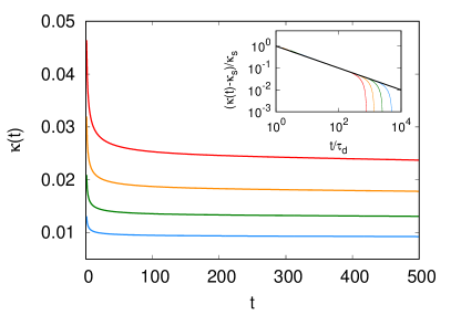
Figure 1: (Color online) Time evolution of the uptake rate $\kappa(t)$ for different values of $\beta$, from top to bottom: $2$ (red), $2\times 10^{-1}$ (orange), $5\times 10^{-2}$ (green) and $2\times 10^{-2}$ (cyan). Inset: $(\kappa(t)-\kappa_{s})/\kappa_{s}$ versus $\tau=t/\tau_{D}$ ($\tau_{D}=R^{2}/(\pi D)$ with $R$ obtained from the fit based on eq. (6)). For short times all the curves collapse on the line $1/\sqrt{\tau}$ (black line) as predicted by (6). Simulations have been performed with resolution $M=64$.

Figure 1 shows the evolution of the uptake rate $\kappa(t)$, computed from (4), as a function of time for different values of $\beta$. Two regimes are observed: at the beginning the diffusive regime described by (6) is well evident (see inset), while for longer times a slower decay due to the boundedness of the domain sets in. By fitting $\kappa(t)$ with the expression (6) in the first regime, one obtains two independent estimated of $R$ (from the constant term and from the time dependent term). For all values of $\beta$ the two measures give the same value of $R$ within $2\%$ of error.

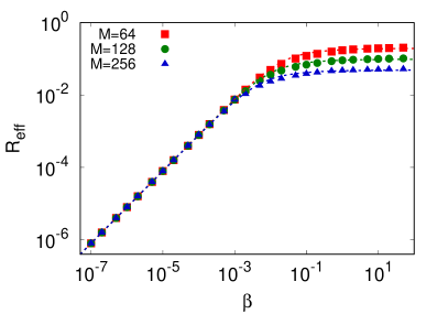
Figure 2: (Color online) Effective radius $R$ obtained from $\kappa(t)$ fitted with (6) versus $\beta$ for different resolutions as labelled. The dashed curves display Eq. (7) with $a=(n/2)\delta x$.

The result of the calibration for the effective radius $R$ is shown in Fig. 2 for different resolutions $M$. For small $\beta$, the effective radius $R$ is proportional to the absorption rate. For large $\beta$, $R$ saturates to $a=(n/2)\delta x$ that depends on the resolution as $n$ is fixed and the mesh size changes as $\delta x=L/M$.
To rationalize this behavior and eventually find an analytical fitting expression for $R$, we resorted to a crude approximation for the regularized delta function assuming a spherical sink function of radius $a$, in polar coordinates $f(r)=\Theta(a-r)/V_{a}$, where $\Theta$ is the Heaviside step function, $r$ the distance from the sphere center and $V_{a}=4\pi a^{3}/3$ the sphere volume. With this form for $f(r)$ the stationary solution of (1) in the infinite space is easily solved (see Appendix B). The analytic expression of the uptake rate (see Eq. (30)), when compared with the Smoluchowski rate, yields

$$R=a-\sqrt{\dfrac{DV_{a}}{\beta}}\tanh\left(a\sqrt{\dfrac{\beta}{DV_{a}}}\right)\,,$$ (7)

which shows a remarkable (within $5\%$) agreement with the effective radius obtained with the fitting procedure (see Fig. 2). Thus Eq. (7) can be used as the calibrating function. Notice that for small $\beta$ Eq. (7) yields $R=\beta/(4\pi D)$, which is the result one would obtain by replacing $f$ with a true $\delta$-function in (4), while $R\to a$ for large $\beta$. Typically, in our simulations we fixed $\beta=D=0.01$ which leads to an effective radius $R\lesssim a$.
It is worth remarking that, as in the case of the Force Coupling Method for fluid-particle interaction Maxey et al. (1997); Lomholt and Maxey (2003), the diffusive boundary layer is not well resolved at the scale of the regularization. This is apparent in Fig. 3, which displays the profile of the scalar field as a function of the distance from the particle. The analytical expression obtained from Eq. (24) agrees well with the numerical result only for $r>2a$, which depends on the resolution, even if $R\ll a$. This, as we will see in the next section, has some repercussions on the ability of the method to resolve the diffusive interactions of close particles.

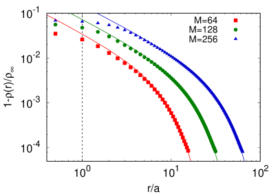
Figure 3: (Color online) Radial profile of the concentration field $\rho(\bm{x},t)$ obtained from simulations at time $t=5\times 10^{4}\tau_{D}$ at varying the resolution as in legend and compared with the theoretical prediction (24) (solid lines). Parameters: $D=10^{-2}$, $\beta=10^{-3}$.

Finally, in Figure 4, we assess possible systematic errors coming from varying the position of the particle in the grid, i.e. errors due to the use of the regularized $\delta$ function (2). We measured the relative error on the uptake rate varying the position of the particle along the side $\delta x$ of a lattice unit, along the face diagonal and along the cube diagonal (see inset). The largest variation observed was less than $1\%$ for a regularization on $n^{3}=64$ grid points.

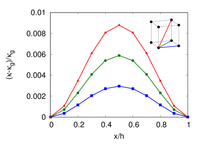
Figure 4: (Color online) Relative error on the uptake rates depending on the position of the particle within the lattice unit. We vary the distance $x$ from a chosen grid point, along three different paths (shown in the inset) of size $h$, from bottom to top: side of the grid unit (blue, $h=\delta x$), face diagonal (green, $h=\sqrt{2}\delta x$) and cube diagonal (red, $h=\sqrt{3}\delta x$). On the $y$-axis we show the discrepancy between the off-grid uptake rate $\kappa$ and the one measured on a grid point $\kappa_{g}$. Along each path, the discrepancy is maximal at the farthest position from the grid. Simulations refer to resolution $M=64$.

III Configurations with multiple absorbers

In this Section we consider $N$ static absorbing particles, arranged in configurations of increasing complexity from regular to random, with the aim of testing the reliability and precision of our method. For the sake of simplicity, we discuss only cases in which all particles have the same radius , i.e. $\beta_{i}=\beta$ in Eq. (1). All simulations are initialized with a uniform scalar field, $\rho(\bm{x},0)=\rho_{0}=1$. The asymptotic uptake rates are evaluated as discussed in Sect. II.1 by fitting $\kappa(t)$ with (6) on each particle. Indeed, it can be shown that the functional form (6) holds also in the case of multiple sinks Traytak (1992, 1995).
We compare the numerically obtained rates with those obtained from a numerical multipole expansion algorithm Galanti et al. (2016). When available, we also compare our results with analytical exact or approximate expressions. The main aim of this study is the validation of our method in resolving the diffusive interaction, quantified by the Sherwood number $Sh$ defined as the total absorption rate normalized with that of $N$ isolated absorbers

$$Sh=\dfrac{\kappa_{tot}}{N\kappa_{s}}\,.$$ (8)

In the last subsection we shall consider the case of a single absorber in the presence of a linear shear flow and study the Sherwood number as a function of the Peclet number, quantifying the ratio between advective over diffusive transport.

III.1 Pairs of absorbers ($N=2$)

The case of two spherical absorbers of radius $R$ separated by a distance $d$ is one of the few examples of diffusive interaction problem that can be solved exactly. After choosing bi-spherical coordinates, the Laplace equation becomes separable Morse and Feshbach (1946) and the total absorption rate depends on the relative distance $x=d/2R$ as Samson and Deutch (1999); Piazza et al. (2005)

$$Sh=\sqrt{x^{2}-1}\sum_{n=0}^{\infty}\frac{2}{1+(x+\sqrt{x^{2}-1})^{2n+1}}\,.$$ (9)

In the limit of well-separated absorbers, $x\to\infty$, Eq. (9) yields the non-interacting result $Sh=1$ (i.e. both spheres absorb the nutrient at the Smoluchovski rate as if they were isolated). Notice that, already for $x\gtrsim 2$ the first correction given by the monopole contribution,

$$Sh=\dfrac{2x}{2x+1}=\dfrac{d}{d+R}\,,$$ (10)

is a very good approximation of (9). In the limit of two spheres in contact, $x=1$, Eq. (9) gives the maximum interference, with $Sh=\ln(2)$.

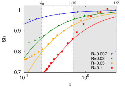
Figure 5: (Color online) $Sh$ as a function of the distance $d$ between two spherical absorbers of radius $R$, varied as in legend. Solid curves represent the exact result (9). The grey shaded regions highlight the range of distances where the numerically obtained $Sh$ becomes sensibly different from the exact value, see text for discussion. The simulations have been performed with $M^{3}=64^{3}$ grid points.

In Fig. 5 we show the numerically computed Sherwood number as a function of the pair distance $d$ for different choices of the particle effective radius $R$ at fixed resolution. The numerical results are directly compared with the exact value obtained from (9). A very good agreement between numerical and theoretical values is observed for distances larger than $d_{m}\approx a=(n/2)\delta x$, and smaller than, about $1/10\div 1/8$ of the domain size $L=2\pi$.
The discrepancies at small distances are due to the fact that the method does not resolve the particle surface: the numerical radius, $a$, imposed by the regularized delta function turns out to be the limiting distance for resolving the pair diffusive interactions (see also Fig. 3 and related discussion), regardless of the effective radius of the particles. To reduce $d_{m}$ the only possibility is thus to increase the resolution.
The large-distance discrepancies are due to the periodicity of the simulation domain. Since the diffusive interactions are long-ranged (they decay with the inverse of the distance from the absorbers, see Eq. (24)), when $d$ increases the particles start to interact not only with each other but also with their periodic images, leading to an increase of the total uptake rate (i.e. $Sh$ becomes larger than predicted for a pair of absorbers at the same distance in the infinite space). This effect tends to increase with the effective radius $R$ of the particle as the diffusive interaction increases with $R$ (see Eq. (24)). We emphasize that this effect cannot be modified by changing the resolution but requires working with different boundary conditions.
Summarizing, the above results show that provided the particles are at distances $(n/2)\delta x=d_{m}<d<d_{M}\approx L/10-L/8$ the numerical method works quite well. Figure 6 shows $Sh$ as function of the rescaled distance $x=d/2R$ together with the exact result and the monopole approximation. As it is clear from the inset, in the whole range of $x$ the numerical values are within $2\%$ from the exact result with larger deviations, $\sim 4\%$, when $x\to 1$ corresponding to distances $d\approx d_{m}$. In the following we shall exploit these results when studying more complex arrangements of absorbing particles, making sure that the particles stay at distances within the range of scales for which the method works well.

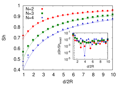
Figure 6: (Color online) $Sh$ for configurations of $N$ equidistant absorbers as a function of the dimensionless distance $x=d/2R$ for $N=2,3,4$ as in legend. Filled symbols are the results from the numerical simulations, open symbols exact results obtained with the method of Ref. Galanti et al. (2016). Lines represent the monopole approximation eq. (12). The inset shows the relative error with respect to the exact solutions. The vertical dashed line is positioned at $x_{m}=d_{m}/2R$, marking the condition for well-resolved simulations. On the left of the threshold line, the error rises to $4-8\%$ while for the other distances it is always close to $1\%$. The resolution used is $M=128$.

III.2 Regular triangles ($N=3$) and tetrads ($N=4$)

We now consider regular arrangements of $N=3$ and $4$ particles at varying distances. From the theoretical side, the monopole expression (10) can be easily extended to the case of $N>2$ absorbers. Within the monopole approximation, one can write the set of linear equations for the uptake rate $\kappa_{i}$ of the $i$-th absorber Traytak (1992, 1995)

$$\kappa_{i}=\kappa^{i}_{s}-\displaystyle\sum_{j\neq i}^{N}\epsilon_{ij}\kappa_{j},\qquad i=1,...,N,$$ (11)

where $\epsilon_{ij}=R_{i}/d_{ij}$, $R_{i}$ is the radius of the $i^{th}$ sphere, $d_{ij}$ the distance between the $i$-th and $j$-th sink and $\kappa^{i}_{s}=4\pi DR_{i}\rho_{\infty}$. The case considered here is $R_{i}=R$ and $d_{ij}=d$, for $N=3,4$. In this limit, the total Sherwood number, in the monopole approximation, is given by ($x=d/2R$):

$$Sh=\dfrac{2x}{2x+(N-1)}\,.$$ (12)

The numerical results are shown in Figure 6, together with the monopole expression (12) and the exact results computed by using the approach described in Ref. Galanti et al. (2016). The limit $x=1$ corresponds to the minimal distance at which the spheres are at contact and therefore to the maximum diffusive interaction. From a numerical standpoint, with our choice of $\beta$, this limit corresponds to $d\approx d_{m}$. The discrepancy between the numerical simulations and the exact results is here maximal, between $4\%$ and $8\%$ (see inset) increasing with $N$ as intuitively expected. At larger distances the exact values are recovered within $\lesssim 2\%$. It is remarkable that the interaction is still observed for $x\simeq 10$, as a consequence of the long-range nature of the diffusive interactions. Notice that, to reach $x=10$ without violating the constraint imposed by the periodic boundary conditions (cfr. Fig. 5), we have varied $x$ also changing the effective radius. We finally remark that as soon as $x>2$ the monopole approximation practically coincides with the exact result.

III.3 Deformed Triangles $N=3$

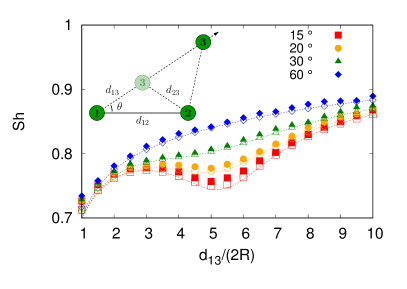
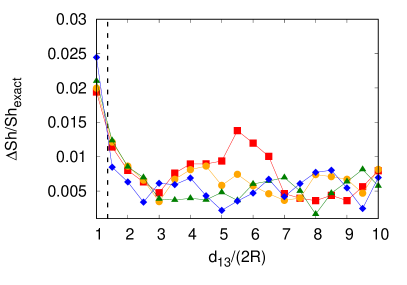
Figure 7: (Color online) Top Panel: $Sh$ for different configurations of deformed triangles with $\theta=15^{\circ},20^{\circ},30^{\circ},60^{\circ}$ as a function of the distance $d_{13}$ normalized by the sphere diameter $2R$. The minimum of $Sh$ corresponds to the configuration of minimal distance $d_{23}$ (filled symbols from the numerical simulations, open symbols obtained with the method of Ref. Galanti et al. (2016)). Inset: Sketch of the deformed triangles. Bottom Panel: relative error of the simulations with respect to the exact results obtained with the method of Ref. Galanti et al. (2016). The dashed line represents the critical distance $x_{m}=d_{m}/(2R)$ below which the numerical accuracy is decreased as discussed in Sect. III.1.

We considered also the case of three spheres of radius $R$ at the vertices of irregular triangles as sketched in the inset of the top panel in Fig. 7. A practical way to construct the triangle is the following: We fix the distance between particle 1 and 2 to be $d_{12}=Xd_{m}$ with $X>1$. Let us denote with $\theta$ the angle between the segments $12$ and $13$. We keep this angle fixed and vary the distance $d_{13}=d$, requiring $d_{ij}\geq d_{m}$ for $i\neq j=1,2,3$, which implies a minimal angle $\theta_{c}=\arcsin(1/X)$. Here we fix $X=5.5$ so that $\theta_{c}\sim 14.35$. In the simulations we used $\theta=15^{\circ},20^{\circ},30^{\circ},60^{\circ}$ and varied $d$ in the range $\in[2R,20R]$. As for the parameters of the simulation we fix $D=\beta=0.01$ in such a way that the radius of the spheres $R=0.036$.
The solution of such configurations in the monopole approximation using Eq. (11) is given by

$$Sh=\dfrac{1}{3}+\dfrac{2}{3}\dfrac{(A-1)(B-1)(C-1)}{A^{2}+B^{2}+C^{2}-2ABC-1},$$ (13)

where $A=R/d_{12}$ with $d_{12}$ fixed, $B=R/d_{13}$ and $C=R/d_{23}$ with $d_{23}=\sqrt{d_{12}^{2}+d_{13}^{2}-2d_{12}d_{23}\cos\theta}$.
In Fig. 7 we plot the total Sherwood number of the triadic system as a function of the distance $d_{13}$ normalized by the diameter of the absorber $2R$. Our simulations, are compared with the exact results obtained following the method of Ref. Galanti et al. (2016). We also compare the results with the monopole approximation (13). The minimal uptake is obtained in the configuration with minimum distance $d_{23}$, which maximizes the diffusive interactions. As shown in bottom panel the error is within $2\%$, but for configurations with $d_{13}\approx d_{m}$, as expected from previous discussions. We conclude by noticing that when particle 3 is moved far away from the pair, we recover the asymptote (not shown) given by the uptake of a single sphere and the contribution of the pair alone, which with our choice is $Sh\simeq 0.94$.

III.4 Random Spherical Cluster

In this Section we consider the case of a cluster of absorbers. One important motivation comes from biology in the case of colonies of microorganisms. In this case one is interested in understanding how diffusive interactions, which cause nutrient shielding for cells in the cluster interior, deplete the growth of the colony Lavrentovich et al. (2013).

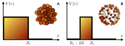
Figure 8: Sketch of the cluster configurations: (A) spherical cluster; (B) sherical shell cluster. The graphs also show the potential used to develop the effective medium approximation.

Specifically, we consider a spherical cluster of absorbers, i.e. a sphere of radius $R_{s}$, centered at the origin, comprising $N$ spherical absorbers, with the same radius $R$, randomly arranged in its interior avoiding geometrical overlaps (see Fig. 8A). In this case it is possible to have an analytical estimation of the nutrient uptake by introducing an effective-medium approximation Lavrentovich et al. (2013).
The basic idea of the method is to introduce an effective concentration field $\psi(\bm{x},t)=\langle\rho(\bm{x},t)\rangle$ where the the brackets denote an ensemble average over the possible random position of the absorbing particles. By averaging both sides Eq. (1) and assuming stationarity, one has

$$D\nabla^{2}\psi=\left\langle\sum_{i=1}^{N}\beta_{i}\rho(\bm{x})\delta(\bm{x}-\bm{X}_{i})\!\!\right\rangle$$ (14)

$$\simeq\int\chi(\bm{x}-\bm{x}^{\prime})\psi(\bm{x}^{\prime})d\bm{x}^{\prime},$$

where $\chi(\bm{x})$ is a linear-response function describing the deformation of the concentration field induced by the absorption Lavrentovich et al. (2013). The linear-response approximation is only valid for sufficiently small concentration field deformations (dilute clusters) and away from the cluster edges. Fourier transforming equation (14), one obtains the equation $-Dq^{2}\hat{\psi}(\bm{q})=\hat{\chi}(\bm{q})\hat{\psi}(\bm{q})$. Since, on average, the cells are isotropically distribuited, $\chi(\bm{q})$ can only depend on $q=|\bm{q}|$. Expanding $\hat{\chi}$ around $q=0$ and truncating at the zeroth order, i.e. $\hat{\chi}(0)=k$, provides the desired mean-field approximation. Hence the configurationally averaged nutrient concentration obeys the equation $D\nabla^{2}\psi-k\psi=0$ valid within the sphere of radius $R_{s}$ delimiting the cluster, outside $D\nabla^{2}\psi=0$, this is nothing but the equation we already solved to determine the calibrating function (7) (see Appendix B). In the above expression $k$ represents an effective absorption rate within the sphere in the macroscopic description. The truncation at zeroth order works reasonably well for dilute clusters, and in this limit $k=4\pi DRN/V_{s}=3D\phi/R^{2}$ where $\phi=NR^{3}/R_{s}^{3}=N/\alpha^{3}$ is the volume fraction (with $\alpha=R_{s}/R$). The cluster is thus approximated as a unique sink with penetrable walls. We can directly use Eq. (30) to express the total uptake rate

$$\kappa_{tot}=4\pi D\psi_{\infty}\left[R_{s}-\xi\tanh\left(\dfrac{R_{s}}{\xi}\right)\right],$$ (15)

$\xi=\sqrt{D/k}=R/\sqrt{3\phi}$ being the penetration length.
The Sherwood number is defined as $Sh=\kappa_{tot}/N\kappa_{s}$, so using $\kappa_{s}=4\pi DR\psi_{\infty}$ and replacing $N=\alpha^{3}\phi$, from (15) we obtain

$$Sh(\phi)=\dfrac{1}{\alpha^{2}\phi}\left[1-\dfrac{1}{\alpha\sqrt{3\phi}}\tanh\left(\alpha\sqrt{3\phi}\right)\right].$$ (16)

Let us now consider the local uptake rate of a cell within the cluster. We denote with $\kappa_{i}$ the uptake rate of the $i$-th particle and we identify its position in the cluster by its distance $r_{i}$ form the center. We can then introduce the average uptake rate $\kappa(r)=\langle\kappa_{i}\big{|}r_{i}=r\rangle$, where the brackets indicate the ensemble average over different configurations. The Sherwood number of a cell at a distance $r$ from the center of the cluster will then be $Sh(r)=\kappa(r)/\kappa_{s}$. By definition, the total uptake rate of the cluster is given by $\kappa_{tot}=\langle\sum_{i}^{N}\kappa_{i}\rangle$, while the total flux absorbed by the particles contained in a smaller sphere of radius $r$ is given by

$$4\pi Dr^{2}\dfrac{d\psi}{dr}=N\int_{0}^{r}\kappa(r^{\prime})p(r^{\prime})dr^{\prime},$$ (17)

where $p(r)dr=V_{s}^{-1}4\pi r^{2}\theta(R_{s}-r)dr$ is the probability to find a particle at a certain radial position. By taking the derivative of expression (17), one gets

$$Sh(r)=\dfrac{\xi^{2}}{\psi_{\infty}r^{2}}\dfrac{d}{dr}\left(r^{2}\dfrac{d}{dr}\psi\right).$$ (18)

By noting that $\xi^{2}\nabla^{2}\psi=\psi$, it’s easy to see that $Sh(r)=\psi(r)/\psi_{\infty}$, i.e. the local uptake rate $\kappa(r)$ is proportional to the averaged concentration profile $\psi(r)$.
We turn now to the numerical results. We considered random distribution of particles in a spherical cluster of radius $R_{s}=L/8=\pi/4$ so to minimize effects due to the periodic boundary conditions (cfr. Fig. 5). As for the absorbers, we considered $N=20,50,100,150$ spheres with effective radius $R\sim 0.036$ so that the (nominal) volume fraction ranges in $\phi=2\cdot 10^{-3}-10^{-2}$, that is, small enough for the effective medium approximation to be accurate. Particles are placed uniformly within the sphere volume, ensuring that they stay at distances larger than $d_{m}\approx(n/2)\delta{x}=(n/M)\pi$ to reduce the errors due to poor resolution of the diffusive interaction at short distances (Cfr. Fig. 5). For each $N$ we considered from $5$ to $10$ different configurations to perform ensemble averages and thus to compare with the effective field approximation. The same configurations have been used to compute the exact solution with the method of Ref. Galanti et al. (2016).

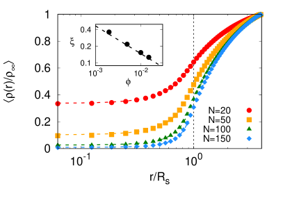
Figure 9: (Color online) Average radial concentration profile $\langle\rho(r)\rangle$ vs $r/R_{s}$, for clusters with $N=20,50,100,150$ particles as labeled. Numerical data (symbols) are compared with the effective medium solution given by eq. (29) (dashed curves). Inset: Penetration length $\xi$ obtained from the fit of the radial profile (filled circles) and theoretical prediction given by $\xi=R/\sqrt{3\phi}$ Traytak (2013) (dashed line). The average is performed over $5-20$ independent realizations. The numerical resolution is $M=128$.

Figure 9 shows the average density profile $\psi(r)=\langle\rho(r)\rangle$ compared with the theoretical prediction given by the effective medium approximation (29). The agreement is remarkably good.
From the simulations, we can extract the uptake rate of each particle using the standard fitting procedure, which involves the temporal evolution of uptake rate at intermediate times (see Sect. II.1). By averaging over particles and different configurations, one obtains a measure of the total uptake rate of the cluster. Alternatively, one can extract the uptake rate of the cluster directly from the concentration field $\rho$. The radial profile can be compared with the theoretical prediction (29) to extract the parameters of interest. From the inner solution it is possible to extrapolate the penetration length $\xi$ shown in the inset of Fig. 9 with the scaling $R/\sqrt{3\phi}$. By fitting the behavior in the outer region, we have an alternative estimate of the total Sherwood number.
In Figure 10 we plot the individual Sherwood number $Sh_{i}=\kappa_{i}/\kappa_{s}$ as a function of the radial distance of particles in the cluster, compared with the values obtained from the exact numerical solution. The relative difference is below $8\%$, as shown in the inset, and is larger in the interior of the cluster, due to the accumulation of errors on the concentration density due to the outer absorbers. In Fig.10 we also plot the theoretical prediction (18).
Finally, in Fig. 11 we show that also the total Sherwood number compare very well with the theoretical prediction (16) and the exact computation (with error within $10\%$).

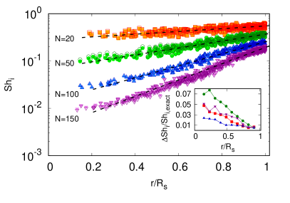
Figure 10: (Color online) Individual Sherwood number $Sh_{i}=\kappa_{i}/\kappa_{s}$ for absorbers in a spherical cluster with $N$ particles as labeled. Filled symbols denote the numerical results obtained by our numerical method, empty symbols those obtained with the exact numerical computation described in Ref. Galanti et al. (2016). Dashed lines represents the prediction (18). Inset: relative errors of the uptake computed as the average absolute distance of the two numerical methods, plotted as a function of the radial coordinate.

III.5 Spherical Shell Cluster

In this section we study a generalization of the spherical cluster, considering absorbers with their centers at a fixed distance from the origin of the sphere of radius $R_{s}$ (see Fig. 8b). This kind of configuration is encountered in nature. For example, Volvox is a colonial alga forming spherical colonies with a $1$-mm diameter, is usually $100$ times larger than the single cell forming it and contains up to $5\,10^{4}$ cells organized as a monolayer of flagellated cells on the sphere surface Miller (2010).
Following the same idea used for developing the effective medium approximation of spherical cluster, one can develop an analytical description for spherical shell clusters. In particular, after averaging over the absorbers configurations and performing the expansion of the response function we end up with the equation:

$$D\nabla^{2}{\psi}=k[\Theta(R_{s}-|\bm{r}|)+\Theta(|\bm{r}|-(R_{s}-2R))]\psi,$$ (19)

$\Theta$ being the Heavyside step function. The above equation must be solved with the boundary condition $\psi(r\to\infty)=\psi_{\infty}$ and where again $k=3D\phi/R^{2}$ in the dilute limit. Now the volume fraction is given by $\phi=NV_{p}/V_{s}$ with $V_{p}=4\pi R^{3}/3$ the volume of the single absorber and $V_{s}$ the volume of the shell between $R_{s}-2R$ and $R_{s}$. The solution of Eq. (19) is detailed in Appendix C.
Similarly to the previous section, introducing $\alpha=R_{s}/R$ and $N=\phi V_{s}/V_{p}=2\phi(3\alpha^{2}-6\alpha+4)$, and using the expression for the total uptake rate Eq. (32), after some algebra, the total Sherwood number can be expressed as

$$Sh(\phi)=\dfrac{\frac{1}{2}[\alpha(\alpha-2)\sqrt{3\phi}-1/\sqrt{3\phi}]\tanh(2\sqrt{3\phi})\!+\!1}{\phi(3\alpha^{2}-6\alpha\!+\!4)[(\alpha-2)\sqrt{3\phi}\tanh(2\sqrt{3\phi})\!+\!1]}.$$ (20)

In Fig. 11 the total Sherwood number is compared with the theoretical prediction (20), the agreement is good within $10\%$. It is also interesting to note that the present configuration in spherical shell-like geometry enhances the uptake rates per cell and the total uptake rates of the cluster with respect to the configurations of bulk spherical clusters. Therefore, it can represent an efficient strategy to maximize the uptake rate.

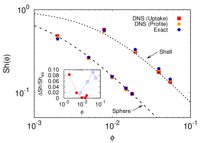
Figure 11: Total normalized Sherwood number $Sh=\kappa/N\kappa_{s}$ for the spherical cluster and spherical shell as a function of the volume fraction $\phi$, averaged over 5 to 10 configurations and obtained by fitting the instantaneous uptake (red squares) or fitting the outer solution of the radial concentration profile (orange circles). Simulations are compared with exact results calculated using the method described in Ref. Galanti et al. (2016) (blue pentagons). Inset: Relative error between simulations and exact results for the spherical cluster (filled circles) and for the spherical shell (empty circles).

IV Spherical absorber in a linear shear flow

We end testing the method in the presence of a flow, we consider a single (non-rotating) absorber of radius $R$ placed in the position of zero velocity (so that it does not move) of a linear shear, ${\bm{u}}=\gamma(y,0,0)$, for which analytical results are available Leal (2007); Karp-Boss et al. (1996). Nutrient evolves according to Eq. (1) with the addition of the advection term:

$$\partial_{t}\rho+\bm{u}\cdot\bm{\nabla}\rho=D\nabla^{2}\rho-\rho\sum_{i}^{N}\beta_{i}\,f(\bm{x}-\bm{X}_{i})\,.$$ (21)

Analytical results predicts that for small Peclet numbers , $Pe=\gamma R^{2}/D$ , the Sherwood number behaves as Frankel and Acrivos (1968); Karp-Boss et al. (1996)

$$Sh\approx 1+0.26Pe^{1/2}\,.$$ (22)

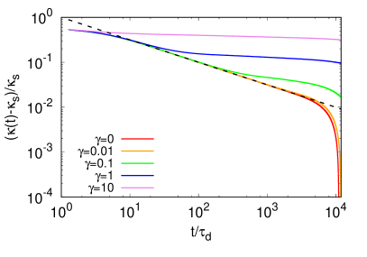
Figure 12: (Color Online) Time evolution of the uptake rate $\kappa(t)$ rescaled by the diffusive uptake rate $\kappa_{s}$ for different values of $\gamma$ (decreasing from top to bottom) at fixed particle radius $R=0.05$ ($\beta=D=0.01$). Resolution $M=64$.

Before presenting the results of simulations of Eq. (21), we discuss the relevant scales for well-resolving the competition between shear and diffusion. Shear and diffusion balance at a scale $\ell_{\gamma}\sim\sqrt{D/\gamma}$, diverging for $\gamma\to 0$. Stationarity (in the infinite volume) is reached when the diffusive front becomes comparable with the scale $\ell_{\gamma}$, i.e. for times $\tau_{\gamma}\sim\ell_{\gamma}^{2}/D=\gamma^{-1}$, also diverging for $\gamma\to 0$. Thus $\ell_{\gamma}$ should be much smaller than the simulation box $L$ otherwise the effect of shear starts to be effective over time scales for which the absorber is also interacting with its periodic images. The requirement $\ell_{\gamma}\ll L$ implies a constraint on the smallest shear rate that can be used, i.e. $\gamma\gg D/L^{2}$. Moreover, since we are interested in testing the prediction (22) for $Pe=\gamma R^{2}/D\ll 1$, we end up with the requirements: $D/L^{2}\ll\gamma\ll D/R^{2}$ that can be re-expressed as $R^{2}/D=\tau_{d}\ll\tau_{\gamma}\ll\tau_{L}=L^{2}/D$ and $R\ll\ell_{\gamma}\ll L$ in the time and scale domain, respectively.

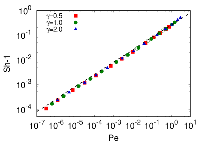
Figure 13: (Color Online) Shear contribution to the Sherwood number $Sh$ as a function of Peclet number $Pe$ for numerical simulations at two different resolutions: M=64 (filled symbols) and M=128 (empty symbols). The line represents the theoretical behavior (22). The Peclet number $Pe$ is changed by fixing the shear rate $\gamma$ and varying the radius $R$.

The limitation on the smallest value of $\gamma$ is well evident from Fig. 12, where we show the time evolution of the uptake rate, $\kappa(t)$, at varying $\gamma$ when $D$ and $R$ are fixed. For time $t\ll\tau_{\gamma}$ $\kappa(t)$ is essentially indistinguishable from that obtained in the diffusive case ($\gamma=0$). For $\gamma\lesssim 0.01$, $\tau_{\gamma}$ is comparable with the time at which the decay induced by the absorber periodic images becomes effective. Figure 12 also show that, due to the shear, the time behavior of the uptake rate is quite different from the Smoluchovsky (diffusive) result, Eq. (6). As a consequence, we cannot exploit (6) to fit the rate, as previously done. Without a theoretical prediction for $\kappa(t)$, we can extract the (infinite volume) uptake rate constant using Eq. (5). Assuming a constant uptake rate $\kappa$, the mean concentration should decay linearly in time as $C(t)=C_{0}-(\kappa/V)t$ with $V=L^{3}=(2\pi)^{3}$. The above functional form should be fitted in the time interval $\tau_{\gamma}<t<\tau_{L}$, when the disturbance induced by the shear is well-developed and (quasi-)stationary. In order to test the prediction (22) we proceed as follows. Given the diffusion coefficient $D$, we fixed the shear rate $\gamma$ at three representative values, such that $\ell_{\gamma}$ is well resolved by the numerical grid and $\ell_{\gamma}\ll L$. Then we explored different values of Peclet number $Pe$ by varying the particle radius $R$ (viz. the absorption rate $\beta$), but enforcing the constraint $\ell_{\gamma}\gg R$ to have a small $Pe$. We performed two series of simulations using grid resolution $M=64,128$. For each series of simulations we explore a sufficiently wide range of values of Peclet number, fitting the uptake rate constant as described above. As shown in Figure 13, the excess Sherwood number, $Sh-1$, as a function of $Pe$ compares very well with (22).

V Conclusions

We presented a novel numerical method for computing the nutrient uptake rate by small spherical particles immersed in a concentration field, in the diffusion-limited regime. The method, inspired by the Force Coupling Method, represents each particle as an effective sink of concentration and can in principle be used in presence of a generic underlying flow, motile particles, and source terms for the concentration field. Moreover, more complex reaction scheme can be easily implemented to mimic partial or saturable absorption.
By comparing the numerical results with exact results obtained from a multipole expansion method based on re-expansion formulae for solid harmonics, we have shown that the method, here implemented on a pseudo-spectral solver, is able to correctly reproduce the diffusive interactions among competing absorbers arranged in geometrical configurations of increasing complexity. As discussed the main limitation of the method resides on the possibility to resolve diffusive interactions at small distances, but this can be cured increasing the resolution. Another limitation pertain to the large distances, but this is only due to the periodicity of the simulation domain and thus it does not concern the method itself.
The main advantages of the method are the scalability with the number of absorbers and the possibility to include the presence of an arbitrary flow, for which we show a benchmark in the case of a linear shear. These properties make our numerical method ideal for the study of problems possibly involving complex, turbulent flows, such as the efficiency of nutrient uptake by microorganisms in the ocean. In future investigations we plan to implement the presented method to particles transported by turbulent flows, back-reacting on it and possibly equipped with self-propulsion.

Appendix A Smoluchowski Formula

The problem of diffusion-limited reaction was first studied by Smoluchowski Smoluchowski (1917) and then applied to the heat flow into a sphere with a constant temperature Carslaw and Jaeger (1959). In the ecology of phytoplankton the model was first introduced by Osborn Osborn (1996). In the absence of a flow, the uptake by a single spherical cell is controlled by the diffusion equation

$$\partial_{t}\rho=D\nabla^{2}\rho$$ (23)

where D is the diffusivity and boundary conditions (for a perfect absorber) are $\rho=0$ at $r=R$ and $\rho=\rho_{\infty}$ as $r\rightarrow\infty$.
Using the Laplace transform, equation (23) gives the solution

$$\rho(r,t)=\rho_{\infty}\left[1-\frac{R}{r}\operatorname{Erfc}\left(\frac{r-R}{2\sqrt{Dt}}\right)\right]$$ (24)

The flux per unit area is $J(r,t)=-D\partial_{r}\rho$. Integrated over the solid angle at $r=R$, this gives the rate of nutrient flux entering into the cell surface, i.e. $\kappa(t)=J(R,t)\,4\pi R^{2}$. Therefore, from (24), the uptake rate at the sphere is

$$\kappa(t)=4\pi DR\rho_{\infty}\left(1+\frac{R}{\sqrt{\pi Dt}}\right)$$ (25)

In the limit of long times $t\rightarrow\infty$, $\kappa(t)$ reduces to the Smoluchowski constant rate $\kappa_{s}$.

Appendix B The mean-field theory of absorption by a spherical potential

Here we aim at solving the following equation:

$$\nabla^{2}\varphi-k\Theta(b-|\bm{r}|)\varphi=0\,,$$ (26)

with the boundary condition $\varphi(|\bm{r}|\to\infty)=\varphi_{\infty}$, and where $\Theta$ is the Heaviside function. The solution we are interested in is spherically symmetric so, denoting $r=|\bm{r}|$, the equation we actually need to solve is:

$$\varphi^{\prime\prime}+2\varphi^{\prime}/r-\varphi/\xi^{2}=0\,,$$ (27)

where $\xi=\sqrt{D/k}$ has dimensions of a length, and the prime denotes the derivative with respect to $r$. The general solution is Polyanin and Zaitsev (1995)

$$\varphi=\left\{\begin{array}[]{ll}\frac{C_{1}\xi\sinh(r/\xi)+C_{2}\xi\cosh(r/\xi)}{r}&r\leq b\\ \frac{C_{3}}{r}+\varphi_{\infty}&r\geq b\,.\end{array}\right.$$ (28)

To avoid a singular solution in $r=0$ we impose $C_{2}=0$, while $C_{1}$ and $C_{3}$ can be fixed imposing continuity of $\varphi$ and its derivative in $r=b$. The final result is:

$$\varphi(r)=\left\{\begin{array}[]{ll}\frac{\varphi_{\infty}\xi}{\cosh(b/\xi)}\frac{\sinh(r/\xi)}{r}&r\leq b\\ \varphi_{\infty}\left(1-\frac{b-\xi\tanh(b/\xi)}{r}\right)&r\geq b\,.\end{array}\right.$$ (29)

For the results presented in the main text we need to compute the flux on the surface of the sphere of radius $b$, which is simply obtained as:

$$\kappa=4\pi Dr^{2}\left.\frac{\partial\varphi}{\partial r}\right|_{r=b}=4\pi D\varphi_{\infty}\left[b-\xi\tanh(b/\xi)\right]$$ (30)

Appendix C The absorption by a spherical shell potential

Here we aim at solving equation (19). Similarly to the case discussed in Appendix B (see Eq. (28), we have three regions with different solutions. In the interior of the shell, for $r<R_{s}-2R$, we have the solution $\psi_{I}=a_{1}+b_{1}\xi/r$, clearly $b_{1}=0$ due to the divergence at $r=0$. In the region $R_{s}-2R<r<R_{s}$ the solution is $\psi_{II}=(\xi/r)(a_{2}e^{r/\xi}+b_{2}e^{-r/\xi})$. In the outer region, $r>R_{s}$, the solution is $\psi_{III}=a_{3}+b_{3}\xi/r$.
The boundary condition at infinity implies that $a_{3}=\psi_{\infty}$. Imposing the continuity of the solution and its derivative at $r=R_{s}-2R$ and $r=R_{s}$ we obtain the remaining unknown constants. The final solution is

$$\dfrac{\psi(x)}{\psi_{\infty}}=\left\{\begin{array}[]{ll}\dfrac{1}{X_{1}\sinh\left(X\right)\!+\!\cosh\left(X\right)}&(I)\\[14.22636pt] \dfrac{1}{x}\dfrac{X_{1}\cosh\left(x\!-\!X_{1}\right)+\sinh\left(x\!-\!X_{1}\right)}{X_{1}\sinh\left(X\right)\!+\!\cosh\left(X\right)}&(II)\\[14.22636pt] 1\!-\!\dfrac{1}{x}\dfrac{\left(X_{1}X_{2}\!-\!1\right)\tanh\left(X\right)\!+\!X}{X_{1}\tanh\left(X\right)\!+\!1}&(III)\end{array}\right.$$ (31)

where $x=r/\xi$, $X=2R/\xi$,a $X_{1}=(R_{s}-2R)/\xi$, $X_{2}=R_{s}/\xi$ and the three regions correspond to: $I=[0,X_{1}]$, $II=[X_{1},X_{2}]$ and $III=[X_{2},\infty)$.
As before, the total uptake rate at $r=R_{s}$ is given by

$$\kappa_{tot}=4\pi Dr^{2}\left.\frac{\partial\psi}{\partial r}\right|_{r=R_{s}}=4\pi Db_{3}\xi\,,$$ (32)

where $b_{3}$ can be read from the term proportional to $1/x$ in (31).III.

References

- Rice (1985) S. A. Rice, Diffusion-limited reactions, Vol. 25 (Elsevier, 1985).
- Berg (1993) H. C. Berg, Random walks in biology (Princeton University Press, 1993).
- Karp-Boss et al. (1996) L. Karp-Boss, E. Boss, P. Jumars, et al., Oceanogr. Mar. Biol. 34, 71 (1996).
- Kiørboe (2008) T. Kiørboe, A mechanistic approach to plankton ecology (Princeton University Press, 2008).
- Leal (2007) L. G. Leal, Advanced transport phenomena: fluid mechanics and convective transport processes (Cambridge University Press, 2007).
- Neufeld and Hernández-García (2009) Z. Neufeld and E. Hernández-García, Chemical and Biological Processes in Fluid Flows: A Dynamical Systems Approach (World Scientific, 2009).
- Fournier-Bidoz et al. (2005) S. Fournier-Bidoz, A. C. Arsenault, I. Manners, and G. A. Ozin, Chem. Commun. 4, 441 (2005).
- Ozin et al. (2005) G. A. Ozin, I. Manners, S. Fournier-Bidoz, and A. Arsenault, Adv. Mater. 17, 3011 (2005).
- Golestanian et al. (2007) R. Golestanian, T. Liverpool, and A. Ajdari, New J. Phys. 9, 126 (2007).
- Smoluchowski (1917) M. V. Smoluchowski, Colloid Polym. Sci. 21, 98 (1917).
- Traytak (1992) S. Traytak, Chem. Phys. Lett. 197, 247 (1992).
- Traytak (1995) S. Traytak, Chem. Phys. 193, 351 (1995).
- Dorsaz et al. (2010) N. Dorsaz, C. De Michele, F. Piazza, P. De Los Rios, and G. Foffi, Phys. Rev. Lett. 105, 120601 (2010).
- Lavrentovich et al. (2013) M. O. Lavrentovich, J. H. Koschwanez, and D. R. Nelson, Phys. Rev. E 87, 062703 (2013).
- Galanti et al. (2016) M. Galanti, D. Fanelli, S. D. Traytak, and F. Piazza, Phys. Chem. Chem. Phys. 18, 15950 (2016).
- Kalay et al. (2012) Z. Kalay, T. K. Fujiwara, and A. Kusumi, PLoS ONE 7 (2012).
- Grima and Schnell (2006) R. Grima and S. Schnell, Biophys. Chem. 124, 1 (2006).
- Kusumi et al. (2012a) A. Kusumi, T. K. Fujiwara, R. Chadda, M. Xie, T. A. Tsunoyama, Z. Kalay, R. S. Kasai, and K. G. N. Suzuki, Annu. Rev. Cell Dev. Biol. 28, 215 (2012a).
- Sourjik (2004) V. Sourjik, Trends Microbiol. 12, 569 (2004).
- O’Connell et al. (2006) K. M. S. O’Connell, A. S. Rolig, J. D. Whitesell, and M. M. Tamkun, J. Neurosci. 26, 9609 (2006).
- Kusumi et al. (2012b) A. Kusumi, T. K. Fujiwara, N. Morone, K. J. Yoshida, R. Chadda, M. Xie, R. S. Kasai, and K. G. N. Suzuki, Semin. Cell Dev. Biol. 23, 126 (2012b).
- Bálint et al. (2017) Š. Bálint, M. L. Dustin, A. Bruckbauer, F. Batista, S. Banjade, J. Okrut, D. King, J. Taunton, M. Rosen, R. Vale, Z. Guo, R. Vishwakarma, M. Rao, S. Mayor, D. Klenerman, A. Aricescu, and S. Davis, eLife 6, 1055 (2017).
- Shukla et al. (2014) A. K. Shukla, G. Singh, and E. Ghosh, Trends Biochem. Sci. 39, 594 (2014).
- Eun et al. (2013) C. Eun, P. M. Kekenes-Huskey, and J. A. McCammon, J. Chem. Phys. 139, 07B623_1 (2013).
- Felderhof et al. (1982) B. Felderhof, J. Deutch, and U. Titulaer, J. Chem. Phys. 76, 4178 (1982).
- Muthukumar (1982) M. Muthukumar, J. Chem. Phys. 76, 2667 (1982).
- Bonnecaze and Brady (1991) R. Bonnecaze and J. F. Brady, J. Chem. Phys. 94, 537 (1991).
- Richards (1987) P. M. Richards, Phys. Rev. B 35, 248 (1987).
- Lee et al. (1989) S. B. Lee, I. C. Kim, C. A. Miller, and S. Torquato, Phys. Rev. B 39, 11833 (1989).
- Tsao et al. (2001) H.-K. Tsao, S.-Y. Lu, and C.-Y. Tseng, TJ. Chem. Phys. 115, 3827 (2001).
- Traytak (2003) S. D. Traytak, J. Comp. Mech. Des. 9, 495 (2003).
- Morse and Feshbach (1946) P. M. Morse and H. Feshbach, Methods of theoretical physics (Technology Press, 1946).
- Gordeliy et al. (2009) E. Gordeliy, S. L. Crouch, and S. G. Mogilevskaya, Int. J. Numer. Methods Eng. 77, 751 (2009).
- Lambert et al. (2013) R. A. Lambert, F. Picano, W.-P. Breugem, and L. Brandt, J. Fluid Mech. 733, 528 (2013).
- Musielak et al. (2009) M. M. Musielak, L. Karp-Boss, P. A. Jumars, and L. J. Fauci, J. Fluid Mech. 638, 401 (2009).
- Peskin (2002) C. S. Peskin, Acta Numerica 11, 479 (2002).
- Maxey et al. (1997) M. Maxey, B. Patel, E. Chang, and L.-P. Wang, Fluid Dyn. Res. 20, 143 (1997).
- Lomholt and Maxey (2003) S. Lomholt and M. R. Maxey, J. Comput. Phys. 184, 381 (2003).
- Lomholt et al. (2002) S. Lomholt, B. Stenum, and M. Maxey, Int. J. Multiphase Flow 28, 225 (2002).
- Pal Singh Bhalla et al. (2013) A. Pal Singh Bhalla, B. E. Griffith, N. A. Patankar, and A. Donev, J. Chem. Phys. 139, 214112 (2013).
- Frankel and Acrivos (1968) N. A. Frankel and A. Acrivos, Phys. Fluids 11, 1913 (1968).
- Samson and Deutch (1999) R. Samson and J. Deutch, J. Chem. Phys. 67, 847 (1999).
- Piazza et al. (2005) F. Piazza, P. De Los Rios, D. Fanelli, L. Bongini, and U. Skoglund, Eur. Biophys. J. 34, 899 (2005).
- Traytak (2013) S. D. Traytak, Phys. Biol. 10, 045009 (2013).
- Miller (2010) S. M. Miller, Nature Edu. 3, 65 (2010).
- Note (1) N.A. Frankel and A. Acrivos (1968) attain the result , by defining (the homolog of for the heat transfer) based on the particle diameter, and with . Transforming in our variables and , we obtain the relation , with .
- Carslaw and Jaeger (1959) H. S. Carslaw and J. C. Jaeger, Oxford: Clarendon Press (1959).
- Osborn (1996) T. Osborn, J. Plankton Res. 18, 185 (1996).
- Polyanin and Zaitsev (1995) A. D. Polyanin and V. F. Zaitsev, Chapman and Hall/CRC 2 (1995).