Moving Horizon Estimation for ARMAX process with t -Distribution Noise

Abstract

In this paper, instead of the usual Gaussian noise assumption, $t$-distribution noise is assumed. A Maximum Likelihood Estimator using the most recent N measurements is proposed for the Auto-Regressive-Moving-Average with eXogenous input (ARMAX) process with this assumption. The proposed estimator is robust to outliers because the ‘thick tail’ of the t-distribution reduces the effect of large errors in the likelihood function. Instead of solving the resulting nonlinear estimator numerically, the Influence Function is used to formulate a computationally efficient recursive solution, which reduces to the traditional Moving Horizon Estimator when the noise is Gaussian.The formula for the variance of the estimate is derived. This formula shows explicitly how the variance of the estimate is affected by the number of measurements and noise variance. The simulation results show that the proposed estimator has smaller variance and is more robust to outliers than the Moving Window Least-Squares Estimator. For the same accuracy, the proposed estimator is an order of magnitude faster than the particle filter.

, , ,

1 Introduction

Gaussian noise is often assumed in state estimation. However, the Gaussian noise assumption is an approximation to reality. The occurrence of outliers, transient data in steady-state measurements, instrument failure, model nonlinearity, etc. can all induce non-Gaussian data [16].

It is well-known that the $\it t$-distribution has the property of ‘ thick tail’  to better model the occurence of outliers [10]. In addition, as a special case, the $\it t$-distribution reduces to the Gaussian distribution when its degree of freedom tends to infinity. Thus the $\it t$-distribution has the flexibility to characterize noise with Gaussian or non-Gaussian statistical properties. In the literature the heavy tail property of the $\it t$-distribution has been used to improve the performance of estimators in [13, 2, 1, 15]. These papers are based on the Bayesian method and the heavy tail property of $t$-distribution was used to reduce the effect of outliers. Our method differs from these estimators in that the probability density function (pdf) of the $\it t$-distribution is used directly in the likelihood function for a Maximum Likelihood Estimator (MLE).

The sensitivity of an estimator when the underlying noise assumption (such as Gaussian noise) is violated has been extensively studied in the robust statistics literature [9, 6, 8, 12]. In particular, Huber [9] studied the effect of outliers by contaminating the underlying noise distribution with data from an arbitrary unknown distribution. Hampel [6] proposed the Influence Function (IF) approach to describe the effect of an infinitesimal contamination of the underlying noise distribution. If the IF of an estimator is bounded and/or decreasing, or increasing slowly for large magnitude of noise, then the estimator is robust to outliers. It can be shown that the IF of the least-squares estimator increases linearly with the magnitude of noise and is unbounded [6]. This confirms the well-known fact that standard least-squares estimation is not robust to outliers. Other approaches for handling non-Gaussian noise include the particle filter [3] which is based on the Monte Carlo method, but at the expense of a heavier computational load.

IF has been mainly used as an analysis tool. The main contribution of this paper, Theorem 6, is to employ the IF for state estimation. We formulate a computationally efficient recursive algorithm that gives an approximate solution to the moving horizon MLE for Auto-Regressive-Moving-Average with eXogenous inputs (ARMAX) process with $t$-distribution noise.

ARMAX processes are popularly used in the statistical analysis of time series [4]. The Kalman filter for an ARMAX process is well-known, see Example 11.6 in [4]. In [7] a MLE of an ARMAX process with generalized $t$-distribution noise was developed. However, in [7] the IF was used to approximate the MLE by using all the measurements. This makes the estimator insensitive to plant parameter changes [11]. In this paper we derive the moving horizon version of the ARMAX filter. We derive a computationally efficient recursive algorithm in Section 3. We also analyze the statistical properties of the proposed estimator in Section 4. More specifically, the formula for the variance of the estimate is derived.

2 Maximum Likelihood Estimation and its approximation for ARMAX process with $t-$distribution noise

Consider the following single-input single-output ARMAX process:

$$A\left(q^{-1}\right)y_{k}=B\left(q^{-1}\right)u_{k}+C\left(q^{-1}\right)e_{k},$$ (1)

where $k$ is the sampling instance, $u_{k}$ and $y_{k}$ are the input and output respectively. The polynomials are assumed to be co-prime and given as

$$A\left(q^{-1}\right) = 1+a_{1}q^{-1}+\cdots+a_{n}q^{-n},$$

$$B\left(q^{-1}\right) = b_{1}q^{-1}+b_{2}q^{-2}+\cdots+b_{n_{B}}q^{-n_{B}},$$

$$C\left(q^{-1}\right) = 1+c_{1}q^{-1}+\cdots+c_{n}q^{-n},$$

where $n_{B}\leqslant n$ and $q^{-1}$ is the backward shift operator, i.e., $q^{-1}y_{k}=y_{k-1}$. The zeros of the polynomials $A(q^{-1})$ and $C(q^{-1})$ are inside the unit disc. $e_{k}$ is an independent and identically distributed random variable associated with the zero mean $t$-distribution pdf [10]

$$f(e_{k})=\frac{{\bf\Gamma}\left(\frac{\nu+1}{2}\right)}{\sqrt{\nu\pi}\sigma{\bf\Gamma}\left(\frac{\nu}{2}\right)}\left(1+\frac{e_{k}^{2}}{\sigma^{2}\nu}\right)^{-\frac{\nu+1}{2}}\triangleq t_{\nu}\left(0,\sigma\right)$$ (2)

The degree of freedom and scale parameters are given by $\nu$ and $\sigma$ respectively, and ${\bf\Gamma}$ is the gamma function.

For convenience, we will derive the estimator in state-space form. The ARMAX process (1) in minimal state-space form is given as [4]

$$x_{k+1} = \Phi_{a}x_{k}+\Gamma u_{k}+\Omega e_{k},$$ (3a)

$$y_{k} = Hx_{k}+e_{k},$$ (3b)

where

$$\Phi_{a} = \left[\begin{matrix}-a_{1}&1&0&0&\cdots&0&0\\ -a_{2}&0&1&0&\cdots&0&0\\ \vdots&\vdots&\vdots&\vdots&\ddots&\vdots&\vdots\\ -a_{n-1}&0&0&0&\cdots&0&1\\ -a_{n}&0&0&0&\cdots&0&0\end{matrix}\right]~{}\Gamma=\left[\begin{matrix}b_{1}\\ b_{2}\\ \vdots\\ b_{n_{B}}\\ 0\end{matrix}\right],$$

$$\Omega = \left[\begin{matrix}c_{1}-a_{1}&c_{2}-a_{2}&\cdots&c_{n}-a_{n}\end{matrix}\right]^{{}^{\prime}},H=\left[\begin{matrix}1&0&\cdots&0\end{matrix}\right].$$

2.1 Maximum Likelihood Estimation

Given measurements $y_{1},~{}y_{2},~{}\cdots,~{}y_{{}_{T}}$, we denote the MLE of $x_{1}$ for the ARMAX process (3) with $t$-distribution noise as

$$\hat{x}_{{}_{\rm MLE}}=\arg~{}\!\min_{\hat{x}_{1}}J,$$ (4)

where

$$J = -\textstyle{\sum_{k=1}^{T}}\ln f(e_{k}),$$ (5a)

$$e_{k} = y_{k}-H\Phi^{k-1}\hat{x}_{1}-Hs_{k},$$ (5b)

$$\Phi = \Phi_{a}-\Omega H,$$ (5c)

$$s_{k} = \begin{cases}{\bf 0}&{\rm if}~{}k=1,\\ \textstyle{\sum_{i=1}^{k-1}}\Phi^{k-i-1}\left(\Gamma u_{i}+\Omega y_{i}\right)&{\rm if}~{}k\geqslant 2.\end{cases}$$ (5d)

Then the solution to (4) can be found by solving the equation

$$\textstyle{\sum_{k=1}^{T}}\psi_{k}(e_{k})=0,$$ (6)

where $\psi_{k}(e_{k})\triangleq\frac{d}{d\hat{x}_{1}}\left(-\ln f\left(e_{k}\right)\right)=-\frac{\left(\nu+1\right)\left(H\Phi^{k-1}\right)^{{}^{\prime}}e_{k}}{\sigma^{2}\nu+(e_{k})^{2}}$.

Definition 1.

Influence Function [6].
The IF of an estimator $G$ at distribution $F$ is

$${\rm IF}\left(y;G,F\right)=\mathop{\lim}_{h\rightarrow 0}\frac{G\left((1-h)F+h\Delta_{y}\right)-G(F)}{h},$$

where $h\in[0,1]$ and $\Delta_{y}$ denotes the probability measure which puts mass 1 at the point $y$.

The IF describes the effect of an infinitesimal contamination at the point $y$ on the estimate, standardized by the mass of the contamination. In this paper the noise is assumed to be $t$ distributed with pdf $f(e_{k})$. Taking the expectation of (6) gives

$$\textstyle{\sum_{k=1}^{T}}\textstyle{\int_{-\infty}^{\infty}}\psi_{k}\left(e_{k}\right)f\left(e_{k}\right)de_{k}=0.$$ (7)

Now we wish to obtain the IF of our estimator. As a first step, we replace $f(e_{k})$ in (7) with $(1-h)f\left(e_{k}\right)+h\Delta_{e_{k}}$

$$\textstyle{\sum_{k=1}^{T}\int_{-\infty}^{\infty}}\psi_{k}\left(e_{k}\right)\left[(1-h)f\left(e_{k}\right)+h\Delta_{e_{k}}\right]de_{k}=0.$$ (8)

Equation (8) implicitly defines our estimator as a function of $h$ and we denote it as $\hat{x}_{1}(h)$. In general, $\hat{x}_{1}(h)$ is a nonlinear state estimator. The Taylor series expansion of $\hat{x}_{1}(h)$ at $h=0$ is given by

$$\hat{x}_{1}(h)=\hat{x}_{1}(0)+\textstyle{\left.{d\hat{x}_{1}(h)\over dh}\right|_{h=0}h}+\textstyle{\frac{1}{2}\left.\frac{d^{2}\hat{x}_{1}(h)}{dh^{2}}\right|_{h=0}h^{2}}+\cdots$$

(9)

Definition 1 suggests that the IF of our estimator can be obtained by differentiating equation (8) wrt. $h$ and setting $h=0$

$${\rm IF}(e)=\left.{d\hat{x}_{1}(h)\over dh}\right|_{h=0}$$ (10)

$$= -\left(\textstyle{\sum_{k=1}^{T}\int_{-\infty}^{\infty}}\frac{d\psi_{k}\left(e\right)}{d\hat{x}_{1}}f\left(e\right)de\right)^{-1}\left.\textstyle{\sum_{k=1}^{T}}\psi_{k}\left(e_{k}\right)\right|_{\hat{x}_{1}=\bar{x}_{1}}.$$

where we denote $\hat{x}_{1}(0)$ as $\bar{x}_{1}$.

The derivation of (10) is given in Appendix A.

2.2 IF Approximation

Lemma 2.

The IF of MLE for ARMAX process (3) with $t$-distribution noise (2) is

$${\rm IF}(e) = \left(\textstyle{\sum_{k=1}^{T}\left(H\Phi^{k-1}\right)^{{}^{\prime}}H\Phi^{k-1}}\right.$$ (11)

$$\left.\times\textstyle{\int_{-\infty}^{\infty}}\frac{\left(\nu+1\right)\left(\sigma^{2}\nu-e^{2}\right)}{\left(\sigma^{2}\nu+e^{2}\right)^{2}}f\left(e\right)de\right)^{-1}$$

$$\times\left.\textstyle{\sum_{k=1}^{T}}\frac{\left(\nu+1\right)\left(H\Phi^{k-1}\right)^{{}^{\prime}}e_{k}}{\sigma^{2}\nu+(e_{k})^{2}}\right|_{\hat{x}_{1}=\bar{x}_{1}}.$$

When the noise $e_{k}$ is Gaussian, (11) becomes

$$\mbox{\rm IF}(e) = -\bar{x}_{1}+\left(\textstyle{\sum_{k=1}^{T}}\left(H\Phi^{k-1}\right)^{{}^{\prime}}H\Phi^{k-1}\right)^{-1}$$ (12)

$$\times\textstyle{\sum_{k=1}^{T}}\left(H\Phi^{k-1}\right)^{{}^{\prime}}\left(y_{k}-Hs_{k}\right).$$

See Appendix B.

Since (8) reduces to (6) when $h=1$, $\hat{x}_{1}(1)$ is the solution that we are looking for, namely the solution to (6). We can get an approximate solution to this by retaining only the first two terms of (9). Using (10),

$$\hat{x}_{{}_{\rm MLE}}\approx\bar{x}_{1}+{\rm IF}(e)\triangleq x_{{}_{\rm IF}}.$$ (13)

Remark 3.

When the noise is Gaussian, substituting (12) into (13) gives

$$x_{{}_{\rm IF}} = \bar{x}_{1}+{\rm IF}(e)=\left(\textstyle{\sum_{k=1}^{T}}\left(H\Phi^{k-1}\right)^{{}^{\prime}}H\Phi^{k-1}\right)^{-1}$$ (14)

$$\times\textstyle{\sum_{k=1}^{T}}\left(H\Phi^{k-1}\right)^{{}^{\prime}}\left(y_{k}-Hs_{k}\right)$$

which is the least-squares estimator. It is re-assuring that our estimator reduces to the well-known result when the noise is Gaussian. Note that $x_{{}_{\rm IF}}=\hat{x}_{{}_{\rm MLE}}$ in this case since under the Gaussian noise assumption, the MLE and least-squares estimator coincide.

In the sequel we shall assume that $\bar{x}_{1}=0$, for simplicity. Then, since $\left.e_{k}\right|_{\hat{x}_{1}=\bar{x}_{1}}=y_{k}-Hs_{k}$, (11) becomes

$${\rm IF}(e) = \left(\textstyle{\sum_{k=1}^{T}\left(H\Phi^{k-1}\right)^{{}^{\prime}}H\Phi^{k-1}}\right.$$ (15)

$$\left.\times\textstyle{\int_{-\infty}^{\infty}}\frac{\left(\nu+1\right)\left(\sigma^{2}\nu-e^{2}\right)}{\left(\sigma^{2}\nu+e^{2}\right)^{2}}f\left(e\right)de\right)^{-1}$$

$$\times\textstyle{\sum_{k=1}^{T}}\frac{(\nu+1)\left(H\Phi^{k-1}\right)^{{}^{\prime}}\left(y_{k}-Hs_{k}\right)}{\sigma^{2}\nu+\left(y_{k}-Hs_{k}\right)^{2}}$$

and (13) becomes

$$x_{{}_{\rm IF}}={\rm IF}(e).$$ (16)

Remark 4.

We consider only cases when $C\left(q^{-1}\right)$ is asymptotically stable. In this case, $\bar{x}_{1}=0$ is a simplifying assumption since error due to a wrong initial state estimate will reduce to zero after an initial transient.

3 The Proposed Estimator

Instead of using all the measurements, we adopt the moving horizon principle and use the most recent $N$ measurements $\left\{y_{k}\right\}_{T-N+1}^{T}$. Therefore, the IF of MHE-TD can be obtained by replacing $k=1$ with $k=T-N+1$ in (15)

$${\rm IF}(e) = \left(\textstyle{\sum_{\begin{subarray}{c}k=T-\\ N+1\end{subarray}}^{T}}\left(H\Phi^{k-1}\right)^{{}^{\prime}}H\Phi^{k-1}\right.$$ (17)

$$\left.\times\int_{-\infty}^{\infty}{(\nu+1)\left(\sigma^{2}\nu-e^{2}\right)\over\left(\sigma^{2}\nu+e^{2}\right)^{2}}f(e)de\right)^{-1}$$

$$\times\textstyle{\sum_{k=T-N+1}^{T}}{(\nu+1)\left(H\Phi^{k-1}\right)^{{}^{\prime}}\left(y_{k}-Hs_{k}\right)\over\sigma^{2}\nu+\left(y_{k}-Hs_{k}\right)^{2}}.$$

We denote the proposed estimator as Moving Horizon Estimation of ARMAX process with $t$-distribution noise (MHE-TD). By recursively applying the ARMAX model, we can obtain an expression for the estimate of the current state $x_{{}_{T}}$, and this is given in the next theorem.

Theorem 5.

IF approximation of Batch MHE-TD

Given the ARMAX process (1) where $C(q^{-1})$ is asymptotically stable and noise $e_{k}$ with $\it t$-distribution pdf of (2), the IF approximation of MHE-TD is

$$\hat{x}_{{}_{T}} = {\color[rgb]{0,0,0}s}_{{}_{T}}+\left(\textstyle{\sum_{i=1}^{N}}\left(H\Phi^{i-N}\right)^{\prime}H\Phi^{i-N}\right)^{-1}\varPsi\mathcal{W}_{T,N},$$ (18a)

$$\hat{y}_{{}_{T}} = H\hat{x}_{{}_{T}},$$ (18b)

where $s_{{}_{T}}$ is given by (5d) and

$$\varPsi = \left[\begin{matrix}\left(H\Phi^{1-N}\right)^{{}^{\prime}}&\left(H\Phi^{2-N}\right)^{{}^{\prime}}&\cdots&H^{{}^{\prime}}\end{matrix}\right],$$ (19a)

$$\mathcal{W}_{T,N} = \left[\begin{matrix}w_{{}_{T-N+1}}&w_{{}_{T-N+2}}&\cdots&w_{{}_{T}}\end{matrix}\right]^{{}^{\prime}},$$ (19b)

$$w_{{}_{T-N+i}} = \left(\textstyle{\int\limits_{-\infty}^{\infty}}\frac{\left(\nu+1\right)\left(\sigma^{2}\nu-e^{2}\right)}{\left(\sigma^{2}\nu+e^{2}\right)^{2}}f(e)de\right)^{-1}$$

$$\times\frac{\left(\nu+1\right)\left(y_{{}_{T-N+i}}-Hs_{{}_{T-N+i}}\right)}{\sigma^{2}\nu+\left(y_{{}_{T-N+i}}-Hs_{{}_{T-N+i}}\right)^{2}},~{}i=1,2,\cdots,N.$$

See Appendix C.

In many cases the observations are obtained sequentially. It is desirable to derive a recursive solution for the IF approximation of MHE-TD as follows.

Theorem 6.

IF Approximation of Recursive MHE-TD    The IF approximation of MHE-TD satisfies the following recursive algorithm

$$\hat{x}_{{}_{T+1}} = \Phi\hat{x}_{{}_{T}}+\Gamma u_{{}_{T}}+\Omega y_{{}_{T}}$$ (20a)

$$+L_{N}\left(z_{{}_{T+1}}-H\left(\Phi\hat{x}_{{}_{T}}+\Gamma u_{{}_{T}}+\Omega y_{{}_{T}}\right)\right)$$

$$-\tilde{L}_{N}\left(z_{{}_{T-N+1}}-H\Phi^{-N+1}\hat{x}_{{}_{T}}+H\Phi^{-N+1}\right.$$

$$\left.\times\left(\varXi_{u}U_{T-1,N-1}+\varXi_{y}Y_{T-1,N-1}\right)\right),$$

$$\hat{y}_{{}_{T+1}} = H\hat{x}_{{}_{T+1}},$$ (20b)

where

$$z_{k} = w_{k}+Hs_{k},$$ (21a)

$$w_{k} = \left(\textstyle{\int\limits_{-\infty}^{\infty}}\frac{\left(\sigma^{2}\nu-e^{2}\right)}{\left(\sigma^{2}\nu+e^{2}\right)^{2}}f(e)de\right)^{-1}\frac{y_{k}-Hs_{k}}{\sigma^{2}\nu+\left(y_{k}-Hs_{k}\right)^{2}},$$ (21b)

$$k=T-N+1~{}{\rm or}~{}T+1,$$

$$L_{N} = \Phi^{N-1}P_{N}\left(H\Phi^{N-1}\right)^{{}^{\prime}},$$ (21c)

$$\tilde{L}_{N} = \Phi^{N-1}P_{N}\left(H\Phi^{-1}\right)^{{}^{\prime}},$$ (21d)

$$P_{N} = \left(\textstyle{\sum_{i=1}^{N}}\left(H\Phi^{i-1}\right)^{{}^{\prime}}H\Phi^{i-1}\right)^{-1},$$

$$s_{{}_{T+1}} = \Phi s_{{}_{T}}+\Gamma u_{{}_{T}}+\Omega y_{{}_{T}},$$

$$U_{T-1,N-1} = \left[\begin{matrix}u_{{}_{T-N+1}}&u_{{}_{T-N+2}}&\cdots&u_{{}_{T-1}}\end{matrix}\right]^{{}^{\prime}},$$

$$Y_{T-1,N-1} = \left[\begin{matrix}y_{{}_{T-N+1}}&y_{{}_{T-N+2}}&\cdots&y_{{}_{T-1}}\end{matrix}\right]^{{}^{\prime}},$$

$$\varXi_{u} = \left[\begin{matrix}\Phi^{N-2}\Gamma&\Phi^{N-3}\Gamma&\cdots&\Gamma\end{matrix}\right],$$

$$\varXi_{y} = \left[\begin{matrix}\Phi^{N-2}\Omega&\Phi^{N-3}\Omega&\cdots&\Omega\end{matrix}\right].$$

See Appendix D.

Remark 7.

When the noise $e_{k}$ in ARMAX process (1) is Gaussian (i.e., $\nu=\infty$), $w_{k}$ in (21b) reduces to $y_{k}-Hs_{k}$. Then $z_{k}$ reduces to $y_{k}$. Thus the recursive MHE-TD reduces to the following recursive solution of the standard Moving Window Least-Squares Estimator (MWLSE).

$$\hat{x}_{{}_{T+1}} = \Phi\hat{x}_{{}_{T}}+\Gamma u_{{}_{T}}+\Omega y_{{}_{T}}$$ (22a)

$$+L_{N}\left(y_{{}_{T+1}}-H\left(\Phi\hat{x}_{{}_{T}}+\Gamma u_{{}_{T}}+\Omega y_{{}_{T}}\right)\right)$$

$$-\tilde{L}_{N}\left(y_{{}_{T-N+1}}-H\Phi^{-N+1}\hat{x}_{{}_{T}}\right.$$

$$\left.+H\Phi^{-N+1}\left(\varXi_{u}U_{T-1,N-1}+\varXi_{y}Y_{T-1,N-1}\right)\right),$$

$$\hat{y}_{{}_{T+1}} = H\hat{x}_{{}_{T+1}}.$$ (22b)

Comparing (20a) and (22a) the recursive MHE-TD has the same structure as the standard MWLSE except for a nonlinear transformation, i.e., (21b). When $\Omega=0,~{}\Gamma=0$, Equation (22a) reduces to (10) of [11]. The MHE uses only a finite number of past measurement samples; the oldest measurement is discarded as a new sample becomes available. The ARMAX filter [7] uses the so-called growing memory strategy where the past measurement is not discarded as new measurement becomes available. Therefore, the ARMAX filter can be obtained if the last term of (20a) is discarded and $L_{N}$ and $P_{N}$ become

$$L_{T} = \Phi^{T-1}P_{T}\left(H\Phi^{T-1}\right)^{{}^{\prime}},$$

$$P_{T} = \left(\textstyle{\sum_{k=1}^{T}}\left(H\Phi^{k-1}\right)^{{}^{\prime}}H\Phi^{k-1}\right)^{-1}.$$

4 Variance of the Proposed Estimator

Let the actual noise have pdf $g(e)$ which is different from $f(e)$ used in the design of MHE-TD. It is well-known that the mean and variance of an estimator can be analysed by its IF [6, 14, 5]. The statistical properties of the IF approximation of MHE-TD are derived by using IF as follows.

Theorem 8.

Variance of IF Approximation of MHE-TD     Consider the estimator (18). Assume that the data are generated from the ARMAX process (1) where the $t$-distribution pdf of $e_{k}$ is $g(e)$. The variance of the estimate is given by

$$Var\left(\hat{x}_{{}_{T}}\right)$$ (23)

$$= \textstyle{\frac{\rho_{1}}{\rho_{4}^{2}}}M_{N}+2{\frac{\rho_{2}}{\rho_{4}}M_{N}}\textstyle{\sum_{i=1}^{N-1}}\left(H\Phi^{i-N}\right)^{{}^{\prime}}\left({\Phi_{a}}^{N-i-1}\Omega\right)^{{}^{\prime}}$$

$$+{\rho_{3}}\textstyle{\sum_{k=1}^{T-1}}{\Phi_{a}}^{T-k-1}\Omega\left({\Phi_{a}}^{T-k-1}\Omega\right)^{{}^{\prime}},$$

where

$$\rho_{1} = \textstyle{\int_{-\infty}^{\infty}}\left(\frac{(\nu+1)e}{\sigma^{2}\nu+e^{2}}\right)^{2}g(e)de,~{}\rho_{2}=\textstyle{\int_{-\infty}^{\infty}}\frac{(\nu+1)e^{2}}{\sigma^{2}\nu+e^{2}}g(e)de,$$

$$\rho_{3} = \textstyle{\int_{-\infty}^{\infty}}e^{2}g(e)de,~{}\rho_{4}=\textstyle{\int_{-\infty}^{\infty}}{(\nu+1)\left(\sigma^{2}\nu-e^{2}\right)\over(\sigma^{2}\nu+e^{2})^{2}}g(e)de,$$

$$M_{N} = \left(\textstyle{\sum_{i=1}^{N}}\left(H\Phi^{i-N}\right)^{{}^{\prime}}H\Phi^{i-N}\right)^{-1}.$$

With $\hat{y}_{{}_{T}}=H\hat{x}_{{}_{T}}$,

$$Var\left(\hat{y}_{{}_{T}}\right) = \textstyle{\frac{\rho_{1}}{\rho_{4}^{2}}}HM_{N}H^{{}^{\prime}}+2{\color[rgb]{0,0,0}\frac{\rho_{2}}{\rho_{4}}HM_{N}}\textstyle{\sum_{i=1}^{N-1}}\left(H\Phi^{i-N}\right)^{{}^{\prime}}$$ (24)

$$\times H{\color[rgb]{0,0,0}\Phi_{a}}^{N-i-1}\Omega$$

$$+{\color[rgb]{0,0,0}\rho_{3}}\textstyle{\sum_{k=1}^{T-1}}\left(H{\color[rgb]{0,0,0}\Phi_{a}}^{T-k-1}\Omega\right)^{2}.$$

See Appendix E. The third term of (24) which depends on $T$ is due to the dynamic of the ARAMX model. For a fixed $T$, when $N$ increases $M_{N}$ decreases. Thus the variance decreases with increasing $N$. This is also shown in Table 2.

Corollary 9.

The expectation of Moving Window Least-Squares Estimation is given by

$$E\left(\hat{x}_{{}_{T}}\right)=\sum_{k=1}^{T-1}\left(\Phi+\Omega H\right)^{T-k-1}\Gamma u_{k}$$

and its variance is

$$Var\left(\hat{x}_{{}_{T}}\right)$$

$$= \rho_{3}\left(M_{N}+2\sum_{i=1}^{N-1}M_{N}\left(H\Phi^{i-N}\right)^{{}^{\prime}}\left(\left(\Phi+\Omega H\right)^{N-i-1}\Omega\right)^{{}^{\prime}}\right.$$

$$\left.+\sum_{k=1}^{T-1}\left(\Phi+\Omega H\right)^{T-k-1}\Omega\left(\left(\Phi+\Omega H\right)^{T-k-1}\Omega\right)^{{}^{\prime}}\right),$$

where

$$\rho_{3}=\int_{-\infty}^{\infty}e^{2}g(e)d(e).$$ (26)

With $\hat{y}_{{}_{T}}=H\hat{x}_{{}_{T}}$,

$$E\left(\hat{y}_{{}_{T}}\right)=H\sum_{k=1}^{T-1}\left(\Phi+\Omega H\right)^{T-k-1}\Gamma u_{k}$$

$$Var\left(\hat{y}_{{}_{T}}\right)$$

$$= \rho_{3}\left(HM_{N}H^{{}^{\prime}}+2\sum_{i=1}^{N-1}HM_{N}\left(H\Phi^{i-N}\right)^{{}^{\prime}}\right.$$

$$\left.\times H\left(\Phi+\Omega H\right)^{N-i-1}\Omega+\sum_{k=1}^{T-1}\left(H\left(\Phi+\Omega H\right)^{T-k-1}\Omega\right)^{2}\right).$$

By setting $\nu=\infty$ in (23).

The assumption that $g(e)$ is the same at each sampling instant $k$ is commonly made. In the following we extend to the case where $g(e)$ could be different at different $k$ denoted by $g_{k}(e)$. This is useful for the analysis of outliers (see Example 2).

Theorem 10.

Property of IF approximation of MHE-TD with outlier    Consider the estimator (18). Assume that the data are generated from the ARMAX process (1) where $x_{1}=0$ and the noise distribution contains an outlier at $k_{1}$, i.e.,

$$g_{k}(e)=\begin{cases}\Delta_{e_{k_{1}}}&{\rm if}~{}k=k_{1},\\ g(e)&{\rm if}~{}k\neq k_{1}.\end{cases}$$ (28)

then the expectation of the estimator (18) is

$$E\left(\hat{y}_{{}_{T}}\right)=\left\{\begin{aligned} &HE\left(s_{{}_{T}}\right)+\textstyle{\frac{1}{\rho_{4}}}HM_{N}\frac{\left(H\Phi^{k_{1}-T}\right)^{{}^{\prime}}(\nu+1)e_{k_{1}}}{\sigma^{2}\nu+e_{k_{1}}^{2}}~{}\\ &~{}~{}~{}~{}~{}~{}~{}~{}~{}~{}~{}~{}~{}~{}~{}~{}~{}~{}~{}{\rm if}~{}~{}k_{1}\leq T\leq k_{1}+N-1,\\ &HE\left(s_{{}_{T}}\right)~{}~{}~{}~{}~{}~{}{\rm if}~{}T<k_{1}~{}{\rm or}~{}T>k_{1}+N-1,\end{aligned}\right.$$

(29)

where

$$E\left(s_{{}_{T}}\right)=\left\{\begin{aligned} &\textstyle{\sum_{k=1}^{T-1}}{\Phi_{a}}^{T-k-1}\Gamma u_{k}~{}~{}~{}~{}~{}~{}~{}~{}~{}{\rm if}~{}T\leq k_{1},\\ &\textstyle{\sum_{k=1}^{T-1}}{\Phi_{a}}^{T-k-1}\Gamma u_{k}+{\Phi_{a}}^{T-k_{1}-1}\Omega e_{k_{1}}\\ &~{}~{}~{}~{}~{}~{}~{}~{}~{}~{}~{}~{}~{}~{}~{}~{}~{}~{}~{}~{}~{}~{}~{}~{}~{}~{}~{}~{}~{}~{}~{}~{}~{}~{}~{}~{}~{}{\rm if}~{}~{}T>k_{1}.\end{aligned}\right.$$

See Appendix F.

Remark 11.

The expectation of Moving Window Least-Squares Estimation with outlier $e_{k_{1}}$ can be obtained by setting $\nu=\infty$ in (29)

$$E\left(\hat{y}_{{}_{T}}\right)=\left\{\begin{aligned} &HE\left(s_{{}_{T}}\right)+HM_{N}\left(H\Phi^{k_{1}-T}\right)^{{}^{\prime}}e_{k_{1}}\\ &~{}~{}~{}~{}~{}~{}~{}~{}~{}~{}~{}~{}~{}~{}~{}~{}~{}~{}~{}~{}~{}~{}~{}~{}~{}{\rm if}~{}k_{1}\leq T\leq k_{1}+N-1,\\ &HE\left(s_{{}_{T}}\right)~{}~{}~{}~{}~{}~{}~{}~{}~{}~{}~{}~{}{\rm if}~{}T<k_{1}~{}{\rm or}~{}T>k_{1}+N-1,\end{aligned}\right.$$

(31)

where $E\left(s_{{}_{T}}\right)$ is given in (10).

5 Examples

The models and parameters used in the examples are summarized in Table 1. The statistical results in Example 1,2 and 3 are obtained from 1000 Monte Carlo simulation runs.

Table 1: Models and Parameters Used in the Examples

Example	1	2	3
$N$	6,9,12	3
$e_{k}$	$t_{3}(0,0.5)$	$t_{3}(0,1)$
$A(q^{-1})$	$(1+0.855q^{-1})^{5}$	$1-0.9q^{-1}$
$B(q^{-1})$	$0.1q^{-1}$	$q^{-1}$
$C(q^{-1})$	$(1+0.8q^{-1})^{5}$	$1-0.85q^{-1}$

5.1 Example 1:Estimation Variance

Table 2 shows the variances from 1000 simulation runs. The proposed estimator (Equation (20)), ARMAX filter [7], Kalman filter and MWLSE (Equation (22)) are compared for different horizon length, $N$, and different instance, $k$. An example used to illustrate the calculation can be found in Appendix G.

Firstly, it can be seen that for the proposed estimator the theoretical and simulation variance matched approximately. Secondly, when $N$ increases, the variance decreases and therefore $N$ can be used as a tuning parameter for estimator performance. Thirdly, the variance of the proposed estimator is less than that of the MWLSE. Fourthly, for small $k$ ($=6,9,12$) our proposed estimator gives smaller variances than the Kalman Filter because of more accurate noise modeling. However, for large $k$ ($=40,60$), the estimators with growing memory (ARMAX filter and Kalman filter) give smaller estimate variance than the estimators with fixed memory (the proposed estimator and MWLSE). Finally, since the proposed estimator is the moving horizon version of the ARMAX filter, the results for both are the same when $N=k$. Likewise, the MWLSE is the moving horizon version of the Kalman filter, the results for both are also the same for $N=k$.

Table 2: Variance of $\hat{y}_{{}_{k}}$ in Example 1

$k$			6	9	12	40	60
Proposed estimator Eq. (20)	Theoretical results from (24)	N
		$6$	0.6124	0.7055	0.7675	0.8617	0.8620
		$9$	-	0.6879	0.7499	0.8441	0.8444
		$12$	-	-	0.7237	0.8180	0.8183
	Simulation results	$6$	0.5946	0.6834	0.7416	0.8486	0.8729
		$9$	-	0.6723	0.7543	0.8338	0.8546
		$12$	-	-	0.7065	0.7881	0.8343
MWLSE Eq. (22)	Simulation results	$6$	0.9773	1.0705	1.1320	1.2270	1.2270
		$9$	-	1.0360	1.0980	1.1920	1.1920
		$12$	-	-	1.0460	1.1400	1.1400
ARMAX filter[7]	Simulation results	-	0.5946	0.6723	0.7065	0.4883	0.4889
Kalman filter	Simulation results	-	0.9773	1.0360	1.0460	0.4881	0.4889

Figure 1 shows that the estimation error of the proposed estimator is smaller than that of MWLSE.

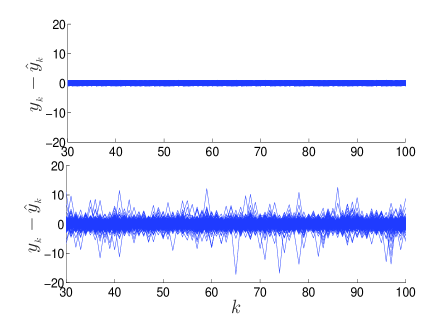
Figure 1: Example 1: Estimation error: (Top) the proposed estimator with $N=6$; (Bottom) MWLSE with $N=6$.

5.2 Example 2: Performance with outlier

An outlier of $-10$ is introduced at $k=30$.

Figure 2 shows 1000 simulation runs of the proposed estimator (Equation (20)) and MWLSE (Equation (22)). The yellow curves are the mean values of the 1000 runs. The proposed estimator is less affected by the outlier than the MWLSE. These yellow curves in the top and bottom figures can be calculated from (29) and (31) respectively.

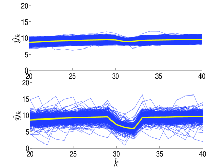
Figure 2: Example 2: (Top) $\hat{y}_{k}$ of the proposed MHE-TD estimator; (Bottom) $\hat{y}_{k}$ of MWLSE.

5.3 Example 3: Comparison with particle filter

The proposed estimator is compared with a particle filter (bootstrap implementation)[3]. Taking the numerical solution of MLE (4) as the ground truth, we compared the estimators using the index

$$I_{k}=\textstyle{\frac{1}{1000}\sum_{j=1}^{1000}\left\|\hat{x}_{k}^{(MLE,j)}-\hat{x}_{k}^{(j)}\right\|_{2}^{2}}$$

where, for the $j$-th run, $\hat{x}_{k}^{(MLE,j)}$ is the numerical solution of the MLE (4) and $\hat{x}_{k}^{(j)}$ is the estimate of $x_{k}$. The indexes, at $k=50$, are $0.0082$, $0.0142$ and $0.0016$ for the proposed estimator, and particle filters with 100 and 1000 particles respectively. The computational times per run using MATLAB R2015a with i7-5500U processor @2.4GHz, 16 GB RAM, are of the order of $0.1$ millisecond, one millisecond and ten milliseconds respectively. For about the same performances ($0.0082$ and $0.0142$) as given by index $I$, the computational time of the proposed estimator is an order of magnitude faster than the particle filter.

6 Conclusion

The IF is employed to give an approximate solution to the moving horizon MLE for ARMAX process with $t$-distribution noise. The approximate solution can be formulated as a recursive MHE-TD algorithm which makes it suitable for on-line and real-time implementation at high sampling rates. We also used the IF to derive a formula for the estimates. The examples show that the proposed estimator gives an estimate with a smaller variance than the MWLSE. It is also less affected by outliers than the MWLSE. For about the same performance index, the computational time of the proposed estimator is an order of magnitude faster than the particle filter.

Appendix A Appendix: Derivation of (10)

Differentiating Equation (8) wrt. $h$ gives

$$\textstyle{\sum_{k=1}^{T}\int_{-\infty}^{\infty}}\frac{d\psi_{k}\left(e_{k}\right)}{dh}\left[(1-h)f\left(e_{k}\right)+h\Delta_{e_{k}}\right]de_{k}$$

$$+\textstyle{\sum_{k=1}^{T}\int_{-\infty}^{\infty}}\psi_{k}\left(e_{k}\right)\left[-f\left(e_{k}\right)+\Delta_{e_{k}}\right]de_{k}=0.$$ (32)

Substituting (7) and

$$\frac{d\psi_{k}\left(e_{k}\right)}{dh}=\frac{d\psi_{k}\left(e_{k}\right)}{d\hat{x}_{1}(h)}\frac{d\hat{x}_{1}(h)}{dh}$$

into (32) gives

$$\textstyle{\sum_{k=1}^{T}\int_{-\infty}^{\infty}}\frac{d\psi_{k}\left(e_{k}\right)}{d\hat{x}_{1}(h)}\left[(1-h)f\left(e_{k}\right)+h\Delta_{e_{k}}\right]de_{k}\frac{d\hat{x}_{1}(h)}{dh}$$

$$+\textstyle{\sum_{k=1}^{T}\int_{-\infty}^{\infty}}\psi_{k}\left(e_{k}\right)\Delta_{e_{k}}de_{k}=0.$$ (33)

Setting $h=0$ in (33) gives

$$\textstyle{\sum_{k=1}^{T}\int_{-\infty}^{\infty}}\frac{d\psi_{k}\left(e_{k}\right)}{d\hat{x}_{1}(h)}f\left(e_{k}\right)de_{k}\left.\frac{d\hat{x}_{1}(h)}{dh}\right|_{h=0}$$

$$+\textstyle{\sum_{k=1}^{T}\int_{-\infty}^{\infty}}\psi_{k}\left(e_{k}\right)\Delta_{e_{k}}de_{k}=0.$$

We denote $\hat{x}_{1}(0)$ as $\bar{x}_{1}$.

Thus we have

$$\left.\frac{d\hat{x}_{1}(h)}{dh}\right|_{h=0} = -\left(\textstyle{\sum_{k=1}^{T}\int_{-\infty}^{\infty}}\frac{d\psi_{k}\left(e_{k}\right)}{d\hat{x}_{1}}f\left(e_{k}\right)de_{k}\right)^{-1}$$ (34)

$$\times\left.\textstyle{\sum_{k=1}^{T}}\psi_{k}\left(e_{k}\right)\right|_{\hat{x}_{1}=\bar{x}_{1}}.$$

Replacing the integration variable $e_{k}$ by $e$ in (34) gives

$$\left.\frac{d\hat{x}_{1}(h)}{dh}\right|_{h=0} = -\left(\textstyle{\sum_{k=1}^{T}\int_{-\infty}^{\infty}}\frac{d\psi_{k}\left(e\right)}{d\hat{x}_{1}}f\left(e\right)de\right)^{-1}$$

$$\times\left.\textstyle{\sum_{k=1}^{T}}\psi_{k}\left(e_{k}\right)\right|_{\hat{x}_{1}=\bar{x}_{1}}.$$

which is (10).

Appendix B Appendix: Proof of Lemma 2

Substituting (2) into (5a)

$$-{\rm ln}f\left(e_{k}\right)$$

$$= -\ln\left(\frac{{\bf\Gamma}\left(\frac{\nu+1}{2}\right)}{\sqrt{\nu\pi}\sigma{\bf\Gamma}\left(\frac{\nu}{2}\right)}\right.$$

$$\left.\times\left(1+\frac{\left(y_{k}-H\Phi^{k-1}\hat{x}_{1}-H{\color[rgb]{0,0,0}s}_{k}\right)^{2}}{\sigma^{2}\nu}\right)^{-\frac{\nu+1}{2}}\right)$$

$$= -{\rm ln}\left(\frac{{\bf\Gamma}\left(\frac{\nu+1}{2}\right)}{\sqrt{\nu\pi}\sigma{\bf\Gamma}\left(\frac{\nu}{2}\right)}\right)$$

$$+\frac{\nu+1}{2}{\rm ln}\left(1+\frac{\left(y_{k}-H\Phi^{k-1}\hat{x}_{1}-H{\color[rgb]{0,0,0}s}_{k}\right)^{2}}{\sigma^{2}\nu}\right).$$

Differentiating $-{\rm ln}f\left(e_{k}\right)$ with respect to $\hat{x}_{1}$ gives

$$\psi_{k}\left(e_{k}\right)=\frac{d}{d\hat{x}_{1}}\left(-{\rm ln}f\left(e_{k}\right)\right)$$ (35)

$$= \frac{\nu+1}{2}\frac{d}{d\hat{x}_{1}}\left({\rm ln}\left(1+\frac{\left(y_{k}-H\Phi^{k-1}\hat{x}_{1}-H{\color[rgb]{0,0,0}s}_{k}\right)^{2}}{\sigma^{2}\nu}\right)\right)$$

$$= -\frac{(\nu+1)\left(H\Phi^{k-1}\right)^{{}^{\prime}}\left(y_{k}-H\Phi^{k-1}\hat{x}_{1}-H{\color[rgb]{0,0,0}s}_{k}\right)}{\sigma^{2}\nu+\left(y_{k}-H\Phi^{k-1}\hat{x}_{1}-H{\color[rgb]{0,0,0}s}_{k}\right)^{2}}$$

$$= -\frac{(\nu+1)\left(H\Phi^{k-1}\right)^{{}^{\prime}}e_{k}}{\sigma^{2}\nu+\left(e_{k}\right)^{2}}.$$

Differentiating $\psi_{k}\left(e\right)$ with respect to $\hat{x}_{1}$ gives

$$\frac{d\psi_{k}\left(e\right)}{d\hat{x}_{1}} = -\frac{d}{d\hat{x}_{1}}\left(\frac{(\nu+1)\left(H\Phi^{k-1}\right)^{{}^{\prime}}e}{\sigma^{2}\nu+e^{2}}\right)$$ (36)

$$= \left(H\Phi^{k-1}\right)^{{}^{\prime}}H\Phi^{k-1}{(\nu+1)\left(\sigma^{2}\nu-e^{2}\right)\over\left(\sigma^{2}\nu+e^{2}\right)^{2}}.$$

Substituting (35) and (36) into (10) gives

$${\rm IF}(e)$$

$$= \left(\textstyle{\sum_{k=1}^{T}\left(H\Phi^{k-1}\right)^{{}^{\prime}}H\Phi^{k-1}\int_{-\infty}^{\infty}}\frac{\left(\nu+1\right)\left(\sigma^{2}\nu-e^{2}\right)}{\left(\sigma^{2}\nu+e^{2}\right)^{2}}f\left(e\right)de\right)^{-1}$$

$$\times\left.\textstyle{\sum_{k=1}^{T}}\frac{\left(\nu+1\right)\left(H\Phi^{k-1}\right)^{{}^{\prime}}e_{k}}{\sigma^{2}\nu+(e_{k})^{2}}\right|_{\hat{x}_{1}=\bar{x}_{1}}$$

which is (11).

When $\nu=\infty$ we have

$$\mathop{\rm lim}_{\nu\rightarrow\infty}\textstyle{\int_{-\infty}^{\infty}}{(\nu+1)\left(\sigma^{2}\nu-e^{2}\right)\over\left(\sigma^{2}\nu+e^{2}\right)^{2}}f(e)de=\frac{1}{\sigma^{2}}$$ (37a)

and

$$\mathop{\rm lim}_{\nu\rightarrow\infty}{\left(\nu+1\right)\left(H\Phi^{k-1}\right)^{{}^{\prime}}e_{k}\over\sigma^{2}\nu+e_{k}^{2}}=\frac{\left(H\Phi^{k-1}\right)^{{}^{\prime}}e_{k}}{\sigma^{2}}.$$ (37b)

Substituting (37a) and (37b) into (11) and setting $e_{k}=y_{k}-H\Phi^{k-1}{\color[rgb]{0,0,0}\bar{x}_{1}}-H{\color[rgb]{0,0,0}s}_{k}$ give

$${\rm IF}(e) = -\bar{x}_{1}+\left(\textstyle{\sum_{k=1}^{T}}\left(H\Phi^{k-1}\right)^{{}^{\prime}}H\Phi^{k-1}\right)^{-1}$$

$$\times\textstyle{\sum_{k=1}^{T}}\left(H\Phi^{k-1}\right)^{{}^{\prime}}\left(y_{k}-H{\color[rgb]{0,0,0}s}_{k}\right)$$

which is (12).

Appendix C Appendix: Proof of Theorem 5

Rewriting the state space model (3) of ARMAX as

$$x_{k+1} = \Phi x_{k}+\Gamma u_{k}+\Omega y_{k}$$ (38)

$$y_{k} = Hx_{k}+e_{k}$$

where $\Phi=\Phi_{a}-\Omega H$. Then using (16) the current state estimate $x_{{}_{T}}$ is obtained by recursively applying the model (38)

$$\hat{x}_{{}_{T}} = \Phi^{T-1}{\rm IF}(e)+\textstyle{\sum_{k=1}^{T-1}}\Phi^{T-k-1}\left(\Gamma u_{k}+\Omega y_{k}\right)$$ (39)

$$= {\color[rgb]{0,0,0}s}_{{}_{T}}+\Phi^{T-1}{\rm{IF}}(e),$$

where $s_{{}_{T}}$ is given by (5d).

Multiplying (17) by $\Phi^{T-1}$ and simplifying give

$$\Phi^{T-1}{\rm IF}(e)$$ (40)

$$= \left(\textstyle{\sum_{\begin{subarray}{c}i=1\end{subarray}}^{N}}\left(H\Phi^{i-N}\right)^{{}^{\prime}}H\Phi^{i-N}\int_{-\infty}^{\infty}{(\nu+1)\left(\sigma^{2}\nu-e^{2}\right)\over\left(\sigma^{2}\nu+e^{2}\right)^{2}}f(e)de\right)^{-1}$$

$$\times\textstyle{\sum_{k=T-N+1}^{T}}{(\nu+1)\left(H\Phi^{k-T}\right)^{{}^{\prime}}\left(y_{k}-H{s}_{k}\right)\over\sigma^{2}\nu+\left(y_{k}-H{s}_{k}\right)^{2}}$$

Rewriting (40) gives

$$\Phi^{T-1}{\rm IF}(e)=\left(\textstyle{\sum_{i=1}^{N}}\left(H\Phi^{i-N}\right)^{\prime}H\Phi^{i-N}\right)^{-1}\varPsi\mathcal{W}_{T,N},$$

(41)

where

$$\varPsi = \left[\begin{matrix}\left(H\Phi^{1-N}\right)^{{}^{\prime}}&\left(H\Phi^{2-N}\right)^{{}^{\prime}}&\cdots&H^{{}^{\prime}}\end{matrix}\right],$$

$$\mathcal{W}_{T,N} = \left[\begin{matrix}w_{{}_{T-N+1}}&w_{{}_{T-N+2}}&\cdots&w_{{}_{T}}\end{matrix}\right]^{{}^{\prime}},$$

$$w_{{}_{T-N+i}} = \left(\textstyle{\int\limits_{-\infty}^{\infty}}\frac{\left(\nu+1\right)\left(\sigma^{2}\nu-e^{2}\right)}{\left(\sigma^{2}\nu+e^{2}\right)^{2}}f(e)de\right)^{-1}$$

$$\times\frac{\left(\nu+1\right)\left(y_{{}_{T-N+i}}-H{\color[rgb]{0,0,0}s}_{{}_{T-N+i}}\right)}{\sigma^{2}\nu+\left(y_{{}_{T-N+i}}-H{\color[rgb]{0,0,0}s}_{{}_{T-N+i}}\right)^{2}},~{}i=1,2,\cdots,N.$$

Equation (18a) is obtained by substituting (41) into (39).

Appendix D Appendix: Proof of Theorem 6

Define

$$\Delta x_{{}_{T}}=\left(\textstyle{\sum_{i=1}^{N}}\left(H\Phi^{i-N}\right)^{\prime}H\Phi^{i-N}\right)^{-1}\varPsi{\mathcal{W}}_{T,N}.$$ (42)

Thus the estimator (18a) can be written as

$$\hat{x}_{{}_{T}}={\color[rgb]{0,0,0}s}_{{}_{T}}+\Delta x_{{}_{T}}.$$

Notice that Equation (42) gives $\Delta x_{{}_{T}}$ from the minimization of the Moving Window Least-Squares loss function

$$V=\frac{1}{2}\textstyle{\sum_{i=1}^{N}}\left(w_{{}_{T-N+i}}-H\Phi^{i-N}\Delta x_{T})\right)^{2}.$$

The recursive solution of the above Moving Window Least-Squares [11] is

$$\Delta x_{{}_{T+1}} = \left(\Phi-L_{N}H\Phi\right)\Delta x_{{}_{T}}+L_{N}w_{{}_{T+1}}$$

$$-\tilde{L}_{N}\left(w_{{}_{T-N+1}}-H\Phi^{-N+1}\Delta x_{{}_{T}}\right),$$

where

$$L_{N} = \Phi^{N-1}P_{N}\left(H\Phi^{N-1}\right)^{{}^{\prime}},$$

$$\tilde{L}_{N} = \Phi^{N-1}P_{N}\left(H\Phi^{-1}\right)^{{}^{\prime}},$$

$$P_{N} = \left(\textstyle{\sum_{i=1}^{N}}\left(H\Phi^{i-1}\right)^{{}^{\prime}}H\Phi^{i-1}\right)^{-1}.$$

In the next time instant

$$\hat{x}_{{}_{T+1}} = {\color[rgb]{0,0,0}s}_{{}_{T+1}}+\Delta x_{{}_{T+1}}$$ (43)

$$= \Phi{\color[rgb]{0,0,0}s}_{{}_{T}}+\Gamma u_{{}_{T}}+\Omega y_{{}_{T}}+\left(\Phi-L_{N}H\Phi\right)\Delta x_{{}_{T}}$$

$$+L_{N}w_{{}_{T+1}}-\tilde{L}_{N}\left(w_{{}_{T-N+1}}-H\Phi^{-N+1}\Delta x_{{}_{T}}\right)$$

$$= \Phi\hat{x}_{{}_{T}}+\Gamma u_{{}_{T}}+\Omega y_{{}_{T}}+L_{N}\left(w_{{}_{T+1}}-H\Phi\Delta x_{{}_{T}}\right)$$

$$-\tilde{L}_{N}\left(w_{{}_{T-N+1}}-H\Phi^{-N+1}\Delta x_{{}_{T}}\right).$$

Expressing (5d) in recursive form we have

$${\color[rgb]{0,0,0}s}_{{}_{T+1}}=\Phi{\color[rgb]{0,0,0}s}_{{}_{T}}+\Gamma u_{{}_{T}}+\Omega y_{{}_{T}}$$ (44)

and

$${\color[rgb]{0,0,0}s}_{{}_{T-N+1}}=\Phi^{-N+1}\left({\color[rgb]{0,0,0}s}_{{}_{T}}-\textstyle{\sum_{i=1}^{N-1}}\Phi^{i-1}\left(\Gamma u_{{}_{T-i}}+\Omega y_{{}_{T-i}}\right)\right).$$

(45)

Define $z_{k}=w_{k}+H{\color[rgb]{0,0,0}s}_{k}.$ Substituting $w_{{}_{T+1}}=z_{{}_{T+1}}-H{\color[rgb]{0,0,0}s}_{{}_{T+1}}$ and $w_{{}_{T-N+1}}=z_{{}_{T-N+1}}-H{\color[rgb]{0,0,0}s}_{{}_{T-N+1}}$ into (43) gives

$$\hat{x}_{{}_{T+1}} = \Phi\hat{x}_{{}_{T}}+\Gamma u_{{}_{T}}+\Omega y_{{}_{T}}$$

$$+L_{N}\left(z_{{}_{T+1}}-H{\color[rgb]{0,0,0}s}_{{}_{T+1}}-H\Phi\Delta x_{{}_{T}}\right)$$

$$-\tilde{L}_{N}\left(z_{{}_{T-N+1}}-H{\color[rgb]{0,0,0}s}_{{}_{T-N+1}}-H\Phi^{-N+1}\Delta x_{{}_{T}}\right).$$

Substituting (44) and (45) into (LABEL:xhatTT1) gives

$$\hat{x}_{{}_{T+1}}$$

$$= \Phi\hat{x}_{{}_{T}}+\Gamma u_{{}_{T}}+\Omega y_{{}_{T}}+L_{N}\left(z_{{}_{T+1}}-H\left(\Phi\hat{x}_{{}_{T}}+\Gamma u_{{}_{T}}+\Omega y_{{}_{T}}\right)\right)$$

$$-\tilde{L}_{N}\left(z_{{}_{T-N+1}}-H\Phi^{-N+1}\hat{x}_{{}_{T}}\right.$$

$$\left.+H\Phi^{-N+1}\left(\varXi_{u}U_{T-1,N-1}+\varXi_{y}Y_{T-1,N-1}\right)\right)$$

which is Equation (20a), and (20b) follows.

Appendix E Appendix: Proof of Theorem 8

By substituting $y_{k}=Hx_{k}+e_{k}$ into (5d) and assuming $x_{1}=0$ for simplicity, $s_{{}_{T}}$ can be rewritten as

$${\color[rgb]{0,0,0}s}_{{}_{T}} = \textstyle{\sum_{k=1}^{T-1}}\Phi_{a}^{T-k-1}\left(\Gamma u_{k}+\Omega e_{k}\right),~{}T\geqslant 2.$$ (47)

Substituting (47) into (39) gives

$$\hat{x}_{{}_{T}}=\textstyle{\sum_{k=1}^{T-1}}{\color[rgb]{0,0,0}\Phi_{a}}^{T-k-1}\left(\Gamma u_{k}+\Omega e_{k}\right)+\Phi^{T-1}{\rm{IF}}(e).$$ (48)

Taking expectation of (48), recognizing that $e_{k}$ is zero mean and $\textstyle{\int_{-\infty}^{\infty}}{\rm{IF}}(e)g(e)de=0$ from (17), we get

$$E\left(\hat{x}_{{}_{T}}\right)=\textstyle{\sum_{k=1}^{T-1}}{\color[rgb]{0,0,0}\Phi_{a}}^{T-k-1}\Gamma u_{k}.$$

Therefore the variance of $\hat{x}_{{}_{T}}$ is given by

$$Var\left(\hat{x}_{{}_{T}}\right) = E\left(\left(\hat{x}_{{}_{T}}-E\left(\hat{x}_{{}_{T}}\right)\right)\left(\hat{x}_{{}_{T}}-E\left(\hat{x}_{{}_{T}}\right)\right)^{{}^{\prime}}\right)$$

$$= \textstyle{\int_{-\infty}^{\infty}}\left(\textstyle{\sum_{k=1}^{T-1}}{\color[rgb]{0,0,0}\Phi_{a}}^{T-k-1}\Omega e_{k}+\Phi^{T-1}{\rm{IF}}(e)\right)$$

$$\times\left(\textstyle{\sum_{k=1}^{T-1}}{\color[rgb]{0,0,0}\Phi_{a}}^{T-k-1}\Omega e_{k}+\Phi^{T-1}{\rm{IF}}(e)\right)^{{}^{\prime}}g(e)de.$$

Substituting (17) into (LABEL:varyhatapp1), noticing that $e_{k}$ is i.i.d and simplifying, give

$$Var\left(\hat{x}_{{}_{T}}\right) = \textstyle{\frac{\rho_{1}}{\rho_{4}^{2}}}M_{N}+2{\color[rgb]{0,0,0}\frac{\rho_{2}}{\rho_{4}}M_{N}}\textstyle{\sum_{i=1}^{N-1}}\left(H\Phi^{i-N}\right)^{{}^{\prime}}\left({\color[rgb]{0,0,0}\Phi_{a}}^{N-i-1}\Omega\right)^{{}^{\prime}}$$

$$+{\color[rgb]{0,0,0}\rho_{3}}\textstyle{\sum_{k=1}^{T-1}}\left({\color[rgb]{0,0,0}\Phi_{a}}^{T-k-1}\Omega\right)\left({\color[rgb]{0,0,0}\Phi_{a}}^{T-k-1}\Omega\right)^{{}^{\prime}},$$

where

$$\rho_{1} = \textstyle{\int_{-\infty}^{\infty}}\left(\frac{(\nu+1)e}{\sigma^{2}\nu+e^{2}}\right)^{2}g(e)de,~{}\rho_{2}=\textstyle{\int_{-\infty}^{\infty}}\frac{(\nu+1)e^{2}}{\sigma^{2}\nu+e^{2}}g(e)de,$$

$$\rho_{3} = \textstyle{\int_{-\infty}^{\infty}}e^{2}g(e)de,~{}\rho_{4}=\textstyle{\int_{-\infty}^{\infty}}{(\nu+1)\left(\sigma^{2}\nu-e^{2}\right)\over(\sigma^{2}\nu+e^{2})^{2}}g(e)de,$$

$$M_{N} = \left(\textstyle{\sum_{i=1}^{N}}\left(H\Phi^{i-N}\right)^{{}^{\prime}}H\Phi^{i-N}\right)^{-1},$$ (50)

which is (23), and (24) follows.

Appendix F Appendix: Proof of Theorem 10

Recall (47) and $x_{1}=0$

$${s}_{{}_{T}} = \textstyle{\sum_{k=1}^{T-1}}{\Phi_{a}}^{T-k-1}\left(\Gamma u_{k}+\Omega e_{k}\right).$$

Then

$$E\left({s}_{{}_{T}}\right)=\left\{\begin{aligned} &\textstyle{\sum_{k=1}^{T-1}}{\Phi_{a}}^{T-k-1}\Gamma u_{k}~{}~{}~{}~{}~{}~{}~{}~{}~{}~{}~{}~{}{\rm if}~{}T\leq k_{1},\\ &\textstyle{\sum_{k=1}^{T-1}}{\Phi_{a}}^{T-k-1}\Gamma u_{k}+{\Phi_{a}}^{T-k_{1}-1}\Omega e_{k_{1}}\\ &~{}~{}~{}~{}~{}~{}~{}~{}~{}~{}~{}~{}~{}~{}~{}~{}~{}~{}~{}~{}~{}~{}~{}~{}~{}~{}~{}~{}~{}~{}~{}~{}~{}~{}~{}~{}~{}~{}~{}~{}{\rm if}~{}T>k_{1},\end{aligned}\right.$$

which is (10). Let $k_{2}=k_{1}+N-1$.

Substituting (50) into (40) gives

$$\Phi^{T-1}{\rm IF}(e) = M_{N}\left(\int_{-\infty}^{\infty}{(\nu+1)\left(\sigma^{2}\nu-e^{2}\right)\over\left(\sigma^{2}\nu+e^{2}\right)^{2}}f(e)de\right)^{-1}$$ (51)

$$\times\textstyle{\sum_{k=T-N+1}^{T}}{(\nu+1)\left(H\Phi^{k-T}\right)^{{}^{\prime}}\left(y_{k}-H{s}_{k}\right)\over\sigma^{2}\nu+\left(y_{k}-H{s}_{k}\right)^{2}}$$

From the estimator (39) we have

$$E\left(\hat{x}_{{}_{T}}\right) = E\left({s}_{{}_{T}}\right)+\textstyle{\int_{-\infty}^{\infty}}\Phi^{T-1}{\rm IF}(e)g(e)de.$$ (52)

Using (52) and (18b) gives

$$E\left(\hat{y}_{{}_{T}}\right) = HE\left({s}_{{}_{T}}\right)+H\textstyle{\int_{-\infty}^{\infty}}\Phi^{T-1}{\rm{IF}}(e)g_{k}(e)de.$$ (53)

Substituting (51) and (28) into the second term of (53) and simplifying give

$$H\textstyle{\int_{-\infty}^{\infty}}\Phi^{T-1}{\rm{IF}}(e)g_{k}(e)de$$

$$= \left\{\begin{aligned} &HM_{N}\left(\textstyle{\int_{-\infty}^{\infty}}\frac{\left(\nu+1\right)\left(\sigma^{2}\nu-e^{2}\right)}{\left(\sigma^{2}\nu+e^{2}\right)^{2}}f(e)de\right)^{-1}\\ &~{}~{}~{}\times\textstyle{\int_{-\infty}^{\infty}}{\frac{\left(\nu+1\right)\left(H\Phi^{k_{1}-T}\right)^{{}^{\prime}}e}{\sigma^{2}\nu+e^{2}}\Delta_{e_{k_{1}}}de}\\ &~{}~{}~{}{+}HM_{N}\left(\textstyle{\int_{-\infty}^{\infty}}\frac{\left(\nu+1\right)\left(\sigma^{2}\nu-e^{2}\right)}{\left(\sigma^{2}\nu+e^{2}\right)^{2}}f(e)de\right)^{-1}\\ &~{}~{}~{}\textstyle{\int_{-\infty}^{\infty}\sum_{\begin{subarray}{c}i=1\\ i\neq{k_{1}-T+N}\end{subarray}}^{N}}\frac{\left(\nu+1\right)\left(H\Phi^{i-{N}}\right)^{{}^{\prime}}e}{\sigma^{2}\nu+e^{2}}g(e)de\\ &~{}~{}~{}~{}~{}~{}~{}~{}~{}~{}~{}~{}~{}~{}~{}~{}~{}~{}~{}~{}~{}~{}~{}~{}~{}~{}~{}~{}~{}~{}~{}~{}~{}~{}~{}~{}~{}~{}~{}~{}~{}~{}~{}~{}~{}~{}{\rm if}~{}k_{1}\leq T\leq k_{2},\\ &\\ &0~{}~{}~{}~{}~{}~{}~{}~{}~{}~{}~{}~{}~{}~{}~{}~{}~{}~{}~{}~{}~{}~{}~{}~{}~{}~{}~{}~{}~{}~{}~{}~{}~{}~{}~{}~{}~{}~{}{\rm if}~{}T<k_{1}~{}{\rm or}~{}T>k_{2}.\end{aligned}\right.$$

With

$$\textstyle{\int_{-\infty}^{\infty}\sum_{\begin{subarray}{c}i=1\\ i\neq k_{1}-T+N\end{subarray}}^{N}}\frac{\left(\nu+1\right)\left(H\Phi^{{i}-N}\right)^{{}^{\prime}}e}{\sigma^{2}\nu+e^{2}}g_{k}(e)de=0,$$

equation (LABEL:intIF2) becomes

$$H\textstyle{\int_{-\infty}^{\infty}}\Phi^{T-1}{\rm{IF}}(e)g(e)de$$

$$= \left\{\begin{aligned} &HM_{N}\left(\textstyle{\int_{-\infty}^{\infty}}\frac{\left(\nu+1\right)\left(\sigma^{2}\nu-e^{2}\right)}{\left(\sigma^{2}\nu+e^{2}\right)^{2}}f(e)de\right)^{-1}\\ &~{}~{}~{}\textstyle{\int_{-\infty}^{\infty}}{\frac{\left(\nu+1\right)\left(H\Phi^{k_{1}-T}\right)^{{}^{\prime}}e}{\sigma^{2}\nu+e^{2}}\Delta_{e_{k_{1}}}de}~{}~{}~{}{\rm if}~{}k_{1}\leq T\leq k_{2},\\ &\\ &0~{}~{}~{}~{}~{}~{}~{}~{}~{}~{}~{}~{}~{}~{}~{}~{}~{}~{}~{}~{}~{}~{}~{}~{}~{}~{}~{}~{}~{}~{}~{}~{}~{}~{}~{}~{}~{}~{}{\rm if}~{}T<k_{1}~{}{\rm or}~{}T>k_{2},\end{aligned}\right.$$

$$= \left\{\begin{aligned} &\textstyle{\frac{1}{\rho_{4}}}HM_{N}\frac{\left(H\Phi^{k_{1}-T}\right)^{{}^{\prime}}(\nu+1)e_{k_{1}}}{\sigma^{2}\nu+e_{k_{1}}^{2}}~{}~{}~{}~{}~{}~{}~{}~{}~{}{\rm if}~{}k_{1}\leq T\leq k_{2},\\ &0~{}~{}~{}~{}~{}~{}~{}~{}~{}~{}~{}~{}~{}~{}~{}~{}~{}~{}~{}~{}~{}~{}~{}~{}~{}~{}~{}~{}~{}~{}~{}~{}~{}~{}~{}~{}~{}~{}{\rm if}~{}T<k_{1}~{}{\rm or}~{}T>k_{2}.\end{aligned}\right.$$

Equation (29) is obtained by substituting (LABEL:intIF3) into (53).

Appendix G Appendix: Numerical Illustration Example

For example, for $N=6$ and $k=9$, substituting the parameters for Example 1 into (24) gives

$$M_{N} = \left(\sum_{i=1}^{6}\left(\left[\begin{matrix}1&0&0&&0&0\end{matrix}\right]\left[\begin{matrix}-4.0000&1&0&0&0\\ -6.4000&0&1&0&0\\ -5.1200&0&0&1&0\\ -2.0480&0&0&0&1\\ -0.3278&0&0&0&0\end{matrix}\right]^{i-6}\right)^{{}^{\prime}}\right.$$

$$\left.\times\left[\begin{matrix}1&0&0&&0&0\end{matrix}\right]\left[\begin{matrix}-4.0000&1&0&0&0\\ -6.4000&0&1&0&0\\ -5.1200&0&0&1&0\\ -2.0480&0&0&0&1\\ -0.3277&0&0&0&0\end{matrix}\right]^{i-6}\right)^{-1}$$

$$= \left[\begin{matrix}0.9887&0.7858&0.3986&0.1163&0.0148\\ 0.7858&16.8432&16.2135&6.6997&1.0672\\ 0.3986&16.2135&16.4601&7.0558&1.1553\\ 0.1163&6.6997&7.0558&3.1051&0.5187\\ 0.0148&1.0672&1.1553&0.5187&0.0880\end{matrix}\right]$$

and

$$Var\left(\hat{y}_{{}_{T}}\right)=0.9887\frac{\rho_{1}}{\rho_{4}^{2}}+0.0064\frac{\rho_{2}}{\rho_{4}}+0.4481\rho_{3}=0.7055,$$

$\rho_{1}=2.6667,~{}\rho_{2}=1,~{}\rho_{3}=0.7414,~{}\rho_{4}=2.6667$. Substituting the parameters for Example 1 into (LABEL:varyhatgaussian) gives

$$Var\left(\hat{y}_{{}_{T}}\right)=\rho_{3}\left(0.9887+0.0064+0.4481\right)=1.0705.$$

References

- [1] Gabriel Agamennoni, Juan I Nieto, and Eduardo M Nebot. Approximate inference in state-space models with heavy-tailed noise. Signal Processing, IEEE Transactions on, 60(10):5024–5037, 2012.
- [2] Gabriel Agamennoni, Juan I Nieto, and Eduardo Mario Nebot. An outlier-robust Kalman filter. In Robotics and Automation (ICRA), 2011 IEEE International Conference on, pages 1551–1558. IEEE, 2011.
- [3] M Sanjeev Arulampalam, Simon Maskell, Neil Gordon, and Tim Clapp. A tutorial on particle filters for online nonlinear/non-Gaussian Bayesian tracking. Signal Processing, IEEE Transactions on, 50(2):174–188, 2002.
- [4] Karl Johan Åström and Björn Wittenmark. Computer-controlled systems: theory and design. Courier Dover Publications, 2011.
- [5] Luisa Turrin Fernholz. On multivariate higher order von mises expansions. Metrika, 53(2):123–140, 2001.
- [6] Frank R Hampel, Elvezio M Ronchetti, Peter J Rousseeuw, and Werner A Stahel. Robust statistics: the approach based on influence functions, volume 114. John Wiley & Sons, 2011.
- [7] Weng Khuen Ho, Keck Voon Ling, Hoang Dung Vu, and Xiaoqiong Wang. Filtering of the ARMAX process with generalized t-distribution noise: The influence function approach. Industrial Engineering Chemistry Research, 53(17):7019–7028, 2014.
- [8] Peter J Huber. Robust statistics. John Wiley & Sons, 1981.
- [9] Peter J Huber et al. Robust estimation of a location parameter. The Annals of Mathematical Statistics, 35(1):73–101, 1964.
- [10] Samuel Kotz and Saralees Nadarajah. Multivariate t-distributions and their applications. Cambridge University Press, 2004.
- [11] KV Ling and KW Lim. Receding horizon recursive state estimation. Automatic Control, IEEE Transactions on, 44(9):1750–1753, 1999.
- [12] Ricardo Maronna, Doug Martin, and Victor Yohai. Robust Statistics: Theory and Methods. John Wiley & Sons, Chichester. ISBN, 2006.
- [13] R J Meinhold and Nozer D Singpurwalla. Robustification of Kalman filter models. Journal of the American Statistical Association, 84(406):479–486, 1989.
- [14] R V Mises. On the asymptotic distribution of differentiable statistical functions. The annals of mathematical statistics, 18(3):309–348, 1947.
- [15] Michael Roth, Emre Ozkan, and Fredrik Gustafsson. A student’s t filter for heavy tailed process and measurement noise. In Acoustics, Speech and Signal Processing (ICASSP), 2013 IEEE International Conference on, pages 5770–5774. IEEE, 2013.
- [16] D Wang and JA Romagnoli. A framework for robust data reconciliation based on a generalized objective function. Industrial engineering chemistry research, 42(13):3075–3084, 2003.