Scheme-Independent Calculations of Physical Quantities in an ${\cal N}=1$ Supersymmetric Gauge Theory

Abstract

We consider an asymptotically free, vectorial, ${\cal N}=1$ supersymmetric gauge theory with gauge group $G$ and $N_{f}$ pairs of chiral superfields in the respective representations ${\cal R}$ and $\bar{\cal R}$ of $G$, having an infrared fixed point (IRFP) of the renormalization group at $\alpha_{IR}$. We present exact results for the anomalous dimensions of various (gauge-invariant) composite chiral superfields $\gamma_{{\Phi}_{\rm prod}}$ at the IRFP and prove that these increase monotonically with decreasing $N_{f}$ in the non-Abelian Coulomb phase of the theory and that scheme-independent expansions for these anomalous dimensions as powers of an $N_{f}$-dependent variable, $\Delta_{f}$, exhibit monotonic and rapid convergence to the exact $\gamma_{{\Phi}_{\rm prod}}$ throughout this phase. We also present a scheme-independent calculation of the derivative of the beta function, $d\beta/d\alpha|_{\alpha=\alpha_{IR}}$, denoted $\beta^{\prime}_{IR}$, up to $O(\Delta_{f}^{3})$ for general $G$ and ${\cal R}$, and, for the case $G={\rm SU}(N_{c})$, ${\cal R}=F$, we give an analysis of the properties of $\beta^{\prime}_{IR}$ calculated to $O(\Delta_{f}^{4})$.

I Introduction

An important fact about quantum field theories is that their properties depend on the Euclidean energy/momentum scale $\mu$ at which these properties are measured. The change in these properties as a function of $\mu$ is described by the renormalization group (RG). Asymptotically free gauge theories are particularly amenable to renormalization-group analysis because the running gauge coupling, $g(\mu)$, goes to zero in the limit of large $\mu$ in the deep ultraviolet (UV), so that in this regime one can describe the theory accurately using perturbative methods. The dependence of $g(\mu)$, or equivalently, $\alpha(\mu)=g(\mu)^{2}/(4\pi)$, on $\mu$, is described by the beta function,

$$\beta=\frac{d\alpha}{dt}\ ,$$ (1)

where $dt=d\ln\mu$.

Here we consider an asymptotically free, vectorial, ${\cal N}=1$ supersymmetric gauge theory with gauge group $G$ and $N_{f}$ pairs of massless chiral superfields $\Phi_{i}$ and $\tilde{\Phi}_{i}$ transforming according to the respective representations ${\cal R}$ and $\bar{\cal R}$ of $G$ fm . In an asymptotically free theory of this type, as $\mu$ decreases from large values in the UV toward $\mu=0$ in the infrared, $\alpha(\mu)$ increases. There are several possible types of infrared behavior, depending on the gauge group and matter content of the theory. We focus on the case in which the beta function has a zero at a certain value $\alpha=\alpha_{IR}$, which is an IR fixed point (IRFP) of the renormalization group. Thus, as $\mu$ decreases from the UV to the IR, $\alpha(\mu)$ increases (monotonically) from 0 to the limiting value $\alpha_{IR}$. In this IR limit, the theory is scale-invariant, and is inferred to be conformally invariant scalecon . The combination of this conformal invariance with the supersymmetry means that the theory is invariant under a superconformal algebra. We denote the full operator dimension of a physical (gauge-invariant) operator ${\cal O}$ as $D_{\cal O}$. In general, this can be written as

$$D_{\cal O}=D_{{\cal O},{\rm free}}-\gamma_{\cal O}\ ,$$ (2)

where $D_{{\cal O},{\rm free}}$ is the Maxwellian dimension that the operator would have in a free theory and $\gamma_{\cal O}$ is the anomalous dimension of ${\cal O}$ anomdimconv .

In this paper we present new scheme-independent results on the values of physical quantities at this superconformal IR fixed point. These quantities include anomalous dimensions of gauge-invariant operators, $\gamma_{\cal O}$ and the derivative of the beta function, $\beta^{\prime}\equiv d\beta/d\alpha$, evaluated at $\alpha=\alpha_{IR}$ and thus denoted $\gamma_{{\cal O},IR}$ and $\beta^{\prime}_{IR}$. Specifically, we present exact results for anomalous dimensions of various (gauge-invariant) composite chiral superfield operator products $\Phi_{\rm prod}$ and study the properties of scheme-independent expansions of these operators as power series in $\Delta_{f}$, where $\Delta_{f}$ is an $N_{f}$-dependent expansion variable given in Eq. (37) below. bz ; gk ; gg . We prove that these anomalous dimensions increase monotonically with decreasing $N_{f}$ in the non-Abelian Coulomb phase of the theory and that scheme-independent expansions for these anomalous dimensions as powers of $\Delta_{f}$ exhibit monotonic and rapid convergence to the exact $\gamma_{{\Phi}_{\rm prod}}$ throughout this phase. We also present a scheme-independent calculation of $\beta^{\prime}_{IR}$ up to $O(\Delta_{f}^{3})$ for general $G$ and ${\cal R}$ and analyze the properties of this expansion up to $O(\Delta_{f}^{4})$ for $G={\rm SU}(N_{c})$ and ${\cal R}=F$, the fundamental representation. Previously, we have presented results for the anomalous dimension $\gamma_{M,IR}$ of a meson-type chiral superfield using $n$-loop series expansions and scheme-independent series expansions bfs -ir . The current paper substantially extends our earlier results.

This paper is organized as follows. Some relevant background and methods are discussed in Section II. In Section III we prove several theorems on anomalous dimensions of (gauge-invariant) chiral superfields. In Sections IV-VI we present exact results on anomalous dimensions of various composite chiral superfield operators. These are generalized to theories with higher-dimension matter chiral superfields in Section VII. Section VIII contains our results on $\beta^{\prime}_{IR}$. For the case $G={\rm SU}(N_{c})$ and ${\cal R}=F$, Section IX contains an analysis of properties in the limit $N_{c}\to\infty$ and $N_{f}\to\infty$ with the ratio $N_{f}/N_{c}$ fixed and finite. Our conclusions are given in Section X.

II Background and Methods

In this section we review some background and methods that we will use in our calculations. We consider an asymptotically free ${\cal N}=1$ supersymmetric vectorial gauge theory with gauge group $G$ and $N_{f}$ copies (flavors) of matter chiral superfields $\Phi^{i}$ and $\tilde{\Phi}_{i}$, $1\leq i\leq N_{f}$, transforming as the ${\cal R}$ and $\bar{\cal R}$ representations of $G$, respectively. We write the decomposition of the matter chiral superfield $\Phi$ in terms of component fields (with group and flavor indices suppressed here) as

$$\Phi=\phi+\sqrt{2}\,\theta\psi+\theta\theta F\ ,$$ (3)

where $\phi$, $\psi$, and $F$ are, respectively, the scalar, fermionic, and auxiliary component fields, and $\theta$ is an anticommuting Grassmann variable. The chiral superfield $W_{\alpha}$ contains the gluino $\lambda_{\alpha}$ and the field-strength tensor $F_{\mu\nu}^{a}$, where here $\alpha$ and $a$ are spinor and gauge indices, respectively.

The beta function of this theory has the series expansion

$$\beta=-2\alpha\sum_{\ell=1}^{\infty}b_{\ell}\,\Big{(}\frac{\alpha}{4\pi}\Big{)}^{\ell}=-2\alpha\sum_{\ell=1}^{\infty}\bar{b}_{\ell}\,\alpha^{\ell}\ ,$$ (4)

where $b_{\ell}$ is the $\ell$-loop coefficient and $\bar{b}_{\ell}=b_{\ell}/(4\pi)^{\ell}$. The first two coefficients, which are scheme-independent gross75 , are jones75 ; casimir

$$b_{1}=3C_{A}-2T_{f}N_{f}$$ (5)

and susyloops

$$b_{2}=6C_{A}^{2}-4(C_{A}+2C_{f})T_{f}N_{f}\ .$$ (6)

The requirement of asymptotic freedom restricts $N_{f}$ to be less than an upper ($u$) bound $N_{u}$, i.e.,

$$N_{f}<N_{u}\ ,$$ (7)

where

$$N_{u}=\frac{3C_{A}}{2T_{f}}\ .$$ (8)

Note that $N_{u}$ is not necessarily an integer nfintegral .

The anomalous dimension of a (gauge-invariant) operator ${\cal O}$ has a series expansion in powers of the coupling of the form

$$\gamma_{\cal O}=\sum_{\ell=1}^{\infty}c_{{\cal O},\ell}\,\Big{(}\frac{\alpha}{4\pi}\Big{)}^{\ell}\ ,$$ (9)

where $c_{{\cal O},\ell}$ is the $\ell$-loop coefficient. In particular, for a chiral superfield $\Phi$, one may write

$$\gamma_{\Phi}=\sum_{\ell=1}^{\infty}c_{\ell}\,\Big{(}\frac{\alpha}{4\pi}\Big{)}^{\ell}\ .$$ (10)

From a calculation of the contribution of instantons to the action, Novikov, Shifman, Vainshtein, and Zakharov (NSVZ) derived a closed-form expression for the beta function nsvz :

$$\beta_{NSVZ}=-\frac{\alpha^{2}}{2\pi}\bigg{[}\frac{b_{1}-2N_{f}T_{f}\,\gamma_{M}}{1-\frac{C_{A}\alpha}{2\pi}}\bigg{]}\ ,$$ (11)

where $\gamma_{M}$ is the anomalous dimension of the fermion bilinear that occurs in the (gauge-invariant) quadratic chiral superfield operator product. We focus here on the IR non-Abelian Coulomb phase (NACP), to be discussed further below, in which the nonanomalous global chiral symmetry of the theory is exact. Although we will analyze meson and baryon operators, as well as other gauge-invariant products of chiral superfields later in the paper, it should be kept in mind that there is no confinement in this NACP, and hence no physical mesons or baryons. The reason that we restrict to gauge-singlet operators is so that the corresponding anomalous dimensions are gauge-invariant and hence physical.

In the NACP, a quadratic chiral superfield operator transforms according to an (irreducible) representation of this global chiral symmetry. Since the anomalous dimensions are the same for these different representations (see, e.g., gracey_gammatensor ), we denote the common anomalous dimension simply as that for the singlet representation, corresponding to the quadratic operator product $\tilde{\Phi}\Phi=\sum_{i=1}^{N_{f}}\tilde{\Phi}_{i}\Phi^{i}$. Since this corresponds to the (gauge-invariant) fermion bilinear $\bar{\psi}\psi$ in a non-supersymmetric vectorial gauge theory, the anomalous dimension $\gamma_{M}$ has often been denoted as $\gamma_{\bar{\psi}\psi}$ in our previous papers bfs ; gtr ; gsi ; dex ; dexs ; dexl .

A number of exact results have been established about the (zero-temperature) IR phase structure of the theory nsvz ; seiberg ; susyreviews . In the IR limit $\mu\to 0$, $\alpha(\mu)$ approaches the limiting value $\alpha_{IR}$. In particular, the theory flows from the UV to a non-Abelian Coulomb phase (NACP) in the IR if

$${\rm NACP}:\quad N_{\ell}<N_{f}<N_{u}\ ,$$ (12)

where

$$N_{\ell}=\frac{3C_{A}}{4T_{f}}=\frac{N_{u}}{2}\ .$$ (13)

As with $N_{u}$, note that $N_{\ell}$ is not necessarily an integer; it is the actual physical lower end of the NACP if and only if it is an integer. In particular, we note the important special case

$$G={\rm SU}(N_{c}),\ \ {\cal R}=F\ \Longrightarrow\ N_{\ell}=\frac{3}{2}N_{c},\ \ N_{u}=3N_{c},$$ (14)

(15)

(16)

so that in this special case, $N_{\ell}$ is only physical if and only if $N_{c}$ is even. This is to be understood implicitly below, when $N_{\ell}$ is referred to as the lower end of the non-Abelian Coulomb phase nellphysical . Throughout the paper we will often consider a formal generalization in which $N_{f}$ is analytically continued from the non-negative integers to the (non-negative) real numbers, with the understanding that physical values of $N_{f}$ are positive integers. One reason for doing this is to study the behavior of various quantities as $N_{f}$ approaches $N_{u}$ from below and $N_{\ell}$ from above in the non-Abelian phase.

The two-loop beta function has an IR zero if $N_{f}$ is in the interval $N_{f,b2z}<N_{f}<N_{u}$, where

$$N_{f,b2z}=\frac{3C_{A}^{2}}{2T_{f}(C_{A}+2C_{f})}\ .$$ (17)

As we discussed in bfs , $N_{f,b2z}$ may be larger than or smaller than $N_{\ell}$, depending on the chiral superfield representation ${\cal R}$. One has

$$N_{f,b2z}-N_{\ell}=\frac{3C_{A}(C_{A}-2C_{f})}{4T_{f}(C_{A}+2C_{f})}\ .$$ (18)

This difference can be positive or negative. For the fundamental representation, ${\cal R}=F$,

$${\cal R}=F\ \Longrightarrow\ N_{f,b2z}-N_{\ell}=\frac{3N_{c}}{2(2N_{c}^{2}-1)}\ ,$$ (19)

which is positive. However, for example, for the adjoint representation, $R=adj$, this difference is negative:

$${\cal R}=adj:\ \Longrightarrow\ N_{f,b2z}-N_{\ell}=-\frac{1}{4}\ .$$ (20)

For general $G$, the supersymmetric theory under consideration here is invariant under a classical continuous global ($gb$) symmetry

$$G_{cgb} = {\rm U}(N_{f})\otimes{\rm U}(N_{f})\otimes{\rm U}(1)_{R}$$ (21)

$$= {\rm SU}(N_{f})\otimes{\rm SU}(N_{f})\otimes{\rm U}(1)_{V}\otimes{\rm U}(1)_{A}\otimes{\rm U}(1)_{R}\ ,$$ (23)

where the first and second U($N_{f}$) groups consist of operators acting on $\Phi=(\Phi^{1},...,\Phi^{N_{f}})$ and $\tilde{\Phi}=(\tilde{\Phi}_{1},...,\tilde{\Phi}_{N_{f}})$, respectively, and the U(1)_R group is defined by the commutation relations

$$[Q_{\alpha},R]=Q_{\alpha}\ ,\quad[Q_{\alpha}^{\dagger},R]=-Q_{\alpha}^{\dagger}\ ,$$ (26)

where the $Q_{\alpha}$ and $Q_{\alpha}^{\dagger}$ are the generators of the supersymmetry transformations (with $\alpha$ a spinor index here). The U(1)_A symmetry is anomalous, due to instantons, so the actual nonanomalous continuous global symmetry of the theory is

$$G_{gb}={\rm SU}(N_{f})\otimes{\rm SU}(N_{f})\otimes{\rm U}(1)_{V}\otimes{\rm U}(1)_{R}\ .$$ (27)

This symmetry is exact at a superconformal IRFP in the non-Abelian Coulomb phase. Usually, for a U(1) (global or gauge) symmetry, the physics is invariant under a multiplication of the charges of all fields by a nonzero real constant. However, the situation is different for the U(1)_R symmetry in a superconformal field theory; in this case, the $R$ charges of chiral superfields under the (global) U(1)_R symmetry are uniquely determined susyreviews ; mack ; dim_rcharge_rel ; susyreviews2 ; intriligator_wecht .

The representations of the matter chiral superfields under the gauge and global symmetry groups are listed in Table 1 for the generic case in which the representation ${\cal R}$ is complex. The case of (real) ${\cal R}$ will be discussed below.) We recall the derivation of the $R$-charge assignment to $\Phi$ and $\tilde{\Phi}$ (noting also that one can take $R_{\Phi}=R_{\tilde{\Phi}}$). This assignment can be determined by the condition that the U(1)_R symmetry should not have a triangle anomaly determines the $R$ charges of $\Phi$ (where the gauge and flavor indices are suppressed in the notation). The $R$ charge of the fermionic component $\psi$ in $\Phi$ is $R_{\psi}=R_{\Phi}-1$. Given that $R_{\lambda}=1$ for the gluino, $\lambda$, the sum of the contributions to the triangle anomaly from the gluino, and the $\Phi$ and $\tilde{\Phi}$ matter superfields are $C_{A}+2(R_{\Phi}-1)T_{f}N_{f}$. The condition that this sum must be zero yields

$$R_{\Phi}=R_{\tilde{\Phi}}=1-\frac{C_{A}}{2T_{f}N_{f}}\ .$$ (28)

For the U(1)_R symmetry to be non-anomalous, it is also necessary that, similarly to the situation in non-supersymmetric theories, the one-loop contribution is not modified by higher-order contributions, and this requisite property holds susyanomaly .

One can construct gauge-invariant quadratic operator products of the “meson”-type, namely

$$M_{i}^{j}=\tilde{\Phi}_{i}\Phi^{j}\ ,$$ (29)

where, as above, $i$ and $j$ are flavor indices and the group indices are implicit, with it being understood that they are contracted in such a way as to yield a singlet under the gauge group $G$. As a holomorphic product of chiral superfields, $M_{i}^{j}$ is again a chiral superfield. The fermionic bilinear operator product in $M_{i}^{j}$ is $\tilde{\psi}_{i}\psi^{j}\equiv\tilde{\psi}_{i,L}^{T}C\psi^{j}_{L}$, where $C$ is the conjugation Dirac matrix and we follow the usual convention of writing the holomorphic chiral superfields as left-handed. Because the global symmetry (27) is exact in the NACP, the meson-type quadratic chiral superfields transform according to (irreducible) representations of the group $G_{gb}$. We focus on the anomalous dimension of the diagonal operator $\tilde{\Phi}\Phi=\sum_{i=1}^{N_{f}}\tilde{\Phi}_{i}\Phi^{i}$ evaluated at the IRFP $\alpha_{IR}$, which we denote as $\gamma_{M}$.

Consider next the case where $G={\rm SU}(N_{c})$ and ${\cal R}=F$. The transformation properties of the matter chiral superfields in this theory under the global symmetry group $G_{gb}$ are listed in Table 2. Since we focus on the non-Abelian Coulomb NACP, where an IRFP is exact, $N_{f}$ must lie in the interval $(3/2)N_{c}<N_{f}<3N_{c}$. Therefore, $N_{f}$ automatically satisfies the requirement $N_{f}\geq N_{c}$ to construct the baryonic composite chiral superfield operator

$$B^{i_{1}...i_{N_{c}}}=\epsilon_{a_{1}\ldots a_{N_{c}}}\Phi^{a_{1},i_{1}}\Phi^{a_{2},i_{2}}\cdots\Phi^{a_{N_{c}},i_{N_{c}}}$$ (30)

and the corresponding operator involving the $\tilde{\Phi}$ chiral superfields,

$$\tilde{B}_{i_{1}...i_{N_{c}}}=\epsilon_{a_{1}\ldots a_{N_{c}}}\tilde{\Phi}_{i_{1}}^{a_{1}}\tilde{\Phi}_{i_{2}}^{a_{2}}\cdots\tilde{\Phi}_{i_{N_{c}}}^{a_{N_{c}}}\ ,$$ (31)

where here the $a_{k}$ and the $i_{\ell}$ are group and flavor indices, respectively and $\epsilon_{a_{1}\ldots a_{N_{c}}}$ is the totally antisymmetric tensor density for the SU($N_{c}$) gauge group. (If $N_{f}<N_{c}$, the operator products (30) and (31) vanish identically.). Since the flavors are equivalent with respect to the gauge interaction, we will henceforth suppress the flavor dependence in the notation. The full scaling dimensions of $\Phi$ and $\tilde{\Phi}$ are equal, and the same is true for the full scaling dimensions of $B$ and $\tilde{B}$, i.e., $D_{B,F}=D_{{\tilde{B}},F}$ (where the subscript indicates that ${\cal R}=F$, the fundamental representation), so that the anomalous dimensions of these baryonic operators, denoted $\gamma_{B,F}$ and $\gamma_{{\tilde{B}},F}$, are also equal. We thus have

$$D_{B,F}=D_{{\tilde{B}},F} = D_{B,F,{\rm free}}-\gamma_{B,F}$$ (32)

$$= N_{c}-\gamma_{B,F}\ .$$ (34)

We shall discuss baryonic chiral superfield operator products for the case where ${\cal R}$ is a higher-dimensional representation of $G$ later in the paper.

In general (suppressing flavor indices), from $M$, $B$, and $\tilde{B}$, one can construct a number of different composite gauge-invariant chiral superfields. We denote such a generic composite chiral superfield consisting of a (holomorphic) product of $n_{M}$ factors of a meson-type chiral superfield $M$ times $n_{B}$ factors of $B$ and $n_{\tilde{B}}$ factors of $\tilde{B}$ chiral superfields as $\Phi_{\rm prod}$:

$$\Phi_{\rm prod}=M^{n_{M}}B^{n_{B}}\tilde{B}^{n_{\tilde{B}}}\ .$$ (35)

Here, to avoid cumbersome notation, the values of $n_{M}$, $n_{B}$, and $n_{\tilde{B}}$ are kept implicit in $\Phi_{\rm prod}\equiv\Phi_{{\rm prod};n_{M},n_{B},n_{\tilde{B}}}$. One could also include a factor $(W_{\alpha}W^{\alpha})^{n_{W}}$, but (35) will be sufficient for our present analysis.

There are several important quantities that characterize the properties of the superconformal field theory at the IRFP at $\alpha_{IR}$. These include the derivative

$$\beta^{\prime}_{IR}\equiv\frac{d\beta}{d\alpha}\bigg{|}_{\alpha=\alpha_{IR}}$$ (36)

and the anomalous dimensions of various gauge-invariant composite chiral superfield operators evaluated at $\alpha=\alpha_{IR}$ such as $\gamma_{M}$, $\gamma_{B}$, $\gamma_{{\tilde{B}}}$, and $\gamma_{\Phi_{\rm prod}}$. (Here and below, we will often leave the dependence on ${\cal R}$ implicit in the notation.)

As (gauge-invariant) physical quantities, $\beta^{\prime}_{IR}$ and these anomalous dimensions are scheme-independent. However, the series expansions of these quantities in powers of $\alpha$, calculated to a finite order, do not maintain this scheme-independence beyond the lowest orders. Hence, it is quite useful to calculate and analyze series expansions for these quantities that are scheme-independent at each order. An important property is that $\alpha_{IR}\searrow 0$ as $N_{f}\nearrow N_{u}$. This property is also shared by a quantity that is manifestly scheme-independent, namely

$$\Delta_{f}=N_{u}-N_{f}\ ,$$ (37)

where $N_{u}$ was defined in Eq. (8). The maximal value of $\Delta_{f}$ in the NACP is

$$(\Delta_{f})_{max,NACP}=N_{u}-N_{\ell}=\frac{N_{u}}{2}=\frac{3C_{A}}{4T_{f}}\ .$$ (38)

As was observed by Banks and Zaks bz (for a non-supersymmetric vectorial gauge theory, in which $N_{u}=11C_{A}/(4T_{f})$), $\Delta_{f}$ is a natural scheme-independent expansion variable. In addition to bz , some early work with the $\Delta_{f}$ expansion was carried out in gk ; gg . In addition to our previous works on scheme-independent series expansions gtr ; gsi ; dex ; dexs ; dexl , see also kataev .

One may write a scheme-independent series expansions of $\beta^{\prime}_{IR}$ in powers of $\Delta_{f}$ as

$$\beta^{\prime}_{IR}=\sum_{j=2}^{\infty}d_{j}\,\Delta_{f}^{j}\ .$$ (39)

In general, the calculation of $d_{j}$ requires, as inputs, the values of $b_{\ell}$ with $1\leq\ell\leq j$.

The property that $d_{1}=0$, so that $\beta^{\prime}_{IR}$ vanishes like $\Delta_{f}^{2}$ as $\Delta_{f}\to 0$, was derived in dex . This property is general and does not depend on whether the theory is supersymmetric or non-supersymmetric. A simple way to understand this result is to note that for either type of theory, the one-loop coefficient in the beta function has the form $b_{1}=b_{1,0}+b_{1,1}N_{f}$ (where $b_{1,0}>0$ and $b_{1,1}<0$), so that $N_{u}=-b_{1,0}/b_{1,1}$. Then, since $\Delta_{f}=N_{u}-N_{f}=-b_{1}/b_{1,1}$, it follows that

$$\Delta_{f}\propto b_{1}\ .$$ (40)

From Eq. (123) below, $\beta^{\prime}_{IR}=-2a_{IR}\sum_{\ell=1}^{\infty}(\ell+1)b_{\ell}\,a_{IR}^{\ell-1}$, where $a_{IR}=\alpha_{IR}/(4\pi)$. As $N_{f}\to N_{u}$, $\alpha_{IR}$ vanishes linearly in $\Delta_{f}$, so in this limit, $\beta^{\prime}_{IR}\propto\alpha_{IR}b_{1}\propto\Delta_{f}^{2}$.

One may write the scheme-independent series expansion of $\gamma_{M}$ at the superconformal IRFP in powers of $\Delta_{f}$ for a meson superfield operator:

$$\gamma_{M}=\sum_{j=1}^{\infty}\kappa_{j}\,\Delta_{f}^{j}\ .$$ (41)

The calculation of $\kappa_{j}$ requires, as inputs, the values of $b_{\ell}$ with $1\leq\ell\leq j+1$ and $c_{\ell}$ with $1\leq\ell\leq j$. Similarly, the scheme-independent series expansion of $\gamma_{B}=\gamma_{\tilde{B},IR}$ at the IRFP in powers of $\Delta_{f}$ can be written as

$$\gamma_{B}=\gamma_{\tilde{B}}=\sum_{j=2}^{\infty}f_{B,j}\Delta_{f}^{j}\ .$$ (42)

More generally, the scheme-independent expansion for a gauge-invariant composite chiral superfield $\Phi_{\rm prod}$ consisting of a (holomorphic) product of an arbitrary number of mesonic, baryonic, and conjugate baryonic superfields, evaluated at the IRFP, can be written as

$$\gamma_{\Phi_{\rm prod}}=\sum_{j=2}^{\infty}f_{\Phi_{\rm prod},j}\Delta_{f}^{j}\ .$$ (43)

These are thus series expansions extending downward below $N_{u}$ in the non-Abelian Coulomb phase. The truncations of these infinite series to order $j=p$ inclusive are denoted $\beta^{\prime}_{IR,\Delta_{f}^{p}}\equiv\beta^{\prime}_{\Delta_{f}^{p}}$, $\gamma_{M,\Delta_{f}^{p}}$, $\gamma_{B,\Delta_{f}^{p}}$, and $\gamma_{\Phi_{\rm prod},\Delta_{f}^{p}}$, respectively.

For a scalar operator (other than the identity), the condition of unitarity in a conformal field theory implies the lower bound mack ; dim_rcharge_rel ; gir

$$D_{\cal O}\geq 1\ .$$ (44)

This bound holds regardless of whether the theory is supersymmetric or not.

In a supersymmetric conformal (i.e., superconformal) theory, one can take advantage of additional information about the operator dimensions. First, if a (composite or fundamental) chiral superfield ${\cal O}$ has $R$ charge $R_{\cal O}$, then susyreviews ; mack ; dim_rcharge_rel ; susyreviews2 ; gir ; minwalla

$$D_{\cal O}=\frac{3}{2}\,R_{\cal O}\ .$$ (45)

We recall that since $D_{\cal O}$ is a physical quantity, the meaningfulness of this relation depends on the fact that in a superconformal theory, the $R$ charges are uniquely determined. Since the U(1)_R symmetry is exact in the non-Abelian Coulomb phase considered here, the $R$ charge of an operator is a conserved quantity. The $R$ charge of a holomorphic product of chiral superfields is the sum of the $R$ charges of each of the chiral superfields in the product:

$$R_{\Phi_{\rm prod}}=\sum_{k=1}^{p}R_{\Phi_{k}}\ .$$ (46)

Hence, the full dimension of a holomorphic product $\Phi_{\rm prod}$ of chiral superfields $\Phi_{k}$, $k=1,...,p$, $\Phi_{\rm prod}=\prod_{k=1}^{p}\Phi_{k}$, is the sum of the full dimensions of each chiral superfield in the product (e.g., susyreviews2 ):

$$D_{\Phi_{\rm prod}}=\sum_{k=1}^{p}D_{\Phi_{k}}\ .$$ (47)

Furthermore, the anomalous dimension of $\Phi_{\rm prod}$ is the sum of the anomalous dimensions of the individual $\Phi_{k}$ superfields:

$$\gamma_{\Phi_{\rm prod}}=\sum_{k=1}^{p}\gamma_{\Phi_{k}}\ .$$ (48)

III Theorems on Properties of the Anomalous Dimensions of Composite Chiral Superfields

In this section we prove some theorems on the properties of anomalous dimension $\gamma_{\Phi_{\rm prod}}$ of a gauge-invariant composite chiral superfield consisting of a (holomorphic) product of powers of $\Phi$ and/or $\tilde{\Phi}$ (where flavor indices are suppressed). Our results for the anomalous dimensions $\gamma_{\Phi_{\rm prod}}$ of various particular composite chiral superfields given later in the paper will illustrate these general theorems.

The properties of the $R$ charge (28) form the basis of the resultant properties of the anomalous dimensions of the various composite chiral superfields that we will consider. We first use these properties to prove a general monotonicity theorem concerning the anomalous dimension of a chiral superfield operator containing products of $\Phi$ and/or $\tilde{\Phi}$. This theorem applies for an arbitrary gauge group $G$ and fermion representation. We recall that $N_{\ell}=N_{u}/2$, as is evident in Eqs. (8) and (13). For the following discussion, we implicitly use the above-mentioned generalization of $N_{f}$ from non-negative integers to real numbers. As $N_{f}$ decreases from $N_{u}$ to $N_{\ell}$ in the NACP, $R_{\Phi}$ decreases from 0 to $-1$. Since the full scaling dimension of a chiral superfield operator containing products of $\Phi$ and/or $\tilde{\Phi}$ satisfies (45) and since this full dimension is related to the anomalous dimension of the operator according to (2), it follows that the anomalous dimension $\gamma_{\cal O}$ is a monotonically increasing function of decreasing $N_{f}$ in the NACP, which increases from $\gamma_{\cal O}=0$ at the upper end of the NACP to a maximal value at the lower end of the NACP.

We next prove a theorem on the structure the anomalous dimension of a general composite chiral superfield containing products of $\Phi$ and/or $\tilde{\Phi}$, and the coefficients $f_{\Phi_{\rm prod},j}$ in (43). To do this, we first express $R_{\Phi}=R_{\tilde{\Phi}}$ as a function of $\Delta_{f}$, obtaining

$$R_{\Phi}=1-\frac{1}{1-\frac{\Delta_{f}}{N_{u}}}\ .$$ (49)

Combining this with Eqs. (45) and (2), it follows, as a second theorem, that the anomalous dimension of a general composite chiral superfield containing products of $\Phi$ and/or $\tilde{\Phi}$, evaluated at the superconformal IRFP, is of the form

$$\gamma_{\Phi_{prod}} = C\Big{[}1-\frac{1}{1-\frac{\Delta_{f}}{N_{u}}}\Big{]}$$ (50)

$$= C\sum_{j=1}^{\infty}\Big{(}\frac{\Delta_{f}}{N_{u}}\Big{)}^{j}\ ,$$ (52)

where $C$ is a $\Delta_{f}$-independent constant depending on $G$, the fermion representation, and the structure of $\Phi_{prod}$. Hence, as a corollary to this theorem, we find that the coefficient $f_{\Phi_{\rm prod},j}$ of the $O(\Delta_{f}^{j})$ term in the expansion (43) is given by

$$f_{\Phi_{\rm prod},j}=\frac{1}{N_{u}^{j}}\ .$$ (53)

That is, up to an overall multiplicative factor $C$, $\gamma_{\Phi_{\rm prod}}$ is a geometric series in powers of $\Delta_{f}$, with the coefficients given in Eq. (53). As is evident in Eq. (53) is positive, this coefficient $f_{\Phi_{\rm prod},j}$ is positive. This leads to two further monotonicity theorems. Define $\gamma_{\Phi_{rmprod},\Delta_{f}^{p}}$ as equal to the right-hand side of Eq. (43) with the upper limit $j=\infty$ replaced by $j=p$, i.e., the truncation of this infinite series to order $O(\Delta_{f}^{p})$. Then the positivity of the coefficients $f_{\Phi_{\rm prod},j}$ implies, as the third and fourth theorems, that (i) for fixed $p$, the $O(\Delta_{f}^{p})$ approximation, $\gamma_{\Phi_{rmprod},\Delta_{f}^{p}}$, to the exact $\gamma_{\Phi_{\rm prod}}$, is a monotonically increasing function of $\Delta_{f}$, i.e., of decreasing $N_{f}$, and (ii) for fixed $N_{f}$ and thus $\Delta_{f}$, $\gamma_{\Phi_{rmprod},\Delta_{f}^{p}}$ is a monotonically increasing function of the truncation order, $p$. We had noted these monotonicity results in our earlier work for $\gamma_{M}$ gtr ; gsi ; dex ; dexs ; dexl , and here we prove them in general.

A fifth theorem concerns the region of analyticity of the expression for $\gamma_{\Phi_{prod}}$ in (52) and the corresponding radius of convergence of the series expansion (43) in powers of $\Delta_{f}$. As is evident in Eq. (52), this exact explicit expression for $\gamma_{\Phi_{prod}}$ is an analytic function of $\Delta_{f}$ in the complex $\Delta_{f}$ plane within a disk defined by

$$|\Delta_{f}|<N_{u}$$ (54)

and, correspondingly, the infinite series (43) converges for all $\Delta_{f}$ in this disk. This region of convergence covers the entire non-Abelian Coulomb phase because the maximal value of $\Delta_{f}$ in this phase, as given by Eq. (38), is $(\Delta_{f})_{max,NACP}=N_{u}/2$.

IV Anomalous Dimension $\gamma_{M}$

In this section we discuss some results on $\gamma_{M}$ at a superconformal IRFP that will be used in the paper. Since

$$R_{M}=R_{\Phi}+R_{\tilde{\Phi}}=2\Big{(}1-\frac{C_{A}}{2T_{f}N_{f}}\Big{)}\ ,$$ (55)

the full dimension of the quadratic chiral superfield operator $M$ (at the superconformal IRFP) is

$$D_{M} = \frac{3}{2}R_{M}=3\Big{(}1-\frac{C_{A}}{2T_{f}N_{f}}\Big{)}$$ (56)

$$= 2-\gamma_{M}\ ,$$ (58)

and hence

$$\gamma_{M}=\frac{3C_{A}}{2T_{f}N_{f}}-1=\frac{N_{u}}{N_{f}}-1\ .$$ (59)

where $N_{u}$ depends on ${\cal R}$. Expressing this anomalous dimension in terms of $\Delta_{f}$, we have

$$\gamma_{M}=\frac{1}{1-\frac{\Delta_{f}}{N_{u}}}-1=\sum_{j=1}^{\infty}\bigg{(}\frac{\Delta_{f}}{N_{u}}\bigg{)}^{j}\ ,$$ (60)

so the coefficient $\kappa_{j}$ in Eq. (41) is

$$\kappa_{j}=\frac{1}{N_{u}^{j}}=\Big{(}\frac{2T_{f}}{3C_{A}}\Big{)}^{j}\ .$$ (61)

One sees that this general derivation is consistent with the NSVZ beta function. This can be seen from the fact that at the IRFP, $\beta_{NSVZ}=0$; solving this equation yields the result (59). Expressing $\gamma_{M}$ as a function of $\Delta_{f}$, we obtain the same results as in Eqs. (60) and (61).

For an ${\cal N}=1$ supersymmetric gauge theories with general $G$ and ${\cal R}$, $\gamma_{M}$ was calculated up to three-loop order in bfs and studied further in bc -bfs2 . Concerning the scheme-independent series expansion (41), for general $G$ and ${\cal R}$, $\kappa_{1}$ and $\kappa_{2}$ were calculated in gtr , while for $G={\rm SU}(N_{c})$ and ${\cal R}=F$, $\kappa_{3}$ was computed in dexs . These calculations used the beta function coefficients $b_{1}$-$b_{4}$ and the anomalous dimension coefficients $c_{1}$-$c_{3}$ from jones75 ; susyloops ; susyloops2 . Importantly, we found that the results of our scheme-independent calculations of the $\kappa_{j}$ for this supersymmetric gauge theory agreed perfectly with the Taylor series expansion of the exact expression (60).

Furthermore, as is evident from the exact result (60), the small-$\Delta_{f}$ expansion of the exact result is (absolutely) convergent for $|\Delta_{f}|<N_{u}$, i.e.,

$$|\Delta_{f}|<\frac{3C_{A}}{2T_{f}}\ .$$ (62)

This covers all of the non-Abelian Coulomb phase, which extends from $N_{u}=3C_{A}/(2T_{f})$ down to $N_{\ell}=N_{u}/2=3C_{A}/(4T_{f})$, i.e., from $\Delta_{f}=0$ to $\Delta_{f}=3C_{A}/(4T_{f})$.

We next discuss the limiting values of $\gamma_{M}$ at a superconformal IRFP at the upper and lower end of the NACP. If one formally generalizes $N_{f}$ from the positive integers to real numbers and lets $N_{f}$ decrease from $N_{u}$ to $N_{\ell}$ in the NACP, $\gamma_{M}$ increases monotonically from 0 to 1, saturating the upper bound allowed by conformal invariance at the lower end of the NACP. This behavior holds for general matter chiral superfield representation $R$ and is a consequence of the fact that $N_{\ell}=N_{u}/2$. As stated, this is formal, because, in general, neither $N_{u}$ nor $N_{\ell}$ is an integer, so the physical $N_{f}$, restricted as it is to integer values, cannot necessarily take on either the value $N_{u}$ at which $\gamma_{M}=0$ or the value $N_{\ell}$ at which $\gamma_{M}\nearrow 1$, saturating the upper bound from conformality. In order for $N_{f}$ to be able to reach $N_{\ell}$, it is necessary that $N_{\ell}$ be an integer. In the case $G={\rm SU}(N_{c})$ with ${\cal R}=F$, (i) $N_{u}$ is always an integer, but (ii) since $N_{\ell}=(3/2)N_{c}$, it follows that $N_{\ell}$ is an integer if and only if $N_{c}$ is even. If, on the other hand, $N_{c}$ is odd, then as $N_{c}$ decreases from $N_{u}=3N_{c}$ in the NACP, it cannot actually reach $N_{\ell}$ since the latter is half-integral. In this case, $\gamma_{M}$ does not saturate its conformality upper bound at the lower end of the NACP. In this case where the matter chiral superfield representation is ${\cal R}=F$, one may avoid this complication by taking the limit $N_{c}\to\infty$, $N_{f}\to\infty$ with the ratio $r=N_{f}/N_{c}$ fixed and finite. As will be discussed below, in this limit, $r$ is a real number and can always reach the lower end of the non-Abelian Coulomb phase, so that $\gamma_{M}$ always saturates its upper bound from conformal invariance.

It should be noted that the $\Delta_{f}$ expansion avoids a problem in which an IRFP may not be manifest as a physical IR zero of the $n$-loop beta function for some $n$. Indeed, although the two-loop beta function, $\beta_{2\ell}$, and the three-loop $\beta_{3\ell}$, calculated in the $\overline{DR}$ scheme, have physical $\alpha_{IR,n\ell}$ zeros for $N_{f,b2z}<N_{f}<N_{u}$ in this supersymmetric theory bfs , we find that the four-loop beta function, $\beta_{4\ell}$ (calculated in the $\overline{DR}$ scheme), does not exhibit a physical IR zero, $\alpha_{IR,4\ell}$, for a substantial range of $N_{f}$ in this interval. This is similar to what we found for $\alpha_{IR,5\ell}$ in the non-supersymmetric gauge theory flir . In both cases, the $\Delta_{f}$ expansions (41) and (39) circumvent this problem of a possible unphysical $\alpha_{IR,n\ell}$ that one may encounter in using the conventional expansions (4).

V Anomalous Dimension $\gamma_{B}=\gamma_{{\tilde{B}}}$ for ${\cal R}=F$

In this section we specialize to the theory with gauge group $G={\rm SU}(N_{c})$ and $N_{f}$ pairs of chiral superfields $\Phi^{a,i}$ and $\tilde{\Phi}_{i}^{a}$ (where $a$ and $j$ are group and flavor indices) in the fundamental and conjugate fundamental representations, denoted $F$ and $\bar{F}$, with Young tableaux       and $\overline{\raisebox{-0.5pt}{\hbox{\rule{0.4pt}{6.5pt}\hskip-0.4pt\rule{6.5pt}{0.4pt}\hskip-6.5pt\rule[6.5pt]{6.5pt}{0.4pt}}\rule[6.5pt]{0.4pt}{0.4pt}\hskip-0.4pt\rule{0.4pt}{6.5pt}}}$, respectively. The matter content of this theory is summarized in Table 2

The $R$ charges of the basic chiral superfields are given in Table 2. From Eq. (46), it follows that

$$R_{B,F}=R_{{\tilde{B}},F}=N_{c}R_{\Phi}=N_{c}\Big{(}1-\frac{N_{c}}{N_{f}}\Big{)}\ .$$ (63)

Combining this with Eq. (45), one has the known exact result

$$D_{B,F}=D_{{\tilde{B}},F}=\frac{3}{2}R_{B,F}=\frac{3}{2}N_{c}\Big{(}1-\frac{N_{c}}{N_{f}}\Big{)}\ .$$ (64)

where we indicate ${\cal R}=F$ explicitly. Hence, the (equal) anomalous dimensions of $B$ and $\tilde{B}$ at the superconformal IRFP are

$$\gamma_{B,F}=\gamma_{{\tilde{B}},F}=\frac{N_{c}}{2}\Big{(}\frac{3N_{c}}{N_{f}}-1\Big{)}\ .$$ (65)

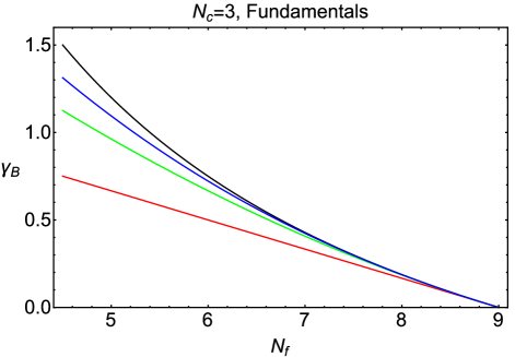
Figure 1: Plot of $\gamma_{B,F,\Delta_{f}^{p}}$ = $\gamma_{\tilde{B},F,\Delta_{f}^{p}}$ with $1\leq p\leq 3$, together with the exact $\gamma_{B,F}$, for $G={\rm SU}(3)$ and ${\cal R}=F$, as a function of $N_{f}$, at an IRFP in the non-Abelian Coulomb phase for this theory. In this and the later figures, we consider $N_{f}$ to be generalized from integers in the NACP to real numbers nfintegral . For notational simplicity, the vertical axis is labeled simply as $\gamma_{B}$. At $N_{f}=8$, from bottom to top, the curves (with colors online) refer to $\gamma_{B,F,\Delta}$ (red), $\gamma_{B,F,\Delta_{f}^{2}}$ (green), $\gamma_{B,F,\Delta_{f}^{3}}$ (blue), and the exact $\gamma_{B,F}$ (black).

In Fig. 1 we plot the the value of $\gamma_{B,F}$ at the IRFP calculated to order $O(\Delta_{f}^{p})$ with $1\leq p\leq 3$, in comparison with the exact value, Eq. (65), for the illustrative value $N_{c}=3$. As was true of $\gamma_{M}$, we see that these $O(\Delta_{f}^{p})$ truncations of the infinite series converge rapidly to the exact result.

Expressed as a function of $\Delta_{f}=3N_{c}-N_{f}$, $\gamma_{B,F}$ is

$$\gamma_{B,F}=\gamma_{{\tilde{B}},F}=\frac{N_{c}}{2}\,\bigg{(}\frac{\frac{\Delta_{f}}{3N_{c}}}{1-\frac{\Delta_{f}}{3N_{c}}}\bigg{)}\ .$$ (66)

From Eqs. (60) and (65), one sees that $\gamma_{B,F}$ is simply proportional to $\gamma_{M,F}$:

$$\gamma_{B,F}=\frac{N_{c}}{2}\,\gamma_{M,F}\ .$$ (67)

As $N_{f}\nearrow 3N_{c}$, i.e., $\Delta_{f}\searrow 0$, the common anomalous dimension $\gamma_{B,F}=\gamma_{{\tilde{B}},F}$ vanishes, and as $N_{f}\searrow(3/2)N_{c}$, i.e., $\Delta_{f}\nearrow(3/2)N_{c}$, it approaches the value

$$\lim_{N_{f}\searrow(3/2)N_{c}}\gamma_{(B,\tilde{B})}=\frac{N_{c}}{2}$$ (68)

from below.

These baryonic composite chiral superfields have spin 0 (and are not equal to the identity), so their respective full dimensions are bounded by the unitarity constraint from conformality, $D_{B}\geq 1$ and $D_{\tilde{B}}\geq 1$. This implies the upper bounds

$$\gamma_{B,F}\leq N_{c}-1\ ,$$ (69)

and thus also $\gamma_{{\tilde{B}},F}\leq N_{c}-1$. Except for the case $N_{c}=2$, where, owing to the reality of the representations of SU(2), the baryonic and mesonic composite chiral superfield operators are equivalent, the anomalous dimensions of the $B$ and $\tilde{B}$ operators at the IRFP do not saturate their unitarity upper bound. This is true, in particular, for the infinite set of even values of $N_{c}$, for which $N_{\ell}$ is an integer and hence is physical. This behavior is in contrast to the situation that we found for the anomalous dimension $\gamma_{M,F}$, which does saturate its upper bound of 1 as $N_{f}\searrow N_{\ell}$ (assuming that $N_{c}$ is even so that $N_{\ell}$ is an integer).

VI Anomalous Dimensions of Composite Chiral Superfields

In this section we derive exact expressions for the full dimension and hence also the anomalous dimension of a variety of composite chiral superfields. We first discuss a SU($N_{c}$) theory with $N_{f}$ pairs of matter chiral superfields $\Phi^{i}$ and $\tilde{\Phi}_{i}$, $i=1,...,N_{f}$, transforming as the $F$ and $\bar{F}$ representations, respectively. Our explicit results illustrate the general theorems that we have proven above concerning these anomalous dimensions. We consider the composite chiral superfield $\Phi_{\rm prod}$ in Eq. (35). Using Eqs. (46), we have

$$R_{\Phi_{\rm prod}}=\Big{[}2n_{M}+(n_{B}+n_{\tilde{B}})N_{c}\Big{]}\Big{(}1-\frac{N_{c}}{N_{f}}\Big{)}\ .$$ (70)

Using Eq. (45), we have

$$D_{\Phi_{\rm prod}}=\frac{3}{2}\Big{[}2n_{M}+(n_{B}+n_{\tilde{B}})N_{c}\Big{]}\Big{(}1-\frac{N_{c}}{N_{f}}\Big{)}\ .$$ (71)

Hence,

$$\gamma_{\Phi_{\rm prod}}=\Big{[}n_{M}+\frac{(n_{B}+n_{\tilde{B}})}{2}\,N_{c}\Big{]}\Big{(}\frac{3N_{c}}{N_{f}}-1\Big{)}\ .$$ (72)

One sees that for the special case $(n_{M},n_{B},n_{\tilde{B}})=(1,0,0)$, the general result (72) reduces to Eq. (59), while for the special cases $(n_{M},n_{B},n_{\tilde{B}})=(0,1,0)$ and $(n_{M},n_{B},n_{\tilde{B}})=(0,0,1)$, Eq. (72) reduces to Eq. (65). Expressing Eq. (72) as a function of $\Delta_{f}$ yields the result

$$\gamma_{\Phi_{\rm prod}} = \Big{[}n_{M}+\frac{(n_{B}+n_{\tilde{B}})}{2}\,N_{c}\Big{]}\bigg{[}\frac{1}{1-\frac{\Delta_{f}}{3N_{c}}}-1\bigg{]}$$ (73)

$$= \Big{[}n_{M}+\frac{(n_{B}+n_{\tilde{B}})}{2}\,N_{c}\Big{]}\,\sum_{j=1}^{\infty}\Big{(}\frac{\Delta_{f}}{3N_{c}}\Big{)}^{j}\ .$$ (75)

In agreement with our general monotonicity theorem proved above, this anomalous dimension $\gamma_{\Phi_{\rm prod}}$ increases monotonically as a function of $\Delta_{f}$ or equivalently decreasing $N_{f}$ in the NACP. As $N_{f}$ decreases below $N_{u}$, $\gamma_{\Phi_{\rm prod}}$ increases monotonically from 0 to a maximum of

$$\lim_{N_{f}\searrow(3/2)N_{c}}\gamma_{\Phi_{\rm prod}}=n_{M}+\Big{(}\frac{n_{B}+n_{\tilde{B}}}{2}\Big{)}N_{c}\ .$$ (78)

From the conformality lower bound on the full dimension, $D_{\Phi_{\rm prod}}\geq 1$, one obtains the corresponding upper bound

$$\gamma_{\Phi_{\rm prod}}\leq 2n_{M}+(n_{B}+n_{\tilde{B}})N_{c}-1\ .$$ (79)

Expanding the exact expression in Taylor series, we read off the coefficient $f_{\Phi_{\rm prod},j}$ as

$$f_{\Phi_{\rm prod},j}=\Big{[}n_{M}+\frac{(n_{B}+n_{\tilde{B}})}{2}\,N_{c}\Big{]}\,\Big{(}\frac{1}{3N_{c}}\Big{)}^{j}\ .$$ (80)

As is evident from Eq. (LABEL:gamma_phiprod_Delta), this series converges if

$$|\Delta_{f}|<3N_{c}\ .$$ (81)

This includes all of the NACP for this theory.

VII Baryonic Operators with Chiral Superfields in Higher-Dimensional Representations

VII.1 General

Here we derive corresponding exact results for anomalous dimensions of (gauge-invariant) composite chiral superfield operators in (a vectorial, asymptotically free, ${\cal N}=1$ supersymmetric) SU($N_{c}$) gauge theory containing $N_{f}$ pairs of matter chiral superfields transforming according to respective higher-dimensional representations ${\cal R}$ and $\bar{\cal R}$ of the gauge group. As part of our analysis, we consider cases in which the representation is real (or pseudoreal), i.e., ${\cal R}=\bar{\cal R}$. For a given type of higher-dimensional representation ${\cal R}$, the value of $N_{f}$ is subject to the constraints that (i) the theory is asymptotically free, so $N_{f}<N_{u}$, where $N_{u}$ was given in Eq. (8), and $N_{f}\geq N_{\ell}$, where $N_{\ell}$ was given in Eq. (13), since we focus here on an exact IRFP in the non-Abelian Coulomb phase.

For a general representation ${\cal R}$ of the matter chiral superfield, the representations (charges) under the (anomaly-free) global symmetry can be read from Table 1. If the gauge representation is real or pseudoreal, then the global symmetry is enhanced, and the matter chiral superfield has the representations given in Table 3. Real representations include the (i) all representations of SU(2), (ii) the adjoint representation of a general group $G$, and (iii) the antisymmetric rank-$k$ representation of SU($2k$).

VII.2 Adjoint Representation

If ${\cal R}$ is the adjoint representation, then $N_{u}=3/2$ and $N_{\ell}=3/4$, which allows just one Dirac value of $N_{f}$, namely $N_{f}=1$. Since the adjoint representation is real, this is equivalent to $N_{f}=2$ Majorana chiral superfields. Furthermore, owing to the reality of the adjoint representation, composite superfields of baryon and meson type are equivalent. We denote these by $M_{i}^{j}$, and they are written as

$$M_{ij}=\Phi^{a_{1}}_{\phantom{a_{1}}a_{2},i}\Phi^{a_{2}}_{\phantom{a_{2}}a_{1}j}=\text{Tr}(\Phi_{i}\Phi_{j})\ ,$$ (82)

where the trace is over color indices, and $i,j$ are flavor indices. The full scaling dimension of this operator is

$$D_{M,adj}=\frac{3}{2}R_{M}=3\Big{(}1-\frac{1}{2N_{f}}\Big{)}\ ,$$ (83)

and therefore the anomalous dimension is

$$\gamma_{M,adj}=2-3\Big{(}1-\frac{1}{2N_{f}}\Big{)}=\frac{3}{2N_{f}}-1\ .$$ (84)

Thus, $\gamma_{M,adj}$ takes the values 1/2 and $-1/4$ for the cases $N_{f}=1,\ 2$, respectively. Note that these values are independent of $N_{c}$. Expressed as a function of $\Delta_{f}=N_{u}-N_{f}=(3/2)-N_{f}$, this anomalous dimension is

$$\gamma_{M,adj}=\frac{1}{1-\frac{2}{3}\Delta_{f}}-1=\sum_{j=1}^{\infty}\Big{(}\frac{2\Delta_{f}}{3}\Big{)}^{j}\ .$$ (85)

We thus identify the coefficient $\kappa_{j}$ for this case as

$$\kappa_{j,adj}=\Big{(}\frac{2}{3}\Big{)}^{j}\ .$$ (86)

As before, formally continuing $N_{f}$ from its allowed integral values to real values, we may study the properties of the small-$\Delta_{f}$ expansion to the exact result. In Fig. 3 we plot $O(\Delta_{f}^{p})$ approximations to $\gamma_{M,adj}$, together with the exact result. As is evident from this figure and from Eq. (84), finite truncations of this series converge rapidly to the exact result in the NACP. As we will see, this rapid convergence is also true of the other anomalous dimensions that we calculate below.

VII.3 Rank-2 Symmetric Tensor Representation

Here we consider the case in which $G={\rm SU}(N_{c})$ and ${\cal R}=S_{2}$, the rank-2 symmetric tensor representation. If $N_{c}=2$, then the $S_{2}$ representation is the adjoint representation, which we have already discussed. Therefore, we take $N_{c}\geq 3$. Here,

$$N_{u,S_{2}}=\frac{3N_{c}}{N_{c}+2}$$ (87)

and

$$N_{\ell,S_{2}}=\frac{3N_{c}}{2(N_{c}+2)}\ ,$$ (88)

so that the non-Abelian Coulomb phase is comprised of the integer values of $N_{f}$ in the formal interval $N_{\ell}\leq N_{f}<N_{u}$, i.e.,

$${\rm NACP}_{S_{2}}:\quad\frac{3N_{c}}{2(N_{c}+2)}\leq N_{f}<\frac{3N_{c}}{N_{c}+2}\ .$$ (89)

The condition that $N_{f}$ should be in the NACP restricts $N_{f}$. For example, for the values $N_{c}=3$ and $N_{c}=4$ the inequality (89) reads $9/10<N_{f}<9/5$ and $1\leq N_{f}<2$, respectively, allowing only the integer value $N_{f}=1$. For $N_{c}=5$, the inequality (106) reads $15/14<N_{f}<15/7$, allowing only the integer value $N_{f}=2$, and more generally, for $N_{c}\geq 5$, the inequality (89) only allows the value $N_{f}=2$. As $N_{c}\to\infty$, the inequality (89) approaches the limiting form $3/2<N_{f}<3$, with only the solution $N_{f}=2$.

For $N_{c}\geq 3$, the $S_{2}$ representation is complex, so we consider both meson and baryon chiral superfield operator products. The meson product is

$$M_{i}^{j}=\tilde{\Phi}_{a_{1}a_{2},i}\Phi^{a_{1}a_{2},j}=\text{Tr}(\tilde{\Phi}_{i}\Phi^{j})\ ,$$ (90)

where the trace is over the color indices and $\Phi^{a_{1}a_{2},i}=\Phi^{a_{2}a_{1},i}$. The full scaling dimension of this operator is

$$D_{M,S_{2}}=\frac{3}{2}R_{M,S_{2}}=3\Big{[}1-\frac{N_{c}}{N_{f}(N_{c}+2)}\Big{]}\ ,$$ (91)

and the anomalous dimension is

$$\gamma_{M,S_{2}} = 2-3\Big{[}1-\frac{N_{c}}{N_{f}(N_{c}+2)}\Big{]}$$ (92)

$$= \frac{3N_{c}}{N_{f}(N_{c}+2)}-1=\frac{N_{u,S_{2}}}{N_{f}}-1\ .$$ (94)

As is clear from Eq. (94), this is of the form (59) with $N_{u}=N_{n,S_{2}}$. Expressed in terms of $\Delta_{f}=N_{u}-N_{f}$, one obtains the special case of (60) for the present theory with $N_{u}=N_{u,S_{2}}$ given by (87). As was the case with ${\cal R}=F$, since $N_{\ell}$ is not, in general, an integer, $N_{f}$ cannot actually decrease all the way to be equal to $N_{\ell}$, so $\gamma_{M,S_{2}}$ does not actually saturate its upper bound $\gamma_{M,S_{2}}\leq 1$ from conformal invariance. However, if one formally analytically continues $N_{f}$ from integers to real numbers, then this $N_{f}$ can decrease all the way to $N_{\ell}$ at the lower boundary of the NACP, so $\gamma_{M,S_{2}}$ does saturate this upper bound. In Fig. 4 we plot $O(\Delta_{f}^{p})$ approximations to $\gamma_{M,S_{2}}$, together with the exact result, for the case $N_{c}=3$. We see again that finite truncations of this series converge rapidly to the exact result throughout the NACP.

The baryon and antibaryon operators in this case are

$$B^{i_{1},\ldots,i_{N_{c}}}=\frac{1}{N_{c}!}\epsilon_{a_{1},\ldots,a_{N_{c}}}\epsilon\ _{a^{\prime}_{1},\ldots,a^{\prime}_{N_{c}}}\Phi^{a_{1}a^{\prime}_{1},i_{1}}\cdots\Phi^{a_{N_{c}}a^{\prime}_{N_{c}},i_{N_{c}\ }}$$ (95)

and

$$\tilde{B}_{i_{1},\ldots,i_{N_{c}}}=\frac{1}{N_{c}!}\epsilon^{a_{1},\ldots,a_{N_{c}}}\ \epsilon^{a^{\prime}_{1},\ldots,a^{\prime}_{N_{c}}}\tilde{\Phi}_{a_{1}a^{\prime}_{1},i_{1}}\cdots\tilde{\Phi}_{a_{N_{c}}a^{\prime}_{N_{c}},i_{N_{c}}}\ .$$ (96)

The way in which the color indices are contracted is similar to the determinant of a matrix. This is the reason we have included the $1/(N_{c}!)$ normalization factor. These operators have $R$ charge

$$R_{B,S_{2}}=R_{{\tilde{B}},S_{2}}=N_{c}\Big{[}1-\frac{N_{c}}{N_{f}(N_{c}+2)}\Big{]}\ .$$ (97)

Hence, the full scaling dimensions of these operators are

$$D_{B,S_{2}}=D_{{\tilde{B}},S_{2}} = \frac{3}{2}R_{B}$$ (98)

$$= \frac{3}{2}N_{c}\Big{[}1-\frac{N_{c}}{N_{f}(N_{c}+2)}\Big{]}\ .$$ (100)

and the anomalous dimensions are

$$\gamma_{B,S_{2}}=\gamma_{{\tilde{B}},S_{2}}=\frac{N_{c}}{2}\Big{[}\frac{3N_{c}}{N_{f}(N_{c}+2)}-1\Big{]}\ .$$ (101)

In Fig. 5 we plot the $O(\Delta_{f}^{p})$ approximations to $\gamma_{B,S_{2}}$ for $G={\rm SU}(3)$, together with the exact result.

The unitarity constraint for the baryons is the lower bound $D_{B}\geq 1$, and since $D_{B,S_{2}}=2N_{c}-\gamma_{B}$, this implies the upper bound

$$\gamma_{B,S_{2}}<N_{c}-1\ .$$ (102)

Formally continuing $N_{f}$ to real numbers and evaluating $\gamma_{B}$ at $N_{f}=N_{\ell}$, we find

$$\gamma_{B,S_{2}}=\frac{N_{c}}{2}\quad{\rm at}\ N_{f}=N_{\ell}\ .$$ (103)

For all $N_{c}\geq 3$, this does not saturate the upper bound (102). Furthermore, for most values of $N_{c}$, $N_{\ell}$ is not an integer, so the physical values of $N_{f}$ do not allow $N_{f}$ to actually decrease all the way to $N_{\ell}$, and hence the largest value of $\gamma_{B,S_{2}}$ is actually smaller than $N_{c}/2$.

VII.4 Rank-2 Antisymmetric Tensor Representation

We next consider the case in which $G={\rm SU}(N_{c})$ and ${\cal R}=A_{2}$, the rank-2 antisymmetric tensor representation. We restrict to $N_{c}\geq 4$, since for $N_{c}=2$, then $A_{2}$ is the singlet and if $N_{c}=3$, then $A_{2}=\bar{F}$, the conjugate fundamental. We have

$$N_{u,A_{2}}=\frac{3N_{c}}{N_{c}-2}$$ (104)

and

$$N_{\ell,A_{2}}=\frac{3N_{c}}{2(N_{c}-2)}\ ,$$ (105)

so that the non-Abelian Coulomb phase is comprised of the integer values of $N_{f}$ in the formal interval $N_{\ell}\leq N_{f}<N_{u}$, i.e.,

$${\rm NACP}_{A_{2}}:\quad\frac{3N_{c}}{2(N_{c}-2)}\leq N_{f}<\frac{3N_{c}}{N_{c}-2}\ .$$ (106)

As with the adjoint and $S_{2}$ representations, here also, the condition that $N_{f}$ should be in the NACP restricts $N_{f}$. For example, for the values $N_{c}=4$ and $N_{c}=5$ the inequality (106) reads $3\leq N_{f}<6$ and $5/2\leq N_{f}<5$, allowing only the integer values $N_{f}=3,4$. For $N_{f}=8$, the inequality (106) is $2\leq N_{f}<4$, allowing only the values $N_{f}=2,\ 3$. As $N_{c}\to\infty$, the inequality (106) approaches the same limiting form as for $R=S_{2}$, namely, $3/2<N_{f}<3$, with only the solution $N_{f}=2$.

Here the meson-type chiral superfield product $M_{i}^{j}$ has the same form as (90), but with $\Phi^{a_{1}a_{2},i}=-\Phi^{a_{2}a_{1},i}$. The full scaling dimension of this operator is

$$D_{M,A_{2}}=\frac{3}{2}R_{M,A_{2}}=3\Big{[}1-\frac{N_{c}}{N_{f}(N_{c}-2)}\Big{]}\ ,$$ (107)

and the anomalous dimension is

$$\gamma_{M,A_{2}} = 2-3\Big{[}1-\frac{N_{c}}{N_{f}(N_{c}-2)}\Big{]}$$ (108)

$$= \frac{3N_{c}}{N_{f}(N_{c}-2)}-1=\frac{N_{u,A_{2}}}{N_{f}}-1\ .$$ (110)

Again, this is in accord with our general result (94) with $N_{u}=N_{u,A_{2}}$, and again, this can be expressed as a function of $\Delta_{f}=N_{u}-N_{f}$, as in Eq. (60), with $N_{u}=N_{u,A_{2}}$. The same comments that were made above apply here, namely that if one formally continues $N_{f}$ from the integers to the real numbers, so that $N_{f}$ can decrease all the way to $N_{\ell}$, then $\gamma_{M,A_{2}}$ saturates its upper bound of 1. However, since $N_{\ell}$ is not, in general, an integer, so that $N_{f}$, restricted to physical, integral values, cannot actually reach $N_{\ell}$, then, just as was true with $\gamma_{M,S_{2}}$, $\gamma_{M,A_{2}}$ does not saturate its upper bound from conformal invariance at the lower end of the NACP.

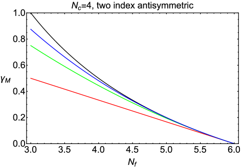
Figure 6: Plot of the exact $\gamma_{M,A_{2}}$ at an IRFP in the non-Abelian Coulomb phase, together with the $O(\Delta_{f}^{p})$ approximations to this result with $1\leq p\leq 3$, for $G={\rm SU}(4)$ and ${\cal R}=A_{2}$, the rank-2 antisymmetric tensor representation. From bottom to top, the curves (with colors online) refer to $\gamma_{M,A_{2},\Delta_{f}}$ (red), $\gamma_{M,A_{2},\Delta_{f}^{2}}$ (green), $\gamma_{M,A_{2},\Delta_{f}^{3}}$ (blue), and the exact $\gamma_{M,A_{2}}$ (black).

In Figs. 6 and 7 we plot the anomalous dimension $\gamma_{M,A_{2}}$ to first, second and third order in $\Delta_{f}$ for $N_{c}=4$ and $N_{c}=5$, together with the respective exact results. Note that for $N_{c}=4$ the $A_{2}$ representation is real, so the meson and baryon operators are equivalent.

For the baryons and antibaryons, we need to distinguish between even and odd values of $N_{c}$. For even $N_{c}=2k$, these are

$$B^{i_{1}\cdots i_{k}}=\frac{1}{2^{k}k!}\epsilon_{a_{1},\ldots,a_{2k}}\Phi^{a_{1}a_{2},i_{1}}\cdots\Phi^{a_{2k-1}a_{2k},i_{k}}$$ (111)

and

$$\tilde{B}_{i_{1}\cdots i_{k}}=\frac{1}{2^{k}k!}\epsilon^{a_{1},\ldots,a_{2k}}\tilde{\Phi}_{a_{1}a_{2},i_{1}}\cdots\tilde{\Phi}_{a_{2k-1}a_{2k},i_{k}}$$ (112)

while for odd $N_{c}$, they are

$$B^{i_{1},\ldots,i_{N_{c}}}=\frac{1}{N_{c}!}\epsilon_{a_{1},\ldots,a_{N_{c}}}\epsilon_{a^{\prime}_{1},\ldots,a^{\prime}_{N_{c}}}\Phi^{a_{1}a^{\prime}_{1},i_{1}}\cdots\Phi^{a_{N_{c}}a^{\prime}_{N_{c}},i_{N_{c}}}$$ (113)

and

$$\tilde{B}_{i_{1},\ldots,i_{N_{c}}}=\frac{1}{N_{c}!}\epsilon^{a_{1},\ldots,a_{N_{c}}}\epsilon^{a^{\prime}_{1},\ldots,a^{\prime}_{N_{c}}}\tilde{\Phi}_{a_{1}a^{\prime}_{1},i_{1}}\cdots\tilde{\Phi}\ _{a_{N_{c}}a^{\prime}_{N_{c}},i_{N_{c}}}$$ (114)

Thus, for even and odd values of $N_{c}$, the respective baryon operators involves $N_{c}/2=k$ and $N_{c}$ $A_{2}$ chiral superfields. Correspondingly, for even and odd $N_{c}$, the contractions of the color indices are analogous to a Pfaffian and a determinant, respectively.

For even $N_{c}$ (denoted $Nce$), the full scaling dimension of the baryon and antibaryon operators is

$$D_{B,A_{2},Nce}=D_{\tilde{B},A_{2},Nce}=\frac{3N_{c}}{4}\Big{[}1-\frac{N_{c}}{N_{f}(N_{c}-2)}\Big{]}\ ,$$ (115)

so the anomalous dimension is

$$\gamma_{B,A_{2},Nce}=\gamma_{\tilde{B},A_{2},Nce}=\frac{N_{c}}{4}\Big{[}\frac{3N_{c}}{N_{f}(N_{c}-2)}-1\Big{]}\ .$$ (116)

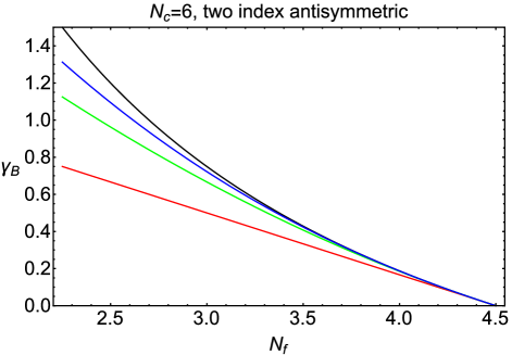
Figure 8: Plot of the exact $\gamma_{B,A_{2}}$ at an IRFP in the non-Abelian Coulomb phase, together with the $O(\Delta_{f}^{p})$ approximations to this result with $1\leq p\leq 3$, for $G={\rm SU}(6)$ and ${\cal R}=A_{2}$. This is the special case of $\gamma_{B,A_{2},Nce}$ in the text for $N_{c}=6$, where the subscript $Nce$ denotes even $N_{c}$. From bottom to top, the curves (with colors online) refer to $\gamma_{B,A_{2},\Delta_{f}}$ (red), $\gamma_{B,A_{2},\Delta_{f}^{2}}$ (green), $\gamma_{B,A_{2},\Delta_{f}^{3}}$ (blue), and the exact $\gamma_{B,A_{2}}$ (black).

We plot $\gamma_{B,A_{2},Nce}$ for $N_{c}=6$ in Fig. 8.

The unitarity constraint from conformal invariance is again $D_{B}>1$, and since $D_{B}=(N_{c}/2)-\gamma_{B}$, this implies the upper bound

$$\gamma_{B,A_{2},Nce}<\frac{N_{c}}{2}-1\ .$$ (117)

If one formally analytically continues $N_{f}$ to the real numbers, as discussed above, so that $N_{f}$ can decrease all the way to $N_{\ell}$ in the NACP, then the maximal value of $\gamma_{B,A_{2}}$ is

$$\gamma_{B,A_{2},Nce}=\frac{N_{c}}{4}\quad{\rm at}\ N_{f}=N_{\ell,A_{2}}\ .$$ (118)

If $N_{c}=4$, then at $N_{\ell}=1$, $\gamma_{B,A_{2},Nce}$ reaches a maximum value of 1, saturating the unitarity upper bound $\gamma_{B,A_{2},Nce}\leq 1$ from conformal invariance. For even $N_{c}\geq 6$, the maximum value of $\gamma_{B,A_{2},Nce}$ as $N_{f}$ formally decreases to $N_{\ell}$ does not saturate the unitarity upper bound, since $N_{c}/4<(N_{c}/2)-1$ for $N_{c}\geq 6$. As $N_{c}\to\infty$ through even values, the ratio of the maximum value of $\gamma_{B,A_{2},Nce}$ evaluated at the formal (non-integral) value of $N_{\ell}$ divided by the unitarity upper bound from conformal invariance approaches 1/2.

For odd $N_{c}$ (denoted $Nco$), the full scaling dimension of the baryon is

$$D_{B,A_{2},Nco}=D_{\tilde{B},A_{2},Nco}=\frac{3N_{c}}{2}\Big{[}1-\frac{N_{c}}{N_{f}(N_{c}-2)}\Big{]}\ ,$$ (119)

so the corresponding anomalous dimension is

$$\gamma_{B,A_{2},Nco}=\gamma_{\tilde{B},A_{2},Nco}=\frac{N_{c}}{2}\Big{[}\frac{3N_{c}}{N_{f}(N_{c}-2)}-1\Big{]}\ .$$ (120)

We plot $\gamma_{B}$ for $N_{c}=5$ in Fig. 9.

The unitarity constraint from conformal invariance is again $D_{B,A_{2}}\geq 1$, and since $D_{B,A_{2},Nco}=(N_{c}/2)-\gamma_{B,A_{2},Nco}$, this implies the upper bound

$$\gamma_{B,A_{2},Nco}<N_{c}-1\ .$$ (121)

With the same analytic continuation as above,

$$\gamma_{N,A_{2},Nco}=\frac{N_{c}}{2}\quad{\rm at}\ N_{f}=N_{\ell,A_{2}}\ .$$ (122)

Even with an analytic continuation of $N_{f}$ from the integers to the real numbers so that $N_{f}$ can actually reach down to $N_{\ell,A_{2}}$, this never saturates the unitarity upper bound from conformal invariance at the lower end of the NACP, since $(N_{c}/2)<N_{c}-1$ for $N_{c}\geq 3$.

VIII Scheme-Independent Calculation and Analysis of $\beta^{\prime}_{IR}$

VIII.1 General

In this section we study the scheme-independent expansion for the derivative of the beta function evaluated at the superconformal IR fixed point, denoted $\beta^{\prime}_{IR}$, in the non-Abelian Coulomb phase. Specifically, we present our calculations of the scheme-independent coefficients $d_{2}$ and $d_{3}$ for general $G$ and ${\cal R}$ and analyze the properties of $d_{4}$ and $\beta^{\prime}_{IR}$ calculated to $O(\Delta_{f}^{4})$ for the case $G={\rm SU}(N_{c})$ and ${\cal R}=F$. For this special case $G={\rm SU}(N_{c})$ and ${\cal R}=F$, quantities equivalent to the $d_{j}$ were calculated in gg for $2\leq j\leq 4$. Our new contributions here are calculations of $d_{2}$ and $d_{3}$ for general $G$ and ${\cal R}$ and also a different analysis of $\beta^{\prime}_{IR}$ in the lower part of the non-Abelian Coulomb phase. One of the reasons for interest in this derivative is that $\beta^{\prime}_{IR}$ is equivalent grisaru97 to the anomalous dimension of the Konishi supercurrent konishi .

VIII.2 Calculation via Series Expansion in $\alpha$

It is useful first to review the calculation of $\beta^{\prime}_{IR}$ in bc ; lnn using a conventional series expansion in powers of $\alpha$ up to three-loop order. In general, from Eq. (4), it follows that

$$\beta^{\prime}=-2\sum_{\ell=1}^{\infty}(\ell+1)b_{\ell}\,a^{\ell}\ .$$ (123)

where $a=\alpha/(4\pi)=g^{2}/(16\pi^{2})$. Evaluating the $n$-loop truncation of this series at the IR zero in the $n$-loop beta function, $\alpha_{IR,n\ell}$ yields the $n$-loop value of the derivative, $\beta^{\prime}_{IR,n\ell}$. Since $b_{1}$ and $b_{2}$ are scheme-independent, this is also true of $\beta^{\prime}_{IR,2\ell}$, for which one finds bc

$$\beta^{\prime}_{IR,2\ell} = -\frac{2b_{1}^{2}}{b_{2}}$$ (124)

$$= \frac{(3C_{A}-2T_{f}N_{f})^{2}}{2(C_{A}+2C_{f})T_{f}N_{f}-3C_{A}^{2}}\ .$$ (126)

For general $G$ and ${\cal R}$, $\beta^{\prime}_{IR,2\ell}$ increases monotonically as $N_{f}$ decreases from $N_{u}$ in the NACP. At the three-loop level, the condition for the IR zero is the quadratic equation $b_{1}+b_{2}a+b_{3}a^{2}=0$, whence, $a^{2}=-(b_{1}+b_{2}a)/b_{3}$. Substituting this into Eq. (123), one has

$$\beta^{\prime}_{IR,3\ell}=2a_{IR,3\ell}(2b_{1}+b_{2}a_{IR,3\ell})\ ,$$ (127)

where $a_{IR,3\ell}$ is the physical root of the quadratic equation above. The three-loop calculation in bc used the value of $b_{3}$ in the $\overline{\rm DR}$ scheme. As mentioned above, we have found that the four-loop beta function does not exhibit a physical IR zero over a substantial interval of $N_{f}$ in the NACP. That is, extracting the prefactor of $a^{2}$ in $\beta_{4\ell}$, we have found that the cubic equation $b_{1}+b_{2}a+b_{3}a^{2}+b_{4}a^{3}=0$ has no real positive zero in this range of $N_{f}$. We will discuss this further in the subsection on the LNN limit.

In the special case $G={\rm SU}(N_{c})$ and ${\cal R}=F$, Eq. (126) reduces to

$$\beta^{\prime}_{IR,2\ell}=\frac{N_{c}(3N_{c}-N_{f})^{2}}{(2N_{c}^{2}-1)N_{f}-3N_{c}^{2}}\ .$$ (128)

To write an expression for the three-loop derivative, $\beta^{\prime}_{IR,3\ell}$, it is convenient first to define two auxiliary polynomials in $N_{c}$ and $N_{f}$:

$$D_{s} = -21N_{c}^{5}+21N_{c}^{4}N_{f}-4N_{c}^{3}N_{f}^{2}-9N_{c}^{2}N_{f}$$ (129)

$$+ 3N_{c}N_{f}^{2}-2N_{f}$$ (131)

and

$$C_{s} = -54N_{c}^{6}+72N_{c}^{5}N_{f}-29N_{c}^{4}N_{f}^{2}+N_{c}^{3}N_{f}(4N_{f}^{2}-21)$$ (132)

$$+ 14N_{c}^{2}N_{f}^{2}-3N_{c}N_{f}(N_{f}^{2}+2)+3N_{f}^{2}\ .$$ (134)

Then

$$\beta^{\prime}_{IR,3\ell}=\frac{N_{c}}{D_{s}}\Big{[}3N_{c}^{3}-2N_{c}^{2}N_{f}+N_{f}+\sqrt{C_{s}}\ \Big{]}\ .$$ (135)

We will discuss these $n$-loop calculations further in the LNN limit (178) below.

VIII.3 Calculation via Series Expansion in $\Delta_{f}$

Proceeding the scheme-independent $\Delta_{f}$ expansion, we calculate, for general $G$ and ${\cal R}$,

$$d_{2}=\frac{2T_{f}^{2}}{3C_{A}C_{f}}$$ (136)

and

$$d_{3}=\frac{2T_{f}^{3}(C_{A}+2C_{f})}{(3C_{A}C_{f})^{2}}\ .$$ (137)

To our knowledge, these results are new. If $G={\rm SU}(N_{c})$ and ${\cal R}=F$, then these take the form

$${\rm SU}(N_{c}),\ R=F:\quad d_{2,F}=\frac{1}{3(N_{c}^{2}-1)}$$ (138)

and

$$d_{3,F}=\frac{2N_{c}^{2}-1}{9N_{c}(N_{c}^{2}-1)^{2}}\ .$$ (139)

For this case of $G={\rm SU}(N_{c})$ and ${\cal R}=F$, the next-higher-order coefficient is

$$d_{4,F}=\frac{(N_{c}^{4}-2N_{c}^{2}+5)-18N_{c}^{2}(N_{c}^{2}+1)\zeta_{3}}{108N_{c}^{2}(N_{c}^{2}-1)^{3}}\ ,$$ (140)

where $\zeta_{s}=\sum_{n=1}^{\infty}n^{-s}$ is the Riemann zeta function. These results for $d_{j}$, $2\leq j\leq 4$ for $G={\rm SU}(N_{c})$ and ${\cal R}=F$ agree with equivalent quantities given in gg . From these results for $d_{j}$, $2\leq j\leq 4$, it is evident that the coefficients $d_{j}$ in expansion (39) for $\beta^{\prime}_{IR}$ does not have the form of a geometric series. This is in contrast to our theorem above and the resultant Eq. (53) for the coefficient $f_{\Phi_{\rm prod},j}$ in expansion of the anomalous dimension of a composite chiral superfield $\Phi_{\rm prod}$ in powers of $\Delta_{f}$, which showed that the latter series is a geometric series. This is completely consistent with our theorem, since the Konishi supercurrent is not a (composite) chiral superfield.

The coefficients $d_{2}$ and $d_{3}$ are manifestly positive for any $G$ and $R$. We find that $d_{4}$ is negative for all physical $N_{c}\geq 2$. These are qualitatively the same results that we found in dex for non-supersymmetric theories, namely that for arbitrary $G$ and $R$, $d_{2}$ and $d_{3}$ are positive and in the case $G={\rm SU}(N_{c})$ and ${\cal R}=F$, $d_{4}$ is negative for all $N_{c}\geq 2$.

The perfect agreement that we have found between the $\kappa_{j}$ that we have calculated and the exact result (60) suggests that the same agreement could hold for the $d_{j}$ with $1\leq j\leq 3$ that we have calculated. That is, these should also agree with the $d_{j}$ coefficients obtained from the expansion of the exact $\beta^{\prime}_{IR}$ as a series in powers of $\Delta_{f}$ as expressed in Eq. (39). The only difference is that in contrast to $\gamma_{M}$, one does not have an exact closed-form expression for $\beta^{\prime}_{IR}$ with which to compare in this ${\cal N}=1$ supersymmetric gauge theory.

In Table 4 we list the (scheme-independent) values that we calculate for $\beta^{\prime}_{IR,F,\Delta_{f}^{p}}$ with $2\leq p\leq 4$ for the illustrative gauge groups $G={\rm SU}(2)$, SU(3), and SU(4), as functions of $N_{f}$ in the respective non-Abelian Coulomb phase intervals given in Eq. (12). Numerically,

$${\rm SU}(2):\quad\beta^{\prime}_{IR,F,\Delta_{f}^{4}} = \Delta_{f}^{2}\Big{[}0.11111+(4.3210\times 10^{-2})\Delta_{f}-(3.5986\times 10^{-2})\Delta_{f}^{2}\ \Big{]}$$ (141)

$${\rm SU}(3):\quad\beta^{\prime}_{IR,F,\Delta_{f}^{4}} = \Delta_{f}^{2}\Big{[}4.1667\times 10^{-2}+(0.98380\times 10^{-2})\Delta_{f}-(3.7763\times 10^{-3})\Delta_{f}^{2}\ \Big{]}$$ (144)

and

$${\rm SU}(4):\quad\beta^{\prime}_{IR,F,\Delta_{f}^{4}} = \Delta_{f}^{2}\Big{[}2.2222\times 10^{-2}+(3.8272\times 10^{-3})\Delta_{f}-(0.96987\times 10^{-3})\Delta_{f}^{2}\ \Big{]}\ .$$ (147)

where the numerical coefficients are listed to the given floating-point accuracy.

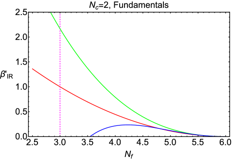
Figure 10: Plot of $\beta^{\prime}_{IR,\Delta_{f}^{p}}$ with $2\leq p\leq 4$ for $G={\rm SU}(2)$ and ${\cal R}=F$, as a function of $N_{f}$ at an IRFP in the non-Abelian Coulomb phase for this theory. At $N_{f}=4$, from bottom to top, the curves (with colors online) refer to $\beta^{\prime}_{IR,\Delta_{f}^{4}}$ (blue), $\beta^{\prime}_{IR,\Delta_{f}^{2}}$ (red), and $\beta^{\prime}_{IR,\Delta_{f}^{3}}$ (green).

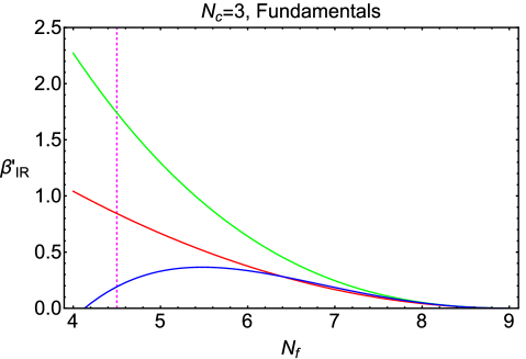
Figure 11: Plot of $\beta^{\prime}_{IR,\Delta_{f}^{p}}$ with $2\leq p\leq 4$ for $G={\rm SU}(3)$ and ${\cal R}=F$, as a function of $N_{f}$ at an IRFP in the non-Abelian Coulomb phase for this theory. At $N_{f}=5$, from bottom to top, the curves (with colors online) refer to $\beta^{\prime}_{IR,\Delta_{f}^{4}}$ (blue), $\beta^{\prime}_{IR,\Delta_{f}^{2}}$ (red), and $\beta^{\prime}_{IR,\Delta_{f}^{3}}$ (green).

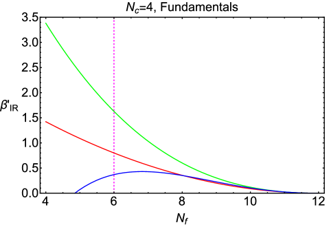
Figure 12: Plot of $\beta^{\prime}_{IR,\Delta_{f}^{p}}$ with $2\leq p\leq 4$ for $G={\rm SU}(4)$ and ${\cal R}=F$, as a function of $N_{f}$ at an IRFP in the non-Abelian Coulomb phase for this theory. At $N_{f}=6$, from bottom to top, the curves (with colors online) refer to $\beta^{\prime}_{IR,\Delta_{f}^{4}}$ (blue), $\beta^{\prime}_{IR,\Delta_{f}^{2}}$ (red), and $\beta^{\prime}_{IR,\Delta_{f}^{3}}$ (green).

In Figs. 10-12 we show plots of $\beta^{\prime}_{IR,F,\Delta_{f}^{p}}$ with $2\leq p\leq 4$ for these three theories for $N_{f}$ in the respective non-Abelian Coulomb phase interval, $(3/2)N_{c}<N_{f}<3N_{c}$. (The plots also show the behavior for $N_{f}$ values slightly below the lower end of the NACP.)

We next address the question of how well, for a given $G$, ${\cal R}$, and $N_{f}$, the $\Delta_{f}$ expansion for $\beta^{\prime}_{IR}$ converges in this ${\cal N}=1$ supersymmetric gauge theory. We had carried out a similar analysis for the $\Delta_{f}$ expansions for $\gamma_{M}$ and $\beta^{\prime}_{IR}$ in our previous work gtr -dexl . The $\Delta_{f}$ expansion is a series expansion about $\Delta_{f}=0$, i.e., $N_{f}=N_{u}$, at the upper end of the non-Abelian Coulomb phase. As $\Delta_{f}$ increases, i.e., as $N_{f}$ decreases below $N_{u}$, one needs progressively more terms in this expansion to obtain an accurate estimate of a given quantity. In general, if $f(z)$ is an analytic function at $z=0$, then it has a Taylor series expansion

$$f(z)=\sum_{j=1}^{\infty}f_{j}z^{j}\ .$$ (150)

The radius of convergence of this series, $z_{c}$, can be determined by the ratio test as

$$z_{c}=\lim_{j\to\infty}\frac{|f_{j-1}|}{|f_{j}|}\ .$$ (151)

With the $\Delta_{f}$ expansion for $\beta^{\prime}_{IR}$ considered as a Taylor series expansion, one could, in principle, calculate the radius of convergence ($cv$), $|\Delta_{f{,\rm cnv}}|$ as

$$\Delta_{f,{\rm cnv}}=\lim_{j\to\infty}\frac{|d_{j}|}{|d_{j+1}|}\ .$$ (152)

Clearly, it is not possible to apply this test precisely here for $\beta^{\prime}_{IR}$ as a series in powers of $\Delta_{f}$, since one does not know the $d_{j}$ for $j\to\infty$. Nevertheless, one can obtain a rough estimate of the radius of convergence by calculating the ratios of adjacent coefficients for the first few $d_{j}$. We define the estimate of the radius of convergence given by the ratio $|d_{j}/d_{j+1}|$ as

$$\Delta_{f,{\rm cnv},(j,j+1)}=\frac{|d_{j}|}{|d_{j+1}|}\ .$$ (153)

Correspondingly, for a given $G$ and $R$, the minimum value of $N_{f}$ to which the small-$\Delta_{f}$ expansion would be estimated to be convergent (denoted $mc$ for “minimum ($N_{f}$) for convergence”) is

$$N_{f,{\rm mc},(j,j+1)}=N_{u}-\Delta_{f,{\rm cnv},(j,j+1)}\ ,$$ (154)

where $N_{u}$ was given in Eq. (8). For general $G$ and ${\cal R}$, we have

$$\Delta_{f,{\rm cnv},(j,j+1)}=\frac{d_{2}}{d_{3}}=\frac{3C_{A}C_{f}}{T_{f}(C_{A}+2C_{f})}\ ,$$ (155)

and hence

$$N_{f,{\rm mc},(2,3)}=\frac{3C_{A}^{2}}{2T_{f}(C_{A}+2C_{f})}\ .$$ (156)

This may lie above or below the lower end of the non-Abelian Coulomb phase at $N_{\ell}$, as determined by the difference

$$N_{f,mc,(2,3)}-N_{\ell}=\frac{3C_{A}(C_{A}-2C_{f})}{4T_{f}(C_{A}+2C_{f})}\ .$$ (157)

For example, for $G={\rm SU}(N_{c})$, this difference is positive for the fundamental representation, but negative for the adjoint representation.

We now focus on the case of main interest here, namely $G={\rm SU}(N_{c})$ and ${\cal R}=F$. For this case,

$$\frac{d_{2,F}}{d_{3,F}}=\frac{3N_{c}(N_{c}^{2}-1)}{2N_{c}^{2}-1}\ ,$$ (158)

so that

$$N_{f,{\rm mc},(2,3)}=\frac{3N_{c}^{3}}{2N_{c}^{2}-1}\ .$$ (159)

Parenthetically, we observe that this difference is equal to the special case of $N_{f,b2z}$ (given in general in Eq. (17)) for $G={\rm SU}(N_{c})$ and ${\cal R}=F$. The value $N_{f,mc,(2,3)}$ lies above the lower end of the non-Abelian Coulomb phase, as is evident from the difference

$$N_{f,{\rm mc},(2,3)}-N_{\ell}=\frac{3N_{c}^{2}}{2(2N_{c}^{2}-1)}\ .$$ (160)

As $N_{c}\to\infty$, this difference approaches zero.

For the ratio of the next higher-order coefficients, we find

$$\frac{d_{3,F}}{|d_{4,F}|}=\frac{12N_{c}(N_{c}^{2}-1)(2N_{c}^{2}-1)}{18N_{c}^{2}(N_{c}^{2}+1)\zeta_{3}-(N_{c}^{4}-2N_{c}^{2}+5)}\ ,$$ (161)

so

$$N_{f,{\rm mc},(3,4)}=\frac{3N_{c}[18N_{c}^{2}(N_{c}^{2}+1)\zeta_{3}-9N_{c}^{4}+14N_{c}^{2}-9]}{18N_{c}^{2}(N_{c}^{2}+1)\zeta_{3}-(N_{c}^{4}-2N_{c}^{2}+5)}\ .$$ (162)

This value lies above the lower end of the NACP, as is evident from the difference

$$N_{f,{\rm mc},(3,4)}-N_{\ell}=$$ (163)

(164)

$$\frac{3N_{c}[18N_{c}^{2}(N_{c}^{2}+1)\zeta_{3}-17N_{c}^{4}+26N_{c}^{2}-13]}{18N_{c}^{2}(N_{c}^{2}+1)\zeta_{3}-(N_{c}^{4}-2N_{c}^{2}+5)}\ .$$ (165)

(166)

(167)

In Table 5 we list values of $N_{\ell}$, $N_{u}$, $N_{f,{\rm mc},(2,3)}$, $N_{f,{\rm mc},(2,3)}-N_{\ell}$, $N_{f,{\rm mc},(3,4)}$, and $N_{f,{\rm mc},(3,4)}-N_{\ell}$ for the illustrative cases $N_{c}=2,\ 3,\ 4$. Thus, our analysis of the first two ratios of coefficients in the small-$\Delta_{f}$ series expansion for $\beta^{\prime}_{IR}$ suggests that the small-$\Delta_{f}$ expansion for $\beta^{\prime}_{IR}$ may be reliable over a substantial portion of the non-Abelian Coulomb phase, including, in particular, the upper and middle parts. In general, one would not expect the small-$\Delta_{f}$ expansion to apply reliably for small values $N_{f}$, where the properties of the theory are qualitatively different from the properties in the non-Abelian Coulomb phase.

These results on the convergence of the small-$\Delta_{f}$ expansion (39) for $\beta^{\prime}_{IR}$ may be compared with our results for the convergence of the corresponding expansion (41) for $\gamma_{M}$. As recalled above, we found from our calculation of the coefficients $\kappa_{j}$ in the latter expansion that they agreed perfectly with the Taylor series expansion of the exact result (60). This Taylor series expansion of (60) converges throughout the entire non-Abelian Coulomb phase. Superficially, from the analysis of the coefficients $d_{j}$ with $j=2,\ 3,\ 4$ in the small-$\Delta_{f}$ series expansion of $\beta^{\prime}_{IR}$, one might infer that this series expansion might not converge as rapidly as the small-$\Delta_{f}$ expansion for $\gamma_{M}$ gg . However, one would need more terms to get a better estimate of the actual region of convergence of the series expansion of $\beta^{\prime}_{IR}$ in powers of $\Delta_{f}$. Especially in view of our proof above that the series expansion in powers of $\Delta_{f}$ of the anomalous dimension $\gamma_{\Phi_{\rm prod}}$ converges throughout the entirety of the non-Abelian Coulomb phase, we believe that it is plausible that the same is true of the corresponding series for $\beta^{\prime}_{IR}$.

For general $G$ and ${\cal R}$, since $d_{2}$ and $d_{3}$ are positive, $\beta^{\prime}_{IR}$ increases (initially quadratically) from 0 as $\Delta_{f}$ increases from 0, i.e., as $N_{f}$ decreases below its upper bound from asymptotic freedom, $N_{u}$. In the class of theories with $G={\rm SU}(N_{c})$ and ${\cal R}=F$, we have calculated the next higher-order coefficient, $d_{4,F}$ and have shown that it is negative for all physical $N_{c}$. It is of interest to investigate the consequences of the fact that $d_{4,F}$ is negative, bearing in mind the cautionary remarks concerning the range in $N_{f}$ in which the small-$\Delta_{f}$ may be reasonably reliable. Because $d_{4,F}$ is negative, as $\Delta$ increases from 0, i.e., as $N_{f}$ decreases from $N_{u}$, the $d_{4}\Delta_{f}^{4}$ term in $\beta^{\prime}_{IR}$ eventually stops the initial increase in $\beta^{\prime}_{IR,\Delta_{f}^{4}}$ and, for smaller $N_{f}$, causes $\beta^{\prime}_{IR,\Delta_{f}^{4}}$ to decrease. If one were to use the $\Delta_{f}$ expansion for sufficiently small values of $N_{f}$, then the series for $\beta^{\prime}_{IR}$ calculated to $O(\Delta_{f}^{4})$, i.e., $\beta^{\prime}_{IR,\Delta_{f}^{4}}$, would pass through zero to negative values. We first determine the value of $\Delta_{f}$, or equivalently, $N_{f}$, at which $\beta^{\prime}_{IR,\Delta_{f}^{4}}$ vanishes. The condition that $\beta^{\prime}_{IR,\Delta_{f}^{4}}=0$ is the equation

$$\Delta_{f}^{2}(d_{2}+d_{3}\,\Delta_{f}+d_{4}\,\Delta_{f}^{2})=0\ .$$ (168)

Aside from the solution $\Delta_{f}=0$, i.e., $N_{f}=N_{u}$, this equation has two solutions, corresponding to the roots of the quadratic factor. Of these, we denote the relevant one as $\Delta_{0}=N_{u}-N_{f,0}$. We calculate

$$N_{f,0}=\frac{3N_{c}\Big{[}N_{c}^{4}(-5+18\zeta_{3})+2N_{c}^{2}(4+9\zeta_{3})-7-2(N_{c}^{2}-1)\sqrt{S_{0}}}{N_{c}^{4}(18\zeta_{3}-1)+2N_{c}^{2}(1+9\zeta_{3})-5}\ ,$$ (169)

where

$$S_{0}=3N_{c}^{4}(1+6\zeta_{3})+2N_{c}^{2}(-1+9\zeta_{3})-4\ .$$ (170)

(The other root of the quadratic factor, with the opposite sign in front of the square root, is greater than $N_{u}$ and hence is not relevant here, since we restrict $N_{f}<N_{u}$ for asymptotic freedom.) Numerically, for the illustrative values $N_{c}=2,\ 3,\ 4$, our expression for $N_{f,0}$ (understood to be continued from the positive integers to the positive real numbers) takes the respective values 3.5427, 4.1294, and 4.8496. In these three cases, as is evident from Table 5, $N_{\ell}$ has the respective values =3,  4.5,  6, so that for ${\cal R}=F$ and $G={\rm SU}(2)$, $N_{f,0}>N_{\ell}$, while for SU(3) and SU(4), $N_{f,0}<N_{\ell}$.

Using electric-magnetic duality, it has been concluded that for $G={\rm SU}(N_{c})$ and ${\cal R}=F$, $\beta^{\prime}_{IR}$ vanishes quadratically at the lower end of the non-Abelian Coulomb phase at $N_{f}=N_{\ell}=(3/2)N_{c}$ grisaru97 :

$$\beta^{\prime}_{IR}=\frac{28}{3}\,\Big{(}\frac{N_{f}}{N_{c}}-\frac{3}{2}\Big{)}^{2}\quad{\rm as}\ N_{f}\searrow\frac{3N_{c}}{2}\ .$$ (171)

Given the fact that our $\Delta_{f}$ expansion starts from the other (i.e., the upper) end of the non-Abelian Coulomb phase, we would not expect our calculations of $\beta^{\prime}_{IR}$ to $O(\Delta_{f}^{4})$ for this theory to precisely reproduce this behavior at $N_{f}=(3/2)N_{c}$. Taking this into account, our numerical results on $N_{f,0}$ are consistent with the behavior in (171). It should be noted that the three values listed above for $N_{f,0}$ actually lie below the minimum values where where our estimates indicate that the small-$\Delta_{f}$ series is reliable, namely the values 4.8, 6.4, and 8.05 for $N_{c}=2,\ 3,\ 4$, respectively, as listed in Table 5. A general statement is that our calculations of series expansions for $\beta^{\prime}_{IR}$ in both the nonsupersymmetric gauge theory dex ; dexs ; dexl and the results present here for the supersymmetric gauge theory show qualitatively quite different behavior than we have found for both $\gamma_{M}$ and $\gamma_{B}$. In the latter two cases, all of the coefficients in the small-$\Delta_{f}$ expansion are positive, leading to the two monotonicity theorems mentioned above.

IX Results in the Limit of Large $N_{c}$ and $N_{f}$ with $N_{f}/N_{c}$ Fixed

IX.1 General

For this class of theories with $G={\rm SU}(N_{c})$ and ${\cal R}=F$, an interesting limit is

$$LNN:\quad N_{c}\to\infty\ ,\quad N_{f}\to\infty$$ (172)

(173)

$${\rm with}\ r\equiv\frac{N_{f}}{N_{c}}\ {\rm fixed\ and\ finite}$$ (174)

(175)

$${\rm and}\ \ \xi(\mu)\equiv\alpha(\mu)N_{c}\ {\rm is\ a\ finite\ function\ of}\ \mu\ .$$ (176)

(177)

(178)

We will use the symbol $\lim_{LNN}$ for this limit, where “LNN” stands for “large $N_{c}$ and $N_{f}$” with the constraints in Eq. (178) imposed. This is sometimes called the ’t Hooft-Veneziano limit.

We define the following quantities in this limit:

$$\xi=4\pi x=\lim_{LNN}\alpha N_{c}\ ,$$ (179)

$$r_{u}=\lim_{LNN}\frac{N_{u}}{N_{c}}\ ,$$ (180)

and

$$r_{\ell}=\lim_{LNN}\frac{N_{\ell}}{N_{c}}\ ,$$ (181)

with values

$$r_{u}=3\ ,\quad\quad r_{\ell}=\frac{3}{2}\ .$$ (182)

These quantities are listed in Table 6. Thus, the non-Abelian Coulomb phase occurs for $r$ in the interval

$${\rm LNN,\ \ NACP}:\quad\frac{3}{2}<r<3\ .$$ (183)

We define the scaled scheme-independent expansion parameter for the LNN limit

$$\Delta_{r}\equiv\frac{\Delta_{f}}{N_{c}}=r_{u}-r=3-r\ .$$ (184)

As $r$ decreases from $r_{u}$ to $r_{\ell}$ in the non-Abelian Coulomb phase, $\Delta_{r}$ increases from 0 to a maximal value

$$(\Delta_{r})_{\rm max}=r_{u}-r_{\ell}=\frac{3}{2}\quad{\rm for}\ r\in{\rm NACP}\ .$$ (185)

(186)

(187)

IX.2 $\gamma_{M}$ in the LNN Limit

For the analysis of $\gamma_{M}$ at the superconformal IRFP, we define rescaled coefficients $\hat{\kappa}_{j,F}$

$$\hat{\kappa}_{j,F}\equiv\lim_{N_{c}\to\infty}N_{c}^{j}\,\kappa_{j,F}$$ (188)

that are finite in this LNN limit. The anomalous dimension $\gamma_{IR}$ is also finite in this limit and is given by

$${\cal R}=F:\quad\lim_{LNN}\gamma_{M,LNN}=\sum_{j=1}^{\infty}\hat{\kappa}_{j,F}\Delta_{r}^{j}\ .$$ (189)

In this LNN limit, the exact result for $\gamma_{M,LNN}$ (60) takes the form

$$\gamma_{M,LNN}=\frac{\frac{\Delta_{r}}{3}}{1-\frac{\Delta_{r}}{3}}\ ,$$ (190)

so that

$$\hat{\kappa}_{j,F}=\frac{1}{3}\quad\forall\ j\ .$$ (191)

IX.3 Rescaled $\gamma_{B}$ in the LNN Limit

To construct a rescaled anomalous dimension at the superconformal IRFP that is finite in the LNN limit, we define

$$\hat{\gamma}_{B}\equiv\lim_{LNN}\frac{\gamma_{B}}{N_{c}}\ ,$$ (192)

and similarly with $\hat{\gamma}_{\tilde{B}}=\hat{\gamma}_{B}$. By construction, these rescaled baryon anomalous dimensions are finite in the LNN limit and have the common value

$$\lim_{LNN}\hat{\gamma}_{B}=\frac{1}{2}\Big{(}\frac{3}{r}-1\Big{)}\ .$$ (193)

IX.4 $\beta^{\prime}_{IR}$ in the LNN Limit

The rescaled beta function that is finite and nontrivial in the LNN limit is

$$\beta_{\xi}\equiv\frac{d\xi}{dt}=\lim_{LNN}\beta_{\alpha}N_{c}\ ,$$ (194)

with the series expansion

$$\beta_{\xi}\equiv\frac{d\xi}{dt}=-8\pi x\sum_{\ell=1}^{\infty}\hat{b}_{\ell}x^{\ell}=-2\xi\sum_{\ell=1}^{\infty}\tilde{b}_{\ell}\xi^{\ell}\ ,$$ (195)

where

$$\hat{b}_{\ell}=\lim_{LNN}\frac{b_{\ell}}{N_{c}^{\ell}}\ ,\quad\tilde{b}_{\ell}=\lim_{LNN}\frac{\bar{b}_{\ell}}{N_{c}^{\ell}}\ .$$ (196)

The first two rescaled coefficients of the beta function, which are scheme-independent, are

$$\hat{b}_{1}=3-r$$ (197)

and

$$\hat{b}_{2}=2(3-2r)\ .$$ (198)

In the $\overline{\rm DR}$ scheme,

$$\hat{b}_{3}=21-21r+4r^{2}$$ (199)

and

$$\hat{b}_{4}=2[51-66r+3(7+2\zeta_{3})r^{2}]\ .$$ (200)

In the LNN limit, one has the scheme-independent two-loop result

$$x_{IR,2\ell}=-\frac{\hat{b}_{1}}{\hat{b}_{2}}=\frac{3-r}{2(2r-3)}\ .$$ (201)

At the three-loop level, $x_{IR,3\ell}$ is the physical root among the two roots of the quadratic equation $\hat{b}_{1}+\hat{b}_{2}x+\hat{b}_{3}x^{2}=0$. It is convenient to define two auxiliary polynomials:

$$C_{r}=\lim_{LNN}\frac{C_{s}}{N_{c}^{6}}=-54+72r-29r^{2}+4r^{3}$$ (202)

and

$$D_{r}=\lim_{LNN}\frac{D_{s}}{N_{c}^{5}}=-21+21r-4r^{2}\ .$$ (203)

Then

$$x_{IR,3\ell}=\frac{2[-(2r-3)+\sqrt{C_{s}}\ ]}{D_{s}}\ .$$ (204)

These inputs were used to calculate $\beta^{\prime}_{IR}$ in the LNN limit bc ; lnn . At two-loop order, one has the scheme-independent result,

$$\beta^{\prime}_{\xi,IR,2\ell}=\frac{(3-r)^{2}}{2r-3}\ .$$ (205)

At the three-loop order bc ; lnn

$$\beta^{\prime}_{\xi,IR,3\ell}=2x_{IR,3\ell}(2b_{1}+b_{2}x_{IR,3\ell})$$ (206)

$$= 2(3-r)\Big{[}-(2r-3)+\sqrt{C_{r}}\ \Big{]}\times$$ (208)

$$\times \bigg{[}1+\frac{2\Big{[}-(2r-3)+\sqrt{C_{r}}\ \Big{]}}{D_{s}}\ \bigg{]}\ .$$ (210)

We list the values of $\beta^{\prime}_{IR,2\ell}$ and $\beta^{\prime}_{IR,3\ell}$ in Table 7.

We find that the four-loop beta function does not exhibit a physical (i.e., real, positive) IR zero over a substantial portion of the NACP interval $3/2<r<3$. Specifically, extracting the prefactor proportional to $x^{2}$ in $\beta_{\xi,4\ell}$, we find that, as $r$ decreases from its upper bound of $r=3$ in the NACP, the equation $\hat{b}_{1}+\hat{b}_{2}x+\hat{b}_{3}x^{2}+\hat{b}_{4}=0$ ceases to exhibit a physical zero as $r$ decreases below $r_{0}=2.6165$. We recall that we found that although the $n$-loop beta function had a physical IR zero for $n=2$, 3, and 4 loops in the corresponding nonsupersymmetric SU($N_{c}$) theory with $N_{f}$ fermions with ${\cal R}=F$, this was not the case at the five-loop level flir , and in the LNN limit, as $r$ decreased below its upper limit of 5.5, the five-loop beta beta function ceased to exhibit a physical IR zero as $r$ decreased through the value $r_{cx}=4.3226$ (as given in Eq. (5.3) of dexl ). Thus, this complication appears at one loop lower (i.e. at the four-loop level) in the present supersymmetric theory, as compared with the case of the nonsupersymmetric theory with the same $G$ and $R$. This shows again the advantage of the scheme-independent expansion method, since it does circumvents the explicit extraction of $\alpha_{IR,n\ell}$ (here, $x_{n,\ell}$ in the LNN limit) in order to calculate values of physical quantities at the IRFP.

For the scheme-independent expansion, in addition to the rescaled quantity $\Delta_{r}$ defined in Eq. (184), we define the rescaled coefficient

$$\hat{d}_{j,F}=\lim_{LNN}N_{c}^{j}\,d_{j,F}\ ,$$ (211)

which is finite. Then each term

$$\lim_{LNN}d_{j,F}\Delta_{r}^{j} = \lim_{LNN}(N_{c}^{j}d_{j,F})\Big{(}\frac{\Delta_{r}}{N_{c}}\Big{)}^{j}$$ (212)

$$= \hat{d}_{j,F}\Delta_{r}^{j}\ .$$ (214)

is finite in this limit. Thus, writing $\lim_{LNN}\beta^{\prime}_{IR}$ as $\beta^{\prime}_{IR,LNN}$ for this ${\cal R}=F$ case, we have

$$\beta^{\prime}_{IR,LNN}=\sum_{j=1}^{\infty}\hat{d}_{j,F}\Delta_{r}^{j}\ .$$ (215)

From our results (138), (139), and (140), it follows that

$$\hat{d}_{2,F}=\frac{1}{3}\ ,$$ (216)

$$\hat{d}_{3,F}=\frac{2}{9}=0.22222\ ,$$ (217)

and

$$\hat{d}_{4,F}=-\frac{(18\zeta_{3}-1)}{108}=-0.19108\ .$$ (218)

Thus, in this LNN limit, to $O(\Delta_{r}^{4})$,

$$\beta^{\prime}_{IR,LNN,\Delta_{r}^{4}}=\Delta_{r}^{2}\Big{[}\frac{1}{3}+\frac{2}{9}\,\Delta_{r}-\Big{(}\frac{18\zeta_{3}-1}{108}\Big{)}\,\Delta_{r}^{2}\Big{]}\ .$$ (219)

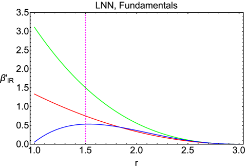
Figure 13: Plot of $\beta^{\prime}_{IR,LNN,\Delta_{r}^{p}}$ with $2\leq p\leq 4$ as a function of $r$ in the LNN limit (178), for $r$ at an IRFP in the non-Abelian Coulomb phase. At $r=1.6$, from bottom to top, the curves (with colors online) refer to $\beta^{\prime}_{IR,LNN,\Delta_{r}^{4}}$ (blue), $\beta^{\prime}_{IR,LNN,\Delta_{r}^{2}}$ (red), and $\beta^{\prime}_{IR,LNN,\Delta_{r}^{3}}$ (green).

In Table 7 we list the (scheme-independent) values that we calculate for $\beta^{\prime}_{IR,LNN,\Delta_{r}^{p}}$ and in Fig. 13, we plot $\beta^{\prime}_{IR,LNN,\Delta_{r}^{p}}$ with $2\leq p\leq 4$, as functions of $r$ in the non-Abelian Coulomb phase interval $3/2<r<3$. (The plot also shows the behavior slightly below the lower end of the NACP.)

To obtain a rough estimate of the interval in $r$ in which this small-$\Delta_{r}$ expansion is reliable, we follow the same procedure as before for finite $N_{c}$ and $N_{f}$. Analogously to Eqs. (153) and (154), we define

$$(\Delta_{r})_{{\rm cnv},(j,j+1)}=\frac{|\hat{d}_{j}|}{|\hat{d}_{j+1}|}$$ (220)

and

$$r_{{\rm mc},(j,j+1)}=r_{u}-\Delta_{r,{\rm cnv},(j,j+1)}\ .$$ (221)

We calculate

$$(\Delta_{r})_{{\rm cnv},(2,3)}=\frac{3}{2}$$ (222)

and

$$(\Delta_{r})_{cnv,(3,4)}=\frac{24}{18\zeta_{3}-1}=1.16296\ ,$$ (223)

so that

$$r_{{\rm mc},(2,3)}=\frac{3}{2}$$ (224)

and

$$r_{{\rm mc},(3,4)}=\frac{27(2\zeta_{3}-1)}{18\zeta_{3}-1}=1.8370$$ (225)

Since the lower end of the non-Abelian Coulomb phase occurs at $r_{\ell}=3/2$, this analysis suggests that the small-$\Delta_{r}$ expansion may be reasonably reliable for a substantial part of this phase, extending down from $r=3$ to around $r\sim 1.8$.

In the present LNN limit, the condition that $\beta^{\prime}_{IR,LNN}=0$ is satisfied at $\Delta_{r}=0$, i.e., $r=3$, and at the relevant solution of the quadratic factor in Eq. (219). We define

$$\Delta_{r,0}=3-r_{0}\ ,$$ (226)

with

$$r_{0}=\lim_{LNN}\frac{N_{f,0}}{N_{c}}\ .$$ (227)

We calculate

$$r_{0}=\frac{3\Big{[}18\zeta_{3}-5-2\sqrt{3(1+6\zeta_{3})}\ \Big{]}}{18\zeta_{3}-1}=0.975415\ ,$$ (228)

where the numerical value is given to the indicated floating-point accuracy. (The other root of the quadratic, with the opposite sign in front of the square root, is $r=3.861627$, which is greater than $r_{u}=3$ and hence is not relevant.) Evidently, $r_{0}$ is less $r_{\ell}=1.5$, i.e., it lies below the lower end of the non-Abelian Coulomb phase and well below the region in $r$ where the small-$\Delta_{r}$ expansion is expected to be reliable, based on our analysis of ratios of $\hat{d}_{j}$ above.

In the LNN limit, the result (171) from grisaru97 is

$$\beta^{\prime}_{IR}=\frac{28}{3}\Big{(}r-\frac{3}{2}\Big{)}^{2}\quad{\rm as}\ r\searrow\frac{3}{2}\ .$$ (229)

Analogously to our discussion above for finite $N_{c}$ and $N_{f}$, here in the LNN limit, given that the $\Delta_{r}$ series expansion for $\beta^{\prime}_{IR}$ starts from the other end of the NACP at $r=3$, i.e., $\Delta_{r}=0$, we would not anticipate that our series expansion to $O(\Delta_{r}^{4})$ would closely reproduce this property of $\beta^{\prime}_{IR}$. With the calculation of $\beta^{\prime}_{IR}$ to $O(\Delta_{r}^{4})$, we may observe at least that as $r$ decreases toward the lower end of the NACP, $\beta^{\prime}_{IR}$ curves over and decreases, approaching the zero at $r_{0}$. As was true of our analysis for finite $N_{c}$ and $N_{f}$, given the limited order in the $\Delta_{r}$ series expansion to which we have calculated $\beta^{\prime}_{IR}$ and our estimate of the region over which this expansion may be used reliably, we consider that our results are consistent with the behavior (229).

In view of (229), it is of interest to study a structural form for $\beta^{\prime}_{IR,LNN}$ that incorporates a double zero at $r=3/2$, via the factor $[1-(2/3)\Delta_{r}]^{2}$ as well as the double zero at $r=3$, as embodied in the factor $(3-r)^{2}=\Delta_{r}^{2}$. We thus write

$$\beta^{\prime}_{IR}=\Delta_{r}^{2}\,[1-(2/3)\Delta_{r}]^{2}\,\Big{[}\hat{h}_{2}+\hat{h}_{3}\Delta_{r}+\hat{h}_{4}\Delta_{r}^{2}+O(\Delta_{r}^{3})\ \Big{]}$$ (230)

The coefficients $\hat{h}_{j}$ are related to the $\hat{d}_{j}$ that we have calculated as follows:

$$\hat{h}_{2}=\hat{d}_{2}=\frac{1}{3}$$ (231)

$$\hat{h}_{3}=\hat{d}_{3}+\frac{4}{3}\hat{h}_{2}=\frac{2}{3}$$ (232)

$$\hat{h}_{4} = \hat{d}_{4}+\frac{4}{3}\hat{h}_{3}-\frac{4}{9}\hat{h}_{2}$$ (233)

$$= \frac{9-2\zeta_{3}}{12}\ .$$ (235)

Calculations to higher order in $\Delta_{r}$ would be necessary in order to reproduce the coefficient (28/3) in Eq. (229).

IX.5 Padé Approximants for $\beta^{\prime}_{IR}$ in the LNN Limit

It is also of interest to calculate and analyze Padé approximants. For this purpose, it is convenient to define a reduced (red.) function normalized to be equal to unity at $\Delta_{r}=0$:

$$\beta^{\prime}_{IR,LNN,red.}=\frac{\beta^{\prime}_{IR,LNN}}{\hat{d}_{2}\Delta_{r}^{2}}=1+\frac{1}{\hat{d}_{2}}\sum_{j=3}^{\infty}\hat{d}_{j}\Delta_{r}^{j-2}\ .$$ (236)

Thus, from $\beta^{\prime}_{IR,LNN,\Delta_{r}^{5}}$, we have

$$\beta^{\prime}_{IR,LNN,red.} = 1+\frac{2}{3}\Delta_{r}-\frac{(18\zeta_{3}-1)}{36}\,\Delta_{r}^{2}+O(\Delta_{r}^{3})$$ (237)

$$= 1+0.66667\Delta_{r}-0.57325\Delta_{r}^{2}+O(\Delta_{r}^{3})\ .$$ (239)

We recall that the $[p,q]$ Padé approximant to a finite Taylor series $f(x)=1+\sum_{n=1}^{m}x^{n}$ is the rational function

$$f_{[p,q]}=\frac{1+\sum_{j=1}^{p}\,n_{j}x^{j}}{1+\sum_{k=1}^{q}d_{k}\,x^{k}}$$ (242)

with $p+q=m$, where the coefficients $n_{j}$ and $d_{k}$ are independent of $x$. Thus, in the present case, with $x=\Delta_{r}$ and $f(\Delta_{r})=\beta^{\prime}_{IR,LNN,red.}$, calculated to $O(\Delta_{r}^{2})$ (corresponding to the calculation of $\beta^{\prime}_{IR,LNN}$ to $O(\Delta_{r}^{4})$), it follows that, aside from the Padé approximant [2,0], which is the function $\beta^{\prime}_{IR,LNN,red.}$, itself, there are two Padé approximants to the series, namely [1,1] and [0,2]. For the first of these, we calculate

$$\beta^{\prime}_{IR,LNN,red.,[1,1]}=\frac{1+\frac{1}{8}(5+6\zeta_{3})\Delta_{r}}{1+\frac{1}{24}(18\zeta_{3}-1)\Delta_{r}}\ .$$ (243)

The pole in this [1,1] Padé approximant occurs at

$$(\Delta_{r})_{[1,1],{\rm pole}}=-\frac{24}{18\zeta_{3}-1}=-1.162958\ ,$$ (244)

where the numerical value is given to the indicated floating-point accuracy. Hence, this Padé approximant converges in a disk centered at $\Delta_{r}=0$ in the complex $\Delta_{r}$ plane of radius 1.162958. This does not cover all of the non-Abelian Coulomb phase, but does extend down to $r=1.8370$, close to the lower boundary of the NACP at $r=1.5$. This [1,1] Padé approximant does not have any zero in the NACP; its zero occurs at $\Delta_{r}=-8/(5+6\zeta_{3})$, or equivalently, in terms of $r$, at

$$r_{[1,1],{\rm zero}}=\frac{23+18\zeta_{3}}{5+6\zeta_{3}}=3.6551\ .$$ (245)

Evidently, this zero lies above the upper end of the NACP at $r_{u}=3$ (but within the radius of convergence of the approximant).

For the [0,2] Padé approximant to $\beta^{\prime}_{IR,LNN,red.}$, we calculate

$$\beta^{\prime}_{IR,LNN,red.,[0,2]}=\frac{1}{1-\frac{2}{3}\Delta_{r}+\frac{1}{12}(5+6\zeta_{3})\Delta_{r}^{2}}\ .$$ (246)

The poles of the approximant occur at the complex-conjugate points

$$(\Delta_{r})_{[0,2],{\rm pole}}=\frac{2(2\pm i\sqrt{11+18\zeta_{3}}\ )}{5+6\zeta_{3}}\ .$$ (247)

These have magnitude

$$|(\Delta_{r})_{[0,2],{\rm pole}}|=\frac{2\sqrt{3}}{\sqrt{5+6\zeta_{3}}}=0.991268\ ,$$ (248)

so that this [0,2] Padé approximant converges for $\Delta_{r}$ in the disk defined by $|\Delta_{r}|<0.991268$ in the complex $\Delta_{r}$ plane. On the real axis, this disk of convergence extends down to $r=2.0087$ and hence covers about 2/3 of the non-Abelian Coulomb phase interval $3/2<r<3$.

Although a $[p,q]$ Padé approximant only contains information about a function up to the highest-order term that has been calculated, namely the $O(\Delta_{r}^{2})$ term in $\beta^{\prime}_{IR,LNN,red.}$ (equivalently, the $O(\Delta_{r}^{4})$ term in $\beta^{\prime}_{IR,LNN}$), it is of interest to investigate the series expansion of such an approximant with $q\neq 0$, going to higher order. This can sometimes give a hint about the next-higher order term in the Taylor series expansion for the original function. In the present case, we calculate the expansions

$$\beta^{\prime}_{IR,LNN,red.,[1,1]}=1+\frac{2}{3}\Delta_{r}-\Big{(}\frac{18\zeta_{3}-1}{2^{2}\cdot 3^{2}}\Big{)}\,\Delta_{r}^{2}$$ (249)

(250)

$$+\frac{(18\zeta_{3}-1)^{2}}{2^{5}\cdot 3^{3}}\,\Delta_{r}^{3}+O(\Delta_{r}^{4})$$ (251)

(252)

$$=1+0.66667\Delta_{r}-0.57325\Delta_{r}^{2}+0.49292\Delta_{r}^{3}+O(\Delta_{r}^{4})$$ (253)

(254)

(255)

and

$$\beta^{\prime}_{IR,LNN,red.,[0,2]}=1+\frac{2}{3}\Delta_{r}-\Big{(}\frac{18\zeta_{3}-1}{2^{2}\cdot 3^{2}}\Big{)}\,\Delta_{r}^{2}$$ (256)

(257)

$$-\Big{(}\frac{18\zeta_{3}+7}{3^{3}}\Big{)}\,\Delta_{r}^{3}+O(\Delta_{r}^{3})$$ (258)

(259)

$$=1+0.66667\Delta_{r}-0.57325\Delta_{r}^{2}-1.06063\Delta_{r}^{3}+O(\Delta_{r}^{4})\ .$$ (260)

(261)

(262)

Since the sign of the $O(\Delta_{r}^{3})$ term of $\beta^{\prime}_{IR,LNN,red.}$ (equivalent to the sign of $d_{5}$, since ${\rm sgn}(d_{1})>0$) predicted by the Taylor series expansion of $\beta^{\prime}_{IR,LNN,red.,[1,1]}$ is positive, which is opposite to the negative-sign prediction of the Taylor series expansion of $\beta^{\prime}_{IR,LNN,red.,[0,2]}$, these expansions do not give any consistent hint of the sign of $\hat{d}_{5}$.

In this context, one may ask what the analogous calculations would have yielded in the case of a nonsupersymmetric SU($N_{c}$) gauge theory in the same LNN limit. In our previous analyses dexs ; dexl we had already gone beyond this stage and calculated the actual $d_{5}$ coefficient and thus $\beta^{\prime}_{IR}$ to $O(\Delta_{f}^{5})$. However, since we do not have $b_{5}$ available in the supersymmetric theory, in contrast to the nonsupersymmetric theory, there is a motivation here to see what the Taylor series expansions of the Padé approximants to $\beta^{\prime}_{IR}$, calculated to $O(\Delta_{r}^{4})$ would have suggested about the possible sign of the next-higher-order coefficient, $\hat{d}_{5}$. Thus, we calculate Padé approximants to the reduced function defined in Eq. (236) defined to be unit-normalized at $\Delta_{r}=0$. From our results in dex ; dexs ; dexl we have

$$\beta^{\prime}_{IR,LNN,red.,ns.} = 1+\frac{26}{3\cdot 5^{2}}\Delta_{r}+\Big{(}\frac{366782}{3^{3}\cdot 5^{8}}-\frac{352}{3^{2}\cdot 5^{4}}\zeta_{3}\Big{)}\Delta_{r}^{2}$$ (263)

$$+ \Big{(}-\frac{596389102}{3^{4}\cdot 5^{12}}-\frac{90304}{3^{3}\cdot 5^{7}}\zeta_{3}+\frac{22528}{3^{3}\cdot 5^{6}}\zeta_{5}\Big{)}\Delta_{r}^{3}+O(\Delta_{r}^{4})$$ (265)

$$= 1+0.34667\Delta_{r}-0.040446\Delta_{r}^{2}-0.0262475\Delta_{r}^{3}+O(\Delta_{r}^{4})\ ,$$ (267)

where the subscript $ns.$ stands for “nonsupersymmetric”. Our format here and below is to indicate the simple factorizations of the denominators of the various terms. In general, the numerators do not have such simple factorizations; for example, $366782=2\cdot 13\cdot 14107$, etc. Now we calculate the [1,1] and [0,2] Padé approximants to the truncation of $\beta^{\prime}_{IR,LNN,red.,ns.}$ to $O(\Delta_{r}^{2})$. These are

$$\beta^{\prime}_{IR,LNN,red.,ns.,[1,1]}=\frac{1+\Big{(}\frac{34643}{3^{2}\cdot 5^{6}}+\frac{176}{3\cdot 5^{2}\cdot 13}\zeta_{3}\Big{)}\Delta_{r}}{1+\Big{(}-\frac{14107}{3^{2}\cdot 5^{6}}+\frac{176}{3\cdot 5^{2}\cdot 13}\zeta_{3}\Big{)}\Delta_{r}}$$ (268)

(269)

(270)

and

$$\beta^{\prime}_{IR,LNN,red.,ns.,[0,2]}=$$ (271)

(272)

$$\frac{1}{1-\frac{26}{3\cdot 5^{2}}\Delta_{r}+\Big{(}\frac{900718}{3^{3}\cdot 5^{8}}+\frac{352}{3^{2}\cdot 5^{4}}\zeta_{3}\Big{)}\Delta_{r}^{2}}\ .$$ (273)

Next, we expand these in Taylor series around $\Delta_{r}=0$ to see what they predict for the $O(\Delta_{r}^{3})$ term $(\hat{d}_{5}/{\hat{d}_{2}})\Delta_{r}^{3}$ in $\beta^{\prime}_{IR,LNN,red.,ns.}$, or equivalently, the $O(\Delta_{r}^{5})$ term in $\beta^{\prime}_{IR,LNN,ns.}$. We thus ascertain how these predictions compare with the actual $O(\Delta_{r}^{5})$ term that we have calculated in $\beta^{\prime}_{IR,LNN,ns.}$ in dexs ; dexl . We have

$$\beta^{\prime}_{IR,LNN,red.,ns.,[1,1]} = 1+\frac{26}{3\cdot 5^{2}}\Delta_{r}+\Big{(}\frac{366782}{3^{3}\cdot 5^{8}}-\frac{352}{3^{2}\cdot 5^{4}}\zeta_{3}\Big{)}\Delta_{r}^{2}+\Big{(}\frac{366782}{3^{3}\cdot 5^{8}}-\frac{352}{3^{2}\cdot 5^{4}}\zeta_{3}\Big{)}\Big{(}\frac{14107}{3^{2}\cdot 5^{6}}-\frac{176}{3\cdot 5^{2}\cdot 13}\zeta_{3}\Big{)}\Delta_{r}^{3}+O(\Delta_{r}^{4})$$ (274)

$$= 1+0.34667\Delta_{r}-0.040446\Delta_{r}^{2}+0.0047188\Delta_{r}^{3}+O(\Delta_{r}^{4})$$ (276)

and

$$\beta^{\prime}_{IR,LNN,red.,ns.,[0,2]} = 1+\frac{26}{3\cdot 5^{2}}\Delta_{r}+\Big{(}\frac{366782}{3^{3}\cdot 5^{8}}-\frac{352}{3^{2}\cdot 5^{4}}\zeta_{3}\Big{)}\Delta_{r}^{2}-\Big{(}\frac{13882336}{3^{4}\cdot 5^{10}}+\frac{18304}{3^{3}\cdot 5^{6}}\zeta_{3}\Big{)}\Delta_{r}^{3}+O(\Delta_{r}^{4})$$ (277)

$$= 1+0.34667\Delta_{r}-0.040446\Delta_{r}^{2}-0.0697040\Delta_{r}^{3}+O(\Delta_{r}^{4})\ .$$ (279)

The terms up to $O(\Delta_{r}^{2})$, must, of course, coincide with the corresponding terms in $\beta^{\prime}_{IR,LNN,red.,ns.}$. We find that the Taylor series expansions of $\beta^{\prime}_{IR,LNN,red.,ns.,[1,1]}$ and $\beta^{\prime}_{IR,LNN,red.,ns.,[0,2]}$ yield respective $O(\Delta_{r}^{3})$ terms with signs that are opposite to, and the same as, the actual $O(\Delta_{r}^{3})$ term in $\beta^{\prime}_{IR,LNN,red.,ns.}$ that we calculated in dexs ; dexl , shown above in Eq. (267). Hence, if this nonsupersymmetric case is a guide to the situation in the supersymmetric theory considered here, then our Taylor series expansion of the $\beta^{\prime}_{IR,LNN,red.,[0,2]}$ in the supersymmetric theory (Eq. (262) may be expected to yield the correct sign of the $O(\Delta_{r}^{3})$ term in $\beta^{\prime}_{IR,LNN,red.}$, or equivalently, the $O(\Delta_{r}^{5})$ term in $\beta^{\prime}_{IR,LNN}$, i.e., the sign of $\hat{d}_{5}$. Thus, this predicts that the sign of $\hat{d}_{5}$ is negative. We emphasize, however, that this procedure is obviously nonrigorous, since these Padé approximants in the supersymmetric theory only contain information from the $\hat{d}_{j}$ with $j=2,\ 3,\ 4$.

X Conclusions

In this paper, we have presented several new results on an asymptotically free, vectorial, ${\cal N}=1$ supersymmetric gauge theory with gauge group $G$ and $N_{f}$ pairs of chiral superfields in the respective representations ${\cal R}$ and $\bar{\cal R}$ of $G$, having an infrared fixed point of the renormalization group at $\alpha_{IR}$ in the non-Abelian Coulomb phase. At this point, the theory has superconformal invariance. We have derived exact expressions for the anomalous dimension, $\gamma_{\Phi_{\rm prod}}$, of a composite chiral superfield consisting of a (holomorphic) product of an arbitrary number of meson, baryon, and conjugate baryon superfields $M$, $B$, and $\tilde{B}$, evaluated at a superconformal IR fixed point of the renormalization group. We have proved that $\gamma_{\Phi_{\rm prod}}$, increases monotonically with decreasing $N_{f}$ in the non-Abelian Coulomb phase of the theory and that scheme-independent expansions for these anomalous dimensions as powers of an $N_{f}$-dependent variable, $\Delta_{f}$, exhibit monotonic and rapid convergence to the exact $\gamma_{{\Phi}_{\rm prod}}$ throughout this phase. However, in contrast to the behavior of $\gamma_{M}$, which saturates its upper bound at the lower end of the NACP, this is not, in general, the case for either $\gamma_{B}$ or $\gamma_{\Phi_{\rm prod}}$. In particular, $\gamma_{B}$ saturates is conformal upper bound of 1 if and only if $N_{c}=2$, in which case, the operator $B$ is equivalent to $M$. Finally, we have presented and analyzed scheme-independent calculations of the derivative of the beta function, $\beta^{\prime}_{IR}$ at the superconformal IR fixed point, up to $O(\Delta_{f}^{3})$ for general $G$ and ${\cal R}$, and have given an analysis of the properties of $\beta^{\prime}_{IR}$ up to $O(\Delta_{f}^{4})$ for $G={\rm SU}(N_{c})$ and ${\cal R}=F$. We believe that these new results are useful additions to the knowledge of superconformal gauge theories.

Table 1: Matter content of an $\mathcal{N}=1$ supersymmetric gauge theory with a general complex matter representation.

	SU($N_{c}$)	SU($N_{f}$)	SU($N_{f}$)	U(1)	U(1)R
$\Phi$	${\cal R}$		1	1	$1-[C_{A}/(2T_{f}N_{f})]$
$\tilde{\Phi}$	$\overline{\cal R}$	1	$\overline{\raisebox{-0.5pt}{\hbox{\rule{0.4pt}{6.5pt}\hskip-0.4pt\rule{6.5pt}{0.4pt}\hskip-6.5pt\rule[6.5pt]{6.5pt}{0.4pt}}\rule[6.5pt]{0.4pt}{0.4pt}\hskip-0.4pt\rule{0.4pt}{6.5pt}}}$	$-1$	$1-[C_{A}/(2T_{f}N_{f})]$

Table 2: Matter content of the $\mathcal{N}=1$ supersymmetric gauge theory with gauge group SU($N_{c}$) and $N_{f}$ pairs of chiral superfields in the fundamental and conjugate fundamental representations.

	SU($N_{c}$)	SU($N_{f}$)	SU($N_{f}$)	U(1)V	U(1)R
$\Phi$			1	1	$1-(N_{c}/N_{f})$
$\tilde{\Phi}$	$\overline{\raisebox{-0.5pt}{\hbox{\rule{0.4pt}{6.5pt}\hskip-0.4pt\rule{6.5pt}{0.4pt}\hskip-6.5pt\rule[6.5pt]{6.5pt}{0.4pt}}\rule[6.5pt]{0.4pt}{0.4pt}\hskip-0.4pt\rule{0.4pt}{6.5pt}}}$	1	$\overline{\raisebox{-0.5pt}{\hbox{\rule{0.4pt}{6.5pt}\hskip-0.4pt\rule{6.5pt}{0.4pt}\hskip-6.5pt\rule[6.5pt]{6.5pt}{0.4pt}}\rule[6.5pt]{0.4pt}{0.4pt}\hskip-0.4pt\rule{0.4pt}{6.5pt}}}$	$-1$	$1-(N_{c}/N_{f})$

Table 3: Matter content of an $\mathcal{N}=1$ supersymmetric gauge theory with an arbitrary real or pseudoreal matter representation.

	SU($N_{c}$)	SU($2N_{f}$)	U(1)R
$\Phi$	${\cal R}$		$1-[C_{A}/(2T_{f}N_{f})]$

Table 4: Scheme-independent values of $\beta^{\prime}_{IR,F,\Delta_{f}^{p}}$ with $2\leq p\leq 4$ for $G={\rm SU}(2)$, SU(3), and SU(4) with $N_{f}$ pairs of chiral superfields in the fundamental and conjugate fundamental representations, as functions of $N_{f}$, in the respective non-Abelian Coulomb phase intervals, $(3/2)N_{c}<N_{f}<3N_{c}$. Here, $\Delta_{f}=3N_{c}-N_{f}$.

$N_{c}$	$N_{f}$	$\beta^{\prime}_{IR,F,\Delta_{f}^{2}}$	$\beta^{\prime}_{IR,F,\Delta_{f}^{3}}$	$\beta^{\prime}_{IR,F,\Delta_{f}^{4}}$
2	3	1.000	2.167	$-0.7482$
2	4	0.444	0.790	0.214
2	5	0.111	0.154	0.118
3	5	0.667	1.296	0.330
3	6	0.375	0.641	0.335
3	7	0.167	0.245	0.185
3	8	0.0417	0.0515	0.0477
4	6	0.800	1.627	0.370
4	7	0.555	1.034	0.428
4	8	0.355	0.6005	0.352
4	9	0.200	0.303	0.225
4	10	0.0889	0.1195	0.104
4	11	0.0222	0.02605	0.0251

Table 5: Values of $N_{\ell}$, $N_{f,b2z}$, $N_{u}$, $N_{f,{\rm mc},(2,3)}$, $N_{f,{\rm mc},(2,3)}-N_{\ell}$, $N_{f,{\rm mc},(3,4)}$, and $N_{f,{\rm mc},(3,4)}-N_{\ell}$ for the illustrative cases $2\leq N_{c}\leq 4$. For notational brevity, the subscripts $mc$ are suppressed.

$N_{c}$	$N_{\ell}$	$N_{f,b2z}$	$N_{u}$	$N_{f,(2,3)}$	$N_{f,(2,3)}-N_{\ell}$	$N_{f,(3,4)}$	$N_{f,(2,3)}-N_{\ell}$
2	3	3.429	6	3.428	0.429	4.799	1.799
3	4.5	4.765	9	4.765	0.265	6.395	1.895
4	6	6.1936	12	6.1935	0.1935	8.054	2.054

Table 6: Values of $r_{\ell}$, $r_{f,b2z}$, $r_{u}$, $r_{{\rm mc},(2,3)}$, $r_{{\rm mc},(2,3)}-r_{\ell}$, $r_{{\rm mc},(3,4)}$, and $r_{{\rm mc},(3,4)}-r_{\ell}$ in the LNN limit.

$r_{\ell}$	$r_{b2z}$	$r_{u}$	$r_{{\rm mc},(2,3)}$	$r_{{\rm mc},(2,3)}-r_{\ell}$	$r_{{\rm mc},(3,4)}$	$r_{{\rm mc},(2,3)}-r_{\ell}$
3/2	3/2	3	3/2	0	1.8370	0.3370

Table 7: Scheme-independent values of $\beta^{\prime}_{IR,LNN,\Delta_{r}^{p}}$ with $2\leq p\leq 4$ as functions of $r$ for $r$ in the non-Abelian Coulomb phase interval, $3/2<r<3$. For comparison, we also list $\beta^{\prime}_{IR,2\ell}$ (which is scheme-independent) and $\beta^{\prime}_{IR,3\ell}$, as calculated in the $\overline{\rm DR}$ scheme. See text for further discussion.

$r$	$\beta^{\prime}_{IR,2\ell}$	$\beta^{\prime}_{IR,3\ell}$	$\beta^{\prime}_{IR,LNN,\Delta_{r}^{2}}$	$\beta^{\prime}_{IR,LNN,\Delta_{r}^{3}}$	$\beta^{\prime}_{IR,LNN,\Delta_{r}^{4}}$
1.5	u	6.000	0.750	1.500	0.533
1.6	9.800	3.484	0.653	1.263	0.529
1.7	4.225	2.301	0.563	1.052	0.506
1.8	2.400	1.604	0.480	0.864	0.468
1.9	1.5125	1.145	0.403	0.699	0.419
2.0	1.000	0.823	0.333	0.5556	0.365
2.1	0.675	0.590	0.270	0.432	0.307
2.2	0.457	0.417	0.213	0.327	0.249
2.3	0.306	0.288	0.163	0.240	0.194
2.4	0.200	0.193	0.120	0.168	0.143
2.5	0.125	0.122	0.0833	0.111	0.0992
2.6	0.0727	0.0719	0.0533	0.0676	0.0627
2.7	0.0375	0.0373	0.0300	0.0360	0.03445
2.8	0.01538	0.01536	0.0133	0.0151	0.0148
2.9	0.003571	0.003570	0.00333	0.003556	0.00354
3.0	0	0	0	0	0

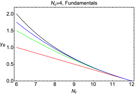
Figure 2: Plot of $\gamma_{B,F,\Delta_{f}^{p}}$ = $\gamma_{\tilde{B},\Delta_{f}^{p}}$ = with $1\leq p\leq 3$, together with the exact $\gamma_{B,F}$, for $G={\rm SU}(4)$ and ${\cal R}=F$, as a function of $N_{f}$, at an IRFP in the non-Abelian Coulomb phase for this theory. For notational simplicity, the vertical axis is labeled simply as $\gamma_{B}$. At $N_{f}=8$, from bottom to top, the curves (with colors online) refer to $\gamma_{B,F,\Delta}$ (red), $\gamma_{B,F,\Delta_{f}^{2}}$ (green), $\gamma_{B,F,\Delta_{f}^{3}}$ (blue), and the exact $\gamma_{B,F}$ (black).

Figure 3: Plot of the exact $\gamma_{M,adj}$ at an IRFP in the non-Abelian Coulomb phase, together with the $O(\Delta_{f}^{p})$ approximations to this result with $1\leq p\leq 3$, for $G={\rm SU}(4)$ and ${\cal R}$ equal to the adjoint representation. From bottom to top, the curves (with colors online) refer to $\gamma_{M,adj,\Delta_{f}}$ (red), $\gamma_{M,adj,\Delta_{f}^{2}}$ (green), $\gamma_{M,adj,\Delta_{f}^{3}}$ (blue), and the exact $\gamma_{M,adj}$ (black).

Figure 4: Plot of the exact $\gamma_{M,S_{2}}$ at an IRFP in the non-Abelian Coulomb phase, together with the $O(\Delta_{f}^{p})$ approximations to this result with $1\leq p\leq 3$, for $G={\rm SU}(3)$ and ${\cal R}=S_{2}$, the symmetric rank-2 tensor representation. From bottom to top, the curves (with colors online) refer to $\gamma_{M,S_{2},\Delta_{f}}$ (red), $\gamma_{M,S_{2},\Delta_{f}^{2}}$ (green), $\gamma_{M,S_{2},\Delta_{f}^{3}}$ (blue), and the exact $\gamma_{M,S_{2}}$ (black).

Figure 5: Plot of the exact $\gamma_{B,S_{2}}$ at an IRFP point in the non-Abelian Coulomb phase, together with the $O(\Delta_{f}^{p})$ approximations to this result with $1\leq p\leq 3$, for $G={\rm SU}(3)$ and ${\cal R}=S_{2}$. From bottom to top, the curves (with colors online) refer to $\gamma_{B,S_{2},\Delta_{f}}$ (red), $\gamma_{B,S_{2},\Delta_{f}^{2}}$ (green), $\gamma_{B,S_{2},\Delta_{f}^{3}}$ (blue), and the exact $\gamma_{B,S_{2}}$ (black).

Figure 7: Plot of the exact $\gamma_{M,A_{2}}$ at an IRFP in the non-Abelian Coulomb phase, together with the $O(\Delta_{f}^{p})$ approximations to this result with $1\leq p\leq 3$, for $G={\rm SU}(5)$ and ${\cal R}=A_{2}$. From bottom to top, the curves (with colors online) refer to $\gamma_{M,A_{2},\Delta_{f}}$ (red), $\gamma_{M,A_{2},\Delta_{f}^{2}}$ (green), $\gamma_{M,A_{2},\Delta_{f}^{3}}$ (blue), and the exact $\gamma_{M,A_{2}}$ (black).

Figure 9: Plot of the exact $\gamma_{B,A_{2}}$ at an IRFP in the non-Abelian Coulomb phase, together with the $O(\Delta_{f}^{p})$ approximations to this result with $1\leq p\leq 3$, for $G={\rm SU}(5)$ and ${\cal R}=A_{2}$. This is the special case of $\gamma_{B,A_{2},Nco}$ in the text for $N_{c}=5$, where the subscript $Nco$ denotes odd $N_{c}$. From bottom to top, the curves (with colors online) refer to $\gamma_{B,A_{2},\Delta_{f}}$ (red), $\gamma_{B,A_{2},\Delta_{f}^{2}}$ (green), $\gamma_{B,A_{2},\Delta_{f}^{3}}$ (blue), and the exact $\gamma_{B,A_{2}}$ (black).