Topological and non inertial effects on the interband light absorption

Abstract

In this work, we investigate the combined influence of the nontrivial topology introduced by a disclination and non inertial effects due to rotation, in the energy levels and the wave functions of a noninteracting electron gas confined to a two-dimensional pseudoharmonic quantum dot, under the influence of an external uniform magnetic field. The exact solutions for energy eigenvalues and wave functions are computed as functions of the applied magnetic field strength, the disclination topological charge, magnetic quantum number and the rotation speed of the sample. We investigate the modifications on the light interband absorption coefficient and absorption threshold frequency. We observe novel features in the system, including a range of magnetic field without corresponding absorption phenomena, which is due to a tripartite term of the Hamiltonian, involving magnetic field, the topological charge of the defect and the rotation frequency.

I Introduction

Quantum dots are often referred to as artificial atoms because of their atom-like electron energy spectrum. They are alluring to a wide range of optoelectronic applications Mohammad Bagher (2016), due to their optical properties, similar to those of atoms Nurmikko (2015). They are able to emit light at specific frequencies if either electricity or light is applied to them. The emitted frequency may be precisely tuned by a careful choice of the size of the dot and/or its shape and composition. In Ref. Tan and Inkson (1996a), an exactly soluble model to describe quantum dots, anti-dots, one-dimensional rings and straight two-dimensional wires in the presence of external fields, was proposed.

An extra ingredient that may influence the tuning of these emission frequencies is a topological defect Katanaev (2005). Defects, in general, are a nuisance since they impair the electronic properties of the materials. Nevertheless, recent works by some of us de Lima and Filgueiras (2012a); de Lima et al. (2013); Bakke and Moraes (2012); Fumeron et al. (2017) have pointed out that topological defects can in fact be used to tailor specific electronic transport properties. Besides the dynamics of carriers, investigations on how topological defects affect the electronic bound states, may also be of importance for the improvement of electronic technology. A step forward in this direction was done in Ref. Filgueiras et al. (2016).

Rotation, as well, has its effects on quantum systems, like in the celebrated Barnett effect Barnett (1915). For instance, in Lima et al. (2014); Lima and Moraes (2015), the low-energy electronic states of rotating fullerene were investigated within a continuum model, motivated by the experimental evidence of rapidly rotating $C_{60}$ molecules in fullerite. In Ref. Fonseca and Bakke (2016), it was shown that rotating effects modify the cyclotron frequency and breaks the degeneracy of the analogue Landau levels for an atom with a magnetic quadrupole moment. The semiclassical kinetic theory of Dirac particles in the presence of external electromagnetic fields and global rotation was established in Dayi et al. (2017). It is clear then, that rotation may be used as an additional tool to manipulate the electronic structure of charge carriers in low dimensional systems as discussed in Filgueiras et al. (2015); Brandao et al. (2015).

As mentioned above, the interband frequency of absorption/emission by a quantum dot can be tuned with slight changes in parameters like size, shape and composition, for instance. In this paper, we add two more ingredients: a topological defect called disclination and rotation. We investigate how the quantum dots and antidots, with the pseudoharmonic interaction and under the influence of external magnetic field, are affected by a combination of non inertial and topological influences. Under these circumstances, we obtain exact analytical expressions for the energy spectrum and wavefunctions of a noninteracting two-dimensional electron gas (2DEG) confined in a quantum dot. The modifications in the light absorption coefficient is examined and the influences in the threshold frequency value of the absorption coefficient are addressed. Separately, rotation Brandao et al. (2015) and disclination Lima et al. (2014) couple to the angular momentum, as does the magnetic field. We will see that, when they act together with a magnetic field on a free 2DEG, a new coupling is found involving all of them simultaneously. This makes the energy levels as function of the magnetic field to bend from the usual straight lines and a range of magnetic field without emission/absorption will be observed.

The plan of this work is the following. In Sec. II, we derive the Schrödinger equation for the 2DEG in a rotating sample, with a disclination, in the presence of an external magnetic field and of a two-dimensional pseudoharmonic potential. Then, we investigate how such physical conditions affect the electronic energy levels. In reality, we consider the 2DEG confined to a flat interface so that we can discuss our results in the context of a (quasi) two-dimensional electron gas. This permits the inclusion of a disclination, since in three-dimensional systems, the very high elastic energy cost forbids the existence of such a defect. In Sec. III, we investigate the modifications due to the topological defect as well as the non inertial effects on the light interband absorption coefficient and absorption threshold frequency. The conclusions are outlined in Section IV.

II The Schrödinger equation for the system

We consider a 2DEG around a disclination, which is a topological defect Katanaev (2005) associated to the removal of a wedge of material with the subsequent identification of the loose ends (Volterra process). This introduces an angular deficit, changing the boundary condition on the angular variable from $\phi\rightarrow\phi+2\pi$ to $\phi\rightarrow\phi+2\pi\alpha$. Here, $\alpha<1$ expresses the removed wedge angle of $2\pi(1-\alpha)$. Conversely, if a wedge is added, $\alpha>1$. This new boundary condition can effectively be incorporated into the theory if we work out in the background space with line element

$$ds^{2}=dr^{2}+\alpha^{2}r^{2}d\phi^{2}+dz^{2}\;.$$ (1)

The topological charge of the defect is given by its Frank vector $f$, which is the curvature flux associated to the defect Katanaev (2005). Since the above line element corresponds to a space with a curvature scalar given by Sátiro et al. (2009)

$$R=2\left(\frac{1-\alpha}{\alpha}\right)\frac{\delta(r)}{r}\;,$$ (2)

its flux is therefore

$$\oint Rrdrd\phi=4\pi\left(\frac{1-\alpha}{\alpha}\right)=f\;.$$ (3)

This result still holds for a two-dimensional surface with a disclination, which is the subject of this article.

The Hamiltonian, in cylindrical coordinates, of a charged particle in a disk rotating with angular velocity $\vec{\Omega}=\Omega\hat{z}$, in the presence of a magnetic field $\vec{B}=B\hat{z}$, can be written as Brandao et al. (2015)

$$H = \frac{[\vec{p}-q\vec{A}-m(\vec{\Omega}\times\vec{r})]^{2}}{2m}-\frac{m(\vec{\Omega}\times\vec{r})^{2}}{2}+$$ (4)

$$+ qV+V_{ext}\;,$$

where $V$ and $\vec{A}$ are the scalar and vector electromagnetic potentials. They are given by

$$V=-\frac{\Omega Br^{2}}{2},$$ (5)

$$\vec{A}=(0,\frac{Br}{2\alpha},0)\;.$$ (6)

The electric field associated to the scalar potential appears from the transformation of the applied magnetic field to the rotating frame. The disclination factor, $\alpha$, appearing in the vector potential compensates the change $\phi\rightarrow\alpha\phi$, giving the correct value of the magnetic flux through a circle of radius $r$ in the plane. That is, $\oint A_{\phi}ds=\oint\frac{Br}{2\alpha}r\alpha d\phi=\pi r^{2}B$, where $ds=\alpha rd\phi$ comes from the metric (1) with $z=const.$, $r=const.$. In the same reasoning, we write the angular momentum operator as $\vec{p}_{\phi}=-\hat{\phi}\frac{i\hbar}{\alpha r}\frac{\partial}{\partial\phi}$.

A scalar pseudoharmonic interaction is incorporated into the system by the potential

$$V_{\mathrm{conf}}=V_{0}\left(\frac{r}{r_{0}}-\frac{r_{0}}{r}\right)^{2},$$ (7)

with $r_{0}=\left(a_{1}/a_{2}\right)^{1/4}$ and $V_{0}$ being the average radius and the chemical potential Ikhdair and Hamzavi (2012), respectively. The choice of the values for the parameters $a_{1}$ and $a_{2}$ specifies the particular system under study, as will be seen below. The model given by Eq. (7) (see also Ref. Tan and Inkson (1996a, b)) was proposed to describe quantum dots, anti-dots, one-dimensional rings and straight two-dimensional wires in the presence of a magnetic field. Some of its properties are: a) the potential (7) has a minimum, $V\left(r\right)=0$, at $r=r_{0}$; b) for $r\rightarrow r_{0}$, the potential of the ring has a parabolic form, $V\left(r\right)\simeq\mu\omega_{0}^{2}\left(r-r_{0}\right)^{2}/2$, with $\omega_{0}=\sqrt{8a_{2}/m}$ being the angular frequency characterizing the strength of the transverse confinement. Another important feature of potential (7) is that we can control its "shape" such that both the radius and the width of the ring can be adjusted independently by suitably choosing $a_{1}$ and $a_{2}$. Then, we can study a $1D$ ring, by choosing $r_{0}=$constant and $\omega_{0}\rightarrow\infty$, a straight 2D wire, by making $\omega_{0}=$constant and $r_{0}\rightarrow\infty$, a quantum dot, by making $a_{1}=0$ and an isolated anti-dot, by making $a_{2}=0$. The particular limits allow us to make a comparison between the electronic states in different geometries.

Including the above contributions, the Hamiltonian is then written as

$$H=\frac{p^{2}}{2m}-\mu rp_{\phi}+\beta r^{2}+\frac{V_{0}r_{0}^{2}}{r^{2}}-2V_{0}\;,$$ (8)

with

$$\mu=\frac{qB}{2m\alpha}+\Omega\\$$ (9)

and

$$\beta = \frac{q^{2}B^{2}}{8m\alpha^{2}}+\frac{qB\Omega}{2}\left(\frac{1-\alpha}{\alpha}\right)+\frac{V_{0}}{r_{0}^{2}}\;.$$ (10)

The $\mu rp_{\phi}$ term contains the usual coupling between the magnetic field and the angular momentum. For this Hamiltonian, the Schrödinger equation can be written as

$$-\frac{\hbar^{2}}{2m}\nabla^{2}\psi + i\frac{\mu\hbar}{\alpha}\frac{\partial\psi}{\partial\phi}+\beta r^{2}\psi+$$ (11)

$$+ \left(\frac{V_{0}r_{0}^{2}}{r^{2}}-2V_{0}\right)\psi=E\psi\;,$$

where the Laplace-Beltrami operator is given by $\nabla^{2}=\frac{\partial^{2}}{\partial r^{2}}+\frac{1}{r}\frac{\partial}{\partial r}+\frac{1}{\alpha^{2}r^{2}}\frac{\partial^{2}}{\partial\phi^{2}}$. With the ansatz $\psi=R(r)e^{-il\phi}$ , Eq. (11) becomes

$$r^{2}R^{\prime\prime}+rR^{\prime}+$$

$$+\left[-\sigma^{2}r^{4}+\gamma r^{2}-\left(\frac{2mV_{0}r_{0}^{2}}{\hbar^{2}}+\frac{\ell^{2}}{\alpha^{2}}\right)\right]R=0,$$ (12)

where $\sigma^{2}=\frac{q^{2}B^{2}}{4\hbar^{2}\alpha^{2}}+\frac{mqB\Omega}{\hbar^{2}}\left(\frac{1-\alpha}{\alpha}\right)+\frac{2mV_{0}}{\hbar^{2}r_{0}^{2}}$, and $\gamma=\frac{2m}{\hbar}\left(\frac{E+2V_{0}}{\hbar}-\frac{qB\ell}{2m\alpha^{2}}-\frac{\Omega\ell}{\alpha}\right)$. Writing $\sigma r^{2}=\xi$ and looking at the asymptotic limits when $\xi\rightarrow\infty$, the general solution to this equation will be given in terms of $\rm M(a,b,\xi)$, which is the confluent hypergeometric function of the first kind Abramowitz and Stegun (1972),

$$R =$$

$$= a_{\ell}e^{-\frac{\xi}{2}}\xi^{\frac{|\ell|}{2\alpha}\Lambda}{\rm M}\left(\frac{-\gamma}{4\sigma}+\frac{|\ell|}{2\alpha}\Lambda+\frac{1}{2},1+\frac{|\ell|}{\alpha}\Lambda,\xi\right)$$

$$+ b_{\ell}e^{-\frac{\xi\Lambda}{2\alpha}}\xi^{-\frac{|\ell|\Lambda}{2\alpha}}{\rm M}\left(\frac{-\gamma}{4\sigma}-\frac{|\ell|}{2\alpha}\Lambda+\frac{1}{2},1-\frac{|\ell|}{\alpha}\Lambda,\xi\right)\;,$$

where $\Lambda=\sqrt{1+\frac{2m\alpha^{2}V_{0}r_{0}^{2}}{\hbar^{2}|\ell|^{2}}}$. In Eq. (LABEL:general_sol_2_HO), $a_{\ell}$ and $b_{\ell}$ are, respectively, the coefficients of the regular and irregular solutions. Notice that the term irregular stems from the fact that this solution diverges as $\xi\rightarrow 0$. We will examine this case since the disclination, described by a cone-like background, introduces a singular potential in the problem Jensen and Dandoloff (2011) associated to the curvature given in Eq. (2). In order to have a finite polynomial function (the hypergeometric series has to be convergent in order to have a physical solution), the condition ${\rm a}=-n$, where $n$ is a positive integer number, must be satisfied. If only the regular solution is to be considered, then $b_{\ell}$ must be zero together with the condition $\frac{|\ell|}{\alpha}\sqrt{1+\frac{2m\alpha^{2}V_{0}r_{0}^{2}}{\hbar^{2}|\ell|^{2}}}\geq 1$. Then, the wave function is square integrable. On the other hand, the constraint $\frac{|\ell|}{\alpha}\sqrt{1+\frac{2m\alpha^{2}V_{0}r_{0}^{2}}{\hbar^{2}|\ell|^{2}}}<1$ must be imposed if the irregular solution is present as a possible wave function. This condition guarantees that it is square integrable Andrade et al. (2013); Khalilov and Mamsurov (2009); Khalilov (2014). From these discussions, the discrete possible values for the energy are given by

$$E = -2V_{0}+\frac{\hbar\omega_{c}\ell}{2\alpha^{2}}+\frac{\hbar\Omega\ell}{\alpha}+$$ (14)

$$+ \hbar\sqrt{\frac{\omega_{c}^{2}}{\alpha^{2}}+4\omega_{c}\Omega\frac{\left(1-\alpha\right)}{\alpha}+\frac{8V_{0}}{mr_{0}^{2}}}\times$$

$$\left[n\pm\frac{1}{2}\sqrt{\frac{\ell^{2}}{\alpha^{2}}+\frac{2mV_{0}r_{0}^{2}}{\hbar^{2}}}+\frac{1}{2}\right],$$

where $\omega_{c}=qB/m$ is the cyclotron frequency. The “$+$” sign stands for the regular wave solution while the “$-$” sign stands for the irregular one. $\vec{B}$ and $\vec{\Omega}$ are tunable external parameters. Considering $\alpha=1$ (flat), $V_{0}=0$ and $\Omega\neq 0$, we recover the results found in Ref. Brandao et al. (2015). By considering $\alpha\neq 1$, $V_{0}=0$ and $\Omega=0$, we recover the results found in Ref. de Lima and Filgueiras (2012b).

III Interband light absorption

In this section, we calculate the direct interband light absorption coefficient $K(\omega)$ and the absorption threshold frequency in a quantum pseudodot under the simultaneous influence of an external magnetic field, rotation and disclination. The light absorption coefficient can be expressed as Atoyan et al. (2004, 2006); Raigoza et al. (2005); Khordad (2010)

$$K(\omega) =N$$

$$\times\sum_{n,l,\mu}\sum_{n^{\prime},l^{\prime},\mu^{\prime}}\left|\int\psi_{n,l,\mu}^{e}\left(r,\phi\right)\psi_{n^{\prime},l^{\prime},\mu^{\prime}}^{h}\left(r,\phi\right)rdrd\phi\right|^{2}$$

$$\times\delta\left(\Delta-E_{n,l,\mu}^{e}-E_{n^{\prime},l^{\prime},\mu^{\prime}}^{h}\right)\;,$$ (15)

where

$$\mu\equiv\pm\sqrt{\frac{|\ell|^{2}}{\alpha^{2}}+\frac{2m_{e}V_{0}r_{0}^{2}}{\hbar^{2}}}\;,$$ (16)

$$\mu^{\prime}\equiv\pm\sqrt{\frac{|\ell|^{2}}{\alpha^{2}}+\frac{2m_{h}V_{0}r_{0}^{2}}{\hbar^{2}}}\;,$$ (17)

$\Delta\equiv\hbar\varpi-\varepsilon_{g}$, $\varepsilon_{g}$ is the width of the forbidden energy gap, $\varpi$ is the frequency of incident light, $N$ is a quantity proportional to the square of dipole moment matrix element modulus, $\psi^{e\left(h\right)}$ is the wave function of the electron (hole) and $E^{e(h)}$ is the corresponding energy of the electron (hole). Considering the solution (LABEL:general_sol_2_HO), Eq.(15) becomes Ikhdair and Hamzavi (2012)

$$K(\omega) =N\sum_{n,l,\mu}\sum_{n^{\prime},l^{\prime},\mu^{\prime}}\frac{\sigma^{\mu+\mu^{\prime}+2}(n+\mu)!(n^{\prime}+\mu^{\prime})!}{\pi^{2}n!n^{\prime}!\left(\left|\mu\right|!\right)^{2}(\left|\mu^{\prime}\right|!)^{2}}$$

$$\times\Bigg{|}\int_{0}^{2}\pi e^{i(l+l^{\prime})}\int_{0}^{\infty}rdre^{-\frac{1}{2}(\sigma+\sigma^{{}^{\prime}})r^{2}}r^{\mu+\mu^{\prime}}$$

$$\times\,\mathrm{M}\left(-n,1+\mu,\sigma r^{2}\right)\mathrm{M}\left(-n^{\prime},1+\mu^{\prime},\sigma^{\prime}r^{2}\right)\Bigg{|}^{2}$$

$$\times\,\delta\left(\Delta-E_{n,l,\mu}^{e}-E_{n^{\prime},l^{\prime},\mu^{\prime}}^{h}\right)\;.$$ (18)

Following Ref. Ikhdair and Hamzavi (2012), the light absorption coefficient is given by

$$K\left(\omega\right)=N\sum_{n,l,\mu}\sum_{n^{\prime},l^{\prime},\mu^{\prime}}P_{nn^{\prime}}^{\mu}Q_{nn^{\prime}}^{\mu}\delta\left(\Delta-E_{n,l,\mu}^{e}-E_{n^{\prime},l^{\prime},\mu^{\prime}}^{h}\right)\;,$$ (19)

where

$$P_{nn^{{}^{\prime}}}^{\mu} =\frac{1}{\left(\mu!\right)^{4}}(\sigma\sigma^{\prime})^{\mu+1}\left(\frac{\sigma+\sigma^{\prime}}{\sigma-\sigma^{\prime}}\right)^{2\left(n+n^{\prime}\right)}$$

$$\times\frac{\left(n+\mu\right)!\left(n^{\prime}+\mu\right)!}{n!n^{\prime}!}\;,$$

and

$$Q_{nn^{\prime}}^{\mu}=\left[A_{\mu,\sigma}\mathrm{M}\left(n,n^{\prime},\mu+1;-\frac{4\sigma\sigma^{\prime}}{\left(\sigma-\sigma^{\prime}\right)^{2}}\right)\right]^{2},$$

where

$$A_{\mu,\sigma}=\left(\lvert\mu\rvert\right)!\left(\frac{2}{\sigma+\sigma^{\prime}}\right)^{2\mu+1}\;.$$

The argument of the Dirac delta function in Eq. (19) together with Eq. (14), allows us to define the absorption threshold frequency as

$$\hbar\varpi = \varepsilon_{g}+\left[\hbar\left(n+\frac{\mu}{2}+\frac{1}{2}\right)\Xi_{e}+\frac{\hbar\ell}{2\alpha}\left(-\frac{\omega_{ce}}{\alpha}+2\Omega\right)\right]+$$

$$+ \left[\hbar\left(n^{\prime}+\frac{\mu^{\prime}}{2}+\frac{1}{2}\right)\Xi_{h}+\frac{\hbar\ell^{\prime}}{2\alpha}\left(\frac{\omega_{ch}}{\alpha}+2\Omega\right)\right]-4V_{0},$$

where

$$\Xi_{e}=\sqrt{\frac{\omega_{ce}^{2}}{\alpha^{2}}-4\omega_{ce}\Omega\frac{(1-\alpha)}{\alpha}+\frac{8V_{0}}{m_{e}r_{0}^{2}}}\;,$$ (21)

for electrons, and

$$\Xi_{h}=\sqrt{\frac{\omega_{ch}^{2}}{\alpha^{2}}+4\omega_{ch}\Omega\frac{(1-\alpha)}{\alpha}+\frac{8V_{0}}{m_{h}r_{0}^{2}}}\;,$$ (22)

for holes. In these equations, $\omega_{ce}=eB/m_{e}$ and $\omega_{ch}=eB/m_{h}$, where $e$ is the elementary charge and $m_{e}$ and $m_{h}$ are, respectively, the effective masses of the electron and the hole.

Let us now investigate the influence a disclination ($\alpha$) as well as rotation ($\Omega$) on the threshold value of the absorption for the transition $00\rightarrow 00$, comparing with the case where these ingredients are absent. The threshold value of absorption is then given by

$$\hbar\varpi_{00} = \varepsilon_{g}+\left[\hbar\left(\pm\sqrt{\frac{m_{e}V_{0}r_{0}^{2}}{2\hbar^{2}}}+\frac{1}{2}\right)\Xi_{e}\right]$$ (23)

$$+ \left[\hbar\left(\pm\sqrt{\frac{m_{h}V_{0}r_{0}^{2}}{2\hbar^{2}}}+\frac{1}{2}\right)\Xi_{h}\right]-4V_{0}.$$

From Eq. (23), we can define the dimensionless absorption threshold as

$$W=\frac{\hbar\varpi_{00}}{\varepsilon_{g}}.$$ (24)

For a quantum dot $(V_{0}r_{0}^{2}\rightarrow 0)$, we obtain the absorption threshold frequency as

$$W=1+\frac{\hbar}{2\varepsilon_{g}}(\Xi_{e}+\Xi_{h})-\frac{4V_{0}}{\varepsilon_{g}}.$$ (25)

Before analyzing the consequences of Eq. (25) we note that the second term in the square root in Eqs. (21) and (22) is proportional to the product $eB\Omega f$, where the topological charge $f$ is given by Eq. (3). This remarkable term shows how the electric charge of the carrier, the magnetic field strength, the rotation speed and the topological charge of the disclination couple as a simple product. This has profound implications in the absorption threshold since it is sensitive to the signs of each one of them. So, whether the carrier is an electron or a hole, or whether $\vec{B}$ and $\vec{\Omega}$ are parallel or anti-parallel, or whether the disclination has negative or positive curvature, it all matters. Whatever the combination of signs entering the product, the sign in front of the corresponding terms in Eqs. (21) and (22) will always be opposite. This implies that, in some cases, either equation might yield imaginary results which indicate that there are no bound states in these conditions (see Eq. (14)). This explains the sudden stop of two of the curves in Fig. 2 below.

In Fig. 1, we show the absorption threshold frequency $W$ versus magnetic field $B$, for different values of $\alpha$ and of $\Omega$. In Fig. 1(a) it can be observed that for any disclination $\alpha$ and angular frequency $\Omega$, the behavior is linear for strong applied magnetic fields. One can also see that, for a positive curvature disclination ($\alpha<1$), the frequency increases faster than in the negative curvature disclination ($\alpha>1$) case. On the other hand, in Fig. 1(b) one can see that, for weak magnetic fields, the absorption threshold frequency is nonlinear. Furthermore, it is seen that an increase of the angular frequency from $\Omega=0$ (red dashed line) to $\Omega=500$ Ghz (red solid line) rises the absorption threshold frequency $W$ for $\alpha=\frac{5}{6}$ and $B>0$, while for $B<0$, the effect is opposite. Also, we can see that, increasing the angular frequency $\Omega=0$ (blue dashed line) to $\Omega=500$ Ghz (blue solid line), lowers the absorption threshold frequency for $\alpha=\frac{7}{6}$ and $B>0$. In the region $B<0$ the effect is opposite. Finally, when the system has no disclination ($\alpha=1$), the threshold frequency is independent of $\Omega$ (the solid and the dashed line coincide).

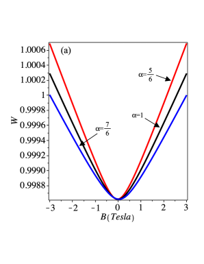
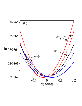
Figure 1: (Color online) The absorption threshold frequency $W$ as a function of magnetic field $B$ for $\Omega=500$ Ghz (solid lines), $\Omega=0$ Ghz (dashed lines) and three values of the disclination parameter $\alpha$: (a) strong magnetic field and (b) weak magnetic field. The quantum dot size $r_{0}=895.8$ $\mathring{A}$ was assumed for all plots.

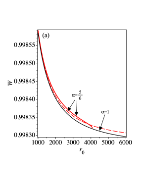
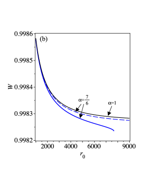
Figure 2: (Color online) The absorption threshold frequency $W$ versus quantum dot size $r_{0}$ (in $\mathring{A}$) for $B=0.1T$ (all lines) and $\Omega=0$ (dashed lines), $\Omega=500$ Ghz (solid lines): (a) $\alpha=5/6$ and (b) $\alpha=7/6$. The $\alpha=1$, or defectless case (solid black line), which does not depend on $\Omega$, is also plotted for comparison. Notice the abrupt ending of the colored solid lines in both cases.

In Fig. 2, we present plots of the absorption threshold frequency as a function of the quantum dot size $r_{0}$ (in $\mathring{A}$) for $\Omega=0$, $\Omega=500$ Ghz, $B=0.1T$ and a few values of the disclination parameter $\alpha$. As seen from the figures, the absorption threshold frequency decreases with the increasing of the quantum dot radius in all cases. In Fig. 2(a), we note that the threshold frequency decreases monotonically for $\alpha=1$ (black solid line), $\alpha=\frac{5}{6}$ (red solid line), both of these at $\Omega=500$ GHz. Same behavior for the $\Omega=0$ case. Moreover, we find that the threshold frequency decreases monotonically but suddenly disappears in the case of the disclination assuming the value $\alpha=\frac{5}{6}$ (red solid line) and $\Omega=500$ GHz. Fig. 2(b) shows that the curve of the absorption threshold frequency shifts down when the disclination parameter changes from $\alpha=1$ (black solid line) to $\alpha=\frac{7}{6}$ (blue dashed line). One interesting observation is that the absorption threshold frequency suddenly disappears for disclination parameter $\alpha=\frac{7}{6}$ (blue solid line) and $\Omega=500$ GHz. As mentioned above, the abrupt ending of the curves in Fig. 2 is due to the absence of bound states in the region beyond. That is, for a given disclination, for fixed values of $B$ and $\Omega$, there is an upper limit for the radius of the quantum dot. This is clear if one takes a look at the Hamiltonian (8). If $\beta$, as given by Eq. (10), becomes negative, clearly, the effective potential in (8) does not yield bound states.

In Fig. 3, we investigate the effect of the angular frequency $\Omega$ on the absorption threshold frequency $W$ for magnetic field $B=0.1T$ and $B=3T$, and also for three different values of the disclination parameter $\alpha$. First, it can be seen from Fig. 3(a), where $B=0.1T$, that when $\alpha=\frac{5}{6}$ (a wedge is removed), the maximum of the absorption frequency corresponds to an anticlockwise (positive) angular velocity $\Omega$ and it decreases with increasing $\Omega$ until it suddenly disappears. Furthermore, for clockwise (negative) angular velocity, the absorption frequency continues to decrease as $|\Omega|$ increases. In the case where $\alpha=\frac{7}{6}$ (a wedge is added), the figure shows a nearly symmetric behavior with the threshold frequency increasing when anticlockwise angular velocity decreases. On the other hand, in the region of clockwise angular velocity the threshold frequency increases with increasing $|\Omega|$ until it reaches the maximum peak. Soon after this, it suddenly disappears. Finally, when the system has no disclination, $\alpha=1$, the threshold frequency absorption is independent of the angular frequency.

As shown in Fig. 3(b) for $B=3T$, the gap between the threshold frequency maximum for $\alpha=\frac{5}{6}$ and $\alpha=\frac{7}{6}$ is greater than in case $B=0.1T$. The stronger magnetic field has moved the $W(\Omega)$ curves with respect to each other as compared to Fig. 3. Now the $\alpha=\frac{5}{6}$ and $\alpha=\frac{7}{6}$ no longer cross each other.

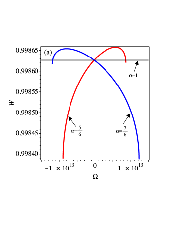
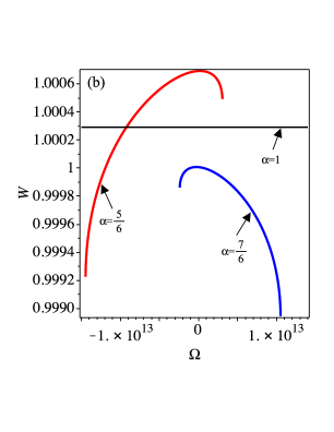
Figure 3: (Color online) The absorption threshold frequency $W$ as a function of angular frequency $\Omega$ for $\alpha=\frac{5}{6}$, $\alpha=1$, $\alpha=\frac{7}{6}$. (a) $B=0.1T$. (b) $B=3T$. The quantum dot size $r_{0}=895.8$ $\mathring{A}$ was assumed for all plots.

When we consider the quantum anti-dot $\left(\frac{V_{0}}{r_{0}^{2}}\rightarrow 0\right)$, the absorption threshold frequency is given by the expression

$$W=1-\frac{4V_{0}}{\varepsilon_{g}}+\frac{\hbar}{2\varepsilon_{g}}\left[\Phi_{e}\left(1+\sqrt{\frac{2m_{e}V_{0}r_{0}^{2}}{\hbar^{2}}}\right)+\right.$$

$$\left.+\Phi_{h}\left(1+\sqrt{\frac{2m_{h}V_{0}r_{0}^{2}}{\hbar^{2}}}\right)\right]\;,$$ (26)

where $\Phi_{e(h)}=\sqrt{\frac{\omega_{ce(h)}^{2}}{\alpha^{2}}\pm 4\omega_{ce(h)}\Omega\frac{(1-\alpha)}{\alpha}}$.

Fig. 4 shows the variation of the absorption threshold frequency $W$ for a quantum anti-dot as a function of the magnetic field $B$, for fixed $\Omega=0$, $\Omega=500$ Ghz and different values of the disclination parameter $\alpha$. As illustrated in Fig. 4(a) the behavior of the threshold frequency is linear for strong magnetic fields for $\alpha=\frac{5}{6}$ (red solid line), $\alpha=1$ (black solid line), $\alpha=\frac{7}{6}$ (blue solid line) and independent of the values of $\Omega$. On the other hand, in Fig. 4(b), we show the magnetic field dependence of the threshold frequency for small magnetic fields. The results show clearly that for $\Omega=0$, the behavior of the threshold frequency, for several values of parameter $\alpha$, is linear. However, the most striking finding happens when angular velocity is not null (here, we consider $\Omega=500$ Ghz) for $\alpha=\frac{5}{6}$ (red solid lines) and $\alpha=\frac{7}{6}$ (blue solid lines) it is found that, in the weak magnetic field region the threshold frequency suddenly disappears. Again, the reason is the absence of bound states due an imaginary value of $\beta$.

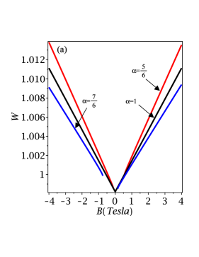
Figure 4: (Color online) The absorption threshold frequency $W$ for a quantum anti-dot as a function of magnetic field $B$, for several values of the disclination parameter $\alpha$ and for $\Omega=500$ Ghz. (a) strong magnetic field. (b) weak magnetic field. The quantum anti-dot size $r_{0}=895.8$ $\mathring{A}$ was assumed for all plots.

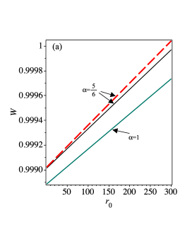
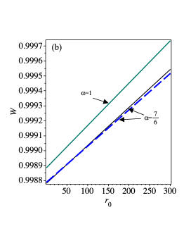
Figure 5: (Color online) The absorption threshold frequency $W$ versus quantum anti-dot size $r$ for the fixed value $B=1T$. (a) For $\alpha=\frac{5}{6}$ with $\Omega=500$ GHz (black line), $\Omega=0$ (red dashed line) and $\alpha=1$ with $\Omega=500$ GHz (green line). (b) For $\alpha=\frac{7}{6}$ with $\Omega=500$ GHz (black line), $\Omega=0$ (blue dashed line). The green line corresponds to $\alpha=1$ with $\Omega=500$ GHz.

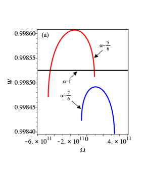
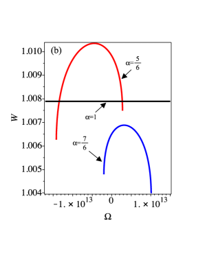
Figure 6: (Color online) The absorption threshold frequency $W$ for a quantum anti-dot as a function of angular frequency $\Omega$, for several values of the disclination parameter $\alpha$. (a) $B=0.1T$. (b) $B=3T$. The quantum anti-dot size $r_{0}=895.8$ $\mathring{A}$ was assumed for all plots.

In Fig. 5, we plot the absorption threshold frequency $W$ as a function of the quantum anti-dot radius $r_{0}$ for $B=1T$. From Fig. 5(a), we see that the behavior of $W$ is linear for $\alpha=\frac{5}{6}$ and $\alpha=1$. One interesting observation is that the presence of the positive disclination ($\alpha=\frac{5}{6}$) shifts up the threshold frequency. In Fig. 5(b) we give the plot of $W$ as a function of radius $r_{0}$. One can be observe that when we have negative disclination ($\alpha=\frac{7}{6}$) the behavior of the $W$ is linear. And is always less than $\alpha=1$, when the system has no disclination.

In Fig. 6, we plot of the threshold frequency $W$ as a function of the angular frequency $\Omega$ for different values of the magnetic fields $B$ and disclination parameter $\alpha$ for the quantum anti-dot. As shown in Fig. 6(a), the intensity of the absorption threshold frequency for $\alpha=\frac{5}{6}$ is higher than in the case $\alpha=\frac{7}{6}$ in the regime of the weak magnetic field ($B=0.1T$). One also can see that the behavior is different from the one shown in Fig. 3(a) above, since there is no crossing between the threshold frequency curves corresponding to the disclination parameters $\alpha=\frac{5}{6}$ and $\alpha=\frac{7}{6}$. Finally, Fig. 6(b) describes the behavior of the threshold frequency for $B=3T$. In this case, as seen from the plots, the intensity of the absorption threshold frequency is higher than in the case for weak magnetic field ($B=0.1T$).

IV Conclusion

We have investigated the energy levels of a 2DEG in the presence of a disclination, under the influence of a pseudoharmonic interaction consisting of either a quantum dot or an antidot potential, in the presence of a strong uniform magnetic field $B$, in a rotating sample. The topological defect generates a curvature field that acts on the particles as an external AB flux. We have considered the effects of a covariant term, which comes from the geometric approach in the continuum limit. This is due to elastic deformations in the material with such disclination. We have found that this changes significantly the interband light absorption in this system. Moreover, we have seen that there is a simultaneous coupling between rotation, magnetic field and the topological defect which gives rise to a range of values for the magnetic field that does not exhibit absorption of light. This is due to the fact that there is no binding of electrons in this range. The size of this region depends on the disclination and the rotation rate. It also depends on which material is being considered trough the effective mass of the charge carriers. The most important feature of this effect is that it only exists when the three elements (magnetic field, disclination and rotation) are present simultaneously.