Dynamical gluon mass in the instanton vacuum model

Abstract

We consider the modifications of gluon properties in the instanton liquid model (ILM) for the QCD vacuum. Rescattering of gluons on instantons generates the dynamical momentum-dependent gluon mass $M_{g}(q).$ First, we consider the case of a scalar gluon, no zero-mode problem occurs and its dynamical mass $M_{s}(q)$ can be found. Using the typical phenomenological values of the average instanton size $\rho=1/3\,\,fm$ and average inter-instanton distance $R=1\,\,fm$ we get $M_{s}(0)=256\,\,MeV$. We then extend this approach to the real vector gluon with zero-modes carefully considered. We obtain the following expression $M^{2}_{g}(q)=2M^{2}_{s}(q).$ This modification of the gluon in the instanton media will shed light on nonperturbative aspect on heavy quarkonium physics.

I Introduction

Without any doubt instantons represent a very important topologically nontrivial component of the QCD vacuum. The main parameters of the QCD instanton vacuum developed in the instanton liquid model (ILM) are the average instanton size $\rho$ and inter-instanton distance $R$ (see, for example, following reviews Diakonov (2003); Schafer and Shuryak (1998)). They were phenomenologically estimated as $\rho=1/3\,\mathrm{fm},\,R=1\,\mathrm{fm}$ and confirmed by theoretical variational calculations Diakonov (2003); Schafer and Shuryak (1998) and recent lattice simulations of the QCD vacuum Chu et al. (1994); Negele (1999); DeGrand (2001); Faccioli and DeGrand (2003); Bowman et al. (2004). In particular, the spontaneous breakdown of chiral symmetry is realized very well via the ILM Goeke et al. (2007). Hence, instantons play a pivotal and significant role in describing the lightest hadrons and their interactions.

In the ILM the instanton induces strong interactions between light quarks and produce a large dynamical mass $M$, which was initially almost massless. Consequently, light quarks are bound and the pions as a pseudo-Goldstone boson appear as a result of spontaneous breakdown of chiral symmetry (SBCS).

On the other hand, the instantons from the QCD vacuum also interact with heavy quarks and are responsible for the generation of the heavy-heavy and heavy-light quark interactions with trace of the SBCS Musakhanov (2012, 2015, 2017). It is important to note that the packing parameter is given as $\rho^{4}/R^{4}$ and it become very small ($\sim 0.01$) with the phenomenological values of $\rho$ and $R$ used. Then, the dynamical quark mass $M$ is expressed as $(packing\,\,parameter)^{1/2}\rho^{-1}\sim 365$ MeV Diakonov (2003) while the instanton contribution to the heavy quark mass is given as $\Delta M\sim(packing\,\,parameter)\rho^{-1}\sim 70$ MeV Diakonov et al. (1989). We see that these specific $packing\,\,parameter$ dependencies explain the values of $M$ and $\Delta M$. These factors define the coupling between the light-light, heavy-light and heavy-heavy quarks induced by the instantons from the QCD vacuum.

The direct instanton effects mainly contribute to the intermediate region characterized by the instanton size ($\rho\simeq 0.33$ fm), as was studied in Ref. Yakhshiev et al. (2017) in which the instanton effects are marginal but still important to be considered for a quantitative description of the heavy quarkonium spectra. One-gluon exchange is dominant at smaller distances. On the other hand, a size of the heavy quarkonium is small Digal et al. (2005). It means that heavy quarkonium properties might be sensitive to a modification of gluon properties in instanton media (ILM) induced by rescattering of gluons on the instantons.

Previously the dynamical gluon mass $M_{g}$ within ILM was estimated in Hutter (1995) as $M_{g}\sim 400\,MeV$ with phenomenological values of $\rho$ and $R$. However, this estimation was obtained by ignoring the gluon zero-modes problem and some $SU(N_{c})$ factors.

In this work, we aim at investigating the dynamical gluon mass within the ILM, extending the method developed in Ref. Pobylitsa (1989), where the formulae for the quark correlators were derive.

II Scalar ”gluon” propagator

We start from the scalar massless field $\phi$ belonging to the adjoint representation as a real gluon. We have to find its propagator in the external classical gluon field in the ILM $A_{\mu}=\sum_{I}A^{I}_{\mu}(\gamma_{I})$, where $A^{I}_{\mu}(\gamma_{I})$ is a generic notation for the QCD (anti-) instanton in the singular gauge. $\gamma_{I}$ stands for all the relevant collective coordinates: the position in Euclid 4D space $z_{I}$, the size $\rho_{I}$ and the $SU(N_{c})$ color orientation $U_{I}$. The number of the collective coordinates is $4N_{c}$.

The action is defined as $S_{\phi}=(\phi^{+}P^{2}\phi)$ where $P_{\mu}=p_{\mu}+A_{\mu}$ (in the coordinate representation $p_{\mu}=i\partial_{\mu}$). The scalar gluon-like propagator is given by

$$\Delta=(p+A)^{-2}=(p^{2}+\sum_{i}(\{p,A_{i}\}+A_{i}^{2})+\sum_{i\neq j}A_{i}A_{j})^{-1},\,\,\,\Delta_{0}=p^{-2},$$ (1)

$$\tilde{\Delta}=(p^{2}+\sum_{i}(\{p,A_{i}\}+A_{i}^{2}))^{-1},\,\,\,\,\Delta_{i}=P_{i}^{-2}=(p^{2}+\{p,A_{i}\}+A_{i}^{2})^{-1}.$$

There are no zero modes in $\Delta^{-1}_{i}=P_{i}^{2}$ and $\Delta^{-1}=P^{2}$, which means the existence of the inverse operators $\Delta_{i}$ and $\Delta$. Our aim is to find the propagator averaged over instanton collective coordinates $\bar{\Delta}\equiv<\Delta>=\int D\gamma\,\Delta.$ However, we start first from $\bar{\tilde{\Delta}}.$ Expanding $\tilde{\Delta}$ over $(\{p,A_{i}\}+A_{i}^{2})$ carrying out further resummation, we obtain the multi-scattering series

$$\tilde{\Delta}=\Delta_{0}+\sum_{i}(\Delta_{i}-\Delta_{0})+\sum_{i\neq j}(\Delta_{i}-\Delta_{0})\Delta_{0}^{-1}(\Delta_{j}-\Delta_{0})+...$$ (2)

As in Ref. Pobylitsa (1989), the main contribution to the $\bar{\tilde{\Delta}}$ can be summed up by the following equation

$$\bar{\tilde{\Delta}}-\Delta_{0}=\sum_{i}<\{{\bar{\tilde{\Delta}}}^{-1}(\Delta_{0}^{-1}-\Delta_{i}^{-1})^{-1}\Delta_{i}^{-1}-(\Delta_{0}^{-1}-{\bar{\tilde{\Delta}}}^{-1})\}^{-1}>$$ (3)

Rewriting this equation, we have

$$\bar{\tilde{\Delta}}^{-1}-\Delta_{0}^{-1}=\sum_{i}<\{\bar{\tilde{\Delta}}+(\Delta_{i}^{-1}-\Delta_{0}^{-1})^{-1}\}^{-1}>$$ (4)

We can derive the solution of Eqs. (3) and (4) in the ILM by expanding with respect to the instanton density $N/V=1/R^{4}$, since the actual dimensionless expansion parameter is in fact the packing parameter $\rho^{4}/R^{4}$. The solution of Eq. (4) in the first-order expansion with respect to the density comes from the iteration if replaces the right-hand side of this equation by $\bar{\tilde{\Delta}}\rightarrow\Delta_{0}$. Then we have

$$\bar{\tilde{\Delta}}^{-1}-\Delta_{0}^{-1} = <\sum_{i}\{\Delta_{0}+(\Delta_{i}^{-1}-\Delta_{0}^{-1})^{-1}\}^{-1}>$$ (5)

$$= -<\sum_{i}\Delta_{0}^{-1}(\Delta_{i}-\Delta_{0})\Delta_{0}^{-1}>=N\Delta_{0}^{-1}(\bar{\Delta}_{I}-\Delta_{0})\Delta_{0}^{-1},$$

where $\bar{\Delta}_{I}=\int d\gamma_{I}\,\Delta_{I}$. Now we compare $\Delta$ with $\tilde{\Delta}$. Expanding $\Delta$ with respect to $A_{i}A_{j}$, we get

$$\Delta=\tilde{\Delta}-\tilde{\Delta}\sum_{i\neq j}A_{i}A_{j}\Delta=\tilde{\Delta}-\tilde{\Delta}\sum_{i\neq j}A_{i}A_{j}\tilde{\Delta}+...$$ (6)

It means immediately $\bar{\Delta}-\bar{\tilde{\Delta}}=O(N^{2})$ which is negligible. We have to take a well-known results for $\Delta_{I}$ from Ref. Brown et al. (1978):

$$\Delta^{ab}_{I}=\frac{1}{2}{\rm tr}\frac{\tau_{a}F(x,y)\tau_{b}F(y,x)}{4\pi^{2}(x-y)^{2}\Pi(x)\Pi(y)},\,\,\,\,\Pi(x)=\frac{x^{2}+\rho^{2}}{x^{2}},$$ (7)

$$\tau_{\mu}=(\vec{\tau},i),\,\,\,\tau^{+}_{\mu}=(\vec{\tau},-i),\,\,\,\tau_{\mu}\tau^{+}_{\nu}=\delta_{\mu\nu}+i\bar{\eta}_{a\mu\nu}\tau_{a},$$ (8)

$$F(x,y)=1+\rho^{2}\frac{(\tau x)(\tau^{+}y)}{x^{2}y^{2}}=1+\rho^{2}\frac{(xy)}{x^{2}y^{2}}+\rho^{2}\frac{i\bar{\eta}_{a\mu\nu}\tau_{a}x_{\mu}y_{\nu}}{x^{2}y^{2}},$$ (9)

where $\bar{\eta}_{a\mu\nu}=-\bar{\eta}_{a\nu\mu}$ is the ’tHooft symbol. We assume that the position of the instanton $z=0$ and the orientation $U=1$. It is clear to see from Eq. (5) that the gluon-like scalar dynamical mass operator is given by

$$M_{s}^{2}\delta_{ab}=<\sum_{i}p^{2}(\Delta^{ab}_{i}-\Delta^{ab}_{0})p^{2}>=N(p^{2}\bar{\Delta}^{ab}_{I}p^{2}-\delta_{ab}p^{2}).$$ (10)

In order to average over the position $z$, we have to change $x\rightarrow x-z$, $y\rightarrow y-z$ and perform integration $\int d^{4}z$. Similarly, we average over the color orientation $U$. Introducing the orientation factor $O^{ab}={\rm tr}(U^{+}t^{a}U\tau^{b})$, where $t_{a}$ are $SU(N_{c})$- matrices, we change $\Delta^{ab}_{I}$ to be $O^{ab}O^{a^{\prime}b^{\prime}}\Delta^{bb^{\prime}}_{I}$, and carry out integration $\int dO$. Here $\int dOO^{ab}O^{ab^{\prime}}=\delta_{bb^{\prime}},\int dOO^{ab}O^{a^{\prime}b^{\prime}}=(N_{c}^{2}-1)^{-1}\delta_{aa^{\prime}}\delta_{bb^{\prime}}$. Also, $\int dOO^{ab}\bar{\eta}_{b\mu\nu}O^{a^{\prime}b^{\prime}}\bar{\eta}_{b^{\prime}\mu^{\prime}\nu^{\prime}}=(N_{c}^{2}-1)^{-1}\delta_{aa^{\prime}}(\delta_{\mu\mu^{\prime}}\delta_{\nu\nu^{\prime}}-\delta_{\mu\nu^{\prime}}\delta_{\nu\mu^{\prime}}).$ In coordinate space, we find

$$\bar{\Delta}^{aa^{\prime}}_{I}(x,y)-\Delta^{aa^{\prime}}_{0}(x,y)$$

$$=\int d^{4}zdOO^{ac}O^{a^{\prime}c^{\prime}}(\Delta^{cc^{\prime}}_{I}(x^{\prime},y^{\prime})-\Delta^{cc^{\prime}}_{0}(x^{\prime},y^{\prime}))\,\,\,(x^{\prime}\equiv x-z,\,\,\,y^{\prime}\equiv y-z),$$

$$=\delta_{aa^{\prime}}\int d^{4}z[\frac{3\rho^{2}}{4\pi^{2}(N_{c}^{2}-1)}f_{1}(x^{\prime})f_{1}(y^{\prime})+\frac{2\rho^{4}}{N_{c}^{2}-1}f_{2}(x^{\prime})g(x^{\prime}-y^{\prime})f_{2}(y^{\prime})],$$ (11)

$$f_{1}(x)=\frac{1}{(x^{2}+\rho^{2})},\,\,\,f_{2}(x)=\frac{(x_{\mu}x_{\nu},ix^{2})}{x^{2}(x^{2}+\rho^{2})},\,\,\,\,g(x-y)=\frac{1}{4\pi^{2}(x-y)^{2}}.$$

In momentum space, we find the contribution from the first term in Eq. (11) as

$$M_{1,s}(q)=[\frac{3\rho^{2}}{(N_{c}^{2}-1)R^{4}}4\pi^{2}]^{1/2}q\rho K_{1}(q\rho)$$ (12)

where the form factor $q\rho K_{1}(q\rho)$. $K_{1}$ denotes the modified Bessel function. In Fig. 1, we draw the form factor.

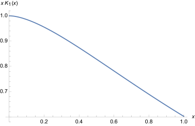
Figure 1: Scalar ”gluon” dynamical mass form-factor as a function of $x=q\rho$.

The estimation of the contribution from the second term in Eq. (11) leads to $M_{2,s}(0)=0$, while in general we know $M_{2,s}(q\rightarrow\infty)\rightarrow 0.$ It means that we may neglect this contribution at all and obtain $M_{s}(q)=M_{1,s}(q)$. Using the phenomenological values of $\rho$ and $R$, we obtain $M_{s}(0)=256\,MeV$.

III Real gluon propagator

The total gluon field in the ILM is $A+a$, where $A=\sum_{i}A^{i}(\gamma_{i})$. The number of all collective coordinates $\gamma_{i}$ is equal to $4N_{c}N$. We have to decompose the so-called zero modes $\phi_{\mu}^{i}$ from the total fluctuation $a$, which are the fluctuations along the collective coordinates $\gamma_{i}$ in the functional space. Consider first the single instanton case, based on Refs. Vandoren and van Nieuwenhuizen (2008); Brown and Lee (1978). All of the fluctuations will be taken with gauge fixing condition $P^{I}_{\mu}a_{\mu}=0$ imposed. Then, the quadratic part of the effective action is given as $(a_{\mu}M^{I}_{\mu\nu}a_{\nu})$, where $M^{I}_{\mu\nu}={P^{I}}^{2}\delta_{\mu\nu}+2iG^{I}_{\mu\nu}-(1-1/\xi)P^{I}_{\mu}P^{I}_{\nu}$ and $G^{I}_{\mu\nu}=-i[P^{I}_{\mu},P^{I}_{\nu}]$. Here $\xi$ stands for the gauge fixing parameter. The zero modes are the solutions of the following equation

$$M^{I}_{\mu\nu}\phi^{i}_{\nu}=0.$$ (13)

In some sense the zero modes can be considered as derivatives with respect to collective coordinates of the instanton field together with the additional longitudinal term dictated by the gauge fixing condition. The projection operator to the instanton zero-modes space is defined as $P^{I}_{\mu\nu}=\sum_{i}\phi^{i}_{\mu}\phi^{i+}_{\nu}$, while that to the nonzero modes space is defined as $Q^{I}_{\mu\nu}=\delta_{\mu\nu}-P^{I}_{\mu\nu}.$ The gluon propagator $S^{I}_{\mu\nu}$ is defined by the following equation

$$M^{I}_{\mu\nu}S^{I}_{\nu\rho}=Q^{I}_{\mu\rho}$$ (14)

The explicit solution of this equation was already derived in Ref. Brown et al. (1978). To generalize the formulae in Ref. Pobylitsa (1989), we introduce an artificial gluon mass $m$,which will be taken zero at the end of calculation. So, we define $g^{I}_{m,\mu\nu}$ and take the limit of $\lim_{m\rightarrow 0}g^{I}_{m,\mu\nu}=S^{I}_{\mu\nu},$ where

$$(M^{I}_{\mu\rho}+m^{2}\delta_{\mu\rho})g^{I}_{m,\rho\nu}=Q^{I}_{\mu\nu}.$$

We also introduce $G^{I}_{m,\rho\nu}$, satisfying

$$(M^{I}_{\mu\rho}+m^{2}\delta_{\mu\rho})G^{I}_{m,\rho\nu}=\delta_{\mu\nu}.$$

As was shown in Ref. Brown and Lee (1978), we find

$$G^{I}_{m,\rho\nu}=g^{I}_{m,\rho\nu}+\frac{1}{m^{2}}P^{I}_{\rho\nu}.$$

It is clear to see that

$${G^{I}}^{-1}_{m,\mu\rho}=(M^{I}_{\mu\rho}+m^{2}\delta_{\mu\rho}).$$

Now we may repeat the the same method with which we are able to obtain the averaged ILM ”scalar” gluon propagator $\bar{\tilde{\Delta}}$ given in Eqs. (3,4). First, we introduce the ILM inverse massive gluon propagator

$${G}^{-1}_{m,\mu\rho}={P}^{2}\delta_{\mu\nu}+2iG_{\mu\nu}+m^{2}\delta_{\mu\rho}=\tilde{M}_{\mu\nu}+m^{2}\delta_{\mu\rho}+\sum_{i\neq j}(A^{i}A^{j}\delta_{\mu\nu}-i[A^{i}_{\mu},A^{j}_{\nu}]).$$

and

$$\tilde{G}^{-1}_{m,\mu\nu}=\tilde{M}_{\mu\nu}+m^{2}\delta_{\mu\nu}=p^{2}+\sum_{i}((\{p,A^{i}\}+{A^{i}}^{2})\delta_{\mu\nu}+2iG^{i}_{\mu\nu})+m^{2}\delta_{\mu\nu}.$$

Following the way we have derived Eqs. (3,4) and neglecting $O(\rho^{8}/R^{8})$ terms, we can immediately find the averaged $\bar{\tilde{G}}_{m,\mu\nu}$ as follows

$$\bar{\tilde{G}}_{m,\rho\nu}-G^{0}_{m,\rho\nu}=\sum_{i}<\{{{G^{0}}^{-1}_{m,\rho\mu}}({G^{0}}_{m,\mu\alpha}^{-1}-{G^{i}_{m,\mu\alpha}}^{-1})^{-1}{G^{i}_{m,\alpha\nu}}^{-1}\}^{-1}>$$

$$=\sum_{i}<(G^{i}_{m,\alpha\nu}-{G^{0}}_{m,\rho\nu})>=N(\bar{G}^{I}_{m,\alpha\nu}-{G^{0}}_{m,\rho\nu})$$ (15)

and equivalently

$$\bar{\tilde{G}}_{m,\rho\nu}-G^{0}_{m,\rho\nu}=N(\bar{S}^{I}_{m,\rho\nu}-{S^{0}}_{m,\mu\nu}+\frac{1}{m^{2}}\bar{P}^{I}_{\rho\nu})$$ (16)

We finally see $\bar{\tilde{G}}_{m,\rho\nu}=\bar{S}_{m,\rho\nu}+\frac{1}{m^{2}}\bar{P}_{\rho\nu}$, where $\bar{P}_{\rho\nu}=N\bar{P}^{I}_{\rho\nu}$. The ILM non-zero modes propagator $\bar{S}_{m,\rho\nu}$ in the limit of $m\rightarrow 0$ limit become $\bar{S}_{\rho\nu}$ and is given by

$$\bar{S}_{\rho\nu}-S^{0}_{\rho\nu}=N(\bar{S}^{I}_{\rho\nu}-{S^{0}}_{\rho\nu}),$$ (17)

where ${S^{0}}_{\mu\nu}=(\delta_{\mu\nu}-(1-\xi)p_{\mu}p_{\nu}/p^{2})/p^{2}$ is the free gluon propagator. It is obvious to see that ${S^{0}}^{-1}_{\mu\nu}=\delta_{\mu\nu}p^{2}-(1-1/\xi)p_{\mu}p_{\nu}$.

We expect $\bar{S}_{\rho\nu}=(\delta_{\mu\nu}-(1-\xi)p_{\mu}p_{\nu}/p^{2})/(p^{2}+M_{g}^{2}).$ Thus, we are able to rewrite Eq.(17) in another equivalent form

$$M_{g}^{2}\delta_{\rho\nu}=N{S^{0}}^{-1}_{\rho\sigma}(\bar{S}^{I}_{\sigma\mu}-{S^{0}}_{\sigma\mu}){S^{0}}^{-1}_{\mu\alpha}(\delta_{\alpha\nu}-(1-\xi)p_{\alpha}p_{\nu}/p^{2}).$$ (18)

This equation defines the gauge-invariant ($\xi$-independent) dynamical gluon mass $M_{g}.$

Here the single instanton gluon propagator Brown et al. (1978) is given as

$$S^{I}_{\mu\nu}=q_{\mu\nu\rho\sigma}P^{I}_{\rho}\Delta_{I}^{2}P^{I}_{\sigma}-(1-\xi)P^{I}_{\mu}\Delta_{I}^{2}P^{I}_{\nu},$$ (19)

where $q^{I}_{\mu\nu\rho\sigma}=\delta_{\mu\nu}\delta_{\rho\sigma}+\delta_{\mu\rho}\delta_{\nu\sigma}-\delta_{\mu\sigma}\delta_{\nu\rho}+\epsilon_{\mu\nu\rho\sigma}$.

From Eq. (11) we know that in coordinate space the most slowly decreasing part part of the $\Delta_{I}$ in the limit of $x\rightarrow\infty$ and similarly $y\rightarrow\infty$ is given by the first term ($\sim f_{1}(x-z)f_{1}(y-z)$) of Eq. (11). Only this term gave a contribution to the $M_{s}$. A similar analysis can be done for $M_{g}$. We expect that the most slowly decreasing part part $S^{I}_{\nu\mu}-{S^{0}}_{\nu\mu}$ will only contribute to $M_{g}.$ In coordinate space we find $P^{I}_{\mu}=i\partial_{\mu}+A_{\mu}^{I}(x-z)$ and $A^{I}_{\mu}(x)=\bar{\eta}_{a\mu\nu}\tau_{a}\frac{x_{\nu}\rho^{2}}{x^{2}(x^{2}+\rho^{2})}$. Comparing the effects from $i\partial_{\mu}$ with $A^{I}_{\mu}$, we conclude from Eq. (19) that the the most slowly decreasing part part of the $S^{I}_{\nu\mu}-{S^{0}}_{\nu\mu}$ in Eq. (18) comes from

$$p_{\rho}({the\,\,most\,\,slowly\,\,decreasing}\,\,part\,\,of\,\,(\Delta_{I}-\Delta_{0})\Delta_{0}+\Delta_{0}(\Delta_{I}-\Delta_{0}))p_{\sigma}$$

and only this term will contribute to $M_{g}$. Comparing it with Eq. (12), we conclude that $M^{2}_{g}(q)=2M^{2}_{s}(q),$ where $q$ dependence is represented by Fig.1. Using the phenomenological values of $\rho$ and $R$, we obtain $M_{g}(0)=362\,MeV$.

IV Conclusion

The strength of the gluon-instanton interaction is given by dynamical gluon mass $M_{g}$ and it is large. It depends on the parameters $\rho$ and $R$ as in the case of the dynamical light quark mass:

$M_{g}\sim(packing\,\,parameter)^{1/2}\,\,\rho^{-1}\sim 362\,MeV.$

This modification of the gluon propagator from the instanton vacuum will provide the Yukawa-type potential in addition to all other pieces with instanton effects recently reported in Ref. Yakhshiev et al. (2017). Since the distance that is most sensitive to this modification is approximately around $r_{g}\approx M_{g}^{-1}=0.55\,fm$, we conclude that it may still give some effects on charmonium properties. Further investigation is under way.

Acknowledgement. M.M. is thankful to Hyun-Chul Kim for the useful and helpful communications. This work is supported by Uz grant OT-F2-10.

References

References

• Diakonov (2003) D.Β Diakonov, Prog. Part. Nucl. Phys. 51, 173 (2003), eprint hep-ph/0212026.
• Schafer and Shuryak (1998) T.Β Schafer and E.Β V. Shuryak, Rev. Mod. Phys. 70, 323 (1998), eprint hep-ph/9610451.
• Chu etΒ al. (1994) M.Β C. Chu, J.Β M. Grandy, S.Β Huang, and J.Β W. Negele, Nucl. Phys. Proc. Suppl. 34, 170 (1994), eprint hep-lat/9311060.
• Negele (1999) J.Β W. Negele, Nucl. Phys. Proc. Suppl. 73, 92 (1999), eprint hep-lat/9810053.
• DeGrand (2001) T.Β A. DeGrand, Phys. Rev. D64, 094508 (2001), eprint hep-lat/0106001.
• Faccioli and DeGrand (2003) P.Β Faccioli and T.Β A. DeGrand, Phys. Rev. Lett. 91, 182001 (2003), eprint hep-ph/0304219.
• Bowman etΒ al. (2004) P.Β O. Bowman, U.Β M. Heller, D.Β B. Leinweber, A.Β G. Williams, and J.-b. Zhang, Nucl. Phys. Proc. Suppl. 128, 23 (2004), [,23(2004)], eprint hep-lat/0403002.
• Goeke etΒ al. (2007) K.Β Goeke, M.Β M. Musakhanov, and M.Β Siddikov, Phys. Rev. D76, 076007 (2007), eprint 0707.1997.
• Musakhanov (2012) M.Β Musakhanov, EPJ Web Conf. 20, 01004 (2012), eprint 1103.2884.
• Musakhanov (2015) M.Β Musakhanov, PoS BaldinISHEPPXXII p. 012 (2015), eprint 1412.4472.
• Musakhanov (2017) M.Β Musakhanov, EPJ Web Conf. 137, 03013 (2017), eprint 1703.07825.
• Diakonov etΒ al. (1989) D.Β Diakonov, V.Β Yu. Petrov, and P.Β V. Pobylitsa, Phys. Lett. B226, 372 (1989).
• Yakhshiev etΒ al. (2017) U.Β Yakhshiev, H.-C. Kim, M.Β Musakhanov, E.Β Hiyama, and B.Β Turimov, Chin. Phys. C41, 083102 (2017).
• Digal etΒ al. (2005) S.Β Digal, O.Β Kaczmarek, F.Β Karsch, and H.Β Satz, Eur. Phys. J. C43, 71 (2005), eprint hep-ph/0505193.
• Hutter (1995) M.Β Hutter, Ph.D. thesis, Munich U. (1995), eprint hep-ph/0107098.
• Pobylitsa (1989) P.Β V. Pobylitsa, Phys. Lett. B226, 387 (1989).
• Brown etΒ al. (1978) L.Β S. Brown, R.Β D. Carlitz, D.Β B. Creamer, and C.-k. Lee, Phys. Rev. D17, 1583 (1978).
• Vandoren and van Nieuwenhuizen (2008) S.Β Vandoren and P.Β van Nieuwenhuizen (2008), eprint 0802.1862.
• Brown and Lee (1978) L.Β S. Brown and C.-k. Lee, Phys. Rev. D18, 2180 (1978).