MHD simulations of the eruption of coronal flux ropes under coronal streamers

Abstract

Using three-dimensional magnetohydrodynamic (MHD) simulations, we investigate the eruption of coronal flux ropes underlying coronal streamers and the development of a prominence eruption. We initialize a quasi-steady solution of a coronal helmet streamer, into which we impose at the lower boundary the slow emergence of a part of a twisted magnetic torus. As a result a quasi-equilibrium flux rope is built up under the streamer. With varying sizes of the streamer and the different length and total twist of the emerged flux rope, we found different scenarios for the evolution from quasi-equilibrium to eruption. In the cases with a broad streamer, the flux rope remains well confined until there is sufficient twist such that it first develops the kink instability and evolves through a sequence of kinked, confined states with increasing height until it eventually develops a “hernia-like” ejective eruption. For the significantly twisted flux ropes, prominence condensations form in the dips of the twisted field lines due to run-away radiative cooling. Once formed, the prominence carrying field becomes significantly non-force-free due to the prominence weight despite being low plasma $\beta$. As the flux rope erupts, we obtain the eruption of the prominence, which shows substantial draining along the legs of the erupting flux rope. The prominence may not show a kinked morphology even though the flux rope becomes kinked. On the other hand, in the case with a narrow streamer, the flux rope with less than 1 wind of twist can erupt via the onset of the torus instability.

1 Introduction

Solar prominences or filaments (elongated large-scale structures of cool and dense plasma suspended in the much hotter and rarefied solar corona) are major precursors or source regions of coronal mass ejections (CMEs). It is suggested that most CMEs are the result of the destabilization and eruption of the hosting magnetic structure capable of supporting the prominence (e.g. Webb & Hundhausen, 1987). The hosting magnetic structure is likely a magnetic flux rope with helical field lines twisting about its center, supporting the dense prominence plasma at the dips of the field lines (e.g. Low, 2001; Gibson, 2015). Many previous MHD simulations of CME initiation have focused on the mechanism for the destabilization and eruption of coronal flux ropes using highly simplified thermodynamics, e.g. zero-plasma $\beta$, isothermal, or an ideal gas with lowered adiabatic index $\gamma$, without the possible formation and the effects of the prominence condensations (e.g. Antiochos et al., 1999; Török & Kliem, 2005, 2007; Török et al., 2011; Aulanier et al., 2010; Fan & Gibson, 2007; Fan, 2010, 2012; Chatterjee & Fan, 2013; Amari et al., 2014). These simulations also generally consider an initial static potential field without an ambient solar wind that partially opens the magnetic field. MHD simulations of CME events with more realistic treatment of the thermodynamics that explicitly include the non-adiabatic effects of the corona and transition region, termed the thermodynamic MHD simulations (e.g. Linker et al., 2007; Downs et al., 2012), have been conducted. These simulations have been used to carry out direct comparison with coronal multi-wavelength observations of the simulated events. For example, Downs et al. (2012) have conducted a global thermodynamic MHD simulation of the 2010 June 13 CME event and used forward modeled EUV observables to compare and interpret SDO/AIA observations of the EUV waves associated with the eruption. However these studies have not presented explicitly the formation and eruption of prominences. Recently, Xia et al. (2014); Xia & Keppens (2016) have carried out thermodynamic MHD simulations to model the formation and fine-scale dynamics of a prominence in a stable equilibrium coronal flux rope, which reproduced many observed features of solar prominences by SDO/AIA. However, simulations of the eruption of prominence-carrying coronal flux ropes are still an area to be explored. In this paper we carry out MHD simulations of the evolution of coronal flux ropes under coronal streamers, and explicitly include the non-adiabatic effects that allow for the formation of prominence condensations, and model the destabilization and eruption of the flux ropes with the more realistic treatment of the thermodynamics. We assume a fully ionized hydrogen gas with the adiabatic index $\gamma=5/3$, and explicitly include a simple empirical coronal heating, optically thin radiative losses, and the field aligned thermal conduction. We consider a broad and a narrow initial coronal streamer into which we drive the emergence of a twisted flux rope with a varying length and total twist, and we find different scenarios and mechanisms for the transition from quasi-equilibrium to dynamic eruption of the flux rope. In the cases with a long, significantly twisted flux rope, we also find the formation of prominence condensations in the dips of the twisted field lines due to the development of the radiative instability or non-equilibrium. With the eruption of the flux rope, we also obtain a prominence eruption. Pagano et al. (2014) and Pagano et al. (2015) have also carried out MHD simulations of flux rope ejection incorporating field aligned thermal conduction and optically thin radiative losses, and have synthesized the modeled SDO/AIA EUV emissions from the simulated eruption. Their thermodynamic MHD simulations focus on the dynamic eruption phase, using an initial flux rope configuration that is already out of equilibrium as evolved from a separate zero plasma-$\beta$ global magnetofriction model (Mackay & van Ballegooijen, 2006). Our MHD simulations on the other hand also model the transition from quasi-equilibrium to the development of the instabilities of the flux rope.

2 The Numerical Model

For the simulations, we solve the following semi-relativistic MHD equations (Gombosi et al., 2002; Rempel, 2017) in spherical geometry:

$$\frac{\partial\rho}{\partial t}=-\nabla\cdot(\rho{\bf v}),$$ (1)

$$\frac{\partial({\rho\bf v})}{\partial t} = -\nabla\cdot\left(\rho{\bf v}{\bf v}\right)-\nabla p+\rho{\bf g}+\frac{1}{4\pi}(\nabla\times{\bf B})\times{\bf B}$$ (2)

$$+\frac{{v_{A}}^{2}/c^{2}}{1+{v_{A}}^{2}/c^{2}}\left[{\cal I}-{\hat{\bf b}}{\hat{\bf b}}\right]\cdot\left[(\rho{\bf v}\cdot\nabla){\bf v}+\nabla p-\rho{\bf g}-\frac{1}{4\pi}(\nabla\times{\bf B})\times{\bf B}\right],$$

$$\frac{\partial{\bf B}}{\partial t}=\nabla\times({\bf v}\times{\bf B}),$$ (3)

$$\nabla\cdot{\bf B}=0,$$ (4)

$$\frac{\partial e}{\partial t}=-\nabla\cdot\left({\bf v}e\right)-p\nabla\cdot{\bf v}-\nabla\cdot{\bf q}+Q_{\rm rad}+H,$$ (5)

$$p=\frac{\rho RT}{\mu},$$ (6)

where

$$e={\frac{p}{\gamma-1}},$$ (7)

$$v_{A}=\frac{B}{\sqrt{4\pi\rho}},$$ (8)

and the last term on the right hand side of the momentum equation (eq. (2)) is the semi-relativisitc correction (see eqs. (53) (54) in Rempel (2017)). In the above, symbols have their usual meanings, where ${\bf v}$ is the velocity field, ${\bf B}$ is the magnetic field, $\rho$, $p$, and $T$ are respectively the plasma density, pressure and temperature, $e$ is the internal energy density, $c$ is the (reduced) speed of light (see more discussion later), ${\cal I}$ is the unit tensor, ${\hat{\bf b}}={\bf B}/B$ is the unit vector in the magnetic field direction, $R$, $\mu$, and $\gamma$, are respectively the gas constant, the mean molecular weight, and the adiabatic index of the perfect gas, and ${\bf g}=-(GM_{\odot}/r^{2}){\bf r}$ is the gravitational acceleration, with $r$ being the radial distance to the center of the Sun. We assume a fully ionized hydrogen gas with the adiabatic index ${\gamma}=5/3$. We solve the internal energy equation, taking into account the non-adiabatic effects of an empirical coronal heating $H$ (to heat the corona and accelerate the solar wind), optically thin radiative cooling $Q_{\rm rad}$, and electron heat conduction $-\nabla\cdot{\bf q}$. The conduction heat flux ${\bf q}$ is given by

$${\bf q}=f_{s}{\bf q}_{S}+(1-f_{s}){\bf q}_{H},$$ (9)

which combines the collisional form of Spitzer:

$${\bf q}_{s}=-\kappa_{0}T^{5/2}\hat{\bf b}\hat{\bf b}\cdot\nabla T$$ (10)

with $\kappa_{0}=10^{-6}{\rm erg}\;{\rm s}^{-1}\;{\rm cm}^{-1}\;{\rm K}^{-7/2}$, and the collisionless form given by Hollweg (1978):

$${\bf q}_{H}=\frac{3}{4}\alpha p{\bf v},$$ (11)

where $\alpha=1.05$, using an $r$ dependent weighting function

$$f_{s}=\frac{1}{1+(r/r_{H})^{2}},$$ (12)

where $r_{H}=5R_{\odot}$, such that the heat flux transitions smoothly from the collisional form in the lower corona to the collisionless form at large distances (with $r>5R_{\odot}$). This formulation for ${\bf q}$ is the same as that used in van der Holst et al. (2014). The optically thin radiative cooling is given by:

$$Q_{\rm rad}=N^{2}\Lambda(T),$$ (13)

where $N=\rho/m_{p}$ is the proton number density assuming a fully ionized hydrogen gas, with $m_{p}$ being the proton mass, and the radiative loss function $\Lambda(T)$ is as given in Athay (1986), modified to suppress cooling for $T\leq 7\times 10^{4}$ K and set to constant for $T>3.8\times 10^{6}$ K as shown in Figure 1.

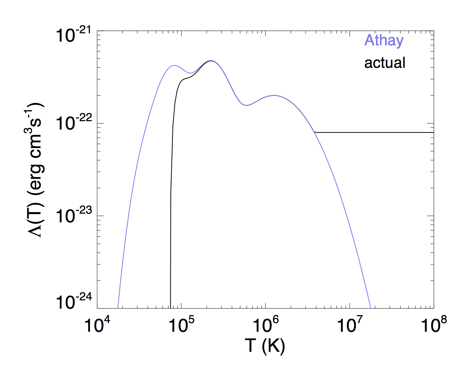
Figure 1: The radiative loss function as given in Athay (1986) (blue curve), and the modified actual function used, where the radiative loss is suppressed for $T\leq 7\times 10^{4}$ K and is set to constant for $T$ above $3.8\times 10^{6}$ K.

We suppress cooling for $T\leq 7\times 10^{4}$ K so that the smallest pressure scale height of the coolest plasma that can form does not go below two grid points given our simulation resolution. We set the cooling to constant for $T>3.8\times 10^{6}$ K so it follows more closely to the radiative loss given by CHIANTI 7 with coronal abundances (Landi et al., 2012) in the high temperature range near $10^{7}$ K. We use a simple form of empirical coronal heating function that only varies with height following an exponential decay:

$$H=\frac{F}{L_{H}}\frac{R^{2}_{\odot}}{r^{2}}\exp\left[-(r-R_{\odot})/L_{H}\right].$$ (14)

where the input energy flux density is $F=9.74\times 10^{5}\,{\rm ergs}\,{\rm cm}^{-2}{\rm s}^{-1}$, the decay length is $L_{H}=1.948\times 10^{10}$ cm.

The above MHD equations are solved using the “Magnetic Flux Eruption” (MFE) code that has been used in several past simulations of coronal mass ejections (e.g. Fan, 2012, 2016). The code uses a staggered $r$-$\theta$-$\phi$ grid with a second-order accurate spatial discretization. A second-order TVD Lax-Friedrichs scheme with a reduced numerical diffusive flux (eq. A(3) in Rempel et al., 2009) is used for evaluating the advection terms in the continuity, momentum, and the internal energy equations. For the induction equation, a method of characteristics that is upwind for the shear Alfvén waves is applied for evaluating the electromotive force (emf) ${\bf v}\times{\bf B}$ and the constrained transport scheme is used to ensure $\nabla\cdot{\bf B}=0$ (Stone & Norman, 1992). No explicit viscosity and magnetic diffusion are included in the momentum and the induction equations. However, numerical diffusions are present as a result of the upwinded evaluations of the fluxes in the momentum equation and the electric field in the induction equation. In the numerical code, the dissipation of kinetic and magnetic energies due to these numerical diffusive fluxes are being evaluated and added to the internal energy as non-adiabatic heating, in addition to the explicit empirical coronal heating term $H$ in the above internal energy equation. To evaluate the numerical dissipation of magnetic energy, we take the difference between the actual (upwinded) evaluation of the emf $({\bf v}\times{\bf B})_{\rm actual}$ and a direct linear interpolation evaluation of the emf $({\bf v}\times{\bf B})_{\rm int}$ at the cell edges (where the emf is defined on the staggered grid). From this difference emf ${\bf E}_{\rm num}=({\bf v}\times{\bf B})_{\rm actual}-({\bf v}\times{\bf B})_{\rm int}$ we evaluate the conversion of magnetic energy into thermal energy due to numerical diffusion as $-(1/4\pi){\bf E}_{\rm num}\cdot(\nabla\times{\bf B})$, which is added to the right hand side of the internal energy equation. Here $\nabla\times{\bf B}$ is computed with a simple centered finite difference. Similarly, in the evaluation of the advection term $\nabla\cdot(\rho{\bf v}{\bf v})$ of the momentum equation, the actual upwinded evaluation of the momentum flux $(\rho{\bf v}{\bf v})_{\rm actual}$ can be written as $(\rho{\bf v}{\bf v})_{\rm int}+{\cal D}_{\rm num}$ where $(\rho{\bf v}{\bf v})_{\rm int}$ is a direct linear interpolation evaluation of the momentum flux and ${\cal D}_{\rm num}$ denotes the additional numerical diffusive flux due to the upwinding in the modified TVD Lax-Friedrichs scheme. Then we evaluate $({\cal D}_{\rm num}\cdot\nabla)\cdot{\bf v}$ as the numerical viscous dissipation added to the right hand side of the internal energy equation, where the derivatives for the $\nabla$ in the above expression is evaluated using simple centered finite differences. The (numerical) energy dissipation is the strongest at current sheets and shocks and is being put back into the internal energy as heating.

The code uses an explicit 3rd order Runge-Kutta scheme for temporal discretization. Under typical coronal conditions, the CFL time step required for the parabolic (field-aligned) heat conduction is often orders of magnitude smaller than the time step required for the hyperbolic advection terms. Here we have used the hyperbolic heat conduction approach described in section 2.2 in Rempel (2017) to circumvent the stringent timestep constraint. Instead of using equation 10, we solve the following equation for the heat flux ${\bf q}_{s}$:

$$\tau_{s}\frac{\partial{\bf q}_{s}}{\partial t}=\left(-\kappa_{0}T^{5/2}\hat{\bf b}\hat{\bf b}\cdot\nabla T-{\bf q}_{s}\right),$$ (15)

where $\tau_{s}$ represents a finite time scale for ${\bf q}_{s}$ to evolve towards the Spitzer heat flux, and it is set to

$$\tau_{s}=\frac{\kappa_{0}T^{7/2}}{e}\frac{(\Delta t)^{2}}{(f_{\rm cfl}\Delta x_{\rm min})^{2}},$$ (16)

where $\Delta t$ denotes the dynamic CFL time step determined from all of the other advection terms, $f_{\rm cfl}$ is the CFL number used, and $\Delta x_{\rm min}$ is the smallest grid size. With the addition of equation 15, we have 3 more dependent variables (3 vector component of ${\bf q}_{s}$) which we advance using the same Runge-Kutta scheme with the right hand side of equation 15 evaluated with a simple 2nd order finite difference scheme on the staggered grid (without the need for upwinded interpolation). As described in Rempel (2017), the introduction of ${\bf q}_{s}$ given by equation 15 produces a wave-like equation for $T$ (or internal energy $e$), and the above specification of $\tau_{s}$ by equation 16 ensures that the effective wave speed does not require a CFL time step that is below $\Delta t$. Rempel (2017) showed that the hyperbolic heat conduction approach gives a good approximation of the evolution produced by the parabolic heat conduction if the required $\tau_{s}$ is small compared to the thermal diffusion time scale of interest. For our current simulations, we have tested this hyperbolic heat conduction approach by comparing the results obtained using this approach to those produced by solving for the parabolic heat conduction term using operator split and sub-cycling with the explicit Super TimeStepping scheme of Meyer et al. (2012), and we found good agreement in the resulting evolution.

Our simulations are carried out in a spherical wedge domain with $r\in[R_{\odot},11.47R_{\odot}]$, $\theta\in[75^{\circ},105^{\circ}]$, and $\phi\in[-\phi_{\rm max},\phi_{\rm max}]$, where we have run cases with $\phi_{\rm max}=75^{\circ}$ and $\phi_{\rm max}=37.5^{\circ}$, to accommodate flux ropes with different lengths and total twists. We use a grid of $504(r)\times 196(\theta)\times 960(\phi)$ for the longer domain with $\phi_{\rm max}=75^{\circ}$ and a grid of $504(r)\times 196(\theta)\times 480(\phi)$ for the domain with $\phi_{\rm max}=37.5^{\circ}$. The grid is uniform in $\theta$ and $\phi$ and stretched in the $r$ direction, with a grid size of $dr=0.002727R_{\odot}=1.898$ Mm for $r<1.79R_{\odot}$ and it increases geometrically to about $0.19R_{\odot}$ at the outer boundary of $r=11.47R_{\odot}$.

For the thermodynamic conditions at the lower boundary of the simulation domain, we assume a fixed transition region temperature of $5\times 10^{5}$ K, and adjust the base pressure $p_{R_{\odot}}$ in the following way:

$$\frac{\partial p_{R_{\odot}}}{\partial t}=\frac{1}{\tau}\left(p_{\rm reb}-p_{R_{\odot}}\right)$$ (17)

where,

$$p_{\rm reb}=C\left(\kappa_{0}T^{5/2}\frac{dT}{dr}\right)_{r={R_{\odot}}}$$ (18)

such that the base pressure is driven towards a value $p_{\rm reb}$ that is proportional to the downward heat conduction flux, in a time scale of $\tau$, to crudely represent the effect of chromospheric evaporation. The expression (eq. [18]) for the coronal base pressure $p_{\rm reb}$ is given by the radiative energy balance (reb) model of Withbroe (1988). Here we have used $C=1.32\times 10^{-6}$ in CGS units and $\tau=357$ sec. We have chosen $\tau$ to be on the order of the sound crossing time of the chromosphere. Thus the (time-varying) pressure $p_{R_{\odot}}$ prescribed at the bottom boundary via equation 17 provides a mass reservoir for the corona plasma and the solar wind that is heated and accelerated in the domain. Note also this mass reservoir at the lower boundary is fixed at the temperature of $5\times 10^{5}$ K, so any cool prominence condensation that develops in the corona is not directly carried into the domain from the lower boundary, but forms after emerging into the coronal domain.

At the lower boundary we also impose a kinematic magnetic flux transport by specifying a time-dependent transverse electric field ${\bf E}_{\perp}|_{r=R_{\odot}}$. Setting the electric field to zero would correspond to a rigid anchoring or line-tying lower boundary. At certain time periods during the simulations, we impose the emergence of a twisted magnetic torus at the lower boundary by specifying the electric field:

$${\bf E}_{\perp}|_{r=R_{\odot}}={\hat{\bf r}}\times\left[\left(-\frac{1}{c}\,{\bf v}_{0}\times{\bf B}_{\rm torus}(R_{\odot},\theta,\phi,t)\right)\times{\hat{\bf r}}\right].$$ (19)

that corresponds to the upward advection at a constant velocity ${\bf v}_{0}$ of a magnetic field structure ${\bf B}_{\rm torus}$ given below, defined in its own local spherical polar coordinate system ($r^{\prime}$, $\theta^{\prime}$, $\phi^{\prime}$) whose origin is located at ${\bf r}={\bf r}_{0}=(r_{0},\theta_{0},\phi_{0})$ of the sun’s spherical coordinate system and whose polar axis is parallel to the polar axis of the sun’s spherical coordinate system:

$${\bf B}_{\rm torus}=\nabla\times\left(\frac{A(r^{\prime},\theta^{\prime})}{r^{\prime}\sin\theta^{\prime}}\hat{\bf\phi^{\prime}}\right)+B_{\phi^{\prime}}(r^{\prime},\theta^{\prime})\hat{\bf\phi^{\prime}},$$ (20)

where

$$A(r^{\prime},\theta^{\prime})=\frac{1}{2}qa^{2}B_{t}\exp\left(-\frac{\varpi^{2}(r^{\prime},\theta^{\prime})}{a^{2}}\right),$$ (21)

$$B_{\phi^{\prime}}(r^{\prime},\theta^{\prime})=\frac{aB_{t}}{r^{\prime}\sin\theta^{\prime}}\exp\left(-\frac{\varpi^{2}(r^{\prime},\theta^{\prime})}{a^{2}}\right),$$ (22)

where $a$ is the minor radius of the torus, $\varpi=(r^{\prime 2}+R^{\prime 2}-2r^{\prime}R^{\prime}\sin\theta^{\prime})^{1/2}$ is the distance to the circular axis of the torus, in which $R^{\prime}$ is the major radius of the torus, $q/a$ denotes the rate of field line twist (rotation in rad per unit length) about the circular axis of the torus, and $B_{t}a/R^{\prime}$ gives the field strength at the circular axis of the torus. For all the simulations in this work, we have $a=0.04314R_{\odot}$ and $q/a=-0.0166$ rad ${\rm Mm}^{-1}$. We have used different values for the major radius $R^{\prime}$ and axial field strength $B_{t}a/R^{\prime}$, to carry out simulations with different lengths and hence different total twist of the emerged portion of the flux rope (since here we fix the twist rate $q/a$ of the torus). The different cases of $R^{\prime}$ used will be given later in section 3.1. Also for specifying the flux emergence via ${\bf E}_{\perp}|_{r=R_{\odot}}$ given by (19), it is assumed that the torus’ center position ${\bf r}_{0}$ is initially located at $(r_{0}=R_{\odot}-a-R^{\prime},\,\theta_{0}=\pi/2,\,\phi_{0}=0)$ (thus the torus is initially entirely below the surface) and moves bodily towards the lower boundary at a constant velocity ${\bf v}_{0}=v_{0}\hat{{\bf r}}_{0}$, with $v_{0}=1.95$ km/s, until a time when the emergence is stopped and ${\bf E}_{\perp}|_{r=R_{\odot}}$ is set to zero. The velocity field at lower boundary is specified to be uniformly $v_{0}\hat{{\bf r}}_{0}$ in the area where the emerging torus intersects the lower boundary and zero everywhere else. Note that $\hat{{\bf r}}_{0}$ denotes a constant unit vector that does not change with position (unlike $\hat{\bf r}$) - it is the direction of the position vector ${\bf r}_{0}$ of the center of the torus. The imposed advection speed $v_{0}$ is orders of magnitude smaller than the Alfvén and the sound speed in the coronal domain to ensure that the emerging flux rope is allowed to evolve quasi-statically during the driving flux emergence phase. For the side boundaries of the simulation domain, we assume non-penetrating stress-free boundary for the velocity field and perfectly electric conducting walls for the magnetic field. For the top boundary, we use a simple outward extrapolating boundary condition that allows plasma and magnetic field to flow through.

Here we comment on the use of the semi-relativistic MHD. The last term on the right hand side of equation 2 represents the semi-relativistic correction to the classical MHD momentum equation when the Alfvén speed $v_{a}$ becomes relativistic (becomes comparable to the speed of light $c$) while the bulk plasma speed and the sound speed remain non-relativistic (e.g. Gombosi et al., 2002; Rempel, 2017). This is also known as the “Boris correction”. It effectively increases the inertia for acceleration perpendicular to the magnetic field and limits the Lorentz force. In regions of the solar corona with strong magnetic field, the Alfvén speed can become extremely high (approaching or even exceeding speed of light), and therefore the semi-relativistic correction is appropriate. Furthermore, the extreme Alfvén speed can impose stringent numerical time stepping constraint for classical MHD. Thus by using the semi-relativistic correction and also artificially reducing the speed of light $c$, one can take significantly larger time steps for numerical integration (e.g. Gombosi et al., 2002; Rempel, 2017). This is particularly useful and appropriate for the long quasi-static evolution phase where the coronal flux rope is built-up under the streamer as a result of flux emergence and/or tether-cutting reconnection. In our simulations of this work, we have set $c=1951$ km/s, which is always above the the peak Alfvén speed in the apex cross-section of the emerged flux rope, but below the peak Alfvén speed for the entire domain, which is found either in the open-field solar wind outflow region in the lower corona or at the lower boundary, reaching about $3000$ km/s. In this way we are able to take larger time steps (than that with classic MHD) through the long quasi-static evolution phase, but still properly model the acceleration of the flux rope during the dynamic eruption phase. There are two major effects of using an artificially reduced speed of light $c$. One is that it increases the inertia for acceleration perpendicular to the direction of the magnetic field and thus can alter the acceleration of the flux rope during the onset of eruption. The other is that it also reduces the effective numerical viscosity and diffusivity by reducing the maximum speed used for the upwinded evaluation of the advection fluxes (Rempel, 2017), and hence can reduce the numerical diffusion during the long quasi-static phase of the evolution. Therefore in regard to the second effect, the simulation without the Boris correction and the reduced speed of light may not be “more accurate” or considered a “reference” solution. Through test simulations with varying $c$, we find that if we reduce $c$ too much, to below about 1/2 of the Alfvén speed of the flux rope apex cross section, we begin to see significant decrease of the peak acceleration of the flux rope during the onset of the eruption. We find that if we use $c$ comparable to or greater than the peak Alfvén speed in the apex cross-section of the flux rope (as is the case here with $c=1951$ km/s), the dynamic evolution of the eruption remains very close to that obtained without the Boris correction.

3 Results

3.1 The initial helmet streamer fields

For the initial state of the simulations, we initialize two different 2D quasi-steady solutions of a coronal streamer with a background solar wind. We initialize a wide streamer (WS) solution and a narrow streamer (NS) solution, for which the normal magnetic flux distributions at the lower boundary are bipolar bands with $B_{r}(R_{\odot},\theta,\phi)=B_{s}(\theta)$, where $B_{s}(\theta)$ used for the WS and NS solutions are shown in Figure 2(a) and Figure 2(b) respectively.

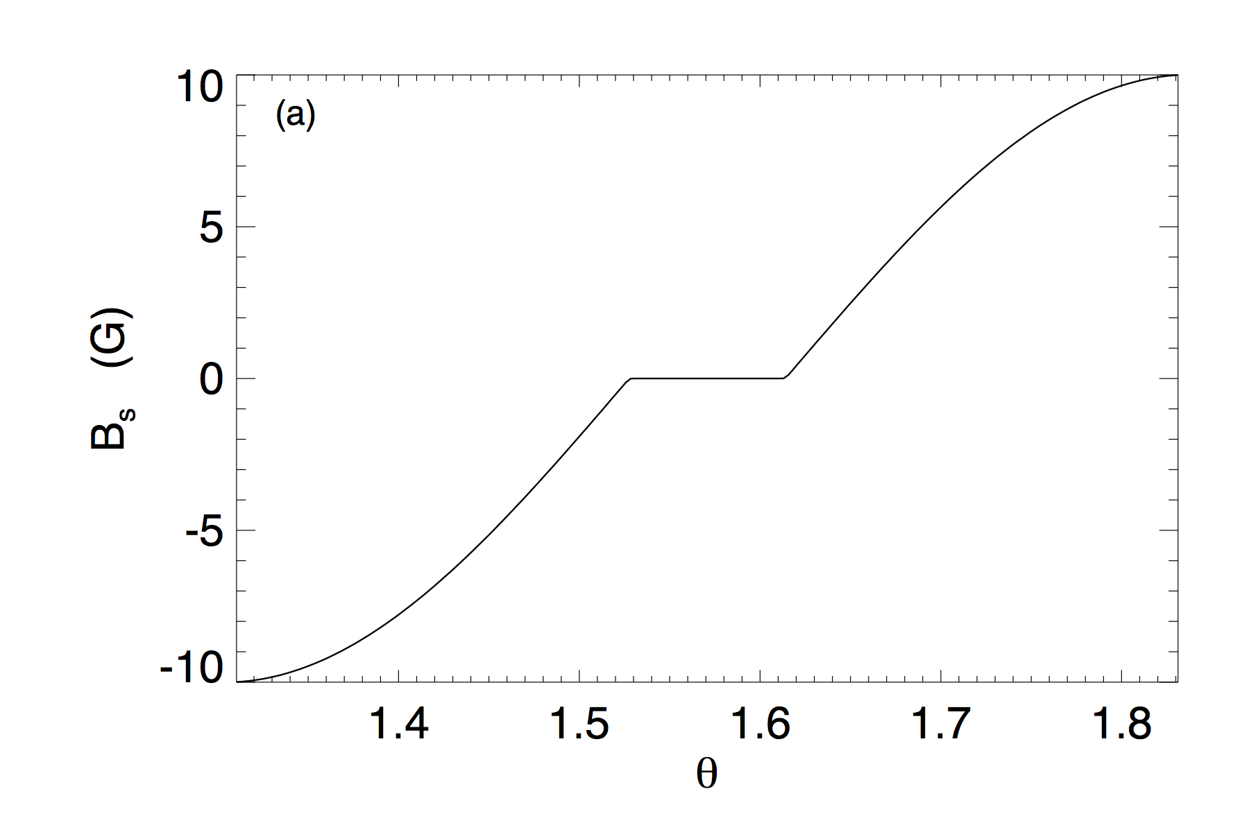
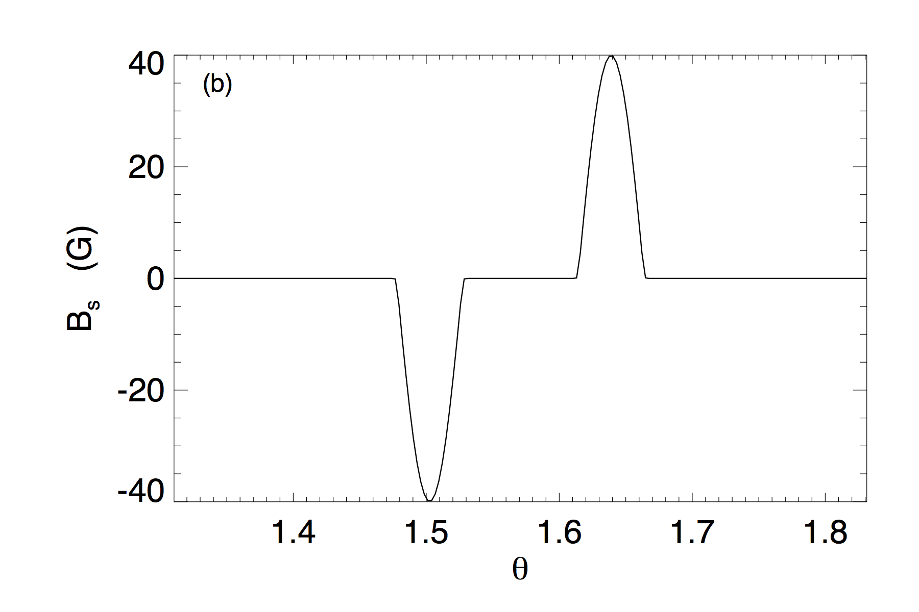
Figure 2: The lower boundary normal magnetic field $B_{s}(\theta)$ used for the WS (panel a) and NS (panel b) initial streamer solutions

With the lower boundary normal magnetic field distribution given above, we first construct an initial potential magnetic field together with a hydrostatic atmosphere with a specified temperature profile that increases linearly from $5\times 10^{5}$ K at the lower boundary to $1.5\times 10^{6}$ K at $22.5$ Mm height, and then remains constant to the outer boundary at about $11.5R_{\odot}$. The initial potential field is a 2D arcade field (invariant in $\phi$) given by ${\bf B}_{p}(r,\theta)=\nabla\Phi(r,\theta)$, where the potential $\Phi$ satisfies the Laplace equation $\nabla^{2}\Phi(r,\theta)=0$. Discretizing the 2D Laplace equation for $\Phi$ with the appropriate boundary conditions lead to a block tridiagonal system, which is solved using the routine blktri.f in the FISHPACK math library of the National Center for Atmosphereic Research (NCAR) based on the generalized cyclic reduction scheme developed by P. Swatztrauber of NCAR. We then lower the pressure at the outer boundary of the initial static state to initiate an outflow, and let the system relax with time (following the MHD equations) until a quasi-steady state is reached and the potential field is stretched out into a streamer configuration. The relaxed WS initial streamer solution is shown in Figure 3,

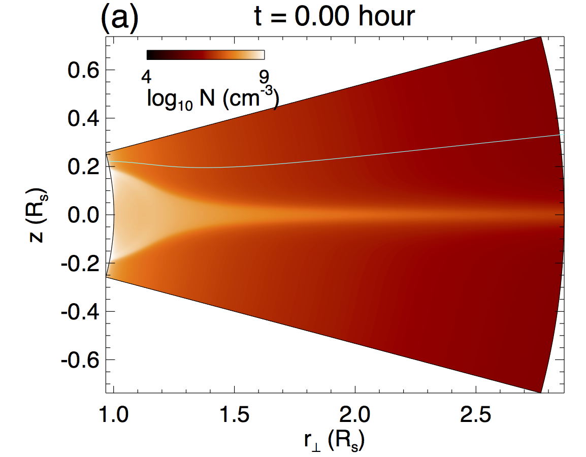
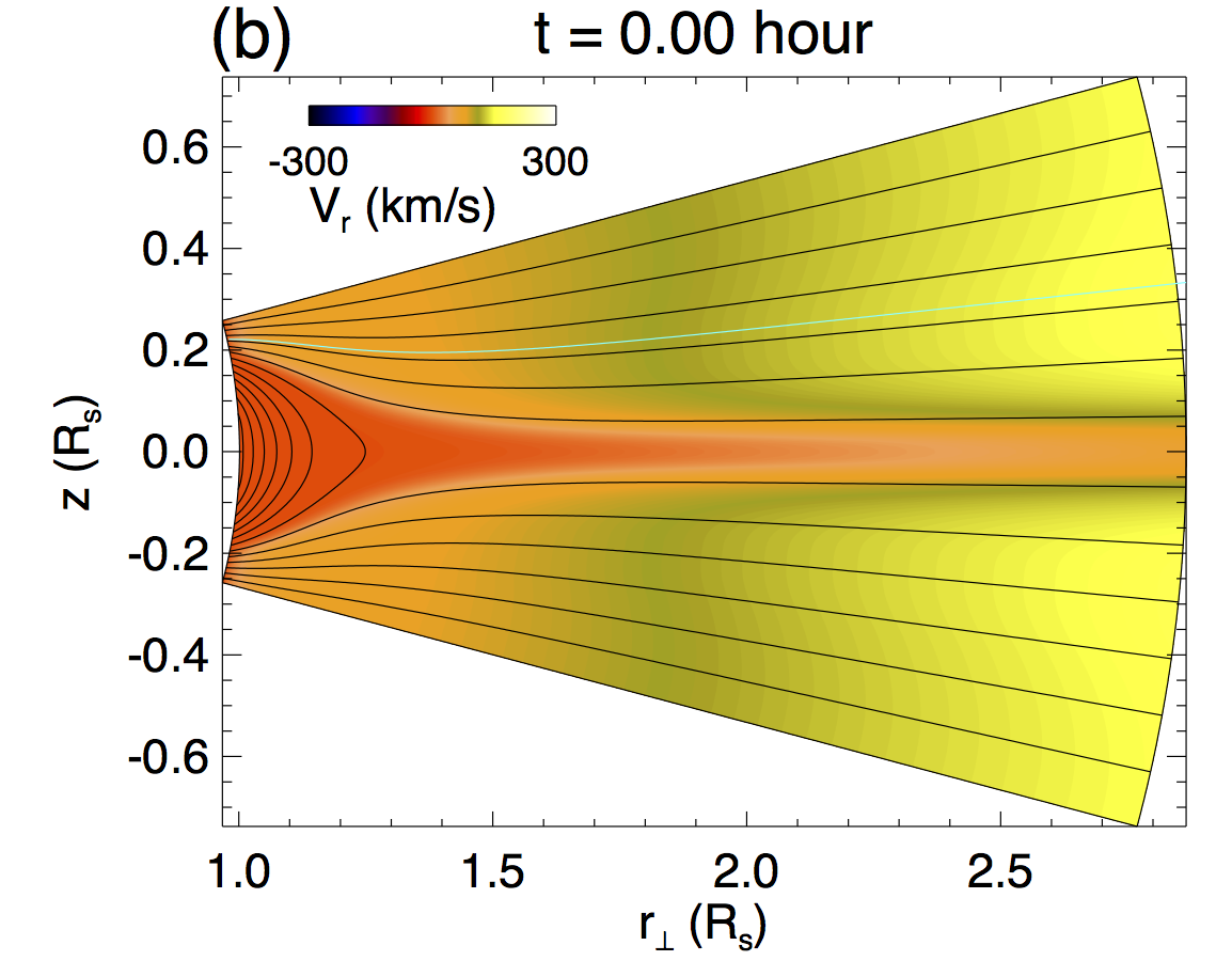
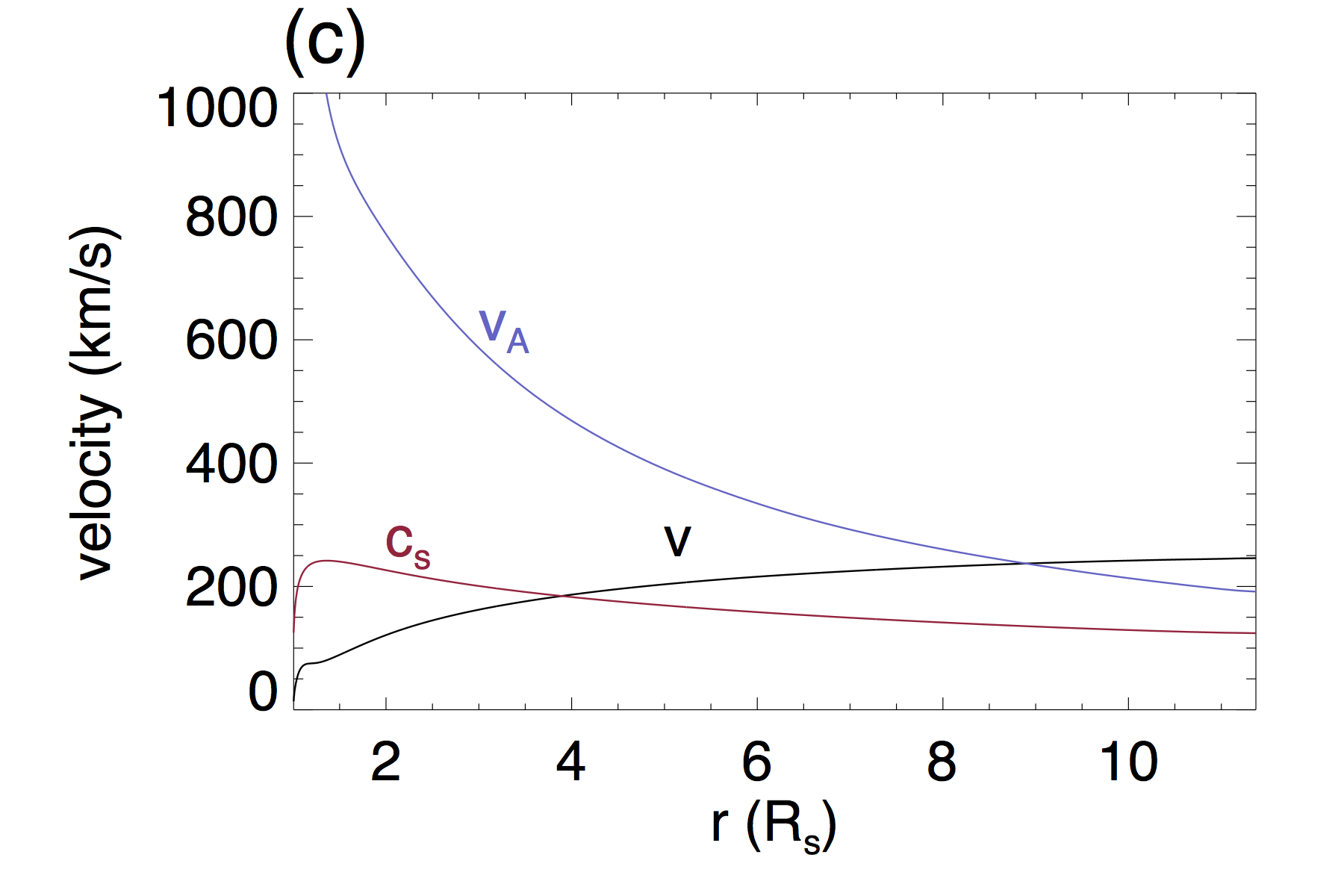
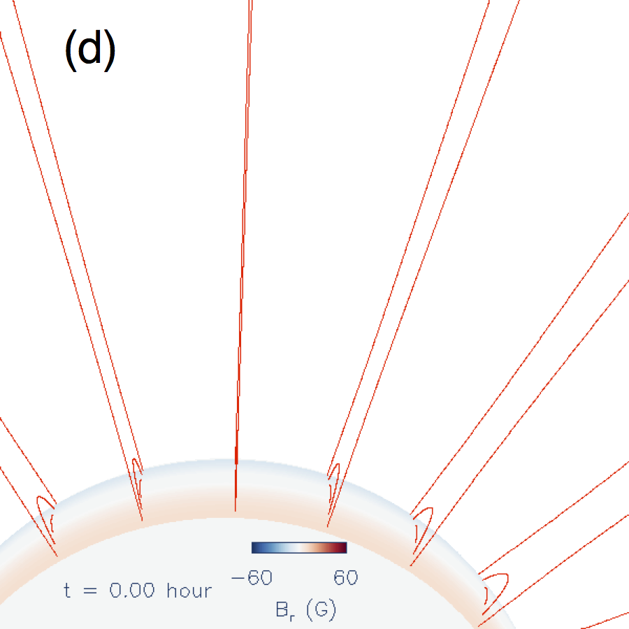
Figure 3: The WS initial state: (a) shows the density in the meridional cross-section; (b) shows the radial velocity in the meridional cross-section over plotted with contours of the magnetic field lines; (c) shows the parallel velocity $V$, the Alfvén speed $V_{a}$, and the sound speed $C_{s}$, along an open field line (the green line shown in panel (a) and (b)); (d) shows a 3D view of the initial field lines in the simulation domain with the lower boundary spherical surface colored based on the normal magnetic field $B_{r}$.

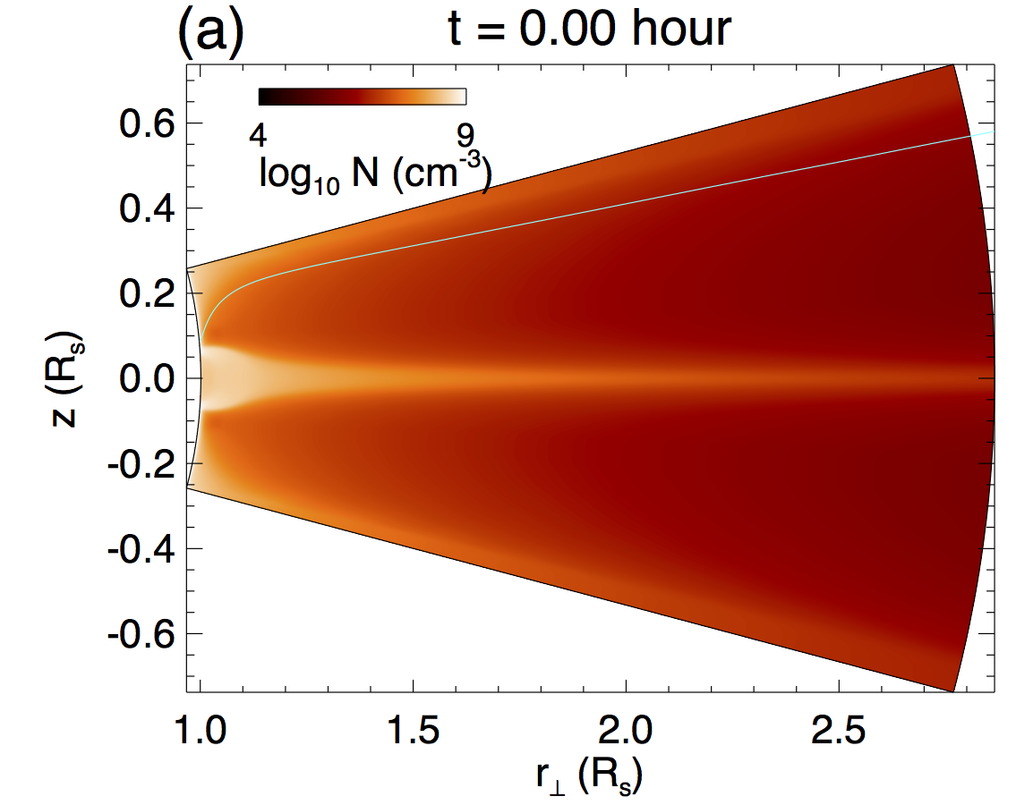
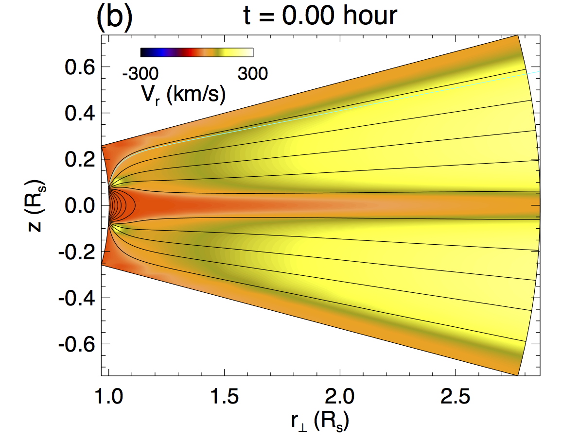
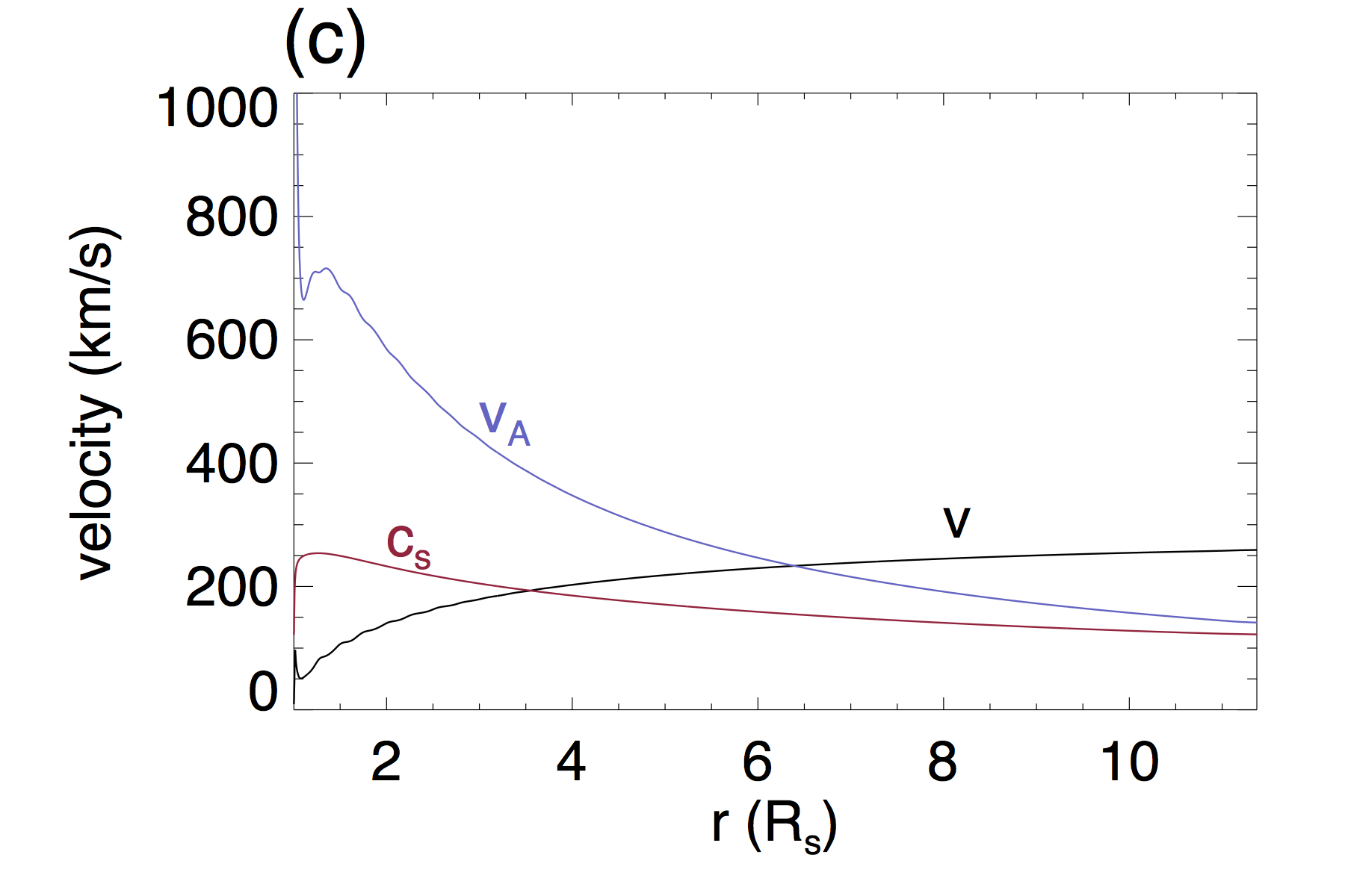
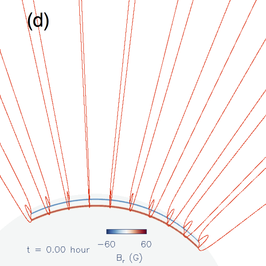
Figure 4: Same as Fig. 3 but for the NS initial state.

where we see a helmet streamer with a denser helmet dome of closed magnetic field in approximately static equilibrium, in an ambient low density open field region with a solar wind outflow. The outflow speed, and the sound speed and the Alfvén speed along an open field line (indicated by the green field line in the top two panels) are shown in the bottom panel of Figure 3. The wind speed becomes super-sonic at about $4R_{\odot}$ and super-Alfvénic at about $9R_{\odot}$, reaching a peak speed of about 250 km/s at the outer boundary at about $11.5R_{\odot}$. The solar wind obtained here is a thermally driven wind heated by the highly simplified empirical coronal heating function given in equation 14. The peak wind speed reached at $11.5R_{\odot}$ is significantly lower than that reached by the fast wind in solar coronal holes because here we have not included the acceleration and heating by the Alfvén wave turbulence (e.g. van der Holst et al., 2014). However, with our simple initial solar wind solution, we obtain the partially open coronal magnetic field configuration of a helmet streamer with a denser helmet dome compared to the open field region, in qualitative agreement with observations. Similarly the NS initial streamer solution is shown in Figure 4, where we obtained a significantly smaller and narrower streamer configuration by using a lower boundary normal flux distribution (Figure 2(b)) of a narrower and thinner pair of bipolar bands. The solar wind speed in the open field region is similar to that for the wider steamer case.

Into the dome of the initial streamer field configuration, we drive the emergence of an arched flux rope with a varying length and (hence) total twist, to study the subsequent evolution of the transition from quasi-equilibrium to eruption of the helmet dome. We vary the length and total twist of the emerged flux rope by changing the curvature radius $R^{\prime}$ of the magnetic torus ${\bf B}_{\rm torus}$ used in specifying the the lower boundary electric field for driving the flux emergence as described in section 2. The three numerical simulations carried out, where we use either the WS and NS solution as the initial state, and impose the emergence of the magnetic torus with the different curvature radius $R^{\prime}$ to obtain an emerged flux rope with different length and total twist, are summarized in Table 1. The label of each run is such that the first 2 letters are either “WS” or “NS” denoting which initial helmet streamer solution is used, and the 3rd letter is “L” (for Long), “M” (for Medium), or “S” (for Short), which correspond to setting the curvature radius $R^{\prime}$ to $0.75R_{\odot}$, $0.5R_{\odot}$, or $0.25R_{\odot}$ respectively. The other varying parameters used for each of the runs, i.e. the axial field strength $B_{t}a/R^{\prime}$ of the emerging torus used for specifying the lower boundary electric field, the domain size $\phi_{\rm max}$ in the azimuthal(longitudinal) direction, and the total field line twist reached in the emerged flux rope when the emergence is stopped, are also listed in Table 1.

Table 1: Summary of simulations

case label	initial streamer	$R^{\prime}$ ($R_{\odot}$)	$B_{t}a/R^{\prime}$ (G)	$\phi_{\rm max}$	emerged twist (winds)
WS-L	wide streamer	0.75	100	$75^{\circ}$	1.83
WS-M	wide streamer	0.5	103	$37.5^{\circ}$	1.1
NS-S	narrow streamer	0.25	90	$37.5^{\circ}$	0.6

3.2 Eruption under a wide and a narrow streamer

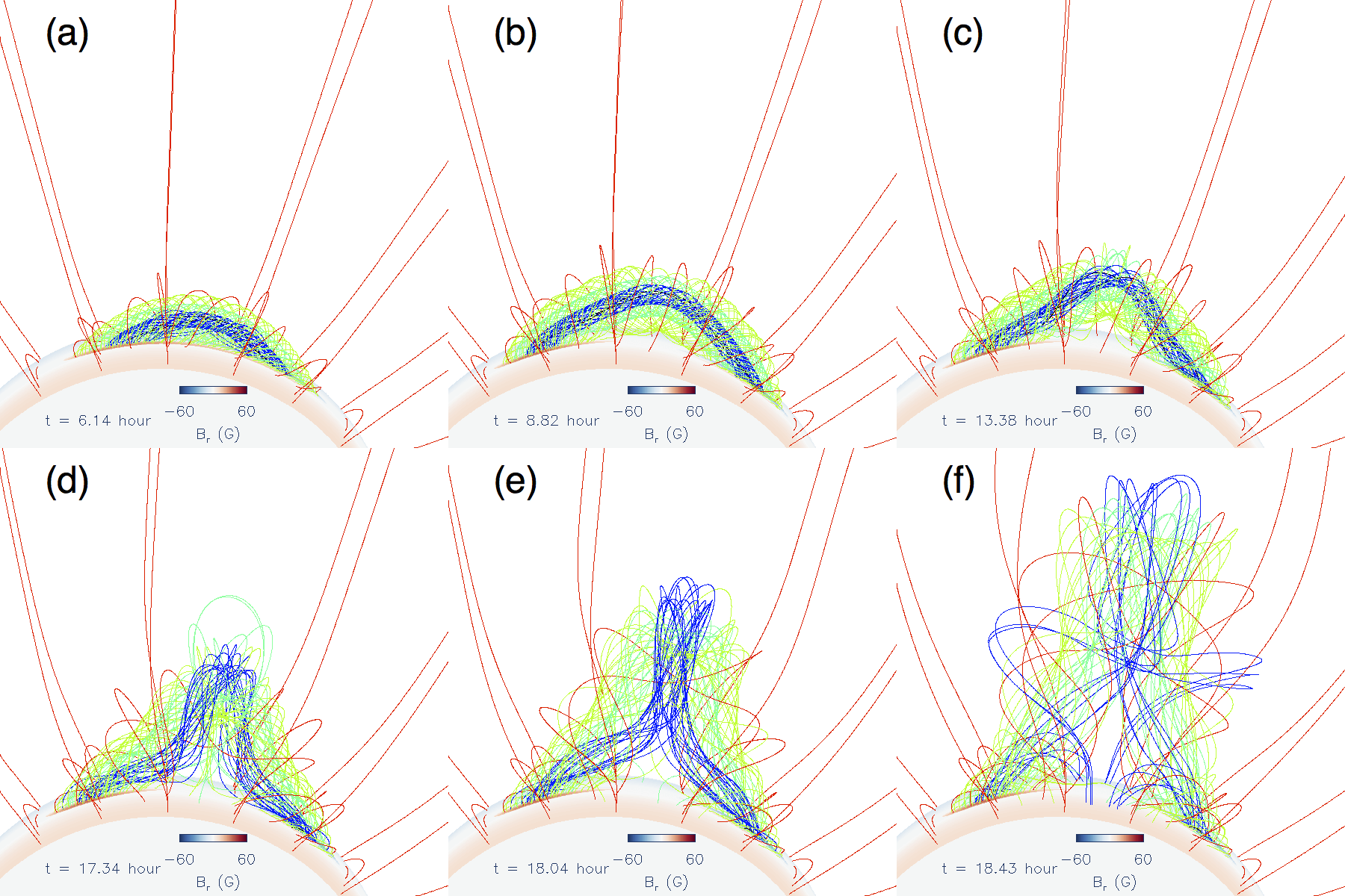
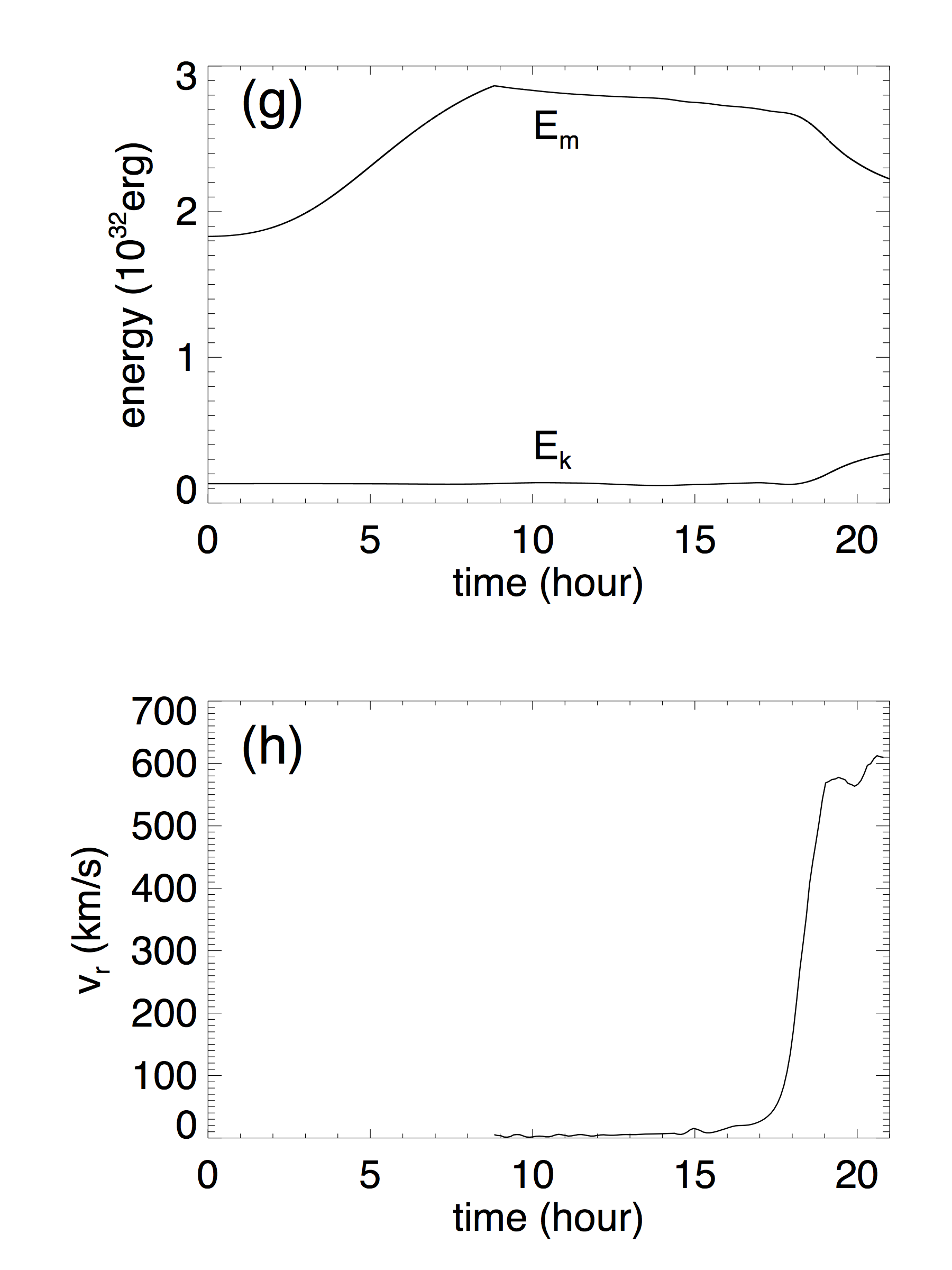
Figure 5: The evolution obtained from simulation case WS-L. Panels (a)-(f) show snapshots of the 3D magnetic field lines. The lower boundary surface is colored with $B_{r}$. The color of the field lines are based on the original flux surfaces as described in the text. Panel (g) shows the evolution of the total magnetic energy $E_{m}$ and total kinetic energy $E_{k}$. Panel (h) shows the evolution of the rise velocity $v_{r}$ tracked at the apex of the emerged flux rope axis. A movie for this figure showing the evolution of the 3D magnetic field, and the evolution of $E_{m}$, $E_{k}$, and $v_{r}$ throughout the course of the simulation (from $t=0$ to about $t=21$ hour) is available in the online version of the paper.

Panels (a)-(f) of Figure 5 show the 3D magnetic field evolution obtained from the simulation case WS-L, where we drive the emergence of a long flux rope at the lower boundary into the wide streamer initial state in an azimuthally long domain. Panels (g) and (h) of Figure 5 show the corresponding evolution of the magnetic energy $E_{m}$, the kinetic energy $E_{k}$, and the rise velocity $v_{r}$ tracked at the apex of the axial field line of the emerged flux rope. A movie corresponding to Figure 5 showing the 3D field evolution and the evolution of $E_{m}$, $E_{k}$, and $v_{r}$, is available in the online version of the paper. The field lines and their colors are selected in the following way. We use a set of fixed foot points in the pre-existing arcade bands outside the emerging flux region and trace the field lines in red. For tracing the field lines (green, blue, and black field lines) from the emerging flux region on the lower boundary, we track a set of foot points that connect to a fixed set of field lines of the subsurface emerging torus and color the field lines based on the flux surfaces of the subsurface torus. The “axial field line” refers to the field line that is traced from the footpoints at the lower boundary that connect to the curved axis of the subsurface emerging torus ${\bf B}_{\rm torus}$. We track the apex position of this field line for evaluating the $v_{r}$ in panel (h) of Figure 5. After the axial field line has reconnected during its coronal evolution, we continue to track the Lagrangian evolution of this apex element by using its velocity, and continue to refer to it as the “apex of the axial field line”. In panel (g) of Figure 5, we see initially (from about $t=0$ hour to $t=8.82$ hour) the magnetic energy increases as the coronal flux rope is built up quasi-statically under the streamer (see also panels (a) and (b) of Figure 5) as a result of flux emergence driven at the lower boundary. The driving flux emergence is stopped at $t=8.82$ hour when the total field line twist about the axial field line of the emerged flux rope reaches 1.83 winds, which is above the critical twist (about $1.25$ winds) for the onset for the kink instability (Hood & Priest, 1981). Subsequently the flux rope becomes kinked due to the development of the helical kink instability (panels (c) and (d) of Figure 5). However the rope remains confined with its apex rising quasi-statically at a low, significantly sub-Alfvén speed and $E_{m}$ decreases slowly, until roughly $t=17.5$ hour (see panels (g) and (h) of Figure 5), when the flux rope’s rise speed begins a significant acceleration, $E_{m}$ begins a rapid decrease and $E_{k}$ begins a significant increase. The period of slow rise phase (from $t=8.82$ hour to roughly $t=17.5$ hour) after the emergence is stopped is found to be significantly longer than the Alfvén transit time $\tau_{A}\approx 0.136$ hour along the flux rope (estimated by computing the Alfvén transit time along the axial field line between the anchored foot points at the time the emergence is stopped), which is a measure of the dynamic time scale. The slow rise phase lasts about 64 $\tau_{A}$. This suggests that the flux rope remains in quasi-equilibrium for the slow rise phase. There is a clear transition at the time of roughly $t=17.5$ hour from the slow rise phase to a dynamic eruption phase, as can be seen in panels (g) and (h) in Figure 5. The flux rope accelerates to a terminal speed of about $600$ km/s, much higher than the ambient solar wind speed, and begins to exit the domain upper boundary at $11.47R_{\odot}$ at about $t=21$ hour.

The 3D coronal magnetic field evolution of another simulation case WS-M is shown in Figure 6, for which we drive the emergence of a shorter, anchored flux rope, and stop the emergence when the total field line twist about the axial field line reaches 1.1 winds between the anchored ends (at $t=8.82$ hour, Figure 6(b)).

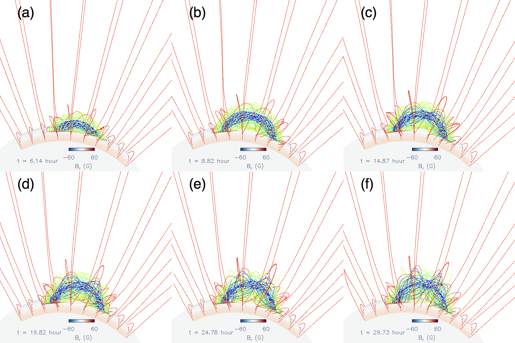
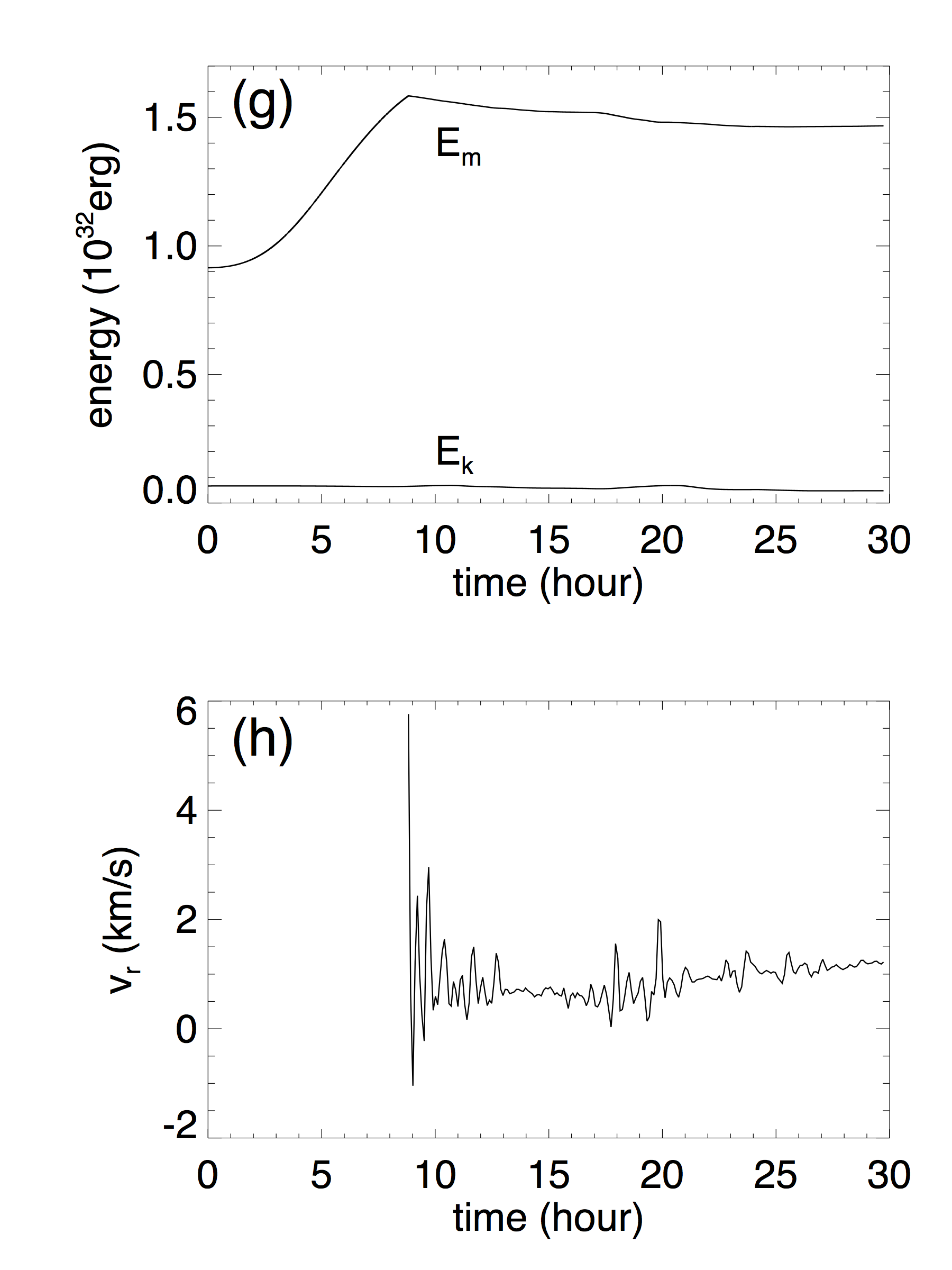
Figure 6: Same as Figure 5 but for the simulation case WS-M.

For this case we see that the flux rope remains stable and well confined in quasi-equilibrium under the streamer for the subsequent evolution of over 20 hours simulated, which corresponds to about $268\tau_{A}$, where $\tau_{A}$ is the Alfvén transit time along the flux rope estimated at the time the emergence is stopped, showing no sign of eruption (see panels (c)-(f) in Figure 6). Panels (g) and (h) of Figure 6 show the evolution of the magnetic energy $E_{m}$, the kinetic energy $E_{k}$, and the rise velocity $v_{r}$ tracked at the apex of the flux rope axial field line. Again we see the build up of the magnetic energy in the flux emergence phase (from $t=0$ to $t=8.82$ hour), when the emergence of the magnetic torus is imposed at the lower boundary. However, subsequently after the emergence is stopped, the rise velocity remains very small, showing some small oscillations (panel (h) of Figure 6). The magnetic energy $E_{m}$ shows a slow decline which becomes steady later, and the total kinetic energy $E_{k}$ remains fairly steady (with the ambient solar wind). All these indicate that the magnetic flux rope in this case is settling into a stable equilibrium under the helmet. The results of the above two simulation cases indicate that the wide-streamer (WS) pre-existing field is very confining, such that the flux rope does not erupt until sufficiently high twist (significantly higher than 1 wind of field line twist) is built up for the kink instability to set in, which brings the apex of the kinked flux rope to a rather high height for it to erupt dynamically.

In contrast, Figure 7 shows the evolution for the simulation case NS-S, where we use the narrow streamer field (NS) as the initial state, and drive the emergence of an even shorter flux rope with the total field line twist about the axial field line reaching only about 0.6 winds between the anchored ends when the emergence is stopped (panel (b) of Figure 7).

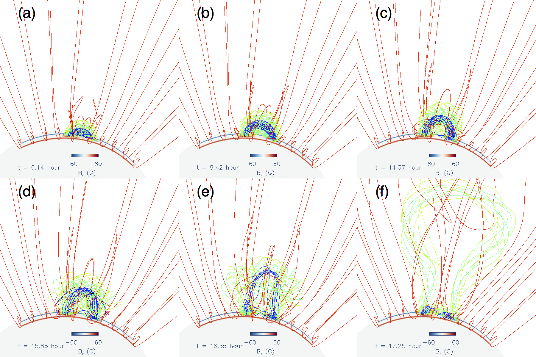
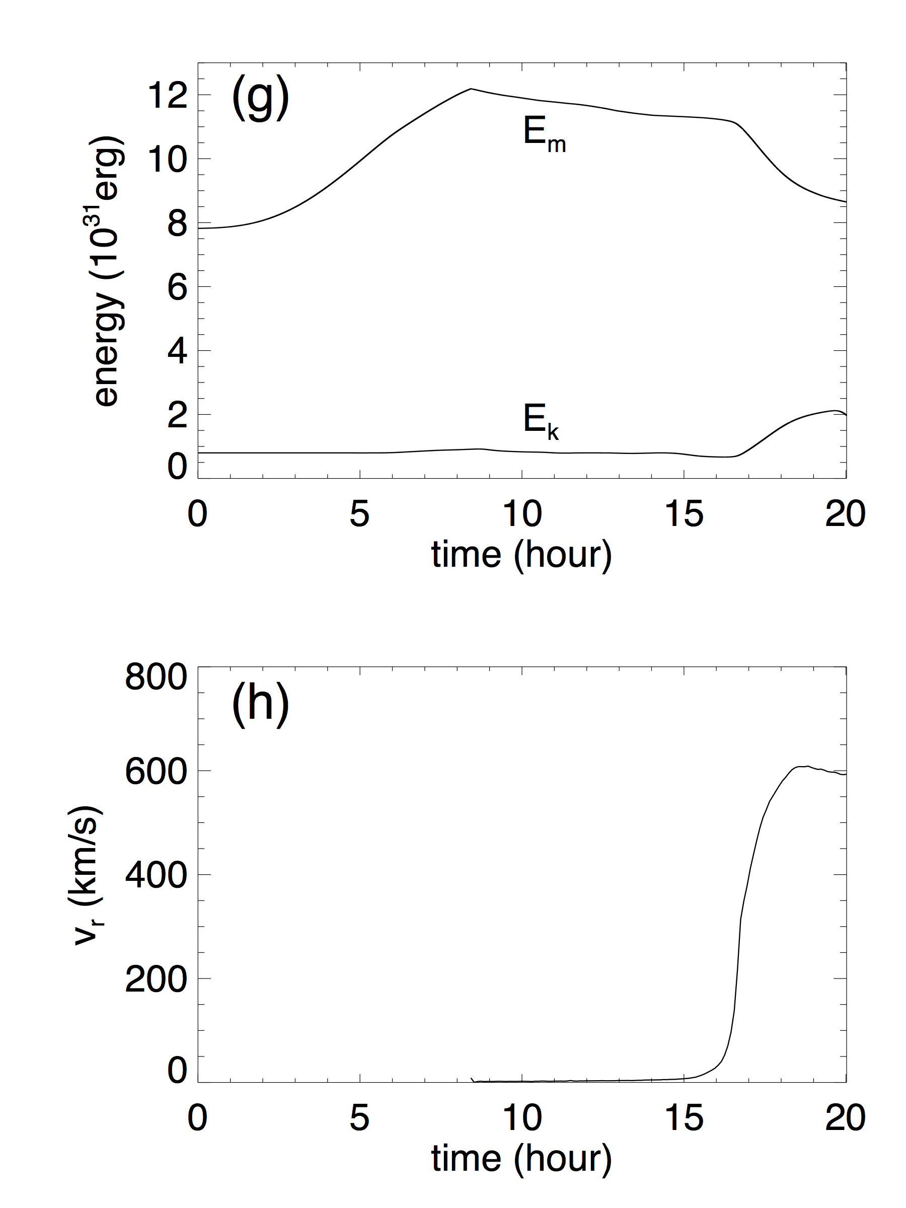
Figure 7: Same as Figure 5 but for the simulation case NS-S. A movie for this Figure is available in the online version of the paper.

Panel (g) and (h) of Figure 7 again show the evolution of the magnetic energy $E_{m}$, the kinetic energy $E_{k}$, and the rise velocity $v_{r}$ tracking the Lagrangian element at the apex of the flux rope axial field line. Even though in this case the twist is well below that for the onset of the kink instability when the emergence is stopped, we see subsequently, similar to the WS-L case, the flux rope undergoes a stage of slow, quasi-static rise with sub-Alfvénic speed for a time span (from about $8.82$ hour to about $16$ hour in panel (h) of Figure 7, also panels (b)-(d) in Figure 7) that is significantly longer than the Alfvén crossing time $\tau_{A}$, about $180\tau_{A}$. At roughly $t=16$ hour, a transition to dynamic eruption occurs with the flux rope undergoes a significant acceleration to a terminal speed of about $600$ km/s and with the total magnetic energy $E_{m}$ showing a significant decrease and the total kinetic energy $E_{k}$ showing a significant increase (see panels (g) and (h) in Figure 7 and panels (d)-(f) of Figure 7). Since the total twist of the flux rope is significantly below the critical limit for the onset of the kink instability, the dynamic eruption in this case is most likely due to the onset of the torus instability when the flux rope rises to a critical height of sufficiently steep decline of the corresponding potential field (e.g. Kliem & Török, 2006; Isenberg & Forbes, 2007). In this case the smaller streamer field is less confining and the flux rope is able to reach the (lower) critical height for the torus instability to set in first.

The quasi-static rise of the flux rope after the emergence is stopped is due to the tether-cutting reconnection in a current sheet that forms underlying the flux rope, similar to what was found in Fan (2010). The reconnection continually add “detached” flux to the flux rope as described in Fan (2010), reducing its anchoring and allowing it to rise quasi-statically to the critical height for the onset of the torus instability. The thermal signature of the tether-cutting reconnection is the formation of a hot channel threading under the flux rope, containing heated twisted flux added to the flux rope, as represented by the hot field lines shown in Figure 8.

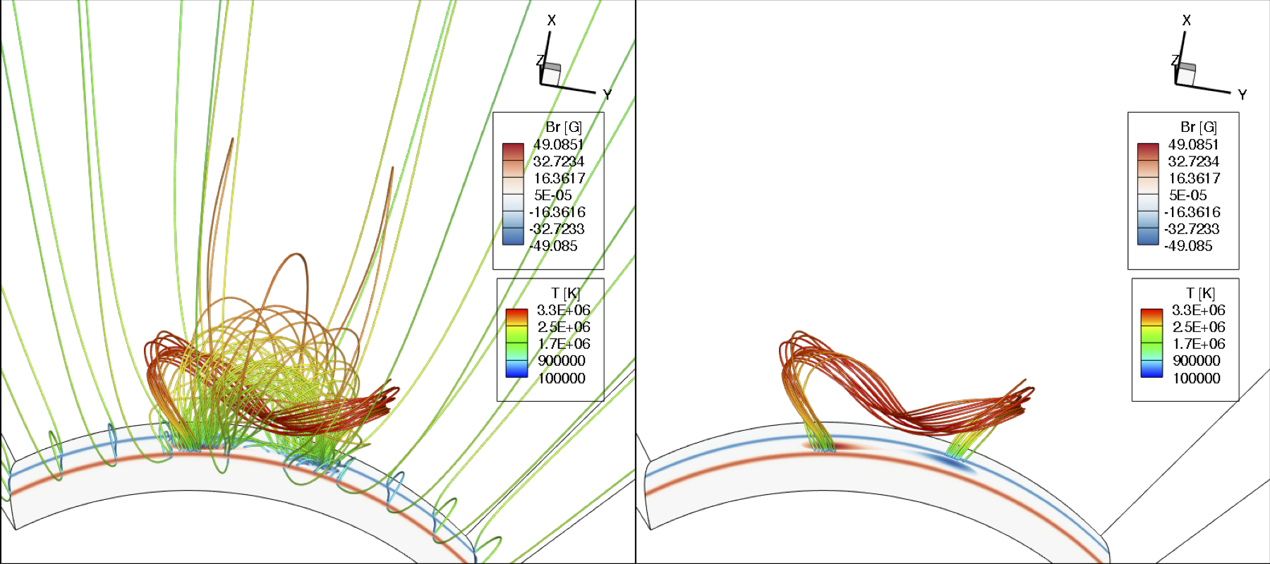
Figure 8: The left panel shows the same field lines as those in Figure 7(c), but colored in temperature and with the addition of the field lines in the hot channel. The right panel shows the hot channel field lines alone. An animation of a rotating view of the field lines is available in the online version.

The left panel of the figure shows the same field lines as those in Figure 7(c), but colored in temperature and with the addition of the field lines in the hot channel, and the right panel shows the hot channel field lines alone. An animation of a rotating view of the field lines in both panels is also available in the online version. Note the hot channel field lines are rooted in the arcade field bands, and therefore represent twisted flux newly added to the flux rope as a result of multiple reconnections of the original arcade field lines with the flux rope field lines. These heated field lines which display a sigmoid shape may correspond to the hot channel observed before and during CMEs by SDO/AIA described in Zhang et al. (2012) and Cheng et al. (2013). The temperature reached by the hot channel in our simulation is about $3.3$ MK, significantly lower than the observed case, which is reported to be as high as $10$ MK. However, this may be due to a much weaker field strength of the flux rope and confining helmet field considered in our simulation. Because of the significantly lower temperature of $3.3$ MK, which is not picked up by the hot peaks of the temperature responses of AIA 131 Å channel (about 11 MK) and AIA 94 Å channel (about 7 MK), and in fact, it is at the local valleys of these two channels’ temperature responses, we do not see the sigmoid brightening corresponding to the hot channel field lines in the modeled emission (not shown here) in these channels.

The top panel of Figure 9 shows the radial acceleration of the tracked Lagrangian element at the apex of the flux rope axial field line as a function of its height, comparing the NS-S case (red curve) and the WS-L case (black curve).

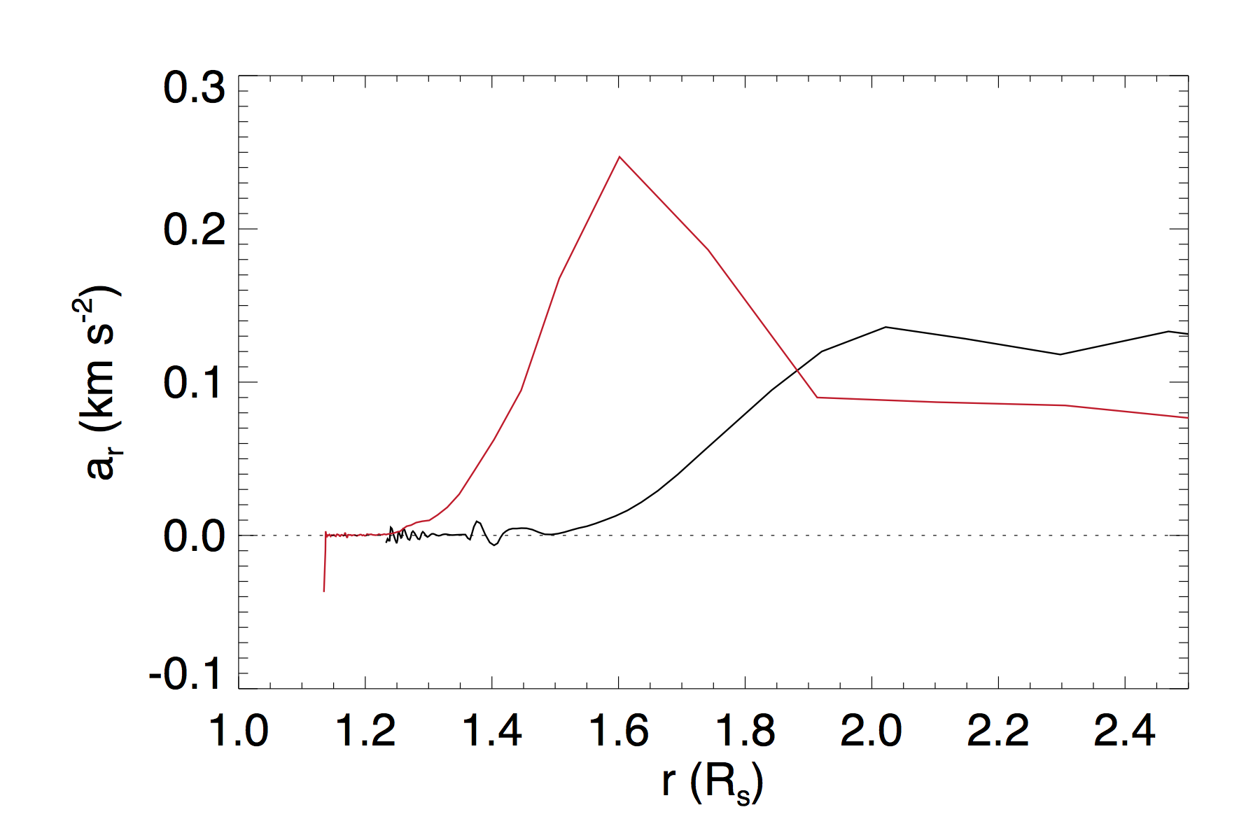
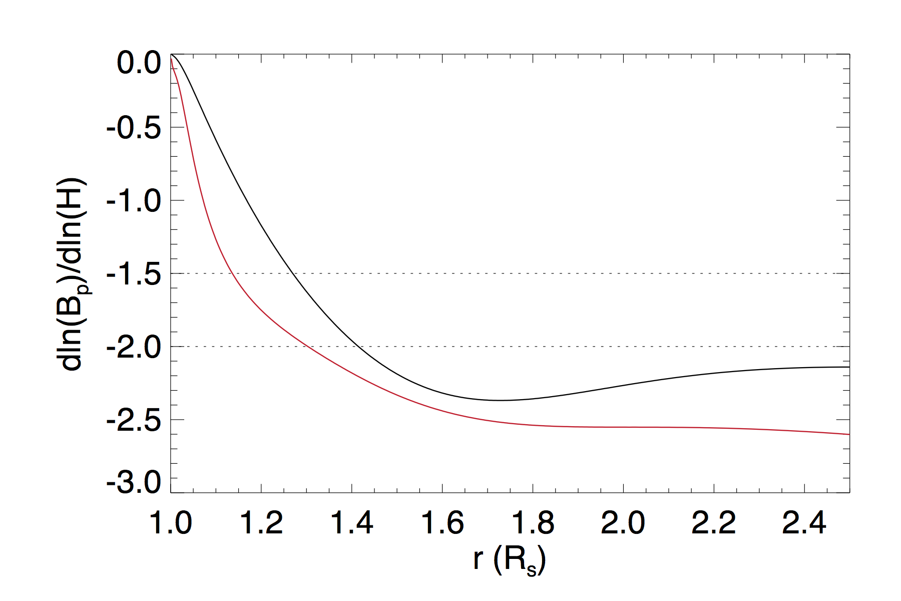
Figure 9: (top panel) Acceleration at the apex of the axial field line as a function of its height position for the WS-L (black curve) and NS-S (red curve) cases, and (bottom panel) the decay rate with height of the corresponding potential field for the WS-L (black curve) and NS-S (red curve) cases when the emergence is stopped (and hence no more change of the lower boundary normal flux distribution and the corresponding potential field).

It can be seen that the monotonic and significant acceleration for the dynamic eruption sets in at a much lower height for the NS-S case compared to the WS-L case. The lower panel of Figure 9 shows the decay rate $dln(B_{p})/dln(H)$ of the corresponding potential field $B_{p}$ with height above the solar surface $H$ along the vertical line through the center of the apex cross-section of the flux rope, for the WS-L (black curve) and NS-S (red curve) cases, when the emergence is stopped (and hence no more change of the lower boundary normal flux distribution and the corresponding potential field afterwards). The decline with height of the potential field for the narrow streamer case NS-S is significantly steeper compared to that for the wide streamer case WS-L, explaining why for the NS-S case the torus instability sets in first at a lower height. From the two panels of Figure 9 we see that for the NS-S case the onset of significant acceleration takes place when the tracked apex of the axial field line reaches about $1.25R_{\odot}$ at which the field decay rate is about -1.9, within the range of critical decline rates (about $-1.$ to $-2.$) for the onset of the torus instability obtained from several theoretical calculations with simplified current loop models (e.g. Titov & Démoulin, 1999; Kliem & Török, 2006; Démoulin & Aulanier, 2010). For the WS-L case on the other hand, the onset of significant acceleration of the flux rope takes place at a much higher height at about $1.55R_{\odot}$ where the field decay rate is about $-2.3$, more than the nominal range of the critical decay rate for the onset of the torus instability. But here the flux rope has already become significantly kinked due to the onset of the kink instability first and its final loss of equilibrium and eruption cannot be simply described by the onset of the torus instability assuming a simple current path. However the need for a sufficiently steep spatial decline of the background potential field in order to achieve an ejective eruption of the flux rope through the onset if the kink instability has also been found in previous MHD simulations of kink unstable flux ropes (e.g. Török & Kliem, 2005).

3.3 Formation and eruption of prominence

The explicit inclusion of the optically thin radiative loss term (eq. 13) in the energy equation provides the driver for the development of radiative (thermal) instability or non-equilibrium (e.g Priest, 2014) which allow the formation of cool dense prominence plasma in the hot rarefied corona. As is described in Priest (2014, section 11.6.3 and references therein) the physical form of the optically thin radiative loss term implies that if a coronal plasma cools locally, the radiative loss increases further leading to a run-away cooling. This is true even if the cooling function $\Lambda$ is constant with $T$ (let alone increasing with decreasing T at certain temperature ranges), because density $N$ would increase with a temperature decrease assuming pressure unchanged at the perturbation. This would further enhance the cooling because of the $N^{2}$ dependence on the radiative loss. The instability can be suppressed by thermal conduction but only if the length scale of the perturbation is not too long. Thus for sufficiently long coronal loops, the radiative instability or non-equilibrium will develop. We find in both the WS-L and WS-M cases, cool prominence condensations with temperature as low as $7.3\times 10^{4}$ K and density as high as $5.6\times 10^{9}{\rm cm}^{-3}$ develop in the corona in the dips of the flux rope field lines. Figure 10 shows the synthetic SDO/AIA 304 Å channel emission, computed by integrating along the line-of-sight (that is the same as that for the view of panels (a)-(f) of Figure 5) through the simulation domain:

$$I_{\rm AIA304}=\int n_{e}^{2}(l)\,f_{\rm AIA304}(T(l))\,dl,$$ (23)

where $l$ denotes the length along the line of sight through the simulation domain, $I_{\rm AIA304}$ denotes the emission intensity at each pixel in units of DN/s/pixel (shown in LOG scale in the images), $n_{e}$ is the electron number density, and $f_{\rm AIA304}(T)$ is the temperature response function that takes into account the atomic physics and the properties of the AIA 304 Å filter. We have obtained the temperature dependent function $f_{\rm AIA304}(T)$ using the SolarSoft routine get_aia_response.pro. The response function $f_{\rm AIA304}(T)$ peaks at the temperature of about $8\times 10^{4}$ K. A movie of the evolution of the synthetic AIA 304 emission is also available in the online version of the paper. We see from Figure 10 and the movie that prominence plasma with temperature around $8\times 10^{4}$ K, forms suspended in the much hotter corona. It lengthens and develops into a suspended loop-like structure during the slow quasi-static rise phase. At the onset of the dynamic eruption of the flux rope, the prominence loop also erupts with its apex rises upward while also showing substantial draining and falling of the prominence plasma at the legs of the prominence loop. Such eruption morphology of a loop like structure with substantial draining at the legs of the loop is often observed in prominence eruptions. Although the flux rope field lines, especially those belonging to the original inner flux surfaces (e.g. the blue field lines in Figure 5), become significantly kinked through the slow rise phase and the onset of the eruption (with a rotation of $\sim 90^{\circ}$), the prominence appears a loop like structure without showing significant kinking when viewed from the same perspective as the flux rope.

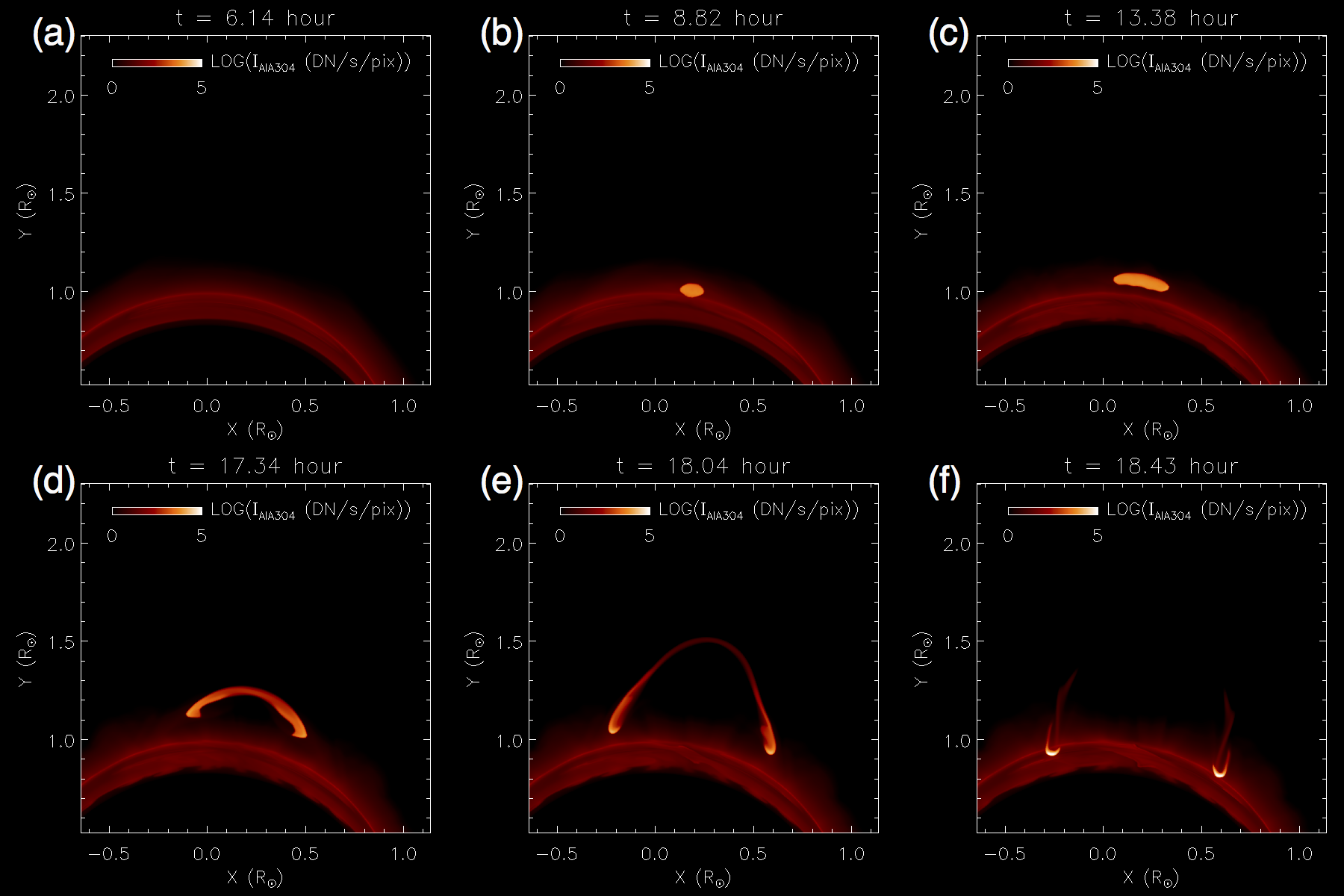
Figure 10: Synthetic SDO/AIA 304 Å channel emission images as viewed from the same line of sight as that of panels (a)-(f) of Figure 5 at the same time instants, computed from the simulation case WS-L. A corresponding movie showing the evolution of the synthetic AIA 304 emission from $t=7.93$ hour to $t=18.4$ hour is also available in the online version.

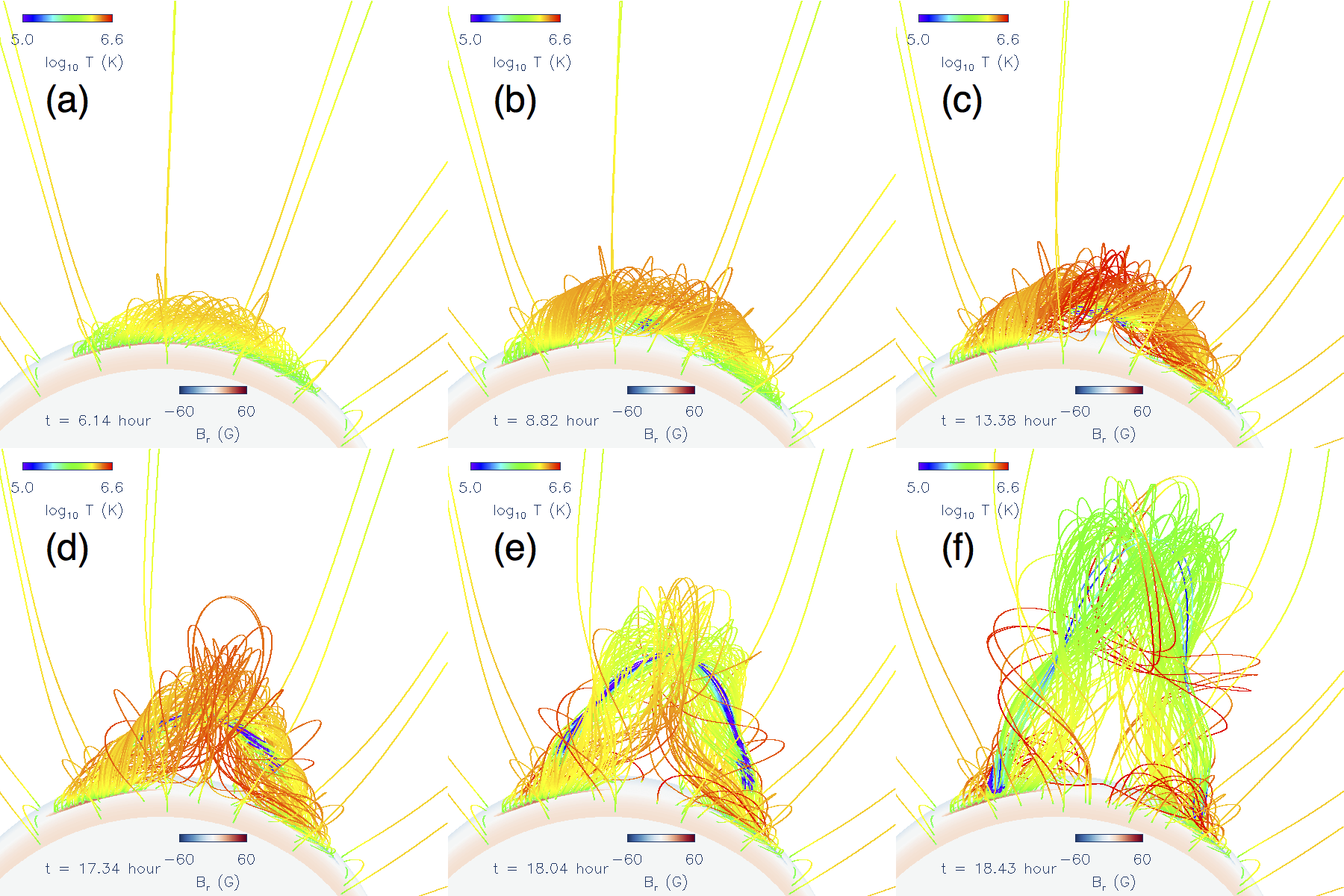
Figure 11: Same as panels (a)-(f) of Figure 5 but with the field lines colored by the temperature, instead of based on the original flux surfaces of the subsurface torus. Also additional prominence carrying field lines are added by tracing field lines from grid points evenly sampled in the region where temperature is below $10^{5}$ K. All images are viewed from the same perspective as the AIA 304 images in Figure 10.

Figure 11 shows the same snapshots of the 3D field lines as those shown in Figure 5 but with the field lines colored by the temperature (instead of based on the original flux surfaces) and also with additional prominence carrying field lines that are traced from grid points sampled in the region where the temperature is below $10^{5}$ K. The dark blue field line segments are where prominence plasma is located, which are somewhat hard to see in panels (b) and (c), as they are still small and partially obscured by other field lines. The location of the prominence condensations is more clearly seen in Figure 12, which show the prominence carrying field lines alone, during the quasi-static rise phase. Comparing to the AIA 304 images at the corresponding time instants in Figure 10, we see that the prominence condensations begin to form in the field line dips in the lower middle part of the flux rope (see panels (b) and (c) of Figure 11 or more clearly panels (a) and (b) of Figure 12). The prominence continues to lengthen during the quasi-static rise phase (panels (c), (d), (e), and (f) in Figure 12) and later erupts into a loop like structure (see the blue field line segments in panels (d), (e) and (f) of Figure 11). Figure 13 shows the top view of the prominence carrying field lines as those in Figure 12 during the quasi-static rise phase. It can be seen that as soon as the prominence condensations develop into an elongated filament (the dark blue segments in panels (b), (c), (d), (e), and (f) in Figure 13), its apparent orientation makes a small angle (about $30^{\circ}$) with the orientation of the magnetic field lines. This is consistent with the magnetic field configuration of solar prominences as inferred from spectropolarimetric observations (e.g. Leroy et al., 1983; Bommier et al., 1994; Orozco Suárez et al., 2014)

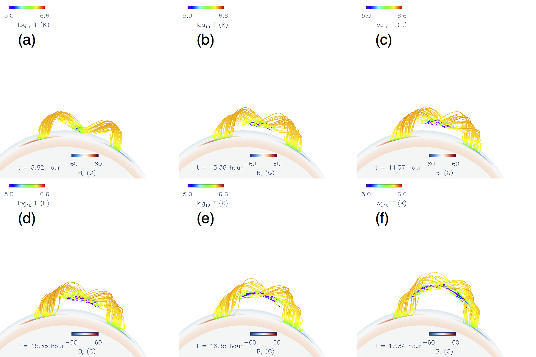
Figure 12: Prominence carrying field lines colored in temperature during the quasi-static rise phase. Field lines are traced from grid points evenly sampled in the region where temperature is below $10^{5}$ K. Note that panels (a), (b), and (f) here correspond to the same time instants and the view as panels (b), (c) and (d) of Figure 11, respectively, but showing only the prominence carrying field lines by themselves.

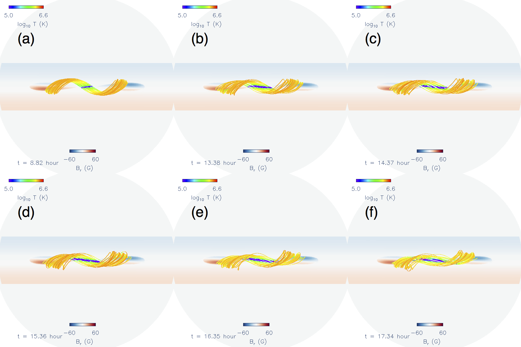
Figure 13: Same as Figure 12, but as viewed from the top

Figure 14 and Figure 15 are snapshots showing the evolution of a tracked prominence field line colored with temperature and density, respectively, along the field line. Movies showing the evolution corresponding to each of these two figures are also available in the online paper.

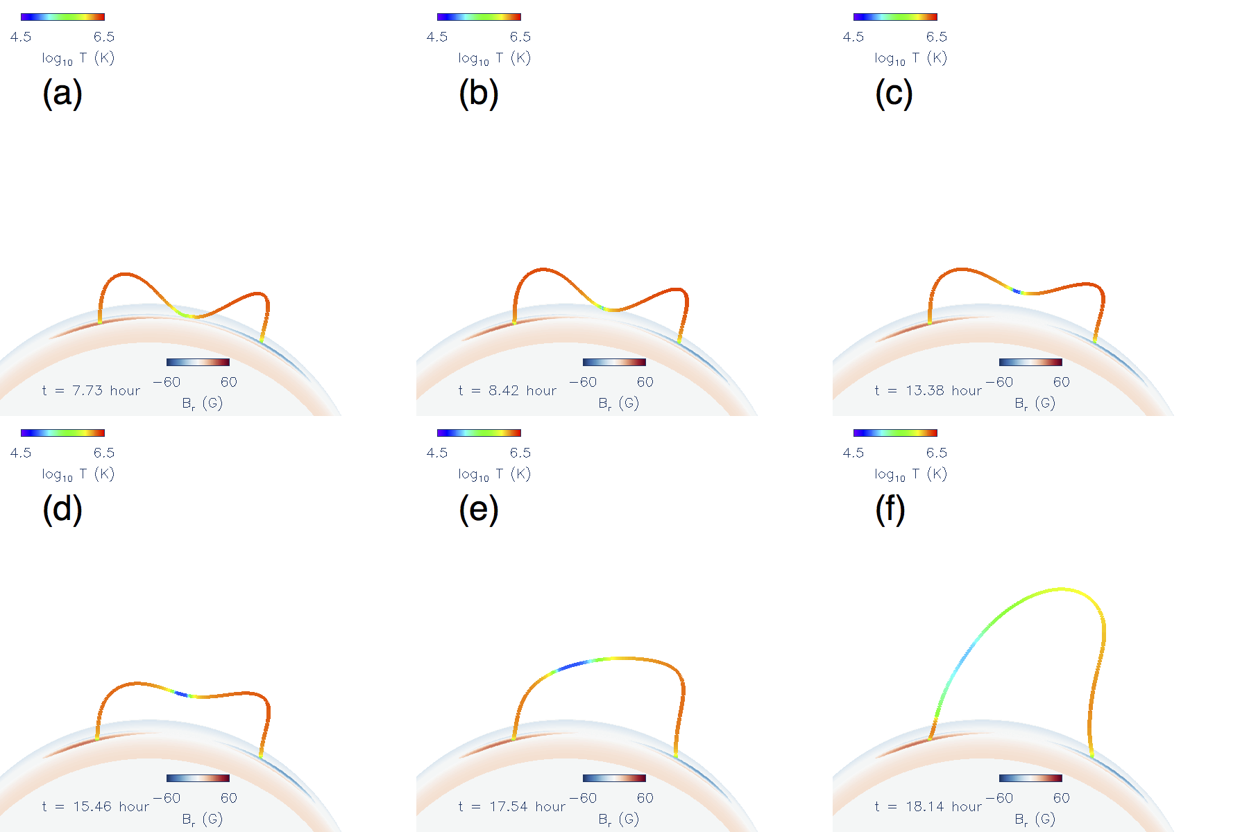
Figure 14: The evolution of a prominence carrying field line colored with temperature $T$. The lower boundary sphere is colored with $B_{r}$. A movie of this Figure showing the evolution from $t=6.14$ hour to $t=18.4$ hour is available in the online version.

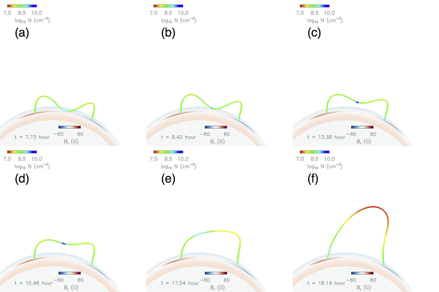
Figure 15: The same as Fig. 14 but the field line is colored with density. A movie of this Figure showing the evolution from $t=6.14$ hour to $t=18.4$ hour is available in the online version.

Figure 16 shows the evolution of temperature, density, and internal energy at the center of the dip of the tracked field line shown in Figures 14 and 15 from a time soon after the emergence of the dip to about the time it disappears due to the onset of eruption.

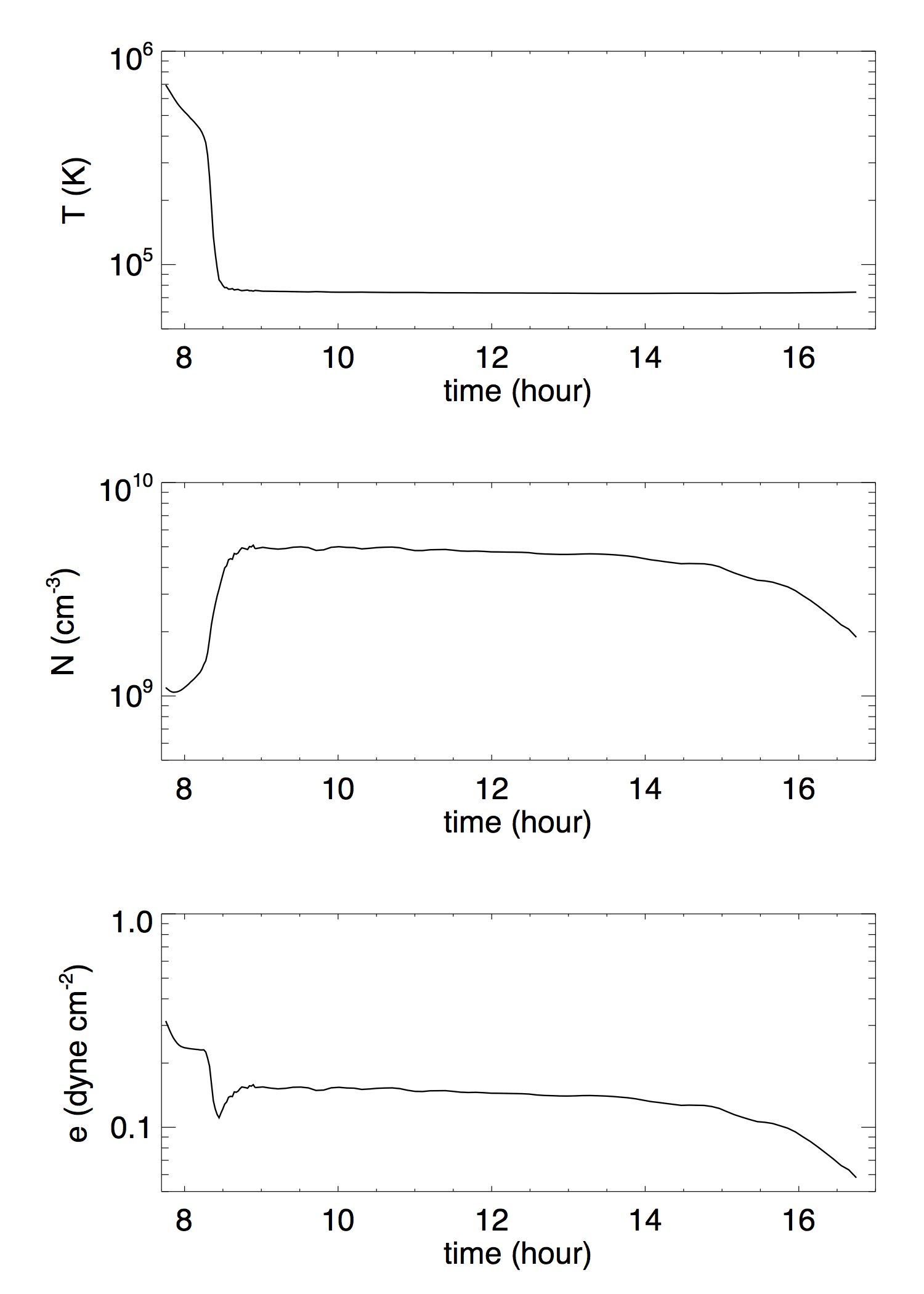
Figure 16: The evolution of temperature $T$, density $N$, and internal energy $e$ at the center of the dip of the tracked field line shown in Figures 14 and 15.

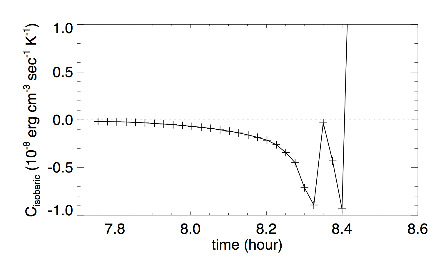
Figure 17: Evaluation of $C_{\rm isobaric}$ for the criterion for isobaric thermal instability at the center of the dip (see text).

We can see that soon after the emergence of the dip (Figures 14(a) and 15(a)), the plasma in the dip has a coronal temperature of about $7\times 10^{5}$ K and a density of about $1.1\times 10^{9}{\rm cm}^{-3}$, and it is already not in thermal equilibrium, showing a cooling with decrease in $T$ and $e$ (see top and bottom panels of Figure 16 at about $t=7.7$ hour). The density shows a brief initial decrease as an initial dynamic adjustment due to the rise of the dip and then shows a steady increase (middle panel of Figure 16 at about $t=7.7$ hour). At about $t=8.25$ hour, an even faster phase of cooling sets in with sharper decrease of temperature and pressure, and sharper increase of density, until about $t=8.6$ hour, when the dip settles into a thermal equilibrium for the rest of the time of the quasi-static phase. We have also evaluated the criterion for the isobaric thermal instability as given in Xia et al. (2011, and references therein):

$$C_{\rm isobaric}\equiv\rho\left(\frac{\partial L}{\partial T}\right)_{\rho}-\frac{\rho^{2}}{T}\left(\frac{\partial L}{\partial\rho}\right)_{T}+k^{2}\kappa<0,$$ (24)

where $L\equiv(Q-H)/\rho$ with $Q$ and $H$ given by equations 13 and 14 respectively, $\kappa=\kappa_{0}T^{5/2}$ is the thermal conductivity, and $k$ is the wavenumber for the thermal perturbation. Equation 24 is the criterion for the thermal instability assuming fixed pressure (isobaric), which is suitable under the condition that hydrostatic balance is maintained. We evaluate $C_{\rm isobaric}$ at the dip, where we use the width of the dip as the half wavelength for $k$, and estimate the width as the distance along the field line between the two points where $T$ has risen to twice the value at the bottom of the dip. We assume $H$ is unchanged since it is only a function of height. The result of $C_{\rm isobaric}$ is shown in Figure 17, where we find that the thermal instability criterion is met soon after the emergence from $t=7.7$ hour until about $t=8.4$, when $T$ at the dip has dropped to about $T=7.3\times 10^{4}$ K at which the steep decline of cooling function with decreasing temperature provides the strong stabilizing effect to suppress the instability. Thus the plasma at the dip is undergoing thermal non-equilibrium soon after the emergence and does not find an equilibrium until it cools down to about $7\times 10^{4}$ K. The sharper decrease of $T$ that sets in at about $t=8.25$ hour is due to the enhanced cooling as $\Lambda$ increases sharply with decreasing $T$ at $T$ $\sim 4\times 10^{5}$ K (see Figure 1) compounded by the increase in density. We also find that the cooling time scale (estimated from $e/Q$ at the dip) decreases to become comparable to the sound crossing time of the width of the dip at about this time ($t=8.25$ hour) which may be the cause of the onset of the sharper drop in $e$ or pressure, because the hydrostatic balance is no longer well maintained. Through the course of the thermal non-equilibrium, we find that the temperature at the dip drops from about $7\times 10^{5}$ K to about $T=7.3\times 10^{4}$ K, and remains there for the rest of the quasi-static rise phase (Figure 16 and panels (b), (c), (d) of Figure 14). The density increases from about $1.\times 10^{9}{\rm cm}^{-3}$ to a peak value of about $5\times 10^{9}{\rm cm}^{-3}$, and remains above about $3\times 10^{9}{\rm cm}^{-3}$ while the dip is present (Figure 16 and panels (b), (c), and (d) of Figures 15). When the dip disappears due to the onset of eruption the density drastically reduces and part of the condensation drains down along the left leg of the field line while part of the mass erupts with the top portion of the loop (panels (e) and (f) of Figures 14 and 15).

In our simulation we find that the peak density for the prominence condensation form in the coronal domain reaches about $5.6\times 10^{9}{\rm cm}^{-3}$, about 30 times the density of the surrounding coronal plasma. In the solar corona, the density ratio between the prominence and the surrounding corona can be more than 100 (e.g. see review in Priest, 2014). The reason that our simulation of the prominence condensation does not reach the observed density is most likely due to the imposed suppression of the radiative cooling for $T\leq 7\times 10^{4}$ K as shown in Figure 1, which prevents the temperature at the prominence dip from going below $7\times 10^{4}$ K. This prevents the pressure at the dip from dropping lower to draw more prominence mass from the field line foot points. It also limits how high the density can be increased for the same pressure at the dip. Furthermore, the way the lower boundary condition is imposed, where the radial velocity needs to accelerate from nearly zero from the lower boundary mass reservoir given the specified pressure may constrain the mass flow to the condensation at the dips.

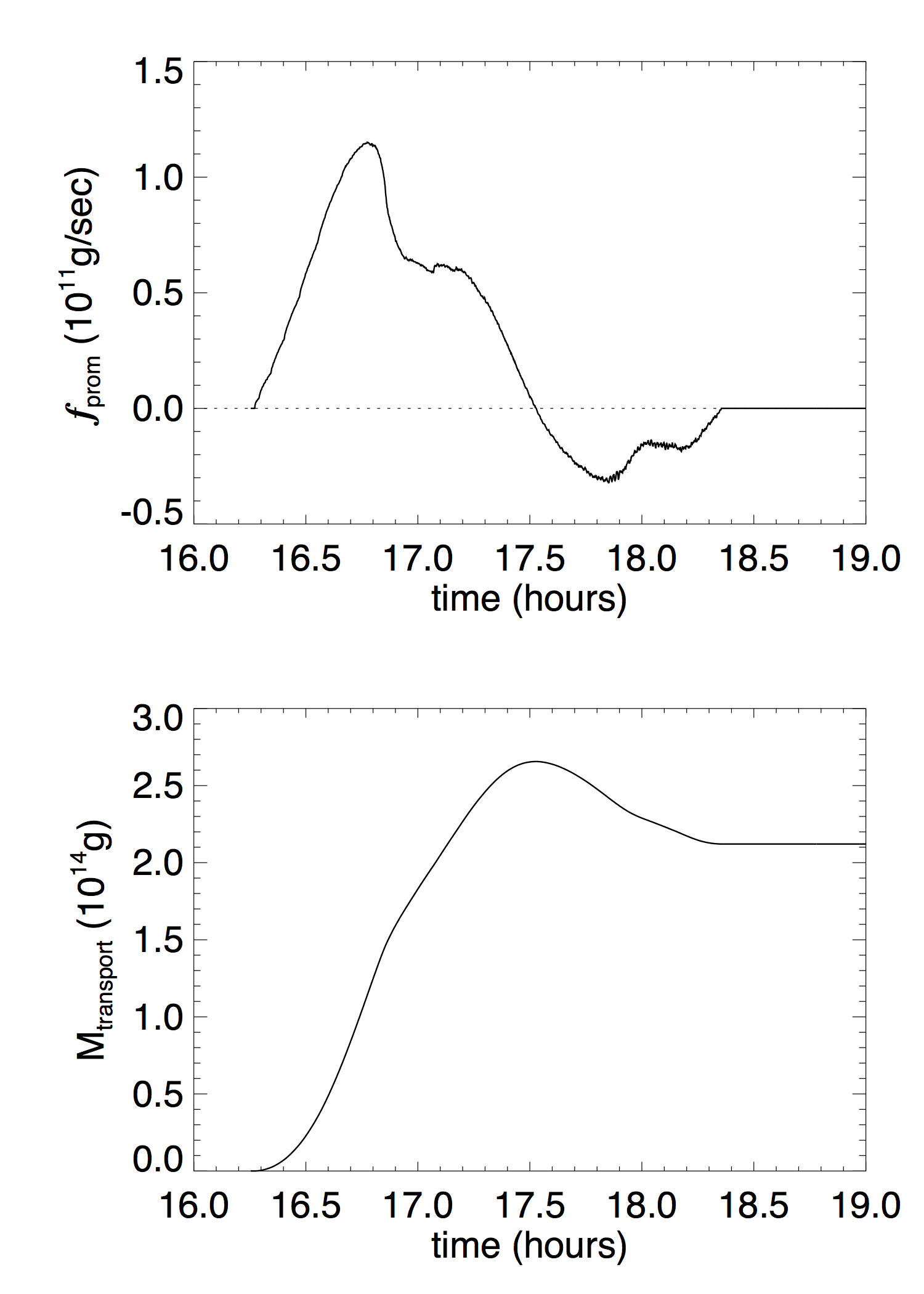
Figure 18: (top) The prominence mass flux and (bottom) the time integrated net prominence mass transported across the constant height surface at $r=1.264R_{\odot}$.

It is difficult to estimate the percentage of prominence mass that is ejected vs. drained down during the eruption because the temperature of the plasma is changing. Here we compute an integrated mass flux of cool prominence mass across a certain constant height surface. For this we consider cool prominence mass with temperature below $10^{5}$ K. We find that the total cool prominence mass in the coronal domain reaches a peak value of $M_{\rm peak}=5.46\times 10^{14}g$ at time $t_{\rm peak}=16.3$ hours, with the prominence apex reaching the height of $r_{\rm peak}=1.264R_{\odot}$. Then starting from $t_{\rm peak}$ we compute the prominence mass flux $f_{\rm prom}=\int(\rho v_{r})_{T<10^{5}K}dS$ through the constant height surface $S$ at $r_{\rm peak}$ and integrate this flux over time to obtain the net prominence mass transport through S over time: $M_{\rm transport}(t)=\int_{t_{\rm peak}}^{t}f_{\rm prom}dt$. The result for $f_{\rm prom}$ and $M_{\rm transport}$ are shown in Figure 18. We see an outward prominence flux $f_{\rm prom}$ from $t_{\rm peak}=1.63$ hours to $t\approx 17.5$ hours, and an inward flux $f_{\rm prom}$ from $t\approx 17.5$ hours to $t\approx 18.36$ hours, after which there is no more flux of cool prominence material. Thus the net prominence mass transport $M_{\rm transport}$ out of the surface $S$ at $r_{\rm peak}$ reaches a final value of about $2.1\times 10^{14}$ g, which is about 40% of the peak prominence mass formed below $S$. However there is uncertainty with this estimate because the prominence material could have heat up to above $10^{5}$ K before rising through (or falling through) the surface S, which would result in under estimating (over estimating) the erupted prominence mass. For this estimate we are only taking into account net transport of mass that remains below $T$ of $10^{5}$ K.

We find that in the field line dips of the flux rope where the prominence condensations form, the magnetic field becomes significantly non-force-free because of the prominence weight. Figure 19 shows the various radial forces (top), density (middle), and total magnetic field strength (bottom) along the central vertical line through the middle of the flux rope shown in Figure 5(c). The vertical line also goes through the middle of the prominence carrying field lines shown in Figure 12(b).

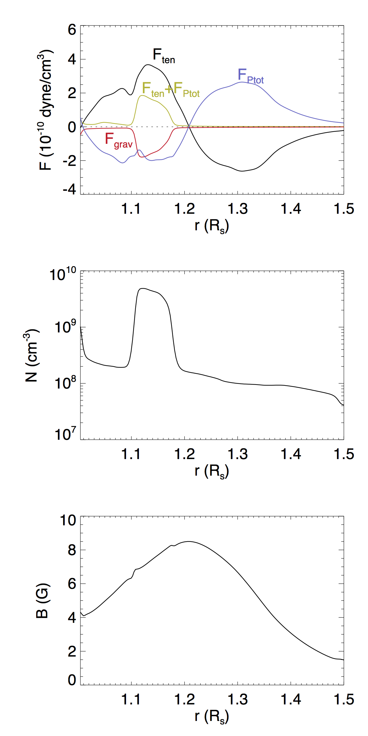
Figure 19: Radial forces (top), density (middle), and total magnetic field strength (bottom) along the central vertical line through the middle of the flux rope shown in Figure 5(c). It also goes through the middle of the prominence carrying field lines shown in Figure 12(b). The radial forces shown in the top panel are the magnetic tension force $F_{\rm ten}$ (black curve), the total pressure gradient force $F_{\rm Ptot}$ (blue curve), where the total pressure is mostly made up of the magnetic pressure, the sum $F_{\rm ten}+F_{\rm Ptot}$ (green curve), which is approximately the net Lorentz force, and the gravity force of the plasma $F_{\rm grav}$ (red curve).

We can see from Figure 19 that in the height range where the prominence has formed (indicated by the high density bump in the middle panel), the downward gravity $F_{\rm grav}$ (red curve in the upper panel) of the prominence plasma counteracts a significant portion of the upward tension force $F_{\rm ten}$ (black curve in the upper panel) of the magnetic field. In the flux rope the magnetic tension $F_{\rm ten}$ and the total pressure gradient $F_{\rm Ptot}$ (where the total pressure is largely made up of the magnetic pressure) are well balanced and hence force-free outside of the prominence carrying region, as can be seen by comparing the black and the blue curves in the top panel. The sum $F_{\rm ten}+F_{\rm Ptot}$ (green curve), which is approximately the net Lorentz force, is nearly zero except in the prominence carrying region, where it has a significant positive net force to counteract the downward gravity force. Thus despite the fact that the plasma $\beta$ is low throughout the flux rope (about 0.01 to 0.1 in the prominence region), the magnetic field is significantly non-force-free in the region of the prominence, where the prominence weight is counteracting a major portion of the upward magnetic tension, with the remainder balanced by the downward magnetic pressure gradient force. Note that the magnetic pressure gradient force (blue curve) is downward in the prominence region to counteract partly the upward tension, changing sign in the upper part of the flux rope where the curvature changes sign. Thus the magnetic field strength is increasing with height in the prominence (see lower panel of Figure 19). This would be an observational signature from prominence magnetic field measurement that indicates that the prominence is associated with dipped or concave upturning magnetic field lines. Our result on the significantly non-force-free field in low-$\beta$ plasma supporting the weight of the prominence in the field line dips is consistent with the findings in previous MHD models of prominences by (Xia et al., 2012) and Hillier & van Ballegooijen (2013).

4 Discussion

We have improved upon previous simulations of flux rope destabilization and eruption by using a helmet streamer pre-existing coronal field, and incorporating a more sophisticated treatment of the thermodynamics that explicitly include the non-adiabatic effects: an empirical coronal heating, optically thin radiative losses, and field-aligned thermal conduction. Depending on the size of the pre-existing streamer, we find different scenarios and mechanisms for the transition from quasi-equilibrium to ejective eruption for the flux rope. For a broad streamer with a slow decline of the magnetic field with height, the flux rope is found to remain well confined until its emerged twist is sufficiently high for the kink instability to set in first. The kinked flux rope can still remain confined and goes through a quasi-static, slow rise phase until its kinked apex reaches a certain height with sufficient decline of the confining field where it develops a “hernia-like” ejective eruption. On the other hand with a narrow streamer with a steeper decline of the field with height, the flux rope can erupt with a twist that is significantly below the onset of the kink instability. It undergoes a quasi-static rise phase where tether-cutting reconnections convert arcade flux into twisted flux of the flux rope, reducing the confinement, and develops an ejective eruption when it reaches the critical height for the onset of the torus instability. The above mechanisms for the onset of eruption are in qualitatively agreement with previous findings in simulations using a potential pre-existing field and with simplified treatment of the thermodynamics (e.g. Török & Kliem, 2005; Fan & Gibson, 2007; Aulanier et al., 2010; Fan, 2010). Our simulations confirm that the fast decay with height of the confining helmet magnetic field is a key factor for achieving an ejective eruption of the underlying flux rope. Our simulations also show that with the more realistic adiabatic index of $\gamma=5/3$, which produces a stronger adiabatic cooling of the expanding erupting flux rope, and with an explicit treatment of the heating and heat transport, the erupting flux rope is still able to accelerate to a typical CME terminal speed ($\sim 600$ km/s in our ejective eruption cases) in excess of the ambient solar wind speed.

We have also achieved a simulation of the prominence eruption. With the explicit inclusion of the optically thin radiative losses, we found the formation of prominence condensations with a temperature as low as $7.3\times 10^{4}$ K and density as high as $5.6\times 10^{9}{\rm cm}^{-3}$ in the field line dips of the significantly twisted flux ropes (in the WS-L and WS-M cases) during the quasi-static phase. The prominence condensations are formed in the field line dips after the emergence into the corona, as a result of the onset of radiative instability or non-equilibrium. The prominence condensations develop into an elongated structure suspended in the corona as viewed in SDO/AIA 304 Å emission. The elongated prominence structure makes an acute angle of about $30^{\circ}$ with the orientation of the field lines supporting the prominence, consistent with observations. However, once formed due to runaway radiative cooling, the pressure scale height of the coolest part of the prominence condensations (reaching a minimum of 4.4 Mm) is only resolved by about 2 grid points given our numerical resolution and hence not well resolved. Thus their evolution is likely significantly impacted by numerical diffusion and is probably reflecting an averaged collective motion of the condensations. We find that because of the weight of the prominence condensations that formed, the prominence carrying field becomes significantly non-force-free (despite being low plasma $\beta$) with a significant fraction of the magnetic tension force counteracting the gravity force of the prominence, and with the remainder upward tension force of the concave field lines balanced by a downward magnetic pressure gradient force. This confirms the previous findings by Xia et al. (2012) and Hillier & van Ballegooijen (2013). Thus the formation of the prominence may be playing a significant role in increasing the confinement of the flux rope.

With the eruption of the flux rope in the WS-L case and the disappearance of the dips, we find that the prominence plasma shows substantial draining along the legs of the erupting field lines, developing into an erupting loop structure as viewed in AIA 304 Å emission. The erupting prominence obtained here does not show a kinked morphology, even though the flux rope becomes significantly kinked when viewed from the same perspective. We find that the cool prominence condensation (with $T<10^{5}$ K) reaches a peak mass of about $5.46\times 10^{14}g$ in the corona and estimate that roughly 40% of the cool prominence mass is transported out with the eruption. These results on the evolution of the prominence need to be further investigated with higher resolution simulations that better resolve the prominence condensations that develop.

In the case with the shorter, less twisted flux rope (NS-S case), which eventually erupts due to the onset of the torus instability, we do not find the formation of prominence condensations. Instead we find the formation of a sigmoid-shaped hot channel which contains heated, twisted flux added to the flux rope as a results of tether-cutting reconnections during the quasi-static rise phase. This thermal signature of tether-cutting reconnection may explain the hot channels observed by SDO/AIA before and during the onset of CMEs as described in e.g. Zhang et al. (2012) and Cheng et al. (2013). However to quantitatively produce the observed temperature of the hot channels (about 10 MK) so as to be able to model the bright emissions of the hot channels seen in AIA 131 Å and AIA 94 Å images, simulations with a significantly increased field strength for the flux rope and the confining helmet streamer are needed.

References

- Amari et al. (2014) Amari, T., Canou, A., & Aly, J.-J. 2014, Nature, 514, 465
- Antiochos et al. (1999) Antiochos, S. K., DeVore, C. R., & Klimchuk, J. A. 1999, ApJ, 510, 485
- Athay (1986) Athay, R. G. 1986, ApJ, 308, 975
- Aulanier et al. (2010) Aulanier, G., Török, T., Démoulin, P., & DeLuca, E. E. 2010, ApJ, 708, 314
- Bommier et al. (1994) Bommier, V., Landi Degl’Innocenti, E., Leroy, J.-L., & Sahal-Brechot, S. 1994, Sol. Phys., 154, 231
- Chatterjee & Fan (2013) Chatterjee, P., & Fan, Y. 2013, ApJ, 778, L8
- Cheng et al. (2013) Cheng, X., Zhang, J., Ding, M. D., Liu, Y., & Poomvises, W. 2013, ApJ, 763, 43
- Démoulin & Aulanier (2010) Démoulin, P., & Aulanier, G. 2010, ApJ, 718, 1388
- Downs et al. (2012) Downs, C., Roussev, I. I., van der Holst, B., Lugaz, N., & Sokolov, I. V. 2012, ApJ, 750, 134
- Fan (2010) Fan, Y. 2010, ApJ, 719, 728
- Fan (2012) —. 2012, ApJ, 758, 60
- Fan (2016) —. 2016, ApJ, 824, 93
- Fan & Gibson (2007) Fan, Y., & Gibson, S. E. 2007, ApJ, 668, 1232
- Gibson (2015) Gibson, S. 2015, in Astrophysics and Space Science Library, Vol. 415, Solar Prominences, ed. J.-C. Vial & O. Engvold, 323
- Gombosi et al. (2002) Gombosi, T. I., Tóth, G., De Zeeuw, D. L., et al. 2002, Journal of Computational Physics, 177, 176
- Hillier & van Ballegooijen (2013) Hillier, A., & van Ballegooijen, A. 2013, ApJ, 766, 126
- Hollweg (1978) Hollweg, J. V. 1978, Reviews of Geophysics and Space Physics, 16, 689
- Hood & Priest (1981) Hood, A. W., & Priest, E. R. 1981, Geophysical and Astrophysical Fluid Dynamics, 17, 297
- Isenberg & Forbes (2007) Isenberg, P. A., & Forbes, T. G. 2007, ApJ, 670, 1453
- Kliem & Török (2006) Kliem, B., & Török, T. 2006, Physical Review Letters, 96, 255002
- Landi et al. (2012) Landi, E., Del Zanna, G., Young, P. R., Dere, K. P., & Mason, H. E. 2012, ApJ, 744, 99
- Leroy et al. (1983) Leroy, J. L., Bommier, V., & Sahal-Brechot, S. 1983, Sol. Phys., 83, 135
- Linker et al. (2007) Linker, J. A., Lionello, R., Mikic, Z., Riley, P., & Titov, V. 2007, in Bulletin of the American Astronomical Society, Vol. 39, American Astronomical Society Meeting Abstracts #210, 168
- Low (2001) Low, B. C. 2001, J. Geophys. Res., 106, 25141
- Mackay & van Ballegooijen (2006) Mackay, D. H., & van Ballegooijen, A. A. 2006, ApJ, 641, 577
- Meyer et al. (2012) Meyer, C. D., Balsara, D. S., & Aslam, T. D. 2012, MNRAS, 422, 2102
- Orozco Suárez et al. (2014) Orozco Suárez, D., Asensio Ramos, A., & Trujillo Bueno, J. 2014, A&A, 566, A46
- Pagano et al. (2014) Pagano, P., Mackay, D. H., & Poedts, S. 2014, A&A, 568, A120
- Pagano et al. (2015) —. 2015, Journal of Astrophysics and Astronomy, 36, 123
- Priest (2014) Priest, E. 2014, Magnetohydrodynamics of the Sun (Cambridge, UK: Cambridge University Press)
- Rempel (2017) Rempel, M. 2017, ApJ, 834, 10
- Rempel et al. (2009) Rempel, M., Schüssler, M., & Knölker, M. 2009, ApJ, 691, 640
- Stone & Norman (1992) Stone, J. M., & Norman, M. L. 1992, ApJS, 80, 791
- Titov & Démoulin (1999) Titov, V. S., & Démoulin, P. 1999, A&A, 351, 707
- Török & Kliem (2005) Török, T., & Kliem, B. 2005, ApJ, 630, L97
- Török & Kliem (2007) —. 2007, Astronomische Nachrichten, 328, 743
- Török et al. (2011) Török, T., Panasenco, O., Titov, V. S., et al. 2011, ApJ, 739, L63
- van der Holst et al. (2014) van der Holst, B., Sokolov, I. V., Meng, X., et al. 2014, ApJ, 782, 81
- Webb & Hundhausen (1987) Webb, D. F., & Hundhausen, A. J. 1987, Sol. Phys., 108, 383
- Withbroe (1988) Withbroe, G. L. 1988, ApJ, 325, 442
- Xia et al. (2012) Xia, C., Chen, P. F., & Keppens, R. 2012, ApJ, 748, L26
- Xia et al. (2011) Xia, C., Chen, P. F., Keppens, R., & van Marle, A. J. 2011, ApJ, 737, 27
- Xia & Keppens (2016) Xia, C., & Keppens, R. 2016, ApJ, 823, 22
- Xia et al. (2014) Xia, C., Keppens, R., Antolin, P., & Porth, O. 2014, ApJ, 792, L38
- Zhang et al. (2012) Zhang, J., Cheng, X., & Ding, M.-D. 2012, Nature Communications, 3, arXiv:1203.4859