Quantum transduction with adaptive control

Abstract

Quantum transducers play a crucial role in hybrid quantum networks. A good quantum transducer can faithfully convert quantum signals from one mode to another with minimum decoherence. Most investigations of quantum transduction are based on the protocol of direct mode conversion. However, the direct protocol requires the matching condition, which in practice is not always feasible. Here we propose an adaptive protocol for quantum transducers, which can convert quantum signals without requiring the matching condition. The adaptive protocol only consists of Gaussian operations, feasible in various physical platforms. Moreover, we show that the adaptive protocol can be robust against imperfections associated with finite squeezing, thermal noise, and homodyne detection. It can be implemented to realize quantum state transfer between microwave and optical modes.

Quantum transducers (QT) can convert quantum signals from one bosonic mode to another, which may have different frequencies, polarizations, or even mode carriers. QT enables quantum information transfer between different physical platforms, which is crucial for hybrid quantum networks (Kimble, 2008; Duan and Monroe, 2010). There have been significant advances toward quantum state transfer between different bosonic systems, such as conversion between microwave and mechanical/spin-wave modes (Palomaki et al., 2013; Zhang et al., 2014; Tabuchi et al., 2015), between optical and mechanical/spin-wave modes (Lukin, 2003; Hammerer et al., 2010; Safavi-Naeini and Painter, 2011; Aspelmeyer et al., 2014a), and etc. Motivated by the hybrid quantum networks with optical quantum communication and microwave quantum information processing, recently there are experimental demonstrations of coherent conversion between microwave and optical signals with decent conversion efficiencies (Andrews et al., 2014; Vainsencher et al., 2016; Fong et al., 2014), but the signal attenuation and added noise still prevent us from achieving quantum transduction between microwave and optical modes.

Most investigations of quantum transduction are based on the direct quantum transduction (DQT) protocol. As illustrated in Fig. 1(a), QDT protocol has a simple structure that injects quantum signals to the input port and retrieves them from the output port of the mode converter, which can hybridize different modes with enhanced bilinear couplings betweeen localized modes (Fig. 1(b)). The energy mismatch between the input and output states can be compensated by parametric processes and stiff pumps (Pelc et al., 2012; Abdo et al., 2013; Andrews et al., 2014; Vainsencher et al., 2016; Guo et al., 2016). Unlike classical signals, quantum signals are vulnerable to both attenuation and amplification, which irreversibly add noise and induce decoherence. Hence, DQT protocol requires the matching condition (MC) — the subblock of the scattering matrix associated with the input and output ports should be equivalent to the identity matrix — so that every excitation entering the input port can be faithfully converted into an excitation exiting the output port, without affecting other ports (Safavi-Naeini and Painter, 2011; Wang and Clerk, 2012; Kurizki et al., 2015). In practice, however, MC is not always feasible, due to limited tunability of device parameters (Aspelmeyer et al., 2014b) and undesired parametric conversion processes (Andrews et al., 2014). For small deviation from MC, we may use quantum error correction to actively suppress the noise and restore the encoded quantum information (Cochrane et al., 1999; Gottesman et al., 2001; Leghtas et al., 2013; Mirrahimi et al., 2014; Michael et al., 2016; Xiang et al., 2017; Vermersch et al., 2017; Ofek et al., 2016). Nevertheless, the quantum error correction has limited capability of correcting errors (e.g., no more than 50% loss) (Bennett et al., 1997). Therefore, it is important to develop a quantum transduction protocol to bypass MC.

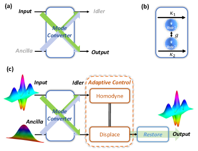
Figure 1: Schematic of the direct and adaptive protocols. (a) The direct protocol injects quantum signals to the input port and retrieves them from the output port of the mode converter. (b) A simple mode converter has bilinear coupling $\hat{H}=\left(ga_{1}^{\dagger}a_{2}+g^{\prime}a_{1}^{\dagger}a_{2}^{\dagger}+h.c\right)$ between two internal modes $a_{1}$ and $a_{2}$ with coupling strengths $g$ and $g^{\prime}$, and external coupling strength $\kappa_{1}$ and $\kappa_{2}$. (c) The adaptive protocol injects not only quantum signals to the input port, but also squeezed vacuum to the ancilla port of the mode converter. The adaptive control (dashed orange box) performs a displacement operation to the output port conditioned on the homodyne detection of the idler port. Up to a unitary recovery operation (cyan box), quantum signals can be retrieved from the output port.

In this Letter, we propose the adaptive quantum transduction (AQT) protocol that does not require MC. Adaptive quantum protocols have been developed for various applications, including quantum teleportation (Bouwmeester et al., 1997; Furusawa et al., 1998), quantum phase estimation (Higgins et al., 2007), measurement based quantum computation (Raussendorf and Briegel, 2001; Menicucci et al., 2006), and quantum error correction (Nielsen and Chuang, 2000), etc. We incorporate the ingredients of adaptive control to the general design of quantum transducers to bypass MC as well as boost the performance.

Adaptive quantum transduction.

As illustrated in Fig. 1(c), AQT prepares a squeezed vacuum for the ancilla port, performs homodyne detection at the idler port, and applies adaptive control to the output conditioned on the homodyne outcome. Up to a unitary operation, quantum signals can be converted from the input to output ports. If MC is satisfied, quantum signals can be perfectly converted with no need of adaptive control, and thus AQT is reduced to DQT (Fig. 1(a)). If MC is not fulfilled, the mode converter will distribute the quantum signal (gray arrow) and squeezed vacuum noise (curved arrow) over both output and idler ports. The quantum signal leaks into the environment via the idler port, while the noise is added to the output. However, the squeezed vacuum from ancilla port injects a strong and correlated noise to the anti-squeezing quadratures of the output and idler ports, so that we may use homodyne detection and adaptive control to cancel the added noise as well as prevent the signal leakage to the environment. On the one hand, the homodyne detection measures the anti-squeezed noises of the idler port without disclosing the information about the quantum signal, since the idler port is dominated by the large fluctuation of the anti-squeezed noise. On the other hand, the adaptive displacement operation conditioned on the homodyne detection completely removes the correlated anti-squeezing noise of the output port, leaving the output signal equivalent to the input signal up to a Gaussian unitary operation. Since there is no assumption of prior-knowledge of the input signal, the protocol can faithfully convert arbitrary quantum signal from one mode to another.

Generally, we consider a mode converter that transforms $m$ input modes and $n$ ancilla modes into $m$ output modes and $n$ idler modes. AQT protocol will (1) inject squeezed vacuum $\hat{\rho}_{anc}$ to the ancilla modes, (2) perform homodyne measurement $\hat{\Pi}_{\eta}$ for the idler modes with outcome $\mathbf{\eta}\in\mathbb{R}^{n}$, and (3) apply adaptive displacement $\mathcal{D}_{\mathbf{F}\mathbf{\mathbf{\eta}}}$ to the output modes with linearly transformed displacement $\mathbf{F}\mathbf{\mathbf{\eta}}\in\mathbb{C}^{m}$. For arbitrary input state $\hat{\rho}_{in}$, the output state of AQT is

$$\hat{\rho}_{out}=\int d\mathbf{\eta}\mathcal{D}_{\text{$\mathbf{F}\mathbf{\eta}$}}\left[\mathrm{tr}_{\mathrm{meas}}(\mathcal{U}_{\mathbf{S}}\left[\hat{\rho}_{in}\otimes\hat{\rho}_{anc}\right]\hat{\Pi}_{\eta})\right],$$ (1)

where $\mathcal{U}_{\mathbf{S}}$ is the Gaussian unitary operation (Weedbrook et al., 2012) from the mode converter, which can be characterized by a symplectic scattering matrix $\mathbf{S}$ transforming the input and ancilla modes ($\mathbf{x}$) to the output and idler modes ($\mathbf{y}$)

$$\left(\begin{array}[]{c}\mathbf{y}{}_{b}\\ \mathbf{y}{}_{b^{\prime}}\\ \mathbf{y}{}_{h}\\ \mathbf{y}{}_{h^{\prime}}\end{array}\right) = \left(\begin{array}[]{cccc}\mathbf{S}_{b,a}&\mathbf{S}_{b,a^{\prime}}&\mathbf{S}_{b,z}&\mathbf{S}_{b,z^{\prime}}\\ \mathbf{S}_{b^{\prime},a}&\mathbf{S}_{b^{\prime},a^{\prime}}&\mathbf{S}_{b^{\prime},z}&\mathbf{S}_{b^{\prime},z^{\prime}}\\ \mathbf{S}_{h,a}&\mathbf{S}_{h,a^{\prime}}&\mathbf{S}_{h,z}&\mathbf{S}_{h,z^{\prime}}\\ \mathbf{S}_{h^{\prime},a}&\mathbf{S}_{h^{\prime},a^{\prime}}&\mathbf{S}_{h^{\prime},z}&\mathbf{S}_{h^{\prime},z^{\prime}}\end{array}\right)\left(\begin{array}[]{c}\mathbf{x}_{a}\\ \mathbf{x}_{a^{\prime}}\\ \mathbf{\mathbf{x}}_{z}\\ \mathbf{x}_{z^{\prime}}\end{array}\right),$$ (14)

with $\mathbf{x}_{a}(\mathbf{x}_{a^{\prime}})$ for all the Q(P)-quadratures of the input modes, $\mathbf{y}{}_{b}(\mathbf{y}{}_{b^{\prime}})$ for the Q(P)-quadratures of the output modes, $\mathbf{x}_{z(z^{\prime})}$ for the squeezed (anti-squeezed) quadratures of the ancillary modes, and $\mathbf{y}_{h(h^{\prime})}$ for the measured (unmeasured) quadratures of the idler modes. MC corresponds to a special case that the subblock $\begin{pmatrix}\mathbf{S}_{b,a}&\mathbf{S}_{b,a^{\prime}}\\ \mathbf{S}_{b^{\prime},a}&\mathbf{S}_{b^{\prime},a^{\prime}}\end{pmatrix}$ of the scattering matrix is equivalent to the identity matrix up to some symplectic transformation (Safavi-Naeini and Painter, 2011; Wang and Clerk, 2012; SM, ), but here we do not require such a condition for AQT. We may choose the squeezed and measured quadratures ($\mathbf{x}_{z}$ and $\mathbf{y}_{h}$), so that the anti-squeezed noise in $\mathbf{x}_{z^{\prime}}$ can be inferred from the homodyne detection of $\mathbf{y}_{h}$ associated with an invertible submatrix $\mathbf{S}_{h,z^{\prime}}$. We choose the linear transformation

$$\mathbf{F}=\mathbf{F}_{\star}=-\begin{pmatrix}\mathbf{S}_{b,z^{\prime}}\\ \mathbf{S}_{b^{\prime},z^{\prime}}\end{pmatrix}\left(\mathbf{S}_{h,z^{\prime}}\right)^{-1},$$ (15)

which can completely remove the anti-squeezed noise from the output modes. Moreover, for this particular choice of $\mathbf{F}_{\star}$, the effective scattering matrix between the input and output is

$$\tilde{\mathbf{S}} = \begin{pmatrix}\mathbf{S}_{b,a}&\mathbf{S}_{b,a^{\prime}}\\ \mathbf{S}_{b^{\prime},a}&\mathbf{S}_{b^{\prime},a^{\prime}}\end{pmatrix}+\mathbf{F}_{\star}\begin{pmatrix}\mathbf{S}_{h,a}&\mathbf{S}_{h,a^{\prime}}\end{pmatrix},$$ (16)

which is a symplectic matrix, as shown in Theorem 1 of (SM, ). Unlike general scattering matrices, the symplectic $\mathbf{\tilde{S}}$ implies that the output state (after the adaptive displacement) is a simple Gaussian unitary transformation of the input state

$$\hat{\rho}_{out}=\mathcal{U}_{\tilde{\mathbf{S}}}\left[\hat{\rho}_{in}\right],$$ (17)

where $\mathcal{U}_{\tilde{\mathbf{S}}}$ is the Gaussian unitary operation associated with symplectic $\mathbf{\tilde{S}}$. We can perfectly restore the original input state by applying a unitary recovery operation $\mathcal{U}_{\tilde{\mathbf{S}}}^{-1}$ over the output modes, $\hat{\rho}_{out}\rightarrow\mathcal{U}_{\tilde{\mathbf{S}}}^{-1}\left[\hat{\rho}_{out}\right]=\hat{\rho}_{in}$. Since AQT protocol works for generic scattering matrix $\mathbf{S}$, it can bypass MC to achieve perfect conversion of arbitrary quantum signals.

Finte squeezing and imperfect homodyne.

So far, we have assumed the ideal situation with infinite squeezing and perfect homodyne detection for AQT protocol. In practice, however, we only have finite squeezing and imperfect homodyne detection. The finite squeezing can be characterized by $\nu=e^{-2\xi}(2n_{z}+1)$, depending on the squeezing parameter $\xi$ and thermal noise $n_{z}$ prior to squeezing. In terms of logorithmic unit of decibel, $x\rightarrow 10\log_{10}x~{}(\mathrm{dB})$, squeezing of $\nu\approx-15\mathrm{dB},-10\mathrm{dB}$ for optical and microwave modes have been achieved (Castellanos-Beltran et al., 2008; Eberle et al., 2010), respectively. The imperfect homodyne detection can be characterized by $\mu=\frac{1-\eta}{\eta}$, depending on the detector efficiency $\eta\leq 1$ . In terms of decibel , we can achieve homodyne detection with achievable imperfection of $\mu\approx-14\mathrm{dB},-0.1\mathrm{dB}$ for optical and microwave modes have been demonstrated (Fuwa et al., 2015; Mallet et al., 2011; Kindel et al., 2016), respectively. Since these imperfections can be characterized by Gaussian operations, AQT protocol with imperfections is still a Gaussian channel, which preserves the Gaussian character of a Gaussian state (Weedbrook et al., 2012). With the choice of $\mathbf{F}=\eta^{-1/2}\mathbf{F}_{\star}$, AQT protocol combined with the recovery operation $\mathcal{U}_{\tilde{\mathbf{S}}}^{-1}$ is effectively a classical-noise channel (Holevo, 2007; Weedbrook et al., 2012), which transforms the quadratures as $\left(\mathbf{x}_{a},\mathbf{x}_{a^{\prime}}\right)\rightarrow\left(\mathbf{x}_{a}+\xi,\mathbf{x}_{a^{\prime}}+\xi^{\prime}\right)$. The added noise $\left(\xi,\xi^{\prime}\right)$ is characterized by a $2m\times 2m$ covariance matrix (SM, )

$$\mathbf{V}=\nu\mathbf{B}_{\star}\mathbf{B}_{\star}^{T}+\mu\tilde{\mathbf{S}}^{-1}\mathbf{F}_{\star}\mathbf{F}_{\star}^{T}\left(\tilde{\mathbf{S}}^{-1}\right)^{T},$$ (18)

with $\mathbf{B}_{\star}=\begin{pmatrix}\left(\mathbf{S}^{-1}\right)_{a,h^{\prime}}\\ \left(\mathbf{S}^{-1}\right)_{a^{\prime},h^{\prime}}\end{pmatrix}\left[\left(\mathbf{S}^{-1}\right)_{z,h^{\prime}}\right]^{-1}$ . Note that $\mathbf{V}$ vanishes when $\nu\rightarrow 0$ (infinite squeezing) and $\mu\rightarrow 0$ (perfect homodyne detection), in correspondence with for the perfect conversion with the ideal AQT.

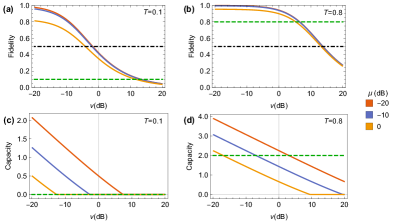
Figure 2: Performance of adaptive protocol with imperfect squeezing and homodyne detection. (a) & (b), The average fidelity of AQT as a function of imperfect squeezing $\nu$, given imperfect homodyne detection of $\mu=-20,-10$ and $0$dB for transmittance $T=0.8$ and $T=0.1$, respectively. The dark dotted dashed lines correspond to the threshold fidelity of $1/2$. The green dashed lines correspond to the fidelity achieved by DQT. (c) & (d), The quantum channel capacity of AQT for transmittance $T=0.8$ and $T=0.1$, respectively. The green dashed lines correspond to the channel capacity achieved by DQT. For $T=0.1$, the channel capacity vanishes for DQT, while AQT can achieve a finite quantum channel capacity with experimentally feasible $\mu$ and $\nu$.

Performance of adaptive protocol.

We use two criteria to evaluate the performance of AQT in the presence of imperfections — (1) the average fidelity between input and output over uniformly distributed coherent states (Braunstein et al., 2001; fn, 2) and (2) quantum channel capacity characterizing the amount of quantum information transmitted (Holevo and Werner, 2001; Harrington and Preskill, 2001; Pirandola et al., 2009). It is sufficient (not necessary) to demonstrate quantum transduction, if we have above-threshold average fidelity (>1/2) or quantum channel capacity (>0).

For example, we consider the minimum AQT with $m=1$ input (output) and $n=1$ ancilla (idler) modes, which is based on a converter with beam-splitter type coupling [e.g., $\hat{H}=g\left(a_{1}^{\dagger}a_{2}+h.c.\right)$]. We may simply use the transmittance $T\in\left[0,1\right]$ to characterize such a converter. Given fixed measurement imperfection ($\mu=0,-10$ or $-20$dB), the average fidelity decreases for larger squeezing imperfection ($\nu$) as shown in Fig. 2(a),(b) for different $T=0.8$ and $T=0.1$, respectively. For feasible squeezing ($\nu\lesssim 0$dB), AQT can outperform DQT (green curves) and exceed the threshold fidelity of 0.5 (dark dotted dashed lines) (Braunstein et al., 2001; fn, 3). We can also compute the quantum channel capacity versus squeezing imperfection as shown in Fig. 2(c),(d) for $T=0.8$ and $T=0.1$, respectively. When the transmittance is low ($T<0.5$), DQT is an anti-degradable channel with zero quantum channel capacity (Caruso and Giovannetti, 2006), while AQT can still achieve a finite quantum channel capacity when $\mu\nu<\frac{4}{9\left(T+1/T-2\right)}$ (SM, ).

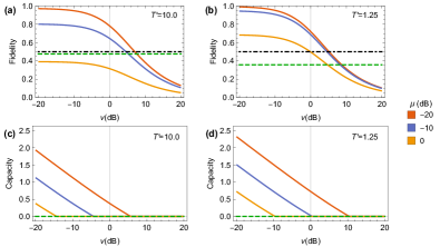
Figure 3: Performance of adaptive protocol with imperfect squeezing and homodyne detection. (a) & (b), Input-output fidelity of AQT protocol averaged over all coherent states as a function of imperfect squeezing $\nu$, given imperfect homodyne detection of $\mu=-20,-10$ and $0$dB for transmittance $T^{\prime}=1.25$ and $T^{\prime}=10.0$, respectively. The dark dotted dashed lines correspond to the threshold fidelity of $1/2$. The green dashed lines correspond to the fidelity achieved by DQT protocol. (c) & (d), The quantum channel capacity for transmittance $T^{\prime}=1.25$ and $T^{\prime}=10.0$, respectively. The channel capacity vanishes for DQT protocol shown by green dashed lines.

We also investigated AQT based on a converter with two-mode-squeezer type coupling [e.g., $\hat{H}=g\left(a_{1}^{\dagger}a_{2}^{\dagger}+h.c.\right)$] characterized by transmittance $T^{\prime}\in[0,\infty)$. As shown in Fig. 3(a),(b), AQT (dark dotted dashed lines) can have fidelity much higher than the threshold value of 0.5 with feasible squeezing and homodyne detection, while DQT (green curves) never exceeds the threshold. Moreover, DQT with two-mode-squeezer type coupling is always an anti-degradable channel (Caruso and Giovannetti, 2006) with zero quantum channel capacity. Nevertheless, as shown in Fig. 3(c),(d), AQT can maintain a finite quantum channel capacity when $\mu\nu<\frac{4}{9\left(T^{\prime}+1/T^{\prime}+2\right)}$ (SM, ).

Discussions.

AQT can be applied to input with multiple spectral/temporal modes. For mode converter with a finite bandwidth ($B$), the scattering matrix will have a deviation depending on $\delta\omega/B$ for modes with a small detuning $\delta\omega$ from the optimal frequency. DQT requires $\delta\omega/B\ll 1$ to avoid decoherence of quantum signals even when MC is satisfied. In contrast, AQT can maximize the capacity of every mode we want to use even when $\delta\omega/B\sim 1$, by using mode-dependent adaptive control.

We have assumed that we have access to all relevant ancilla/idler ports in our analysis. In practice, we might not have access to all these ports (e.g. there exist inaccessible intrinsic loss channels) for mode conversion of quantum signals. Nevertheless, AQT can still use the accessible ports to maximally restore quantum signals. The influence of inaccessible ports can be further reduced by optimizing the conversion matrix $F$, which may inspire us to find more robust adaptive protocols.

AQT is fundamentally related to other adaptive quantum protocols, such as continuous variable quantum teleportation. The standard teleportation scheme needs two ancilla modes in Einstein–Podolsky–Rosen paradox (EPR) state, two idler modes for homodyne detection, and adaptive displacement of the output (Furusawa et al., 1998). Since the EPR state can also be obtained by interfering two squeezed ancilla modes with a balanced beam splitter, the teleportation scheme can be regarded as a special realization of AQT with $m=1$ input (output) and $n=2$ ancilla (idler) modes. In addition, AQT can be extended to the situation of quantum state transfer between $d$-level systems, by replacing the symplectic mode converter for continuous variable systems (Menicucci et al., 2006) with the Clifford gate coupling the $d$-level systems. For example, the minimum AQT for $d=2$ corresponds to the one-bit teleportation circuit (Zhou et al., 2000). Moreover, we may generalize AQT with continuous variable encoding for the input and ancilla modes, which will enable us to achieve mode conversion as well as quantum error correction (Knill, 2005).

In conclusion, we have demonstrated how adaptive control can be a powerful tool for quantum transduction. In particular, the adaptive protocol can bypass the matching condition that is vital for previous direct protocols. The adaptive protocol can boost the averaged fidelity and quantum channel capacity, while being robust against practical imperfections. The adaptive approach opens a new pathway of converting quantum signals among optical, microwave, mechanical, and various other physical platforms, leading towards the hybrid quantum networks.