Rethinking Atrous Convolution for Semantic Image Segmentation
Abstract
In this work, we revisit atrous convolution, a powerful tool to explicitly adjust filter’s field-of-view as well as control the resolution of feature responses computed by Deep Convolutional Neural Networks, in the application of semantic image segmentation. To handle the problem of segmenting objects at multiple scales, we design modules which employ atrous convolution in cascade or in parallel to capture multi-scale context by adopting multiple atrous rates. Furthermore, we propose to augment our previously proposed Atrous Spatial Pyramid Pooling module, which probes convolutional features at multiple scales, with image-level features encoding global context and further boost performance. We also elaborate on implementation details and share our experience on training our system. The proposed ‘DeepLabv3’ system significantly improves over our previous DeepLab versions without DenseCRF post-processing and attains comparable performance with other state-of-art models on the PASCAL VOC 2012 semantic image segmentation benchmark.
1 Introduction
For the task of semantic segmentation [20, 63, 14, 97, 7], we consider two challenges in applying Deep Convolutional Neural Networks (DCNNs) [50]. The first one is the reduced feature resolution caused by consecutive pooling operations or convolution striding, which allows DCNNs to learn increasingly abstract feature representations. However, this invariance to local image transformation may impede dense prediction tasks, where detailed spatial information is desired. To overcome this problem, we advocate the use of atrous convolution [36, 26, 74, 66], which has been shown to be effective for semantic image segmentation [10, 90, 11]. Atrous convolution, also known as dilated convolution, allows us to repurpose ImageNet [72] pretrained networks to extract denser feature maps by removing the downsampling operations from the last few layers and upsampling the corresponding filter kernels, equivalent to inserting holes (‘trous’ in French) between filter weights. With atrous convolution, one is able to control the resolution at which feature responses are computed within DCNNs without requiring learning extra parameters.
 |
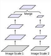
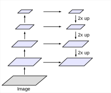
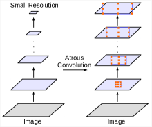
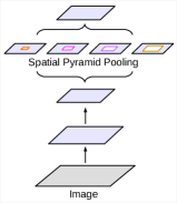
Another difficulty comes from the existence of objects at multiple scales. Several methods have been proposed to handle the problem and we mainly consider four categories in this work, as illustrated in Fig. 2. First, the DCNN is applied to an image pyramid to extract features for each scale input [22, 19, 69, 55, 12, 11] where objects at different scales become prominent at different feature maps. Second, the encoder-decoder structure [3, 71, 25, 54, 70, 68, 39] exploits multi-scale features from the encoder part and recovers the spatial resolution from the decoder part. Third, extra modules are cascaded on top of the original network for capturing long range information. In particular, DenseCRF [45] is employed to encode pixel-level pairwise similarities [10, 96, 55, 73], while [59, 90] develop several extra convolutional layers in cascade to gradually capture long range context. Fourth, spatial pyramid pooling [11, 95] probes an incoming feature map with filters or pooling operations at multiple rates and multiple effective field-of-views, thus capturing objects at multiple scales.
 |
 |
 |
 |
| (a) Image Pyramid | (b) Encoder-Decoder | (c) Deeper w. Atrous Convolution | (d) Spatial Pyramid Pooling |
In this work, we revisit applying atrous convolution, which allows us to effectively enlarge the field of view of filters to incorporate multi-scale context, in the framework of both cascaded modules and spatial pyramid pooling. In particular, our proposed module consists of atrous convolution with various rates and batch normalization layers which we found important to be trained as well. We experiment with laying out the modules in cascade or in parallel (specifically, Atrous Spatial Pyramid Pooling (ASPP) method [11]). We discuss an important practical issue when applying a atrous convolution with an extremely large rate, which fails to capture long range information due to image boundary effects, effectively simply degenerating to convolution, and propose to incorporate image-level features into the ASPP module. Furthermore, we elaborate on implementation details and share experience on training the proposed models, including a simple yet effective bootstrapping method for handling rare and finely annotated objects. In the end, our proposed model, ‘DeepLabv3’ improves over our previous works [10, 11] and attains performance of 85.7% on the PASCAL VOC 2012 test set without DenseCRF post-processing.
2 Related Work
It has been shown that global features or contextual interactions [33, 76, 43, 48, 27, 89] are beneficial in correctly classifying pixels for semantic segmentation. In this work, we discuss four types of Fully Convolutional Networks (FCNs) [74, 60] (see Fig. 2 for illustration) that exploit context information for semantic segmentation [30, 15, 62, 9, 96, 55, 65, 73, 87].
Image pyramid: The same model, typically with shared weights, is applied to multi-scale inputs. Feature responses from the small scale inputs encode the long-range context, while the large scale inputs preserve the small object details. Typical examples include Farabet et al. [22] who transform the input image through a Laplacian pyramid, feed each scale input to a DCNN and merge the feature maps from all the scales. [19, 69] apply multi-scale inputs sequentially from coarse-to-fine, while [55, 12, 11] directly resize the input for several scales and fuse the features from all the scales. The main drawback of this type of models is that it does not scale well for larger/deeper DCNNs (e.g., networks like [32, 91, 86]) due to limited GPU memory and thus it is usually applied during the inference stage [16].
Encoder-decoder: This model consists of two parts: (a) the encoder where the spatial dimension of feature maps is gradually reduced and thus longer range information is more easily captured in the deeper encoder output, and (b) the decoder where object details and spatial dimension are gradually recovered. For example, [60, 64] employ deconvolution [92] to learn the upsampling of low resolution feature responses. SegNet [3] reuses the pooling indices from the encoder and learn extra convolutional layers to densify the feature responses, while U-Net [71] adds skip connections from the encoder features to the corresponding decoder activations, and [25] employs a Laplacian pyramid reconstruction network. More recently, RefineNet [54] and [70, 68, 39] have demonstrated the effectiveness of models based on encoder-decoder structure on several semantic segmentation benchmarks. This type of model is also explored in the context of object detection [56, 77].
Context module: This model contains extra modules laid out in cascade to encode long-range context. One effective method is to incorporate DenseCRF [45] (with efficient high-dimensional filtering algorithms [2]) to DCNNs [10, 11]. Furthermore, [96, 55, 73] propose to jointly train both the CRF and DCNN components, while [59, 90] employ several extra convolutional layers on top of the belief maps of DCNNs (belief maps are the final DCNN feature maps that contain output channels equal to the number of predicted classes) to capture context information. Recently, [41] proposes to learn a general and sparse high-dimensional convolution (bilateral convolution), and [82, 8] combine Gaussian Conditional Random Fields and DCNNs for semantic segmentation.
Spatial pyramid pooling: This model employs spatial pyramid pooling [28, 49] to capture context at several ranges. The image-level features are exploited in ParseNet [58] for global context information. DeepLabv2 [11] proposes atrous spatial pyramid pooling (ASPP), where parallel atrous convolution layers with different rates capture multi-scale information. Recently, Pyramid Scene Parsing Net (PSP) [95] performs spatial pooling at several grid scales and demonstrates outstanding performance on several semantic segmentation benchmarks. There are other methods based on LSTM [35] to aggregate global context [53, 6, 88]. Spatial pyramid pooling has also been applied in object detection [31].
In this work, we mainly explore atrous convolution [36, 26, 74, 66, 10, 90, 11] as a context module and tool for spatial pyramid pooling. Our proposed framework is general in the sense that it could be applied to any network. To be concrete, we duplicate several copies of the original last block in ResNet [32] and arrange them in cascade, and also revisit the ASPP module [11] which contains several atrous convolutions in parallel. Note that our cascaded modules are applied directly on the feature maps instead of belief maps. For the proposed modules, we experimentally find it important to train with batch normalization [38]. To further capture global context, we propose to augment ASPP with image-level features, similar to [58, 95].
Atrous convolution: Models based on atrous convolution have been actively explored for semantic segmentation. For example, [85] experiments with the effect of modifying atrous rates for capturing long-range information, [84] adopts hybrid atrous rates within the last two blocks of ResNet, while [18] further proposes to learn the deformable convolution which samples the input features with learned offset, generalizing atrous convolution. To further improve the segmentation model accuracy, [83] exploits image captions, [40] utilizes video motion, and [44] incorporates depth information. Besides, atrous convolution has been applied to object detection by [66, 17, 37].
3 Methods
In this section, we review how atrous convolution is applied to extract dense features for semantic segmentation. We then discuss the proposed modules with atrous convolution modules employed in cascade or in parallel.
 |
| (a) Going deeper without atrous convolution. |
 |
| (b) Going deeper with atrous convolution. Atrous convolution with is applied after block3 when . |
3.1 Atrous Convolution for Dense Feature Extraction
Deep Convolutional Neural Networks (DCNNs) [50] deployed in fully convolutional fashion [74, 60] have shown to be effective for the task of semantic segmentation. However, the repeated combination of max-pooling and striding at consecutive layers of these networks significantly reduces the spatial resolution of the resulting feature maps, typically by a factor of 32 across each direction in recent DCNNs [47, 78, 32]. Deconvolutional layers (or transposed convolution) [92, 60, 64, 3, 71, 68] have been employed to recover the spatial resolution. Instead, we advocate the use of ‘atrous convolution’, originally developed for the efficient computation of the undecimated wavelet transform in the “algorithme à trous” scheme of [36] and used before in the DCNN context by [26, 74, 66].
Consider two-dimensional signals, for each location on the output and a filter , atrous convolution is applied over the input feature map :
| (1) |
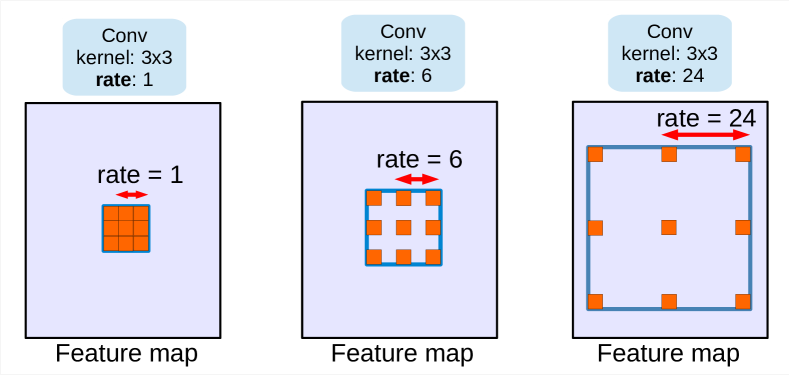
where the atrous rate r corresponds to the stride with which we sample the input signal, which is equivalent to convolving the input with upsampled filters produced by inserting zeros between two consecutive filter values along each spatial dimension (hence the name atrous convolution where the French word trous means holes in English). Standard convolution is a special case for rate , and atrous convolution allows us to adaptively modify filter’s field-of-view by changing the rate value. See Fig. 1 for illustration.
Atrous convolution also allows us to explicitly control how densely to compute feature responses in fully convolutional networks. Here, we denote by output_stride the ratio of input image spatial resolution to final output resolution. For the DCNNs [47, 78, 32] deployed for the task of image classification, the final feature responses (before fully connected layers or global pooling) is 32 times smaller than the input image dimension, and thus . If one would like to double the spatial density of computed feature responses in the DCNNs (i.e., ), the stride of last pooling or convolutional layer that decreases resolution is set to 1 to avoid signal decimation. Then, all subsequent convolutional layers are replaced with atrous convolutional layers having rate . This allows us to extract denser feature responses without requiring learning any extra parameters. Please refer to [11] for more details.
3.2 Going Deeper with Atrous Convolution
We first explore designing modules with atrous convolution laid out in cascade. To be concrete, we duplicate several copies of the last ResNet block, denoted as block4 in Fig. 3, and arrange them in cascade. There are three convolutions in those blocks, and the last convolution contains stride 2 except the one in last block, similar to original ResNet. The motivation behind this model is that the introduced striding makes it easy to capture long range information in the deeper blocks. For example, the whole image feature could be summarized in the last small resolution feature map, as illustrated in Fig. 3 (a). However, we discover that the consecutive striding is harmful for semantic segmentation (see Tab. 1 in Sec. 4) since detail information is decimated, and thus we apply atrous convolution with rates determined by the desired output_stride value, as shown in Fig. 3 (b) where .
In this proposed model, we experiment with cascaded ResNet blocks up to block7 (i.e., extra block5, block6, block7 as replicas of block4), which has if no atrous convolution is applied.
3.2.1 Multi-grid Method
Motivated by multi-grid methods which employ a hierarchy of grids of different sizes [4, 81, 5, 67] and following [84, 18], we adopt different atrous rates within block4 to block7 in the proposed model. In particular, we define as the unit rates for the three convolutional layers within block4 to block7. The final atrous rate for the convolutional layer is equal to the multiplication of the unit rate and the corresponding rate. For example, when and , the three convolutions will have in the block4, respectively.
3.3 Atrous Spatial Pyramid Pooling
We revisit the Atrous Spatial Pyramid Pooling proposed in [11], where four parallel atrous convolutions with different atrous rates are applied on top of the feature map. ASPP is inspired by the success of spatial pyramid pooling [28, 49, 31] which showed that it is effective to resample features at different scales for accurately and efficiently classifying regions of an arbitrary scale. Different from [11], we include batch normalization within ASPP.
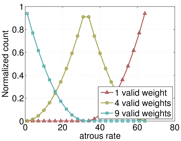
ASPP with different atrous rates effectively captures multi-scale information. However, we discover that as the sampling rate becomes larger, the number of valid filter weights (i.e., the weights that are applied to the valid feature region, instead of padded zeros) becomes smaller. This effect is illustrated in Fig. 4 when applying a filter to a feature map with different atrous rates. In the extreme case where the rate value is close to the feature map size, the filter, instead of capturing the whole image context, degenerates to a simple filter since only the center filter weight is effective.
To overcome this problem and incorporate global context information to the model, we adopt image-level features, similar to [58, 95]. Specifically, we apply global average pooling on the last feature map of the model, feed the resulting image-level features to a convolution with 256 filters (and batch normalization [38]), and then bilinearly upsample the feature to the desired spatial dimension. In the end, our improved ASPP consists of (a) one convolution and three convolutions with when (all with 256 filters and batch normalization), and (b) the image-level features, as shown in Fig. 5. Note that the rates are doubled when . The resulting features from all the branches are then concatenated and pass through another convolution (also with 256 filters and batch normalization) before the final convolution which generates the final logits.
 |
 |
4 Experimental Evaluation
We adapt the ImageNet-pretrained [72] ResNet [32] to the semantic segmentation by applying atrous convolution to extract dense features. Recall that output_stride is defined as the ratio of input image spatial resolution to final output resolution. For example, when , the last two blocks (block3 and block4 in our notation) in the original ResNet contains atrous convolution with and respectively. Our implementation is built on TensorFlow [1].
We evaluate the proposed models on the PASCAL VOC 2012 semantic segmentation benchmark [20] which contains 20 foreground object classes and one background class. The original dataset contains (train), (val), and (test) pixel-level labeled images for training, validation, and testing, respectively. The dataset is augmented by the extra annotations provided by [29], resulting in (trainaug) training images. The performance is measured in terms of pixel intersection-over-union (IOU) averaged across the 21 classes.
4.1 Training Protocol
In this subsection, we discuss details of our training protocol.
Learning rate policy: Similar to [58, 11], we employ a “poly” learning rate policy where the initial learning rate is multiplied by with .
Crop size: Following the original training protocol [10, 11], patches are cropped from the image during training. For atrous convolution with large rates to be effective, large crop size is required; otherwise, the filter weights with large atrous rate are mostly applied to the padded zero region. We thus employ crop size to be 513 during both training and test on PASCAL VOC 2012 dataset.
Batch normalization: Our added modules on top of ResNet all include batch normalization parameters [38], which we found important to be trained as well. Since large batch size is required to train batch normalization parameters, we employ and compute the batch normalization statistics with a batch size of 16. The batch normalization parameters are trained with decay = 0.9997. After training on the trainaug set with 30K iterations and initial learning rate = 0.007, we then freeze batch normalization parameters, employ , and train on the official PASCAL VOC 2012 trainval set for another 30K iterations and smaller base learning rate = 0.001. Note that atrous convolution allows us to control output_stride value at different training stages without requiring learning extra model parameters. Also note that training with is several times faster than since the intermediate feature maps are spatially four times smaller, but at a sacrifice of accuracy since provides coarser feature maps.
Upsampling logits: In our previous works [10, 11], the target groundtruths are downsampled by 8 during training when . We find it important to keep the groundtruths intact and instead upsample the final logits, since downsampling the groundtruths removes the fine annotations resulting in no back-propagation of details.
Data augmentation: We apply data augmentation by randomly scaling the input images (from 0.5 to 2.0) and randomly left-right flipping during training.
4.2 Going Deeper with Atrous Convolution
We first experiment with building more blocks with atrous convolution in cascade.
ResNet-50: In Tab. 1, we experiment with the effect of output_stride when employing ResNet-50 with block7 (i.e., extra block5, block6, and block7). As shown in the table, in the case of (i.e., no atrous convolution at all), the performance is much worse than the others due to the severe signal decimation. When output_stride gets larger and apply atrous convolution correspondingly, the performance improves from 20.29% to 75.18%, showing that atrous convolution is essential when building more blocks cascadedly for semantic segmentation.
| output_stride | 8 | 16 | 32 | 64 | 128 | 256 |
|---|---|---|---|---|---|---|
| mIOU | 75.18 | 73.88 | 70.06 | 59.99 | 42.34 | 20.29 |
| Network | block4 | block5 | block6 | block7 |
|---|---|---|---|---|
| ResNet-50 | 64.81 | 72.14 | 74.29 | 73.88 |
| ResNet-101 | 68.39 | 73.21 | 75.34 | 75.76 |
| Multi-Grid | block4 | block5 | block6 | block7 |
|---|---|---|---|---|
| (1, 1, 1) | 68.39 | 73.21 | 75.34 | 75.76 |
| (1, 2, 1) | 70.23 | 75.67 | 76.09 | 76.66 |
| (1, 2, 3) | 73.14 | 75.78 | 75.96 | 76.11 |
| (1, 2, 4) | 73.45 | 75.74 | 75.85 | 76.02 |
| (2, 2, 2) | 71.45 | 74.30 | 74.70 | 74.62 |
ResNet-50 vs. ResNet-101: We replace ResNet-50 with deeper network ResNet-101 and change the number of cascaded blocks. As shown in Tab. 2, the performance improves as more blocks are added, but the margin of improvement becomes smaller. Noticeably, employing block7 to ResNet-50 decreases slightly the performance while it still improves the performance for ResNet-101.
Multi-grid: We apply the multi-grid method to ResNet-101 with several cascadedly added blocks in Tab. 3. The unit rates, , are applied to block4 and all the other added blocks. As shown in the table, we observe that (a) applying multi-grid method is generally better than the vanilla version where , (b) simply doubling the unit rates (i.e., ) is not effective, and (c) going deeper with multi-grid improves the performance. Our best model is the case where block7 and are employed.
Inference strategy on val set: The proposed model is trained with , and then during inference we apply to get more detailed feature map. As shown in Tab. 4, interestingly, when evaluating our best cascaded model with , the performance improves over evaluating with by . The performance is further improved by performing inference on multi-scale inputs (with ) and also left-right flipped images. In particular, we compute as the final result the average probabilities from each scale and flipped images.
| Method | OS=16 | OS=8 | MS | Flip | mIOU |
|---|---|---|---|---|---|
| block7 + | ✓ | 76.66 | |||
| MG(1, 2, 1) | ✓ | 78.05 | |||
| ✓ | ✓ | 78.93 | |||
| ✓ | ✓ | ✓ | 79.35 |
4.3 Atrous Spatial Pyramid Pooling
We then experiment with the Atrous Spatial Pyramid Pooling (ASPP) module with the main differences from [11] being that batch normalization parameters [38] are fine-tuned and image-level features are included.
| Multi-Grid | ASPP | Image | ||||
|---|---|---|---|---|---|---|
| (1, 1, 1) | (1, 2, 1) | (1, 2, 4) | (6, 12, 18) | (6, 12, 18, 24) | Pooling | mIOU |
| ✓ | ✓ | 75.36 | ||||
| ✓ | ✓ | 75.93 | ||||
| ✓ | ✓ | 76.58 | ||||
| ✓ | ✓ | 76.46 | ||||
| ✓ | ✓ | ✓ | 77.21 | |||
| Method | OS=16 | OS=8 | MS | Flip | COCO | mIOU |
|---|---|---|---|---|---|---|
| MG(1, 2, 4) + | ✓ | 77.21 | ||||
| ASPP(6, 12, 18) + | ✓ | 78.51 | ||||
| Image Pooling | ✓ | ✓ | 79.45 | |||
| ✓ | ✓ | ✓ | 79.77 | |||
| ✓ | ✓ | ✓ | ✓ | 82.70 |
ASPP: In Tab. 5, we experiment with the effect of incorporating multi-grid in block4 and image-level features to the improved ASPP module. We first fix (i.e., employ for the three parallel convolution branches), and vary the multi-grid value. Employing is better than , while further improvement is attained by adopting in the context of (cf., the ‘block4’ column in Tab. 3). If we additionally employ another parallel branch with for longer range context, the performance drops slightly by 0.12%. On the other hand, augmenting the ASPP module with image-level feature is effective, reaching the final performance of 77.21%.
Inference strategy on val set: Similarly, we apply during inference once the model is trained. As shown in Tab. 6, employing brings 1.3% improvement over using , adopting multi-scale inputs and adding left-right flipped images further improve the performance by 0.94% and 0.32%, respectively. The best model with ASPP attains the performance of 79.77%, better than the best model with cascaded atrous convolution modules (79.35%), and thus is selected as our final model for test set evaluation.
Comparison with DeepLabv2: Both our best cascaded model (in Tab. 4) and ASPP model (in Tab. 6) (in both cases without DenseCRF post-processing or MS-COCO pre-training) already outperform DeepLabv2 (77.69% with DenseCRF and pretrained on MS-COCO in Tab. 4 of [11]) on the PASCAL VOC 2012 val set. The improvement mainly comes from including and fine-tuning batch normalization parameters [38] in the proposed models and having a better way to encode multi-scale context.
Appendix: We show more experimental results, such as the effect of hyper parameters and Cityscapes [14] results, in the appendix.
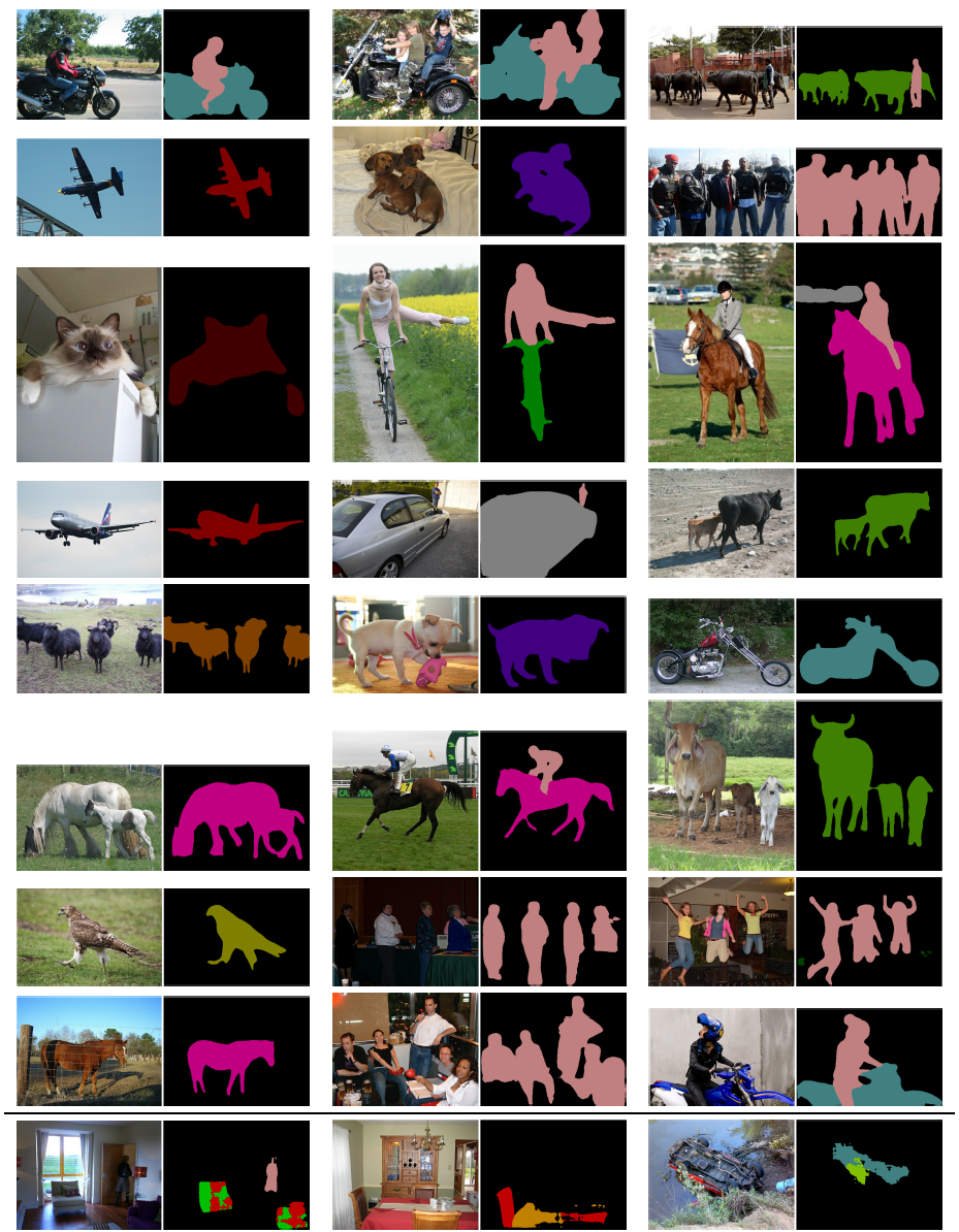
Qualitative results: We provide qualitative visual results of our best ASPP model in Fig. 6. As shown in the figure, our model is able to segment objects very well without any DenseCRF post-processing.
Failure mode: As shown in the bottom row of Fig. 6, our model has difficulty in segmenting (a) sofa vs. chair, (b) dining table and chair, and (c) rare view of objects.
 |
Pretrained on COCO: For comparison with other state-of-art models, we further pretrain our best ASPP model on MS-COCO dataset [57]. From the MS-COCO trainval_minus_minival set, we only select the images that have annotation regions larger than 1000 pixels and contain the classes defined in PASCAL VOC 2012, resulting in about 60K images for training. Besides, the MS-COCO classes not defined in PASCAL VOC 2012 are all treated as background class. After pretraining on MS-COCO dataset, our proposed model attains performance of 82.7% on val set when using , multi-scale inputs and adding left-right flipped images during inference. We adopt smaller initial learning rate = 0.0001 and same training protocol as in Sec. 4.1 when fine-tuning on PASCAL VOC 2012 dataset.
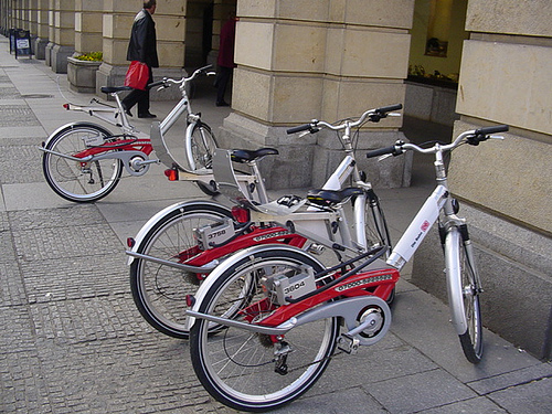
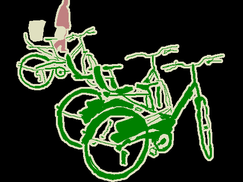
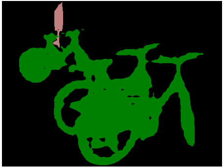
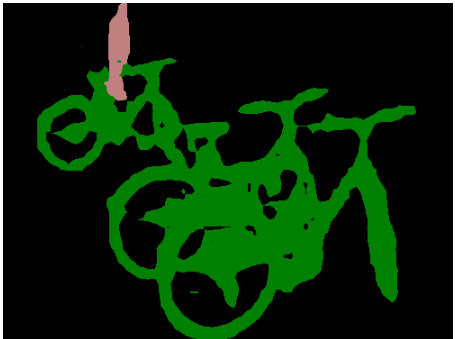
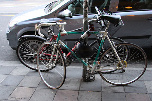
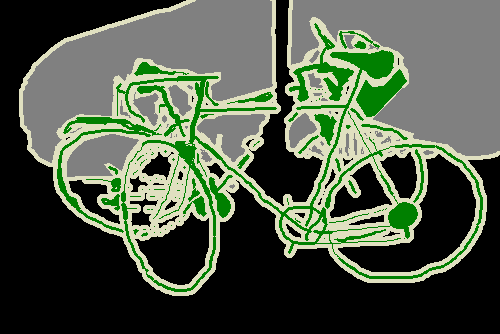
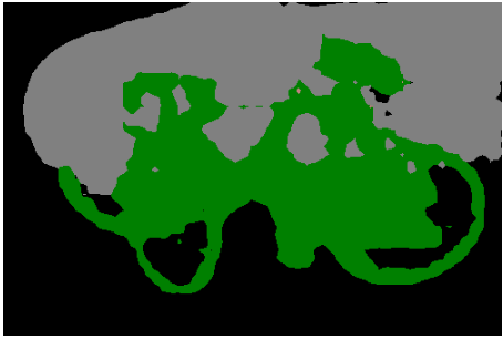
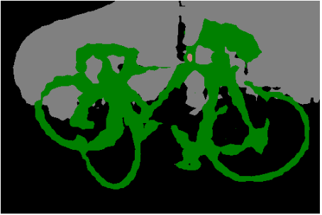
Test set result and an effective bootstrapping method: We notice that PASCAL VOC 2012 dataset provides higher quality of annotations than the augmented dataset [29], especially for the bicycle class. We thus further fine-tune our model on the official PASCAL VOC 2012 trainval set before evaluating on the test set. Specifically, our model is trained with (so that annotation details are kept) and the batch normalization parameters are frozen (see Sec. 4.1 for details). Besides, instead of performing pixel hard example mining as [85, 70], we resort to bootstrapping on hard images. In particular, we duplicate the images that contain hard classes (namely bicycle, chair, table, pottedplant, and sofa) in the training set. As shown in Fig. 7, the simple bootstrapping method is effective for segmenting the bicycle class. In the end, our ‘DeepLabv3’ achieves the performance of 85.7% on the test set without any DenseCRF post-processing, as shown in Tab. 7.
 |
 |
 |
 |
 |
 |
 |
 |
| (a) Image | (b) G.T. | (c) w/o bootstrapping | (d) w/ bootstrapping |
| Method | mIOU |
|---|---|
| Adelaide_VeryDeep_FCN_VOC [85] | 79.1 |
| LRR_4x_ResNet-CRF [25] | 79.3 |
| DeepLabv2-CRF [11] | 79.7 |
| CentraleSupelec Deep G-CRF [8] | 80.2 |
| HikSeg_COCO [80] | 81.4 |
| SegModel [75] | 81.8 |
| Deep Layer Cascade (LC) [52] | 82.7 |
| TuSimple [84] | 83.1 |
| Large_Kernel_Matters [68] | 83.6 |
| Multipath-RefineNet [54] | 84.2 |
| ResNet-38_MS_COCO [86] | 84.9 |
| PSPNet [95] | 85.4 |
| IDW-CNN [83] | 86.3 |
| CASIA_IVA_SDN [23] | 86.6 |
| DIS [61] | 86.8 |
| DeepLabv3 | 85.7 |
| DeepLabv3-JFT | 86.9 |
5 Conclusion
Our proposed model “DeepLabv3” employs atrous convolution with upsampled filters to extract dense feature maps and to capture long range context. Specifically, to encode multi-scale information, our proposed cascaded module gradually doubles the atrous rates while our proposed atrous spatial pyramid pooling module augmented with image-level features probes the features with filters at multiple sampling rates and effective field-of-views. Our experimental results show that the proposed model significantly improves over previous DeepLab versions and achieves comparable performance with other state-of-art models on the PASCAL VOC 2012 semantic image segmentation benchmark.
Acknowledgments
We would like to acknowledge valuable discussions with Zbigniew Wojna, the help from Chen Sun and Andrew Howard, and the support from Google Mobile Vision team.
Appendix A Effect of hyper-parameters
In this section, we follow the same training protocol as in the main paper and experiment with the effect of some hyper-parameters.
New training protocol: As mentioned in the main paper, we change the training protocol in [10, 11] with three main differences: (1) larger crop size, (2) upsampling logits during training, and (3) fine-tuning batch normalization. Here, we quantitatively measure the effect of the changes. As shown in Tab. 8, DeepLabv3 attains the performance of 77.21% on the PASCAL VOC 2012 val set [20] when adopting the new training protocol setting as in the main paper. When training DeepLabv3 without fine-tuning the batch normalization, the performance drops to 75.95%. If we do not upsample the logits during training (and instead downsample the groundtruths), the performance decreases to 76.01%. Furthermore, if we employ smaller value of crop size (i.e., 321 as in [10, 11]), the performance significantly decreases to 67.22%, demonstrating that boundary effect resulted from small crop size hurts the performance of DeepLabv3 which employs large atrous rates in the Atrous Spatial Pyramid Pooling (ASPP) module.
Varying batch size: Since it is important to train DeepLabv3 with fine-tuning the batch normalization, we further experiment with the effect of different batch sizes. As shown in Tab. 9, employing small batch size is inefficient to train the model, while using larger batch size leads to better performance.
Output stride: The value of output_stride determines the output feature map resolution and in turn affects the largest batch size we could use during training. In Tab. 10, we quantitatively measure the effect of employing different output_stride values during both training and evaluation on the PASCAL VOC 2012 val set. We first fix the evaluation , vary the training output_stride and fit the largest possible batch size for all the settings (we are able to fit batch size 6, 16, and 24 for training output_stride equal to 8, 16, and 32, respectively). As shown in the top rows of Tab. 10, employing training only attains the performance of 74.45% because we could not fit large batch size in this setting which degrades the performance while fine-tuning the batch normalization parameters. When employing training , we could fit large batch size but we lose feature map details. On the other hand, employing training strikes the best trade-off and leads to the best performance. In the bottom rows of Tab. 10, we increase the evaluation . All settings improve the performance except the one where training . We hypothesize that we lose too much feature map details during training, and thus the model could not recover the details even when employing during evaluation.
| Crop Size | UL | BN | mIOU |
|---|---|---|---|
| 513 | ✓ | ✓ | 77.21 |
| 513 | ✓ | 75.95 | |
| 513 | ✓ | 76.01 | |
| 321 | ✓ | 67.22 |
| batch size | mIOU |
|---|---|
| 4 | 64.43 |
| 8 | 75.76 |
| 12 | 76.49 |
| 16 | 77.21 |
| train output_stride | eval output_stride | mIOU |
| 8 | 16 | 74.45 |
| 16 | 16 | 77.21 |
| 32 | 16 | 75.90 |
| 8 | 8 | 75.62 |
| 16 | 8 | 78.51 |
| 32 | 8 | 75.75 |
Appendix B Asynchronous training
In this section, we experiment DeepLabv3 with TensorFlow asynchronous training [1]. We measure the effect of training the model with multiple replicas on PASCAL VOC 2012 semantic segmentation dataset. Our baseline employs simply one replica and requires training time 3.65 days with a K80 GPU. As shown in Tab. 11, we found that the performance of using multiple replicas does not drop compared to the baseline. However, training time with 32 replicas is significantly reduced to 2.74 hours.
| num replicas | mIOU | relative training time |
|---|---|---|
| 1 | 77.21 | 1.00x |
| 2 | 77.15 | 0.50x |
| 4 | 76.79 | 0.25x |
| 8 | 77.02 | 0.13x |
| 16 | 77.18 | 0.06x |
| 32 | 76.69 | 0.03x |
Appendix C DeepLabv3 on Cityscapes dataset
Cityscapes [14] is a large-scale dataset containing high quality pixel-level annotations of 5000 images (2975, 500, and 1525 for the training, validation, and test sets respectively) and about 20000 coarsely annotated images. Following the evaluation protocol [14], 19 semantic labels are used for evaluation without considering the void label.
We first evaluate the proposed DeepLabv3 model on the validation set when training with only 2975 images (i.e., train_fine set). We adopt the same training protocol as before except that we employ 90K training iterations, crop size equal to 769, and running inference on the whole image, instead of on the overlapped regions as in [11]. As shown in Tab. 12, DeepLabv3 attains the performance of 77.23% when evaluating at . Evaluating the model at improves the performance to 77.82%. When we employ multi-scale inputs (we could fit on a K40 GPU) and add left-right flipped inputs, the model achieves 79.30%.
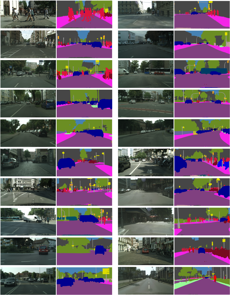
In order to compete with other state-of-art models, we further train DeepLabv3 on the trainval_coarse set (i.e., the 3475 finely annotated images and the extra 20000 coarsely annotated images). We adopt more scales and finer output_stride during inference. In particular, we perform inference with and evaluation with CPUs, which contributes extra 0.8% and 0.1% respectively on the validation set compared to using only three scales and . In the end, as shown in Tab. 13, our proposed DeepLabv3 achieves the performance of 81.3% on the test set. Some results on val set are visualized in Fig. 8.
| OS=16 | OS=8 | MS | Flip | mIOU |
|---|---|---|---|---|
| ✓ | 77.23 | |||
| ✓ | 77.82 | |||
| ✓ | ✓ | 79.06 | ||
| ✓ | ✓ | ✓ | 79.30 |
| Method | Coarse | mIOU |
|---|---|---|
| DeepLabv2-CRF [11] | 70.4 | |
| Deep Layer Cascade [52] | 71.1 | |
| ML-CRNN [21] | 71.2 | |
| Adelaide_context [55] | 71.6 | |
| FRRN [70] | 71.8 | |
| LRR-4x [25] | ✓ | 71.8 |
| RefineNet [54] | 73.6 | |
| FoveaNet [51] | 74.1 | |
| Ladder DenseNet [46] | 74.3 | |
| PEARL [42] | 75.4 | |
| Global-Local-Refinement [93] | 77.3 | |
| SAC_multiple [94] | 78.1 | |
| SegModel [75] | ✓ | 79.2 |
| TuSimple_Coarse [84] | ✓ | 80.1 |
| Netwarp [24] | ✓ | 80.5 |
| ResNet-38 [86] | ✓ | 80.6 |
| PSPNet [95] | ✓ | 81.2 |
| DeepLabv3 | ✓ | 81.3 |
 |
References
- [1] M. Abadi, A. Agarwal, et al. Tensorflow: Large-scale machine learning on heterogeneous distributed systems. arXiv:1603.04467, 2016.
- [2] A. Adams, J. Baek, and M. A. Davis. Fast high-dimensional filtering using the permutohedral lattice. In Eurographics, 2010.
- [3] V. Badrinarayanan, A. Kendall, and R. Cipolla. Segnet: A deep convolutional encoder-decoder architecture for image segmentation. arXiv:1511.00561, 2015.
- [4] A. Brandt. Multi-level adaptive solutions to boundary-value problems. Mathematics of computation, 31(138):333–390, 1977.
- [5] W. L. Briggs, V. E. Henson, and S. F. McCormick. A multigrid tutorial. SIAM, 2000.
- [6] W. Byeon, T. M. Breuel, F. Raue, and M. Liwicki. Scene labeling with lstm recurrent neural networks. In CVPR, 2015.
- [7] H. Caesar, J. Uijlings, and V. Ferrari. COCO-Stuff: Thing and stuff classes in context. arXiv:1612.03716, 2016.
- [8] S. Chandra and I. Kokkinos. Fast, exact and multi-scale inference for semantic image segmentation with deep Gaussian CRFs. arXiv:1603.08358, 2016.
- [9] L.-C. Chen, J. T. Barron, G. Papandreou, K. Murphy, and A. L. Yuille. Semantic image segmentation with task-specific edge detection using cnns and a discriminatively trained domain transform. In CVPR, 2016.
- [10] L.-C. Chen, G. Papandreou, I. Kokkinos, K. Murphy, and A. L. Yuille. Semantic image segmentation with deep convolutional nets and fully connected crfs. In ICLR, 2015.
- [11] L.-C. Chen, G. Papandreou, I. Kokkinos, K. Murphy, and A. L. Yuille. Deeplab: Semantic image segmentation with deep convolutional nets, atrous convolution, and fully connected crfs. arXiv:1606.00915, 2016.
- [12] L.-C. Chen, Y. Yang, J. Wang, W. Xu, and A. L. Yuille. Attention to scale: Scale-aware semantic image segmentation. In CVPR, 2016.
- [13] F. Chollet. Xception: Deep learning with depthwise separable convolutions. arXiv:1610.02357, 2016.
- [14] M. Cordts, M. Omran, S. Ramos, T. Rehfeld, M. Enzweiler, R. Benenson, U. Franke, S. Roth, and B. Schiele. The cityscapes dataset for semantic urban scene understanding. In CVPR, 2016.
- [15] J. Dai, K. He, and J. Sun. Convolutional feature masking for joint object and stuff segmentation. arXiv:1412.1283, 2014.
- [16] J. Dai, K. He, and J. Sun. Boxsup: Exploiting bounding boxes to supervise convolutional networks for semantic segmentation. In ICCV, 2015.
- [17] J. Dai, Y. Li, K. He, and J. Sun. R-fcn: Object detection via region-based fully convolutional networks. arXiv:1605.06409, 2016.
- [18] J. Dai, H. Qi, Y. Xiong, Y. Li, G. Zhang, H. Hu, and Y. Wei. Deformable convolutional networks. arXiv:1703.06211, 2017.
- [19] D. Eigen and R. Fergus. Predicting depth, surface normals and semantic labels with a common multi-scale convolutional architecture. arXiv:1411.4734, 2014.
- [20] M. Everingham, S. M. A. Eslami, L. V. Gool, C. K. I. Williams, J. Winn, and A. Zisserma. The pascal visual object classes challenge – a retrospective. IJCV, 2014.
- [21] H. Fan, X. Mei, D. Prokhorov, and H. Ling. Multi-level contextual rnns with attention model for scene labeling. arXiv:1607.02537, 2016.
- [22] C. Farabet, C. Couprie, L. Najman, and Y. LeCun. Learning hierarchical features for scene labeling. PAMI, 2013.
- [23] J. Fu, J. Liu, Y. Wang, and H. Lu. Stacked deconvolutional network for semantic segmentation. arXiv:1708.04943, 2017.
- [24] R. Gadde, V. Jampani, and P. V. Gehler. Semantic video cnns through representation warping. In ICCV, 2017.
- [25] G. Ghiasi and C. C. Fowlkes. Laplacian reconstruction and refinement for semantic segmentation. arXiv:1605.02264, 2016.
- [26] A. Giusti, D. Ciresan, J. Masci, L. Gambardella, and J. Schmidhuber. Fast image scanning with deep max-pooling convolutional neural networks. In ICIP, 2013.
- [27] S. Gould, R. Fulton, and D. Koller. Decomposing a scene into geometric and semantically consistent regions. In ICCV. IEEE, 2009.
- [28] K. Grauman and T. Darrell. The pyramid match kernel: Discriminative classification with sets of image features. In ICCV, 2005.
- [29] B. Hariharan, P. Arbeláez, L. Bourdev, S. Maji, and J. Malik. Semantic contours from inverse detectors. In ICCV, 2011.
- [30] B. Hariharan, P. Arbeláez, R. Girshick, and J. Malik. Hypercolumns for object segmentation and fine-grained localization. In CVPR, 2015.
- [31] K. He, X. Zhang, S. Ren, and J. Sun. Spatial pyramid pooling in deep convolutional networks for visual recognition. In ECCV, 2014.
- [32] K. He, X. Zhang, S. Ren, and J. Sun. Deep residual learning for image recognition. arXiv:1512.03385, 2015.
- [33] X. He, R. S. Zemel, and M. Carreira-Perpindn. Multiscale conditional random fields for image labeling. In CVPR, 2004.
- [34] G. Hinton, O. Vinyals, and J. Dean. Distilling the knowledge in a neural network. In NIPS, 2014.
- [35] S. Hochreiter and J. Schmidhuber. Long short-term memory. Neural computation, 9(8):1735–1780, 1997.
- [36] M. Holschneider, R. Kronland-Martinet, J. Morlet, and P. Tchamitchian. A real-time algorithm for signal analysis with the help of the wavelet transform. In Wavelets: Time-Frequency Methods and Phase Space, pages 289–297. 1989.
- [37] J. Huang, V. Rathod, C. Sun, M. Zhu, A. Korattikara, A. Fathi, I. Fischer, Z. Wojna, Y. Song, S. Guadarrama, and K. Murphy. Speed/accuracy trade-offs for modern convolutional object detectors. In CVPR, 2017.
- [38] S. Ioffe and C. Szegedy. Batch normalization: Accelerating deep network training by reducing internal covariate shift. arXiv:1502.03167, 2015.
- [39] M. A. Islam, M. Rochan, N. D. Bruce, and Y. Wang. Gated feedback refinement network for dense image labeling. In CVPR, 2017.
- [40] S. D. Jain, B. Xiong, and K. Grauman. Fusionseg: Learning to combine motion and appearance for fully automatic segmention of generic objects in videos. In CVPR, 2017.
- [41] V. Jampani, M. Kiefel, and P. V. Gehler. Learning sparse high dimensional filters: Image filtering, dense crfs and bilateral neural networks. In CVPR, 2016.
- [42] X. Jin, X. Li, H. Xiao, X. Shen, Z. Lin, J. Yang, Y. Chen, J. Dong, L. Liu, Z. Jie, J. Feng, and S. Yan. Video scene parsing with predictive feature learning. In ICCV, 2017.
- [43] P. Kohli, P. H. Torr, et al. Robust higher order potentials for enforcing label consistency. IJCV, 82(3):302–324, 2009.
- [44] S. Kong and C. Fowlkes. Recurrent scene parsing with perspective understanding in the loop. arXiv:1705.07238, 2017.
- [45] P. Krähenbühl and V. Koltun. Efficient inference in fully connected crfs with gaussian edge potentials. In NIPS, 2011.
- [46] I. Krešo, S. Šegvić, and J. Krapac. Ladder-style densenets for semantic segmentation of large natural images. In ICCV CVRSUAD workshop, 2017.
- [47] A. Krizhevsky, I. Sutskever, and G. E. Hinton. Imagenet classification with deep convolutional neural networks. In NIPS, 2012.
- [48] L. Ladicky, C. Russell, P. Kohli, and P. H. Torr. Associative hierarchical crfs for object class image segmentation. In ICCV, 2009.
- [49] S. Lazebnik, C. Schmid, and J. Ponce. Beyond bags of features: Spatial pyramid matching for recognizing natural scene categories. In CVPR, 2006.
- [50] Y. LeCun, B. Boser, J. S. Denker, D. Henderson, R. E. Howard, W. Hubbard, and L. D. Jackel. Backpropagation applied to handwritten zip code recognition. Neural computation, 1(4):541–551, 1989.
- [51] X. Li, Z. Jie, W. Wang, C. Liu, J. Yang, X. Shen, Z. Lin, Q. Chen, S. Yan, and J. Feng. Foveanet: Perspective-aware urban scene parsing. arXiv:1708.02421, 2017.
- [52] X. Li, Z. Liu, P. Luo, C. C. Loy, and X. Tang. Not all pixels are equal: Difficulty-aware semantic segmentation via deep layer cascade. arXiv:1704.01344, 2017.
- [53] X. Liang, X. Shen, D. Xiang, J. Feng, L. Lin, and S. Yan. Semantic object parsing with local-global long short-term memory. arXiv:1511.04510, 2015.
- [54] G. Lin, A. Milan, C. Shen, and I. Reid. Refinenet: Multi-path refinement networks with identity mappings for high-resolution semantic segmentation. arXiv:1611.06612, 2016.
- [55] G. Lin, C. Shen, I. Reid, et al. Efficient piecewise training of deep structured models for semantic segmentation. arXiv:1504.01013, 2015.
- [56] T.-Y. Lin, P. Dollár, R. Girshick, K. He, B. Hariharan, and S. Belongie. Feature pyramid networks for object detection. arXiv:1612.03144, 2016.
- [57] T.-Y. Lin, M. Maire, S. Belongie, J. Hays, P. Perona, D. Ramanan, P. Dollár, and C. L. Zitnick. Microsoft COCO: Common objects in context. In ECCV, 2014.
- [58] W. Liu, A. Rabinovich, and A. C. Berg. Parsenet: Looking wider to see better. arXiv:1506.04579, 2015.
- [59] Z. Liu, X. Li, P. Luo, C. C. Loy, and X. Tang. Semantic image segmentation via deep parsing network. In ICCV, 2015.
- [60] J. Long, E. Shelhamer, and T. Darrell. Fully convolutional networks for semantic segmentation. In CVPR, 2015.
- [61] P. Luo, G. Wang, L. Lin, and X. Wang. Deep dual learning for semantic image segmentation. In ICCV, 2017.
- [62] M. Mostajabi, P. Yadollahpour, and G. Shakhnarovich. Feedforward semantic segmentation with zoom-out features. In CVPR, 2015.
- [63] R. Mottaghi, X. Chen, X. Liu, N.-G. Cho, S.-W. Lee, S. Fidler, R. Urtasun, and A. Yuille. The role of context for object detection and semantic segmentation in the wild. In CVPR, 2014.
- [64] H. Noh, S. Hong, and B. Han. Learning deconvolution network for semantic segmentation. In ICCV, 2015.
- [65] G. Papandreou, L.-C. Chen, K. Murphy, and A. L. Yuille. Weakly- and semi-supervised learning of a dcnn for semantic image segmentation. In ICCV, 2015.
- [66] G. Papandreou, I. Kokkinos, and P.-A. Savalle. Modeling local and global deformations in deep learning: Epitomic convolution, multiple instance learning, and sliding window detection. In CVPR, 2015.
- [67] G. Papandreou and P. Maragos. Multigrid geometric active contour models. TIP, 16(1):229–240, 2007.
- [68] C. Peng, X. Zhang, G. Yu, G. Luo, and J. Sun. Large kernel matters–improve semantic segmentation by global convolutional network. arXiv:1703.02719, 2017.
- [69] P. Pinheiro and R. Collobert. Recurrent convolutional neural networks for scene labeling. In ICML, 2014.
- [70] T. Pohlen, A. Hermans, M. Mathias, and B. Leibe. Full-resolution residual networks for semantic segmentation in street scenes. arXiv:1611.08323, 2016.
- [71] O. Ronneberger, P. Fischer, and T. Brox. U-net: Convolutional networks for biomedical image segmentation. In MICCAI, 2015.
- [72] O. Russakovsky, J. Deng, H. Su, J. Krause, S. Satheesh, S. Ma, Z. Huang, A. Karpathy, A. Khosla, M. Bernstein, A. C. Berg, and L. Fei-Fei. ImageNet Large Scale Visual Recognition Challenge. IJCV, 2015.
- [73] A. G. Schwing and R. Urtasun. Fully connected deep structured networks. arXiv:1503.02351, 2015.
- [74] P. Sermanet, D. Eigen, X. Zhang, M. Mathieu, R. Fergus, and Y. LeCun. Overfeat: Integrated recognition, localization and detection using convolutional networks. arXiv:1312.6229, 2013.
- [75] F. Shen, R. Gan, S. Yan, and G. Zeng. Semantic segmentation via structured patch prediction, context crf and guidance crf. In CVPR, 2017.
- [76] J. Shotton, J. Winn, C. Rother, and A. Criminisi. Textonboost for image understanding: Multi-class object recognition and segmentation by jointly modeling texture, layout, and context. IJCV, 2009.
- [77] A. Shrivastava, R. Sukthankar, J. Malik, and A. Gupta. Beyond skip connections: Top-down modulation for object detection. arXiv:1612.06851, 2016.
- [78] K. Simonyan and A. Zisserman. Very deep convolutional networks for large-scale image recognition. In ICLR, 2015.
- [79] C. Sun, A. Shrivastava, S. Singh, and A. Gupta. Revisiting unreasonable effectiveness of data in deep learning era. In ICCV, 2017.
- [80] H. Sun, D. Xie, and S. Pu. Mixed context networks for semantic segmentation. arXiv:1610.05854, 2016.
- [81] D. Terzopoulos. Image analysis using multigrid relaxation methods. TPAMI, (2):129–139, 1986.
- [82] R. Vemulapalli, O. Tuzel, M.-Y. Liu, and R. Chellappa. Gaussian conditional random field network for semantic segmentation. In CVPR, 2016.
- [83] G. Wang, P. Luo, L. Lin, and X. Wang. Learning object interactions and descriptions for semantic image segmentation. In CVPR, 2017.
- [84] P. Wang, P. Chen, Y. Yuan, D. Liu, Z. Huang, X. Hou, and G. Cottrell. Understanding convolution for semantic segmentation. arXiv:1702.08502, 2017.
- [85] Z. Wu, C. Shen, and A. van den Hengel. Bridging category-level and instance-level semantic image segmentation. arXiv:1605.06885, 2016.
- [86] Z. Wu, C. Shen, and A. van den Hengel. Wider or deeper: Revisiting the resnet model for visual recognition. arXiv:1611.10080, 2016.
- [87] F. Xia, P. Wang, L.-C. Chen, and A. L. Yuille. Zoom better to see clearer: Huamn part segmentation with auto zoom net. arXiv:1511.06881, 2015.
- [88] Z. Yan, H. Zhang, Y. Jia, T. Breuel, and Y. Yu. Combining the best of convolutional layers and recurrent layers: A hybrid network for semantic segmentation. arXiv:1603.04871, 2016.
- [89] J. Yao, S. Fidler, and R. Urtasun. Describing the scene as a whole: Joint object detection, scene classification and semantic segmentation. In CVPR, 2012.
- [90] F. Yu and V. Koltun. Multi-scale context aggregation by dilated convolutions. In ICLR, 2016.
- [91] S. Zagoruyko and N. Komodakis. Wide residual networks. arXiv:1605.07146, 2016.
- [92] M. D. Zeiler, G. W. Taylor, and R. Fergus. Adaptive deconvolutional networks for mid and high level feature learning. In ICCV, 2011.
- [93] R. Zhang, S. Tang, M. Lin, J. Li, and S. Yan. Global-residual and local-boundary refinement networks for rectifying scene parsing predictions. IJCAI, 2017.
- [94] R. Zhang, S. Tang, Y. Zhang, J. Li, and S. Yan. Scale-adaptive convolutions for scene parsing. In ICCV, 2017.
- [95] H. Zhao, J. Shi, X. Qi, X. Wang, and J. Jia. Pyramid scene parsing network. arXiv:1612.01105, 2016.
- [96] S. Zheng, S. Jayasumana, B. Romera-Paredes, V. Vineet, Z. Su, D. Du, C. Huang, and P. Torr. Conditional random fields as recurrent neural networks. In ICCV, 2015.
- [97] B. Zhou, H. Zhao, X. Puig, S. Fidler, A. Barriuso, and A. Torralba. Scene parsing through ade20k dataset. In CVPR, 2017.