Randomized Approach to Nonlinear Inversion Combining Random and Optimized Simultaneous Sources and Detectors

Abstract

In partial differential equations-based (PDE-based) inverse problems with many measurements, many large-scale discretized PDEs must be solved for each evaluation of the misfit or objective function. In the nonlinear case, evaluating the Jacobian requires solving an additional set of systems. This leads to a tremendous computational cost, and this is by far the dominant cost for these problems. Several authors have proposed randomization and stochastic programming techniques to drastically reduce the number of system solves by estimating the objective function using only a few appropriately chosen random linear combinations of the sources. While some have reported good solution quality at a greatly reduced cost, for our problem of interest, diffuse optical tomography, the approach often does not lead to sufficiently accurate solutions.

We propose two improvements. First, to efficiently exploit Newton-type methods, we modify the stochastic estimates to include random linear combinations of detectors, drastically reducing the number of adjoint solves. Second, after solving to a modest tolerance, we compute a few simultaneous sources and detectors that maximize the Frobenius norm of the sampled Jacobian to improve the rate of convergence and obtain more accurate solutions. We complement these optimized simultaneous sources and detectors by random simultaneous sources and detectors constrained to a complementary subspace. Our approach leads to solutions of the same quality as obtained using all sources and detectors but at a greatly reduced computational cost, as the number of large-scale linear systems to be solved is significantly reduced.

65F22, 65N21, 65N22, 65M32, 62L20, 90C15

1 Introduction

The solution of nonlinear inverse problems requires solving many large-scale discretized PDEs in the evaluation of the forward problem. In parameterized inverse problems, we can compute the response of the system for a particular input by numerically solving the PDE. The forward model used in this paper, see Section 2, is already regularized using the parametric level set (PaLS) approach [1], and we focus on efficiently solving the nonlinear least squares problem

(1) $$\min\limits_{\mathbf{p}}f(\mathbf{p}):=\min\limits_{\mathbf{p}}\frac{1}{2}\|\mathbb{M}(\mathbf{p})-\mathbf{d}\|_{2}^{2},$$

where $\mathbb{M}(\mathbf{p})$ is the vector of computed measurements given by the forward model for the parameter vector $\mathbf{p}$, and $\mathbf{d}$ is the vector of measured data at the detectors.

Each evaluation of $f(\mathbf{p})$ requires the solution of the PDE for all inputs and each frequency. Moreover, to efficiently compute derivative information using the co-state approach [29], we also need to solve linear systems with the adjoint for each detector and each frequency. This leads to an enormous computational bottleneck, as rapid advances in technology allow for large numbers of sources and detectors. Multiply this by the number of frequencies, and the number of linear systems to solve in the solution of (1) is very large indeed. For the main application discussed in this paper, diffuse optical tomography (DOT), the number of sources and the number of detectors may each be a thousand or more; the number of frequencies used is typically modest (less than ten) [9].

To solve the minimization problem (1), we use the Trust region algorithm with Gauss-Newton REGularized model Solution (TREGS) [10] that has proven very effective for parameterized problems of the type we consider in this paper. In [9], we use reduced order models to approximate both the function evaluation as well as its derivatives to compute regularized Gauss-Newton steps in TREGS. Here, we explore an alternative approach, following the work by Haber, Chung, and Herrmann [12]. The main idea in their paper was to drastically reduce the number of systems to be solved by exploiting randomization [12], posing the problem as a stochastic optimization problem [26]. In their approach, the misfit or objective function is estimated using only a few random linear combinations of the sources, referred to as random simultaneous sources, that are kept fixed over many optimization steps. In [26], this approach is referred to as the Sample Average Approximation (SAA) method.

The use of random simultaneous sources has been well-studied in several papers; see [3, 22, 18, 25, 28] and the references therein. While replacing the original objective function by the stochastic optimization problem seems to work well for direct current resistivity and seismic tomography [12], we find that the approach does not lead to accurate recovery of the parameters for the DOT problem. Therefore, we propose two innovations to the use of random simultaneous sources.

First, we extend the idea of random simultaneous sources to the randomized treatment of the detector solves for efficiently computing the Jacobian in Newton-type methods. Second, we propose to combine random simultaneous sources and detectors with optimized simultaneous sources and detectors to best capture the sensitivity and hence obtain more accurate estimates of the dominant singular components of the Jacobian and the corresponding components of the gradient.

The first innovation drastically reduces the cost of Newton-type methods. In particular, we derive a stochastic optimization problem, analogous to randomized simultaneous sources, that allows us to reduce the number of adjoint solves for the detectors.

The second innovation avoids stagnation in the residual norm decrease of the stochastic optimization approach due to poor or less effective estimates of derivative information. This is typically more important closer to the solution than early in the optimization, and several authors have addressed this problem by dynamically varying the sample size in the stochastic algorithm or increasing it slowly; see, for example, [6, 25]. We propose an alternative method to improve the estimates of derivative information that keeps the sample size fixed (and small) for efficiency. Comparing the two approaches in detail is future work. For the DOT problem, using random simultaneous sources and detectors does provide moderately accurate parameter solution estimates at a drastically reduced number of linear system solves. Thus, in our new approach, we first solve with a fixed set of random simultaneous sources and detectors to an intermediate tolerance. After reaching this intermediate tolerance, we compute a few simultaneous sources and detectors that maximize the Frobenius norm of the sampled Jacobian (see Section 3); we refer to these as optimized simultaneous sources and detectors. We complement these optimized sources and detectors by random simultaneous sources and detectors constrained to a complementary subspace (see Section 3). After this update, the optimization converges rapidly to a solution of the same quality as obtained using all sources and detectors. Our use of optimized simultaneous sources and detectors is based on two motivations. First, the regularized model problem solves in TREGS [10] focus on the directions corresponding to the large singular values of the Jacobian. Second, the directions corresponding to the large singular values are best informed by the data. More details follow at the end of Section 2.

This paper is organized as follows. In Section 2, we briefly review DOT, PaLS, and TREGS. In Section 3, we introduce an alternative stochastic problem that includes random simultaneous detectors, to reduce the number of adjoint solves. In Section 3.2, we introduce optimized simultaneous sources and detectors combined with random simultaneous sources and detectors constrained to a complementary subspace. We also give an outline of our implementation strategies. In Section 4, we demonstrate the effectiveness of combining random and optimized simultaneous sources and detectors using a 2D and a 3D experiment. Finally, we draw some conclusions and discuss future work in Section 5.

2 Background on DOT, PaLS, and TREGS

We assume that the region to be imaged is a rectangular prism with sources and detectors on the top and or the bottom. We consider the diffusion model for the photon flux $\eta(\mathbf{x})$ obtained by an input source $g(\mathbf{x})$ as in [2]. Let the diffusion (or the scattering) and the absorption coefficients be given by $D(\mathbf{x})$ and $\mu(\mathbf{x})$, respectively. Then, the mathematical model of the problem in the frequency domain is given by

(2) $$-\nabla\cdot(D(\mathbf{x}) \nabla\eta(\mathbf{x}))+\mu(\mathbf{x})\eta(\mathbf{x})+\frac{\imath\omega}{\nu}\eta(\mathbf{x})=g(\mathbf{x}),$$

$$\text{for}\quad\mathbf{x}=(x_{1},x_{2},x_{3})^{T}\text{and}-a<x_{1}<a,\>\>\>-b<x_{2}<b,\>\>\>0<x_{3}<c,$$

$$\eta(\mathbf{x})=0\>\> \text{if}\>\>0\leq x_{3}\leq c\>\>\>\text{and}\>\>\>\text{either}\>\>\>x_{1}=\pm a,\>\>\>\text{or}\>\>\>\>x_{2}=\pm b,$$

$$0.25\eta(\mathbf{x})+ \frac{D(\mathbf{x})}{2}\frac{\partial\eta(\mathbf{x})}{\partial\xi}=0\>\>\text{for}\>\>\>x_{3}=0,\>\>or\>\>x_{3}=c,$$

where $\xi$ is the outward unit normal, $\omega$ is the frequency modulation of light, and $\nu$ is the speed of light in the medium.

Assuming that the diffusion coefficient is known (a common assumption for breast imaging), we use measurements and the forward model to recover the absorption coefficient of the medium, which can be used to distinguish healthy tissue from tumors [4]. Typical inversion methods would optimize for the desired physical quantity over a collection of grid points/voxels resulting in a parameter vector with at least $O(10^{6})$ unknowns. Instead, we assume that the absorption field, $\mu(\mathbf{x})$, is expressible as $\mu(\mathbf{x};\mathbf{p})$ with a modest number of (unknown) parameters, $\mathbf{p}=[p_{1},p_{2},\ldots,p_{n_{p}}]^{T}$, where $n_{p}$ is the number of parameters. We use the PaLS approach [1, 9] and parameterize the absorption $\mu(\mathbf{x};\mathbf{p})$ as follows.

Let $\varphi:\mathbb{R}^{+}\rightarrow\mathbb{R}$ be a smooth, compactly supported radial basis function (CSRBF), $\gamma$ be a positive, small, real number, and $\|\mathbf{x}\|^{\dagger}:=\sqrt{\|\mathbf{x}\|_{2}^{2}+\gamma^{2}}$ denote the (regularized) Euclidean norm. Then the PaLS function $\phi$ with a vector of unknown parameters $\mathbf{p}$ consisting of expansion coefficients $\alpha_{j}$, dilation coefficients $\beta_{j}$, and center locations $\boldsymbol{\chi}_{j}$ is defined as

(3) $$\phi(\mathbf{x},\mathbf{p}):=\sum\limits_{j=1}^{m_{0}}\alpha_{j}\varphi(\|\beta_{j}(\mathbf{x}-\boldsymbol{\chi}_{j})\|^{\dagger}).$$

The PaLS approach uses an approximate Heaviside function $H_{\epsilon}(r)$, where r is a scalar, to create a differentiable, but sharp transition from anomaly to background. The absorption $\mu(\mathbf{x},\mathbf{p})$ takes the value $\mu_{in}(\mathbf{x})$ if $\mathbf{x}$ is inside the region and $\mu_{out}(\mathbf{x})$ if $\mathbf{x}$ is outside the region,

(4) $$\mu(\mathbf{x},\mathbf{p})=\mu_{in}(\mathbf{x})H_{\epsilon}(\phi(\mathbf{x},\mathbf{p})-c)+\mu_{out}(\mathbf{x})(1-H_{\epsilon}(\phi(\mathbf{x},\mathbf{p})-c)),$$

where $c\in\mathbb{R}$ is a chosen cut-off parameter for the level set.

Figure 1 illustrates how PaLS represents the absorption field. Using PaLS, edges and complex boundaries can be captured with relatively few basis functions. Moreover, the PaLS representation with a modest number of basis functions regularizes the problem, hence no further regularization is needed. Since there is no point to reduce the misfit below the (known or estimated) norm of the noise in the data, we stop the optimization when the objective function reaches this noise level. This is called the discrepancy principle [29]. For further discussion of the PaLS parameters for DOT, we refer the reader to [1, 9].

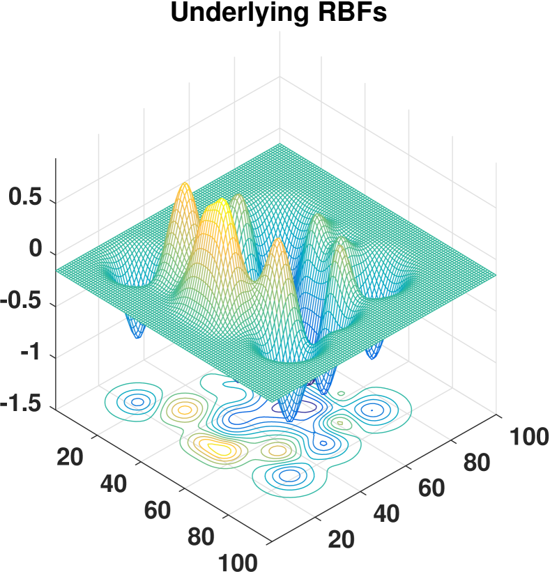
(a)

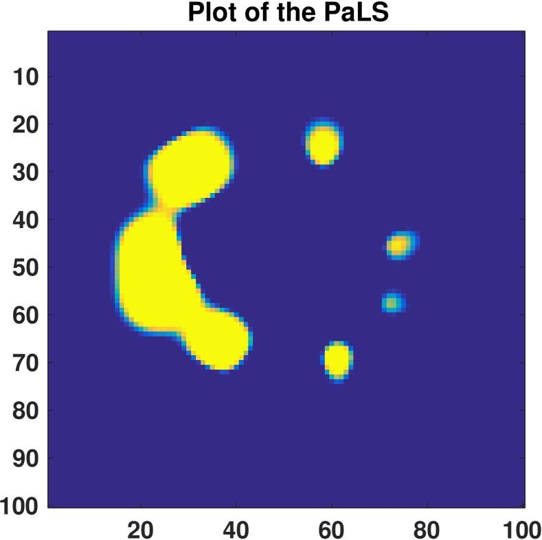
(b)

Figure 1: (a) Surface and contour plot of a test anomaly on $100\times 100$ mesh with 25 basis functions where the cut off is at $c=0.15$. (b) The PaLS function of the test anomaly on the left. If $\phi(\mathbf{x},\mathbf{p})\geq 0.15$, then $\mathbf{x}$ is inside the anomaly (light) and if $\phi(\mathbf{x},\mathbf{p})<0.15$, then $\mathbf{x}$ is outside the anomaly (dark).

Let $n_{d}$, $n_{s}$, and $n_{\omega}$ denote the number of detectors, sources, and frequencies, respectively. The discretization of (2) leads to computed measurements, $\mathbf{m}_{i}(\omega_{j},\mathbf{p})\in\mathbb{C}^{n_{d}}$, for each source term, $\mathbf{b}_{i}$,

(5) $$\mathbf{m}_{i}(\omega_{j},\mathbf{p})=\mathbf{C}^{T}\left(\frac{\imath\omega_{j}}{\nu}\mathbf{E}+\mathbf{A}(\mathbf{p})\right)^{-1}\mathbf{b}_{i},$$

where the rows of $\mathbf{C}^{T}$ correspond to the detectors. $\mathbf{A}(\mathbf{p})$ derives from a finite difference discretization of the diffusion and absorption terms in (2), and $\mathbf{E}$ derives from the frequency term in (2). $\mathbf{E}$ is almost the identity except that it has zero rows for points on the boundary, $x_{3}=0,\>x_{3}=c,$ in (2); so, $\mathbf{E}$ is singular.

For simplicity, we consider the nonlinear residual for a single frequency, $\omega_{j}=0$. In vector form, the residual is defined as follows

(6) $$\mathbf{r}(\mathbf{p})=\begin{bmatrix}\mathbf{r}_{1}(\mathbf{p})\\ \vdots\\ \mathbf{r}_{n_{s}}(\mathbf{p})\\ \end{bmatrix}=\begin{bmatrix}\mathbf{m}_{1}(\mathbf{p})-\mathbf{d}_{1}\\ \vdots\\ \mathbf{m}_{n_{s}}(\mathbf{p})-\mathbf{d}_{n_{s}}\end{bmatrix}=\begin{bmatrix}\mathbf{C}^{T}\mathbf{A}^{-1}(\mathbf{p})\mathbf{b}_{1}-\mathbf{d}_{1}\\ \vdots\\ \mathbf{C}^{T}\mathbf{A}^{-1}(\mathbf{p})\mathbf{b}_{n_{s}}-\mathbf{d}_{n_{s}}\end{bmatrix},$$

where $\mathbf{r}_{i}\in\mathbb{R}^{n_{d}}$, $\mathbf{d}_{i}$ is the data vector with the measurements from the detectors corresponding to source $\mathbf{b}_{i}$, and the nonlinear least squares problem (1) becomes

(7) $$\min_{\mathbf{p}}\frac{1}{2}\|\mathbf{r}(\mathbf{p})\|_{2}^{2}.$$

Let $\mathbf{J}$ be the Jacobian of $\mathbf{r}(\mathbf{p})$,

(8) $$\mathbf{J}=\frac{\partial\mathbf{r}(\mathbf{p})}{\partial\mathbf{p}}=\left[\begin{array}[]{ccc}\displaystyle\frac{\partial\mathbf{r}(\mathbf{p})}{\partial\mathbf{p}_{1}}&\ldots&\displaystyle\frac{\partial\mathbf{r}(\mathbf{p})}{\partial\mathbf{p}_{n_{p}}}\end{array}\right],$$

where the components of $\mathbf{J}$ are given by the small vectors

(9) $$\mathbf{J}_{jk}(\mathbf{p})=\frac{\partial}{\partial\mathbf{p}_{k}}(\mathbf{C}^{T}\mathbf{A}^{-1}(\mathbf{p})\mathbf{b}_{j})=-\mathbf{C}^{T}\mathbf{A}^{-1}(\mathbf{p})\frac{\partial\mathbf{A}(\mathbf{p})}{\partial\mathbf{p}_{k}}\mathbf{A}^{-1}(\mathbf{p})\mathbf{b}_{j}\in\mathbb{R}^{n_{d}}.$$

Evaluating the objective function at $\mathbf{p}$ requires solving $n_{s}\cdot n_{\omega}$ large linear systems. Once $\mathbf{r}(\mathbf{p})$ and $\mathbf{A}^{-1}(\mathbf{p})\mathbf{b}_{j}$ are available, evaluating $\mathbf{J}$ using the co-state approach [29] requires solving an additional $n_{d}\cdot n_{\omega}$ adjoint systems for the detectors. As a result, standard optimization approaches require $O(10^{3}-10^{4})$ large linear system solves at each optimization step. The size of a realistic linear system is at least $O(10^{6})$. This leads to an enormous computational bottleneck, and new computational techniques are needed.

We use TREGS [10] to solve the nonlinear least squares problem (7). The TREGS algorithm combines a trust region method with a regularized minimization of the Gauss-Newton (GN) model [11]. The local (GN) model at the current parameter vector, $\mathbf{p}_{c}$, is given by

(10) $$f(\mathbf{p}_{c}+\boldsymbol{\delta})\approx m_{GN}(\mathbf{p}_{c}+\boldsymbol{\delta})=\frac{1}{2}{\mathbf{r}_{c}}^{T}\mathbf{r}_{c}+\mathbf{r}_{c}^{T}\mathbf{J}_{c}\boldsymbol{\delta}+\frac{1}{2}\boldsymbol{\delta}^{T}{\mathbf{J}_{c}}^{T}\mathbf{J}_{c}\boldsymbol{\delta},$$

and its minimization is equivalent to the least squares problem

(11) $$\min\limits_{\boldsymbol{\delta}}\|\mathbf{J}_{c}\boldsymbol{\delta}+\mathbf{r}(\mathbf{p}_{c})\|_{2}^{2}.$$

The TREGS algorithm favors updates corresponding to (1) the large singular values and (2) the left singular vectors with large components in $\mathbf{r}$ as determined by a generalized cross validation-like (GCV) criterion. Since the Jacobian tends to be ill-conditioned, the emphasis on large singular values leads to relatively small steps that provide relatively large reductions in the GN model (10). We refer the reader to [10] for more details of TREGS.

3 A Randomized Approach

We recast the nonlinear least squares problem as a stochastic optimization problem using randomization to drastically reduce the number of large linear system solves in (6) and (9). The columns of $\mathbf{B}=[\mathbf{b}_{1},\cdots,\mathbf{b}_{n_{s}}]$ are source terms, and we refer to any linear combination of these sources as a simultaneous source. Simultaneous random sources, $\mathbf{B}\mathbf{w}$, with $\mathbf{w}\in\mathbb{R}^{n_{s}}$ a random vector, have been used in several areas [3, 21, 22, 12]. In this section, we introduce the concept of optimized simultaneous sources and detectors to improve the rate of convergence of the optimization and the quality of the inverse solution.

3.1 A Stochastic Optimization Approach

To recast (6)–(7) as a stochastic optimization problem, we first write the residual in matrix form. For a single frequency, we get

(12) $$\mathbf{R}(\mathbf{p})=[\mathbf{r}_{1}(\mathbf{p})\>\>\>\mathbf{r}_{2}(\mathbf{p})\>\>\cdots\>\>\>\mathbf{r}_{n_{s}}(\mathbf{p})]=\mathbf{C}^{T}\mathbf{A}^{-1}(\mathbf{p})\mathbf{B}-\mathbf{D},$$

where the vectors $\mathbf{r}_{i}\in\mathbb{R}^{n_{d}}$ are defined in (6), and consequently $\mathbf{r}(\mathbf{p})=\text{vec}(\mathbf{R}(\mathbf{p}))$. The columns of $\mathbf{D}=[\mathbf{d}_{1},\cdots,\mathbf{d}_{n_{s}}]$ are the measurements corresponding to source $\mathbf{b}_{i}$. We have

(13) $$\min\limits_{\mathbf{p}}\|\mathbf{r}(\mathbf{p})\|_{2}^{2} = \min\limits_{\mathbf{p}}\sum_{j=1}^{n_{s}}\|\mathbf{C}^{T}\mathbf{A}^{-1}(\mathbf{p})\mathbf{b}_{j}-\mathbf{d}_{j}\|_{2}^{2}=\min\limits_{\mathbf{p}}\|\mathbf{C}^{T}\mathbf{A}^{-1}(\mathbf{p})\mathbf{B}-\mathbf{D}\|_{F}^{2}.\mbox{ }$$

Each evaluation of the objective function requires solving $n_{s}\cdot n_{\omega}$ linear systems. Haber et al. [12] reduce this cost using simultaneous random sources combined with (stochastic) trace estimators, following Hutchinson [15].

Let $\mathbf{w}$ be a random vector with mean $\mathbf{0}$ and identity covariance matrix, and let $\mathbb{E}$ denote the expected value with respect to the random vector $\mathbf{w}$. Then

$$\mathbb{E}\left[\mathbf{w}^{T}\mathbf{R}(\mathbf{p})^{T}\mathbf{R}(\mathbf{p})\mathbf{w}\right]=\mathrm{trace}\left(\mathbf{R}(\mathbf{p})^{T}\mathbf{R}(\mathbf{p})\right)=\|\mathbf{R}(\mathbf{p})\|_{F}^{2}.$$

As a particular choice, we choose $\mathbf{w}$ to be a realization from the Rademacher distribution, where each component of $\mathbf{w}$ is independently and identically distributed (i.i.d.) taking values from $\{-1,+1\}$, each with probability $\displaystyle\frac{1}{2}$. Then, as shown in [15], $\mathbf{w}^{T}\mathbf{R}(\mathbf{p})^{T}\mathbf{R}(\mathbf{p})\mathbf{w}$ is a minimum variance and unbiased estimator of the trace of $\mathbf{R}(\mathbf{p})^{T}\mathbf{R}(\mathbf{p})$. Thus, the nonlinear least squares problem can be written as a stochastic minimization problem

(14) $$\min\limits_{\mathbf{p}}\|\mathbf{R}(\mathbf{p})\|_{F}^{2}=\min\limits_{\mathbf{p}}\mathrm{trace}\,\,\mathbf{R}(\mathbf{p})^{T}\mathbf{R}(\mathbf{p})=\min\limits_{\mathbf{p}}\mathbb{E}\left(\mathbf{w}^{T}\mathbf{R}(\mathbf{p})^{T}\mathbf{R}(\mathbf{p})\mathbf{w}\right).$$

For a random vector $\mathbf{w}$ and simultaneous random source $\mathbf{B}\mathbf{w}$, we have

(15) $$\mathbf{R}(\mathbf{p})\mathbf{w}=(\mathbf{C}^{T}\mathbf{A}^{-1}(\mathbf{p})\mathbf{B}-\mathbf{D})\mathbf{w}=\mathbf{C}^{T}\mathbf{A}^{-1}(\mathbf{p})\mathbf{B}\mathbf{w}-\mathbf{D}\mathbf{w}.$$

So, computing $||\mathbf{R}(\mathbf{p})\mathbf{w}||_{2}^{2}\$ requires a single PDE solve rather than $n_{s}$ solves, which drastically reduces the cost of a function evaluation.

In contrast to the approach in [12], we use a Newton-type method, so we also need to reduce the cost of Jacobian evaluations. Therefore, we propose a variation that also drastically reduces the cost of computing $\mathbf{A}^{-T}(\mathbf{p})\mathbf{C}$ for the Jacobian. Let $\mathbf{v}\in\mathbb{R}^{n_{d}}$ and $\mathbf{w}\in\mathbb{R}^{n_{s}}$ with all components i.i.d.  uniformly from $\{-1,+1\}$. Using the well-known cyclic property of the trace [20, p. 110], we get

(16) $$\mathbb{E}\left[\left(\mathbf{v}^{T}\mathbf{R}\mathbf{w}\right)^{2}\right] = \mathbb{E}\left[\left(\mathbf{v}^{T}\mathbf{R}\mathbf{w}\right)\left(\mathbf{w}^{T}\mathbf{R}^{T}\mathbf{v}\right)\right]=\mathbb{E}\left[\mathrm{trace}\left(\mathbf{v}\mathbf{v}^{T}\mathbf{R}\mathbf{w}\mathbf{w}^{T}\mathbf{R}^{T}\right)\right]$$

$$= \mathrm{trace}\left(\mathbb{E}\left(\mathbf{v}\mathbf{v}^{T}\mathbf{R}\mathbf{w}\mathbf{w}^{T}\mathbf{R}^{T}\right)\right)=\mathrm{trace}\left(\mathbf{R}\mathbf{R}^{T}\right)=||\mathbf{R}||_{F}^{2},$$

which requires a single additional adjoint solve rather than an additional $n_{d}$ solves for the Jacobian.

Typically, we need multiple random samples $\mathbf{w}_{j}$ and $\mathbf{v}_{j}$ to make the variance in our stochastic estimates sufficiently small. Hence, we set

(17) $$\mathbf{W}=\frac{1}{\sqrt{\ell_{s}}}(\mathbf{w}_{1}\>\mathbf{w}_{2}\>\cdots\>\mathbf{w}_{\ell_{s}})\;\;\in\mathbb{R}^{n_{s}\times\ell_{s}},$$

where each column vector $\mathbf{w}_{j}$ is i.i.d.  with zero expectation and covariance equal to the identity and $\ell_{s}\ll n_{s}$. Similarly, we set

(18) $$\mathbf{V}=\frac{1}{\sqrt{\ell_{d}}}(\mathbf{v}_{1}\>\mathbf{v}_{2}\>\cdots\>\mathbf{v}_{\ell_{d}})\;\;\in\mathbb{R}^{n_{d}\times\ell_{d}},$$

where each column vector $\mathbf{v}_{j}$ is i.i.d.  with zero expectation and covariance equal to the identity and $\ell_{d}\ll n_{d}$. It is easily verified that these choices give

(19) $$\mathbb{E}[\mathbf{W}\mathbf{W}^{T}]=\mathbf{I}_{n_{s}} \mathbb{E}[\mathbf{V}\mathbf{V}^{T}]=\mathbf{I}_{n_{d}}.$$ and

Next, we replace the sources $\mathbf{B}$ by simultaneous random sources $\mathbf{B}\mathbf{W}$ and the detectors $\mathbf{C}$ by simultaneous random detectors $\mathbf{C}\mathbf{V}$. Assume that $\mathbf{W}$ and $\mathbf{V}$ are independent and we compute unbiased estimates for $\|\mathbf{R}(\mathbf{p})\|^{2}$.

Theorem 3.1.

Let $\mathbf{W}\in\mathbb{R}^{n_{s}\times\ell_{s}}$ and $\mathbf{V}\in\mathbb{R}^{n_{d}\times\ell_{d}}$ be as given above. Let $\mathbf{R}\in\mathbb{R}^{n_{d}\times n_{s}}$. Then

(20) $$\mathbb{E}\left[\|\mathbf{V}^{T}\mathbf{R}\mathbf{W}\|_{F}^{2}\right]=\|\mathbf{R}\|_{F}^{2}.$$

Proof 3.2.

(21) $$\mathbb{E}\left[\|\mathbf{V}^{T}\mathbf{R}\mathbf{W}\|_{F}^{2}\right] = \mathbb{E}\left[\mathrm{trace}\left(\mathbf{W}^{T}\mathbf{R}^{T}\mathbf{V}\mathbf{V}^{T}\mathbf{R}\mathbf{W}\right)\right]=\mathbb{E}\left[\mathrm{trace}\left(\mathbf{W}\mathbf{W}^{T}\mathbf{R}^{T}\mathbf{V}\mathbf{V}^{T}\mathbf{R}\right)\right]$$

$$= \mathrm{trace}\left(\mathbb{E}\left[\mathbf{W}\mathbf{W}^{T}\right]\mathbf{R}^{T}\mathbb{E}\left[\mathbf{V}\mathbf{V}^{T}\right]\mathbf{R}\>\right)=\mathrm{trace}\left(\mathbf{R}^{T}\mathbf{R}\right)=\|\mathbf{R}\|_{F}^{2}.$$

Since TREGS has proven very effective for the nonlinear least squares problem in DOT with PaLS, we continue to use the TREGS algorithm in the stochastic minimization problem

(22) $$\min\limits_{\mathbf{p}}\mathbb{E}\left[||\mathbf{V}^{T}\mathbf{R}(\mathbf{p})\mathbf{W}||^{2}\right]=\min\limits_{\mathbf{p}}||\mathbf{R}(\mathbf{p})||^{2}.$$

We derive the least squares problem used in TREGS to compute a regularized Gauss-Newton update for the stochastic problem as follows. For any $\mathbf{p}$,

(23) $$\mathrm{vec}\left(\mathbf{V}^{T}\mathbf{R}(\mathbf{p})\mathbf{W}\right)=\left(\mathbf{W}^{T}\otimes\mathbf{V}^{T}\right)\mathrm{vec}(\mathbf{R}(\mathbf{p}))=\left(\mathbf{W}^{T}\otimes\mathbf{V}^{T}\right)\mathbf{r}(\mathbf{p});$$

see [14, lemma 4.3.1]. Using a first order approximation to $\mathbf{r}(\mathbf{p}+\boldsymbol{\delta})$ gives

$$\left(\mathbf{W}^{T}\otimes\mathbf{V}^{T}\right)\mathbf{r}(\mathbf{p}+\boldsymbol{\delta})\approx\left(\mathbf{W}^{T}\otimes\mathbf{V}^{T}\right)(\mathbf{r}(\mathbf{p})+\mathbf{J}\boldsymbol{\delta}),$$

which leads to the (sampled) least squares problem

(24) $$\min\limits_{\boldsymbol{\delta}}\|(\mathbf{W}^{T}\otimes\mathbf{V}^{T})\mathbf{J}{\boldsymbol{\delta}}+(\mathbf{W}^{T}\otimes\mathbf{V}^{T})\mathbf{r}(\mathbf{p})\|_{2}^{2},$$

replacing (11). Note that setting up the least squares problem (24) does not require any computations beyond $\mathbf{A}(\mathbf{p})^{-1}(\mathbf{B}\mathbf{W})$ and $\mathbf{A}(\mathbf{p})^{-T}(\mathbf{C}\mathbf{V})$. In addition, (24) has the following desirable properties for the sampled Jacobian and residual, which follow directly from (19) and well-known properties of the Kronecker product.

(25) $$\mathbb{E}\left[\left((\mathbf{W}^{T}\otimes\mathbf{V}^{T})\mathbf{J}\right)^{T}\,(\mathbf{W}^{T}\otimes\mathbf{V}^{T})\mathbf{r}\right] = \mathbf{J}^{T}\mathbb{E}[\mathbf{W}\mathbf{W}^{T}\otimes\mathbf{V}\mathbf{V}^{T}]\mathbf{r}=\mathbf{J}^{T}\mathbf{r},$$

(26) $$\mathbb{E}\left[\left((\mathbf{W}^{T}\otimes\mathbf{V}^{T})\mathbf{J}\right)^{T}\,(\mathbf{W}^{T}\otimes\mathbf{V}^{T})\mathbf{J}\right] = \mathbf{J}^{T}\mathbb{E}\left[\mathbf{W}\mathbf{W}^{T}\otimes\mathbf{V}\mathbf{V}^{T}\right]\mathbf{J}=\mathbf{J}^{T}\mathbf{J}.$$

So, the proposed randomization provides unbiased estimates for the gradient and the Gauss-Newton Hessian.

Two approaches to stochastic optimization are commonly used [26]. One approach, stochastic approximation (SA), uses a new random vector (or small batch of random vectors) in each optimization step. The other approach, sample average approximation (SAA), uses a fixed set of random vectors over multiple (or many) optimization steps. In this paper, we focus on the SAA approach [26] to solve the stochastic problem (22). The SAA approach approximates (22) by the sample average problem. At each iteration, this approach requires solving only $\ell_{s}+\ell_{d}$ linear systems for each frequency to estimate the objective function and the Jacobian rather than $n_{s}+n_{d}$.

We give two representative solutions for our problem using the SAA approach in Figure 2. For DOT, the use of simultaneous random sources and detectors initially leads to good progress. However, later in the iteration the convergence slows down, and in many cases, for our problem, it does not lead to sufficiently accurate solutions. In fact, with the SAA approach, (typically) the residual norm does not reach the noise level, the stopping criterion used (see the discussion of PaLS in Section 2), while the standard optimization using all sources and all detectors does converge to the noise level. We will demonstrate this in Section 4. In the next section, we provide a solution to this problem.

(a)

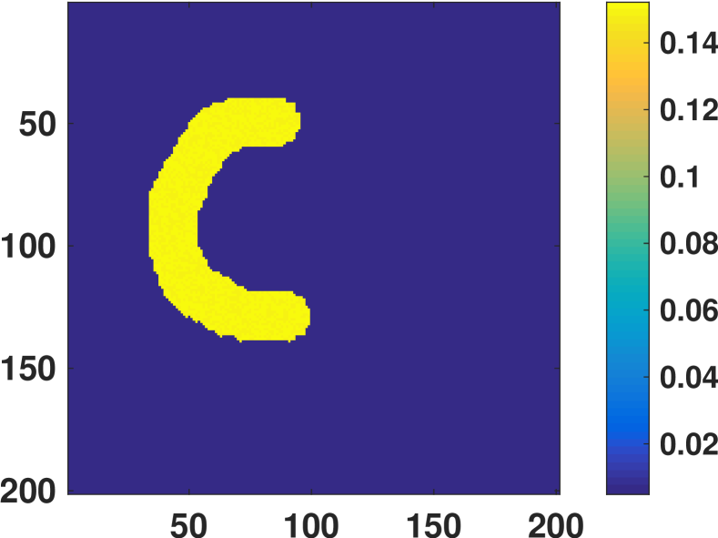
(b)

(c)

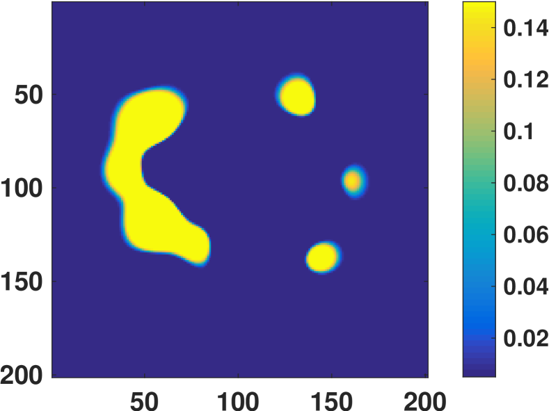
(d)

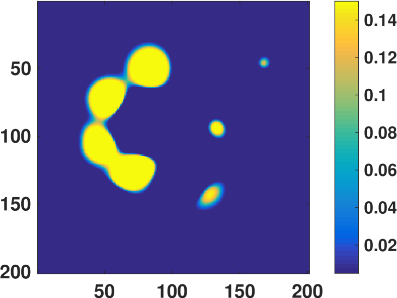
(e)

Figure 2: Reconstruction of a test anomaly on $201\times 201$ mesh with 32 sources, 32 detectors, using only the zero frequency.
(a) Initial configuration with 25 basis functions arranged in a $5\times 5$ grid where 12 basis functions have positive expansion factors (visible as high absorption regions) and 13 basis functions have negative expansion factors (invisible). (b) True shape of the anomaly. (c) Reconstruction using all sources and detectors. (d) & (e) Two reconstruction results using simultaneous random sources and detectors with $\ell_{s}=\ell_{d}=10$.

3.2 Improving the Randomized Approach

In the standard SAA approach, when convergence slows down or a minimum is found for the chosen sample (but not for the true problem), a new sample is chosen to improve the approximate solution. However, for our problem this approach leads to slow convergence and stagnation, unless we obtain more accurate estimates of the dominant singular components of the Jacobian and the corresponding components of the gradient (see also [10]). Hence, after exploiting the relatively fast initial convergence for our problem, we want to avoid stagnation of convergence in the next phase. One approach is to add additional random simultaneous sources and detectors, that is, increase the sample size, as proposed in [25, 6, 5, 23, 24], with good results. However, this requires progressively more, expensive, solves. Therefore, for efficiency, we choose to keep the number of simultaneous sources and detectors fixed. To improve convergence, we exploit the (often fairly good) approximate solution at a chosen modest intermediate tolerance to obtain a small number of simultaneous sources and detectors that are optimized to provide more accurate estimates of the desired derivative information. Since this optimization is local for the current $\mathbf{p}$, we complement these optimized vectors by random simultaneous sources and detectors. We make this precise below.

The nonlinear least squares algorithm TREGS focuses on the dominant singular values of the Jacobian to compute good updates to the parameter vector [10]. The corresponding right singular vectors capture the directions in parameter space of largest sensitivity in the objective function. Hence, we want to update $\mathbf{W}$ and $\mathbf{V}$ so as to best approximate the dominant right singular subspace of $\mathbf{J}$ while respecting the Kronecker product structure in (24). This is important for two reasons. First, for the same (fixed) small number of simultaneous sources and detectors, this gives us locally (at the current $\mathbf{p}$) the best approximation to what TREGS would do using all sources and detectors. Second, the directions corresponding to the dominant right singular vectors are best informed by the data.

So, when a chosen intermediate tolerance is reached, our method computes the full Jacobian $\mathbf{J}$ once, which requires a total of $n_{s}+n_{d}$ solves. Then, we compute a small number, $q_{s}$ respectively $q_{d}$, of orthonormal, optimized simultaneous sources ($\widehat{\mathbf{W}}$) and detectors ($\widehat{\mathbf{V}}$). In practice, small $q_{\mathrm{s}}$ and $q_{\mathrm{d}}$, 2 to 4, seem to be sufficient. We provide some experimental results regarding the number of optimized directions in Section 4. Since $\mathbf{J}$ is typically of rank substantially lower than $n_{\mathrm{p}}$ [1, 10], we expect that computing optimized directions can be done with a cheap approximation to $\mathbf{J}$, for example, computed using the that can be computed at substantially lower cost than solving for all sources and detectors (for each frequency) [13]. However, this is beyond the scope of the current paper.

We would like to maximize

(27) $$\|(\widehat{\mathbf{W}}^{T}\otimes\widehat{\mathbf{V}}^{T})\mathbf{J}\|_{F}^{2}.$$

However, the Kronecker product structure combined with the constraints that $\widehat{\mathbf{W}}$ and $\widehat{\mathbf{V}}$ be isometric matrices leads to a nonlinear constrained optimization problem. For efficiency, we exploit the tensor-structure of this problem, that is, we consider the Jacobian as a third-order array, ${\mathcal{J}}$, with components

(28) $${\mathcal{J}}_{ijk} = \mathbf{c}_{i}^{T}\mathbf{A}^{-1}\frac{\partial\mathbf{A}}{\partial p_{k}}\mathbf{A}^{-1}\mathbf{b}_{j}.$$

This allows us to use an alternating least squares algorithm, a variant of the Higher Order Orthogonal Iteration (HOOI) [8], to find $\widehat{\mathbf{V}}\in\mathbb{R}^{n_{\mathrm{d}}\times q_{\mathrm{d}}}$ and $\widehat{\mathbf{W}}\in\mathbb{R}^{n_{\mathrm{s}}\times q_{\mathrm{s}}}$ that approximately maximize (27); details follow in the next section. The algorithm is only guaranteed to find a local maximum [19, 8]. However, in a number of numerical tests carried out, the tensor algorithm discussed below seems to always converge to the global maximum. A similar observation is reported in [8]. In our experiments, the algorithm also attains the same solutions as MATLAB^®’s fmincon routine, which optimizes for $\widehat{\mathbf{W}}$ and $\widehat{\mathbf{V}}$ simultaneously.

In the remainder of this section, we first discuss computing the optimized simultaneous detectors ($\widehat{\mathbf{V}}$) and sources ($\widehat{\mathbf{W}}$) and then complementing these with random simultaneous sources constrained to $\mathrm{Range}(\widehat{\mathbf{W}})^{\perp}$ and random simultaneous detectors constrained to $\mathrm{Range}(\widehat{\mathbf{V}})^{\perp}$.

3.2.1 Computing Optimized Simultaneous Sources and Detectors

This problem is closely related to the truncated higher-order SVD (HOSVD) [7, 17] or, more precisely, to a truncated Tucker2 decomposition [27, 17], as we do not need truncation in the parameter-derivative direction (the columns of $\mathbf{J}$). As $\widehat{\mathbf{W}}$ and $\widehat{\mathbf{V}}$ are both isometric matrices, so is their Kronecker product, $\mathbf{X}=\widehat{\mathbf{W}}\otimes\widehat{\mathbf{V}}$. Let $[\mathbf{X}\;\mathbf{X}_{c}]$ be a (real) orthogonal matrix, and let $S^{k\times\ell}=\{\mathbf{\Theta}\in\mathbb{R}^{k\times\ell}|\>\mathbf{\Theta}^{T}\mathbf{\Theta}=\mathbf{I}_{\ell}\}$ (the set of all $k\times\ell$ isometric matrices). Then, it follows from standard properties of the Frobenius norm that $\|\mathbf{J}\|_{F}=\|[\mathbf{X}\;\mathbf{X}_{c}]^{T}\mathbf{J}\|_{F}$ and

$$\|\mathbf{J}\|_{F}^{2} = \|\mathbf{X}^{T}\mathbf{J}\|_{F}^{2}+\|\mathbf{X}_{c}^{T}\mathbf{J}\|_{F}^{2}.$$

Since $\|(\mathbf{I}-\mathbf{X}\mathbf{X}^{T})\mathbf{J}\|_{F}=\|\mathbf{X}_{c}^{T}\mathbf{J}\|_{F}$, we have that the maximization problem

(31) $$\arg\max_{\begin{array}[]{c}\widetilde{\mathbf{W}}\in\mathbf{S}^{n_{s}\times\ell_{s}}\\ \widetilde{\mathbf{V}}\in\mathbf{S}^{n_{d}\times\ell_{d}}\end{array}}\|(\widetilde{\mathbf{W}}^{T}\otimes\widetilde{\mathbf{V}}^{T})\mathbf{J}\|_{F}^{2}$$

is equivalent with the minimization problem

$$\arg\min_{\begin{array}[]{c}\widetilde{\mathbf{W}}\in\mathbf{S}^{n_{s}\times\ell_{s}}\\ \widetilde{\mathbf{V}}\in\mathbf{S}^{n_{d}\times\ell_{d}}\end{array}}\|\mathbf{J}-(\widetilde{\mathbf{W}}\otimes\widetilde{\mathbf{V}})(\widetilde{\mathbf{W}}\otimes\widetilde{\mathbf{V}})^{T}\mathbf{J}\|_{F}^{2};$$

see also [8, Theorem 4.1] and [17, p. 477]. We solve the maximization problem by a slight variation of the HOOI algorithm [8] to compute a truncated Tucker2 decomposition [27, 17]. We do not need any compression of the column dimension of $\mathbf{J}$ (the direction corresponding to the parameter derivatives).

We briefly outline the algorithm in tensor form; a MATLAB^® pseudo-code is given in subsection 3.3. Let ${\mathcal{J}}$ be the tensor representation of the Jacobian $\mathbf{J}$, where ${\mathcal{J}}_{ijk}=\mathbf{c}_{i}^{T}\mathbf{A}^{-1}\frac{\partial\mathbf{A}}{\partial p_{k}}\mathbf{A}^{-1}\mathbf{b}_{j}$; the dependence on $\mathbf{p}$ in $\mathbf{A}$, $\mathbf{J}$, and ${\mathcal{J}}$ is suppressed for brevity.

(1) We compute the SVD of the matrix obtained by unfolding the tensor ${\mathcal{J}}$ along its lateral slices ${\mathcal{J}}_{:,j,:}$ and computing the SVD of the resulting matrix $\widetilde{\mathbf{J}}$.

(34) $$\mathbf{U}\mathbf{\Sigma}\mathbf{Y}^{T}=\widetilde{\mathbf{J}} = \left[\begin{array}[]{cccc}{\mathcal{J}}_{:,1,:}&{\mathcal{J}}_{:,2,:}&\cdots&{\mathcal{J}}_{:,n_{s},:}\end{array}\right].$$

Next, we set the initial $\widetilde{\mathbf{V}}=[\mathbf{u}_{1}\;\mathbf{u}_{2}\;\ldots\;\mathbf{u}_{q_{d}}]$ (the leading $q_{d}$ left singular vectors of $\widetilde{\mathbf{J}}$).

Subsequently, we iterate the following two steps until the change in the approximate solution, the tuple $(\widetilde{\mathbf{V}},\widetilde{\mathbf{W}})$, is sufficiently small. (2) Let the tensor ${\mathcal{K}}$ be defined as

$${\mathcal{K}}_{jk\ell}=\sum_{m=1}^{n_{d}}(\widetilde{\mathbf{v}}_{\ell})_{m}{\mathcal{J}}_{m,j,k},\qquad\mbox{for }\ell=1,2,\ldots,q_{d},$$

where the vectors $\widetilde{\mathbf{v}}_{\ell}$ are the columns of $\widetilde{\mathbf{V}}$ ($\ell=1,\ldots,q_{d}$). We compute the SVD of the matrix $\widetilde{\mathbf{K}}$ obtained by unfolding ${\mathcal{K}}$ along its frontal slices ${\mathcal{K}}_{:,:,\ell}$,

(36) $$\mathbf{\Phi}\mathbf{\Omega}\mathbf{\Psi}^{T}=\widetilde{\mathbf{K}} = \left[\begin{array}[]{cccc}{\mathcal{K}}_{:,:,1}&{\mathcal{K}}_{:,:,2}&\cdots&{\mathcal{K}}_{:,:,q_{d}}\end{array}\right],$$

and we set $\widetilde{\mathbf{W}}=[\boldsymbol{\varphi}_{1}\;\boldsymbol{\varphi}_{2}\;\ldots\;\boldsymbol{\varphi}_{q_{s}}]$. (the leading $q_{s}$ left singular vectors of $\widetilde{\mathbf{K}}$)

(3) Define the tensor ${\mathcal{L}}$ by

$${\mathcal{L}}_{ik\ell}=\sum_{m=1}^{n_{s}}(\widetilde{\mathbf{w}}_{\ell})_{m}{\mathcal{J}}_{i,m,k},\qquad\mbox{for }\ell=1,2,\ldots,q_{s},$$

where the vectors $\widetilde{\mathbf{w}}_{\ell}$ are the columns of $\widetilde{\mathbf{W}}$ ($\ell=1,\ldots,q_{s}$). We compute the SVD of the matrix $\widetilde{\mathbf{L}}$ obtained by unfolding ${\mathcal{L}}$ along its frontal slices ${\mathcal{L}}_{:,:,\ell}$,

(38) $$\mathbf{U}\mathbf{\Sigma}\mathbf{Y}^{T}=\widetilde{\mathbf{L}} = \left[\begin{array}[]{cccc}{\mathcal{L}}_{:,:,1}&{\mathcal{L}}_{:,:,2}&\cdots&{\mathcal{L}}_{:,:,q_{s}}\end{array}\right].$$

and we set (the new) $\widetilde{\mathbf{V}}=[\mathbf{u}_{1}\;\mathbf{u}_{2}\;\ldots\;\mathbf{u}_{q_{d}}]$.

Finally, after convergence, we set $\widehat{\mathbf{V}}=\widetilde{\mathbf{V}}$ and $\widehat{\mathbf{W}}=\widetilde{\mathbf{W}}$.

While this procedure gives good approximate solutions, in general only a local maximum of (27) is guaranteed [8]. However, in a number of numerical test carried out, the tensor algorithm seems to always converge to the globally optimal solution. This experience was also reported in [8]. Moreover, we have the following useful result for the case that $\|\mathbf{J}\|_{F}$ can be preserved exactly.

Theorem 3.3.

If isometric matrices $\widetilde{\mathbf{W}}\in\mathbb{R}^{n_{s}\times q_{s}}$ and $\widetilde{\mathbf{V}}\in\mathbb{R}^{n_{d}\times q_{d}}$ exist such that

(39) $$\|(\widetilde{\mathbf{W}}^{T}\otimes\widetilde{\mathbf{V}}^{T})\mathbf{J}\|_{F} = \|\mathbf{J}\|_{F},$$

then, in one iteration, steps (1) – (3) above compute isometric matrices $\widehat{\mathbf{W}}\in\mathbb{R}^{n_{s}\times q_{s}}$ and $\widehat{\mathbf{V}}\in\mathbb{R}^{n_{d}\times q_{d}}$ such that

$$\|(\widehat{\mathbf{W}}^{T}\otimes\widehat{\mathbf{V}}^{T})\mathbf{J}\|_{F} = \|\mathbf{J}\|_{F}.$$

Proof 3.4.

This result follows from the error bound (Property 10) in [7], which in the (matrix) notation of this paper is given by

(40) $$\|\mathbf{J}-(\widetilde{\mathbf{W}}\otimes\widetilde{\mathbf{V}})(\widetilde{\mathbf{W}}\otimes\widetilde{\mathbf{V}})^{T}\mathbf{J}\|_{F}^{2} \leq \sum_{i=q_{d}+1}^{n_{d}}\sigma_{i}^{2}+\sum_{j=q_{s}+1}^{n_{s}}\omega_{j}^{2}.$$

The assumption (39) implies that $\mathrm{Range}(\widetilde{\mathbf{J}})\subseteq\mathrm{Range}(\widetilde{\mathbf{V}})$, which in turn implies that $\mathrm{Rank}(\widetilde{\mathbf{J}})\leq q_{d}$ and hence that $\sigma_{q_{d}+1}=0,\sigma_{q_{d}+2}=0,\ldots,\sigma_{n_{d}}=0$. In a similar fashion, from assumption (39) combined with the choice for $\widetilde{\mathbf{V}}$ from step (1), see (34), it follows that $\mathrm{Range}(\widetilde{\mathbf{K}})\subseteq\mathrm{Range}(\widetilde{\mathbf{W}})$, which implies that $\mathrm{Rank}(\widetilde{\mathbf{K}})\leq q_{s}$ and hence $\omega_{q_{s}+1}=0,\omega_{q_{s}+2}=0,\ldots,\omega_{n_{s}}=0$.
Substitution of $\sigma_{q_{d}+1},\ldots,\sigma_{n_{d}},\omega_{q_{s}+1},\ldots,\omega_{n_{s}}$ into (40) shows that the algorithm will have converged at this point. The algorithm then sets $\widehat{\mathbf{W}}=\widetilde{\mathbf{W}}$ and $\widehat{\mathbf{V}}=\widetilde{\mathbf{V}}$.

Since $\widehat{\mathbf{W}}$ and $\widehat{\mathbf{V}}$ are only optimal at the current $\mathbf{p}$, we complement these optimized simultaneous sources and detectors with a new set of random simultaneous sources and detectors constrained to the orthogonal complement of the span of the optimized directions, keeping the total number of columns in $\mathbf{W}$ and $\mathbf{V}$ the same as before. This procedure can be carried out periodically or for a sequence of prescribed tolerances, but in our experiments it never needs to be done more than once.

3.2.2 Computing Complementary Random Simultaneous Sources and Detectors

We extend the optimized sources and detectors with random simultaneous sources and detectors. Let $\mathbf{W}_{f}=[\widehat{\mathbf{W}}\,\mathbf{W}_{c}]\in\mathbb{R}^{n_{\mathrm{s}}\times n_{\mathrm{s}}}$ and $\mathbf{V}_{f}=[\widehat{\mathbf{V}}\,\mathbf{V}_{c}]\in\mathbb{R}^{n_{\mathrm{d}}\times n_{\mathrm{d}}}$ be orthogonal matrices. We have

(43) $$\|\mathbf{R}(\mathbf{p})\|_{F} = \|\mathbf{V}_{f}^{T}\mathbf{R}(\mathbf{p})\mathbf{W}_{f}\|_{F}$$

$$= \left\|\left[\begin{array}[]{cc}\widehat{\mathbf{V}}^{T}\mathbf{R}(\mathbf{p})\widehat{\mathbf{W}}&\widehat{\mathbf{V}}^{T}\mathbf{R}(\mathbf{p})\mathbf{W}_{c}\\ \mathbf{V}_{c}^{T}\mathbf{R}(\mathbf{p})\widehat{\mathbf{W}}&\mathbf{V}_{c}^{T}\mathbf{R}(\mathbf{p})\mathbf{W}_{c}\end{array}\right]\right\|_{F}$$

The $(1,1)$-block of this matrix can be computed using the known optimized sources and detectors. We estimate the remaining blocks, proceeding more or less as before. We pick random matrices $\mathbf{Y}=(\ell_{s}-q_{s})^{-1/2}[\mathbf{y}_{1}\,\mathbf{y}_{2}\,\ldots\,\mathbf{y}_{\ell_{s}-q_{s}}]$, where each column vector $\mathbf{y}_{j}\in\mathbb{R}^{{\ell_{s}-q_{s}}}$ is i.i.d.  with zero mean and identity covariance and $\mathbf{Z}=(\ell_{d}-q_{d})^{-1/2}[\mathbf{z}_{1}\,\mathbf{z}_{2}\,\ldots\,\mathbf{z}_{\ell_{d}-q_{d}}]$, where each column vector $\mathbf{z}_{j}\in\mathbb{R}^{{n_{d}-q_{d}}}$ is i.i.d.  with zero mean and identity covariance. In our numerical experiments, we again use the Rademacher distribution. Next, we set the new matrices $\mathbf{W}$ and $\mathbf{V}$ to

(44) $$\mathbf{W} = [\widehat{\mathbf{W}}\;(\mathbf{W}_{c}\!\mathbf{Y})],$$

(45) $$\mathbf{V} = [\widehat{\mathbf{V}}\;(\mathbf{V}_{c}\,\mathbf{Z})].$$

We have the following results.

Theorem 3.5.

Let $\mathbf{W}\in\mathbb{R}^{n_{s}\times\ell_{s}}$ and $\mathbf{V}\in\mathbb{R}^{n_{d}\times\ell_{d}}$ be given in (44) and (45), respectively. Let $\mathbf{R}\in\mathbb{R}^{n_{d}\times n_{s}}$. Then,

(46) $$\mathbb{E}[\mathbf{W}\mathbf{W}^{T}] = \mathbf{I}_{n_{s}},$$

(47) $$\mathbb{E}[\mathbf{V}\mathbf{V}^{T}] = \mathbf{I}_{n_{d}},$$

(48) $$\mathbb{E}[\|\mathbf{V}^{T}\mathbf{R}(\mathbf{p})\mathbf{W}\|_{F}^{2}] = \|\mathbf{R}(\mathbf{p})\|_{F}^{2}.$$

Proof 3.6.

For (46), we have

$$\mathbb{E}\left[[\widehat{\mathbf{W}}\;(\mathbf{W}_{c}\!\mathbf{Y})][\widehat{\mathbf{W}}\;(\mathbf{W}_{c}\!\mathbf{Y})]^{T}\right] = \widehat{\mathbf{W}}\widehat{\mathbf{W}}^{T}+\mathbb{E}[\mathbf{W}_{c}\mathbf{Y}\mathbf{Y}^{T}\mathbf{W}_{c}^{T}]$$

$$= \widehat{\mathbf{W}}\widehat{\mathbf{W}}^{T}+\mathbf{W}_{c}\mathbb{E}[\mathbf{Y}\mathbf{Y}^{T}]\mathbf{W}_{c}^{T}=\mathbf{I}_{n_{s}}.$$

An analogous derivation holds for (47). The proof for the last equation follows the proof for Theorem 3.1, using the results above.

As a result of Theorem 3.5, the new $\mathbf{W}$ and $\mathbf{V}$ again give for the expectation of the sampled gradient and the expectation of the sampled Gauss-Newton Hessian the true gradient and Gauss-Newton Hessian,

$$\mathbb{E}[((\mathbf{W}^{T}\otimes\mathbf{V})\mathbf{J})^{T}(\mathbf{W}^{T}\otimes\mathbf{V})\mathbf{r}] = \mathbf{J}^{T}\mathbf{r},$$

$$\mathbb{E}[((\mathbf{W}^{T}\otimes\mathbf{V}^{T})\mathbf{J})^{T}((\mathbf{W}^{T}\otimes\mathbf{V}^{T})\mathbf{J})] = \mathbf{J}^{T}\mathbf{J}.$$

3.3 Implementation

In this section, we first give an algorithm for the computation of optimized simultaneous sources and detectors. Algorithm 3.1 is based on the matrix representation of the Jacobian as defined in (9). Next, we outline the efficient computation of the residual and Jacobian.

Algorithm 3.1 Compute Optimized Sources and Detectors

{ compute $\widetilde{\mathbf{J}}$ and its $q_{d}$ leading left singular vectors }

$\widetilde{\mathbf{J}}$ = [ ]; $\triangleright$ initialize $\widetilde{\mathbf{J}}$ as empty matrix

for  j = 1:$n_{s}$ do

     $\widetilde{\mathbf{J}}=[\widetilde{\mathbf{J}}\;\mathbf{J}_{(j-1)n_{d}+1:jn_{d},1:k}]$ $\triangleright$ add next block from tensor ${\mathcal{J}}$

end for

[$\mathbf{U}$,$\mathbf{\Sigma}$,$\mathbf{Y}$] = SVD($\widetilde{\mathbf{J}}$);  $\widetilde{\mathbf{V}}$ = [$\mathbf{u}_{1}$ $\mathbf{u}_{2}$ … $\mathbf{u}_{q_{d}}$] $\triangleright$ keep $q_{d}$ leading left singular vectors of $\widetilde{\mathbf{J}}$

while not converged do

     { compute $\widetilde{\mathbf{K}}$ and its $q_{s}$ leading left singular vectors }

     $\widetilde{\mathbf{K}}$ = [ ] $\triangleright$ initialize $\widetilde{\mathbf{K}}$ as empty matrix

     for $\ell$ = 1:$q_{d}$ do

         $\widetilde{\mathbf{K}}_{\ell}$ = [ ]

         for j = 1:$n_{s}$ do

              $(\widetilde{\mathbf{K}}_{\ell})_{j,1:k}=\mathbf{v}_{\ell}^{T}\mathbf{J}_{(j-1)n_{d}+1:jn_{d},1:k}$ $\triangleright$ compute row $j$ of $\widetilde{\mathbf{K}}_{\ell}$

         end for

         $\widetilde{\mathbf{K}}=[\widetilde{\mathbf{K}}\;\widetilde{\mathbf{K}}_{\ell}]$ $\triangleright$ add next block of $\widetilde{\mathbf{K}}$

     end for

     [$\mathbf{\Phi}$,$\mathbf{\Omega}$,$\mathbf{\Psi}$] = SVD($\widetilde{\mathbf{K}}$); $\widetilde{\mathbf{W}}=[\boldsymbol{\varphi}_{1}\,\boldsymbol{\varphi}_{2}\,\ldots\,\boldsymbol{\varphi}_{q_{s}}]$ $\triangleright$ keep $q_{s}$ leading left singular vectors of $\widetilde{\mathbf{K}}$

     { compute $\widetilde{\mathbf{L}}$ and its $q_{s}$ leading left singular vectors }

     $\widetilde{\mathbf{L}}$ = [ ]

     for $\ell$ = 1:$q_{s}$ do

         $\widetilde{\mathbf{L}}_{\ell}=\sum_{j=1}^{n_{s}}(\widetilde{\mathbf{w}}_{\ell})_{j}\mathbf{J}_{(j-1)n_{d}+1:jn_{d},1:k}$

         $\widetilde{\mathbf{L}}=[\widetilde{\mathbf{L}}\;\widetilde{\mathbf{L}}_{\ell}]$ $\triangleright$ add next block of $\widetilde{\mathbf{L}}$

     end for

     [$\mathbf{U}$,$\mathbf{\Sigma}$,$\mathbf{Y}$] = SVD($\widetilde{\mathbf{L}}$); $\widetilde{\mathbf{V}}$ = [$\mathbf{u}_{1}$ $\mathbf{u}_{2}$ … $\mathbf{u}_{q_{d}}$] $\triangleright$ keep $q_{d}$ leading left singular vectors of $\widetilde{\mathbf{J}}$

end while

$\widehat{\mathbf{V}}=\widetilde{\mathbf{V}};\;\widehat{\mathbf{W}}=\widetilde{\mathbf{W}}$

We estimate the norm of the residual using

(49) $$(\mathbf{W}^{T}\otimes\mathbf{V}^{T})\mathbf{r}(\mathbf{p})=\begin{bmatrix}\mathbf{V}^{T}\mathbf{C}^{T}\mathbf{A}^{-1}(\mathbf{p})\mathbf{B}\mathbf{w}_{1}-\mathbf{D}\mathbf{w}_{1}\\ \vdots\\ \mathbf{V}^{T}\mathbf{C}^{T}\mathbf{A}^{-1}(\mathbf{p})\mathbf{B}\mathbf{w}_{\ell_{s}}-\mathbf{D}\mathbf{w}_{\ell_{s}}\end{bmatrix}=\begin{bmatrix}\mathbf{V}^{T}\mathbf{C}^{T}\mathbf{z}_{1}-\mathbf{D}\mathbf{w}_{1}\\ \vdots\\ \mathbf{V}^{T}\mathbf{C}^{T}\mathbf{z}_{\ell_{s}}-\mathbf{D}\mathbf{w}_{\ell_{s}}\end{bmatrix},$$

where we solve $\mathbf{A}(\mathbf{p})\mathbf{z}_{i}=\mathbf{B}\mathbf{w}_{i}$ for $\mathbf{z}_{i},\>i=1\cdots\ell_{s}$. This reduces the number of large solves from $n_{s}$ to $\ell_{s}$ per frequency. To compute the Jacobian, we solve the systems, $\mathbf{A}^{T}(\mathbf{p})\mathbf{y}_{j}=\mathbf{C}\mathbf{v}_{j}$ for $\mathbf{y}_{j},\>j=1\cdots\ell_{d}$. This reduces the additional number of large solves from $n_{d}$ to $\ell_{d}$ per frequency. We can use iterative solvers or sparse direct solvers depending on the size of the system [16]. To obtain the $k$-th column of $(\mathbf{W}^{T}\otimes\mathbf{V}^{T})\mathbf{J}$, we compute

(51) $$\left[\begin{array}[]{l}\mathbf{y}_{1}^{T}\frac{\partial\mathbf{A}(\mathbf{p})}{\partial\mathbf{p}_{k}}\mathbf{z}_{1}\cdots\mathbf{y}_{\ell_{d}}^{T}\frac{\partial\mathbf{A}(\mathbf{p})}{\partial\mathbf{p}_{k}}\mathbf{z}_{1}\>\>\mathbf{y}_{1}^{T}\frac{\partial\mathbf{A}(\mathbf{p})}{\partial\mathbf{p}_{k}}\mathbf{z}_{2}\cdots\mathbf{y}_{\ell_{d}}^{T}\frac{\partial\mathbf{A}(\mathbf{p})}{\partial\mathbf{p}_{k}}\mathbf{z}_{\ell_{s}}\\ \end{array}\right]^{T},$$

where $\partial\mathbf{A}(\mathbf{p})/\partial\mathbf{p}_{k}$ is a diagonal matrix if we only invert for absorption. If we also invert for diffusion, this matrix has 5 (in 2D) or 7 (in 3D) diagonals. Moreover, after a few iterations, the changes in $\mathbf{A}(\mathbf{p})$ are highly localized, and $\partial\mathbf{A}(\mathbf{p})/\partial\mathbf{p}_{k}$ contains mostly zero coefficients; see [9]. In that case, we first find the few nonzero components of $\partial\mathbf{A}(\mathbf{p})/\partial\mathbf{p}_{k}$ for each $k$ and the corresponding nonzeros in $\mathbf{z}_{i}$ and $\mathbf{y}_{j}$, and next we efficiently compute $\mathbf{y}_{i}^{T}\frac{\partial\mathbf{A}(\mathbf{p})}{\partial\mathbf{p}_{k}}\mathbf{z}_{j}$ referencing only the few nonzero components in $(\partial\mathbf{A}(\mathbf{p})/\partial\mathbf{p}_{k})\mathbf{z}_{j}$.

4 Numerical Experiments

In this section, we provide two numerical experiments, a 2D and a 3D test case, to demonstrate the effectiveness of combining random simultaneous sources and detectors with optimized simultaneous sources and detectors. The results show that our approach not only produces reconstruction results that are close to those obtained using all sources and all detectors, but it also substantially reduces the computational cost.

Our experimental set up is the same as that in [9], where model reduction was used to reduce the cost of inversion in DOT. The absorption images for the initial sets of parameters for the 2D and 3D experiments are given in Figure 3. For each test case, we construct anomalies in the pixel basis, and we add a small normally distributed random heterogeneity to both the background and the anomaly to make the medium inhomogeneous. We use this pixel-based absorption image to compute the (true) measured data and add $\delta=0.1\%$ white noise to the measured data. This is the same noise level as used in [9]. Then, we reconstruct the absorption images using the PaLS [1] repesentation and TREGS [10] for optimization.

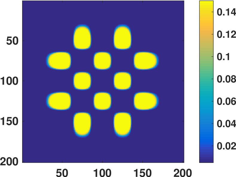
(f)

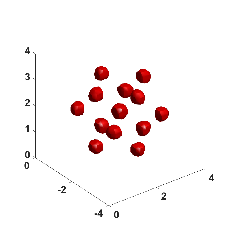
(g)

Figure 3: (a) Initial configuration for the 2D experiment with 25 basis functions arranged in a $5\times 5$ grid, where 12 basis functions have positive expansion factors (visible) and 13 basis functions have negative expansion factors (invisible). (b) Initial configuration for the 3D experiment with 27 basis functions arranged in a $3\times 3\times 3$ grid, where 13 basis functions have positive expansion factors (visible) and 14 basis functions have negative expansion factors (invisible).

2D Experiment. We use a 201$\times$201 grid, which yields $40,401$ unknowns in the discretized PDE (2). The model has 32 sources, 32 detectors, and we use only the zero frequency. Our model has 25 CSRBFs, which leads to 100 parameters (four per 2D basis function) for the nonlinear optimization. We use the same starting guess for each trial (see Figure 3a), with the 25 basis functions arranged in a $5\times 5$ grid, where 12 basis functions have a positive expansion coefficient (visible as high absorption regions) and 13 basis functions have a negative expansion coefficient (invisible).

We use 10 random simultaneous sources and detectors. We update the simultaneous sources and detectors as discussed in Section 3 after a chosen intermediate tolerance has been reached. We find that, in general, the the noise level, $\delta$, is a good choice as the intermediate tolerance: $||\mathbf{r}(\mathbf{p})||_{2}^{2}=\delta$. Since the PaLS representation regularizes the problem, we consider the problem converged when $||\mathbf{r}(\mathbf{p})||_{2}^{2}\leq\delta^{2}$. This is called the discrepancy principle (the factor $\frac{1}{2}$ in (1) is dropped for convenience). We run the 2D experiment for 50 trials. In each trial, the random simultaneous sources and detectors are chosen independently to get representative reconstruction results.

Example 1. The true absorption image for Example 1 is given in Figure 4a. We also include the reconstruction results using all sources and detectors for comparison (see Figure 4b). As can be seen in Figure 4c at the intermediate tolerance, SAA gives a good localization of the anomaly; however, there is little further improvement using SAA (see Figure 2d-e and Figure 5a). Figure 4d-f show that using optimized simultaneous sources and detectors leads to solutions of the same quality as obtained using all sources and detectors. We report the total number of PDE solves required for each approach in Table 1 for a representative result from 50 trials.

While initially the SAA estimate is unbiased, a systematic underestimation of the residual/misfit (bias) [26, Section 5.1.2] arises, since we optimize for a specific small set of random simultaneous sources and detectors. As a result, the algorithm generally stops prematurely. This can make a big difference, since often substantial improvement in the shape of the anomaly occurs towards the end of the optimization. Figure 5 demonstrates how poor the reconstructions using only the SAA approach can be at the convergence tolerance when underestimation of the residual norm is severe. To make a fair comparison in terms of the number of large systems solved, we check the true function evaluation of the SAA approach on the side. Table 2 shows that in terms of the true function evaluation, the SAA approach does not reach the convergence tolerance. Once we use a few optimized sources and detectors, this is no longer an issue (see Table 2).

The main purpose of the SAA approach and our modification is to reduce the large number of discretized PDE solves required for the inversion. In Table 1, we give a comparison of the total number of PDE solves for Example 1. Our approach drastically reduces the number of large-scale linear systems that needs to be solved. Additionally, it substantially improves the reconstruction results of the SAA approach.

(a)

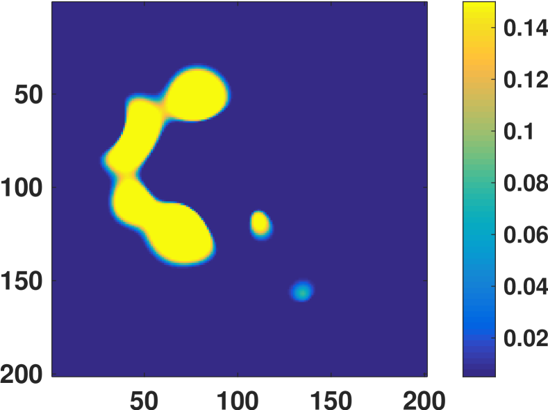
(b)

(c)

(d)

(e)

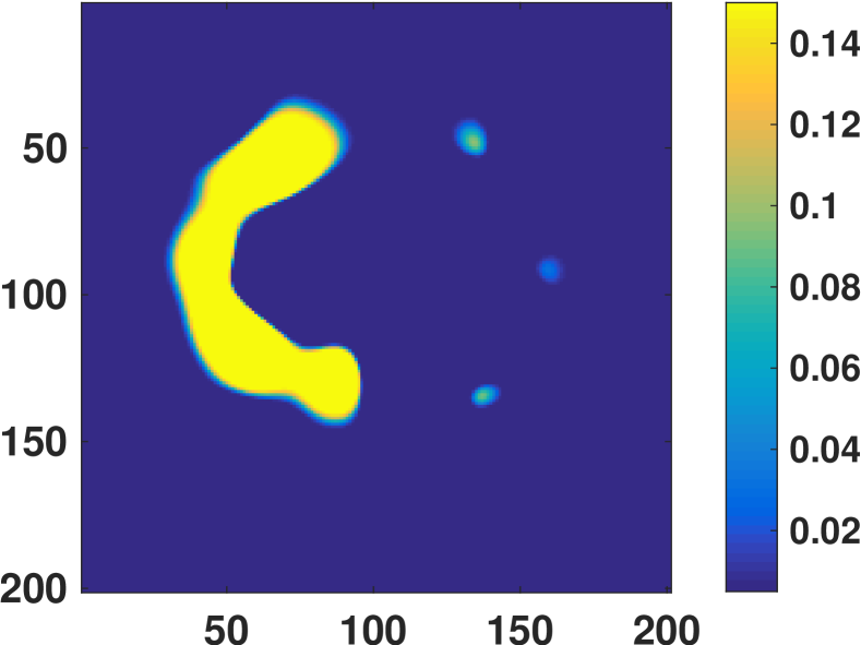
(f)

Figure 4: Results for Example 1. Reconstruction of a test anomaly on $201\times 201$ mesh with 32 sources and detectors, 25 basis functions, and using only the zero frequency. The SAA approach uses 10 random simultaneous sources and detectors.
(a) True shape of the anomaly. (b) Reconstruction using all sources and all detectors. (c) Reconstruction using the SAA approach at a chosen intermediate tolerance. (d) Reconstruction with SAA and 1 optimized simultaneous source and detector. (e) Reconstruction with SAA and 2 optimized simultaneous sources and detectors. (f) Reconstruction with SAA and 3 optimized simultaneous sources and detectors.

	Iteration Number	Function Evaluations	Jacobian Evaluations	Total PDE Solves	Tol
SAA⋆ (intermediate tol)	10	11	6	170	$\delta$
1 Opt simult src/det	18	19	10	524	$\delta^{2}$
2 Opt simult srcs/dets	18	19	10	524	$\delta^{2}$
3 Opt simult srcs/dets	16	17	8	484	$\delta^{2}$
All srcs/All dets	71	72	47	3808	$\delta^{2}$
SAA⋆⋆	(32)	(33)	(19)	(520)	$\delta^{2}$
SAA ⋆⋆⋆	(92)	(93)	(67)	(1700)	$\delta^{2}$

Table 1: Example 1 Results. The total number of iterations, function evaluations, Jacobian evaluations and PDE solves required on average for 50 trials to reach the stopping criterion, $\|\mathbf{r}(\mathbf{p})\|_{2}^{2}=\delta^{2}$.
^⋆The first row gives the cost to reach the intermediate tolerance for the SAA approach, $\|\mathbf{r}(\mathbf{p})\|_{2}^{2}=\delta$. ^⋆⋆ Since the SAA estimate becomes biased and underestimates the objective function, the algorithm stops prematurely. ^⋆⋆⋆The SAA approach measuring the convergence with the true objective function. Parentheses indicate that the SAA approach does not reach the tolerance.

SAA Approach			Rand $\&$ Optimized Simult Src/Det
Iter	True $\|\mathbf{r}\|_{2}^{2}$ ($\delta^{2}$)	Estimated $\|\mathbf{r}\|_{2}^{2}$ ($\delta^{2}$)	Iter	True $\|\mathbf{r}\|_{2}^{2}$ ($\delta^{2}$)	Estimated $\|\mathbf{r}\|_{2}^{2}$ ($\delta^{2}$)
1	118940	38820	1-5	(SAA)⋆	(SAA)⋆
6	1192.5	391.15	6	1194.9	1197.3
11	56.550	22.575	13	118.73	118.56
15	3.748	0.8650	16	19.894	19.929
(99)	$-$	$-$	22	0.8403	0.8389

Table 2: Subset of results for Example 1. The comparison of the true objective function $\|\mathbf{r}\|_{2}^{2}$ and its SAA estimate relative to the stopping criterion ($\delta^{2}$) for selected iterations. For the SAA approach, the estimated residual is obtained with 10 random simultaneous sources and detectors. Parentheses indicate that the SAA approach does not reach the tolerance. The estimated residual norms using random and optimized simultaneous sources and detectors are obtained using 3 optimized simultaneous sources and detectors. (SAA)^⋆ indicates that we initially use the SAA approach up to the intermediate tolerance.

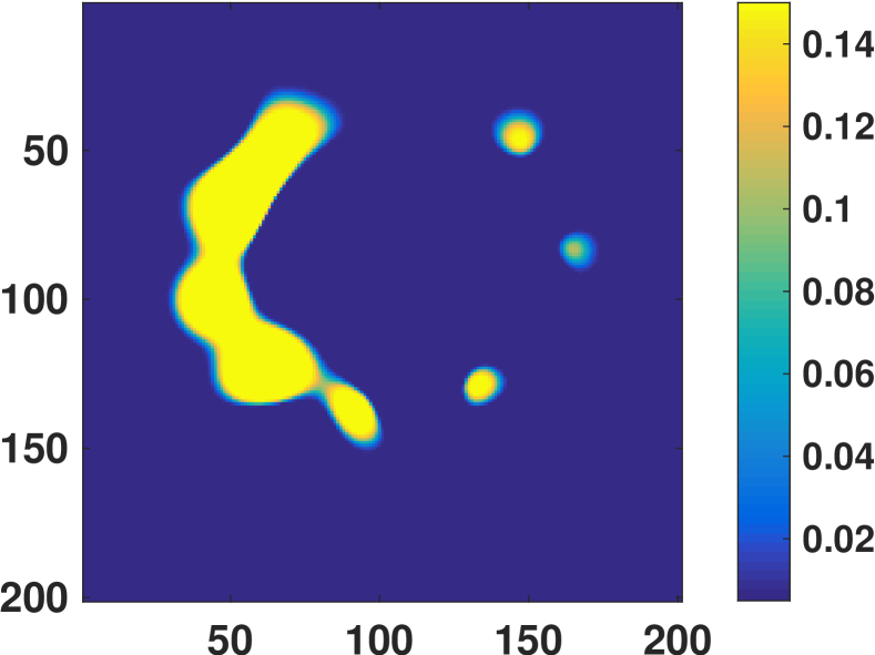
(g)

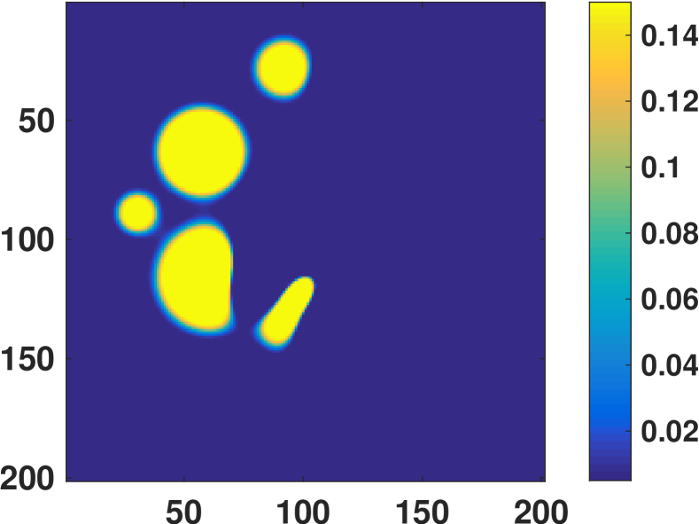
(h)

Figure 5: Two examples of poor SAA reconstructions for the 2D problem after the maximum number of iterations. Reconstruction of a test anomaly on $201\times 201$ mesh with 32 sources and detectors, 25 basis functions, and using only the zero frequency.

3D Experiment. We use a $32\times 32\times 32$ grid, which gives $32,768$ unknowns in the discretized PDE (2). The model has 225 sources at the top and 225 detectors on the bottom, and we use only the zero frequency. In the PaLS approach, we use 27 CSRBFs, which leads to 135 parameters (five per 3D basis function) for the nonlinear optimization. The absorption image using the initial set of parameters is given in Figure 3b where 13 basis functions have a positive expansion coefficient (visible as high absorption regions) and 14 basis functions have a negative expansion coefficient (invisible). In our approach, we use only 12 random simultaneous sources and detectors.

Example 2. The true absorption image for Example 2 is given in Figure 6a. The reconstruction using all sources and detectors is given in Figure 6b. Figure 6c shows that SAA approach gives a good localization of the anomaly at the intermediate tolerance. However, little further improvement appears using the SAA approach, even after the maximum iterations; see Figure 6d. In Figure 6e-g, we show the reconstruction results when combining random and optimized simultaneous sources and detectors.

The straightforward inversion using all sources and detectors requires $9,225$ large linear solves. Table 3 shows that our approach reduces the number of large linear solves by about a factor 12 compared with using all sources and detectors, while approximating the original shape well. Clearly, there is a large improvement to be gained by using a small number of optimized simultaneous sources and detectors. For larger problems with many sources and detectors and using multiple frequencies, we expect much larger gains.

Overall, our approach improves the rate of convergence of the optimization and reduces the number of large-scale linear systems solves. Moreover, combining random and optimized simultaneous sources and detectors improves the quality of the inverse solution.

(a)

(b)

(c)

(d)

(e)

(f)

Figure 6: Results for Example 2. Reconstruction of a test anomaly on a $32\times 32\times 32$ mesh with 225 sources and detectors, 27 basis functions, and using only the zero frequency. The SAA approach uses 15 random simultaneous sources and detectors.
(a) True shape of the anomaly. (b) Reconstruction using all sources and all detectors. (c) Reconstruction using the SAA approach at the intermediate tolerance. (d) Reconstruction using the SAA approach after the maximum iterations. (e) Reconstruction with SAA and 2 optimized simultaneous sources and detectors. (f) Reconstruction with SAA and 4 optimized simultaneous sources and detectors.

	Iteration Number	Function Evaluations	Jacobian Evaluations	Total PDE Solves	Tol
SAA⋆ (intermediate tol)	4	5	6	132	$\delta$
2 Opt simult srcs/dets	12	13	6	726	$\delta^{2}$
4 Opt simult srcs/dets	9	10	3	762	$\delta^{2}$
All srcs/All dets	25	26	15	9225	$\delta^{2}$
SAA ⋆⋆	(99)	(100)	(67)	(2505)	$\delta^{2}$

Table 3: Example 2 Results. The total number of iterations, function evaluations, Jacobian evaluations and PDE solves required to reach the stopping criterion, $\|\mathbf{r}(\mathbf{p})\|^{2}_{2}=\delta^{2}$.
^⋆The first row gives the costs to reach the intermediate tolerance for the SAA approach, $\|\mathbf{r}(\mathbf{p})\|_{2}^{2}=\delta$. ^⋆⋆The SAA approach measuring the convergence with the true objective function. Parentheses indicate that the SAA approach does not reach the tolerance.

5 Conclusions and Future Work

We use the SAA approach to estimate the objective function, the Jacobian, and the gradient using only a few simultaneous random sources and detectors in DOT problems. While this approach is reasonably effective for the application in [12], it does not work quite that well for DOT. Since convergence slows down in later iterations before the noise level is reached, and the standard SAA approach regularly does not converge to the noise level, we propose using optimized simultaneous sources and detectors. With the addition of optimized directions, we observe faster convergence, good quality reconstructions, and robustness. This technique could be quite useful in other applications as well.

Several further improvements should be considered in the future. In particular, approximating the, typically low rank, Jacobian at low cost but sufficiently accurately to compute effective optimized simultaneous sources and detectors would lead to a further substantial reduction in the number of large linear solves. Potentially, computing such a low rank approximation can be combined more efficiently with the tensor form of the Jacobian.

Although our approach has proved successful experimentally, we aim to understand the underlying theory better. In the future, we plan to analyze, more fundamentally, what are the most effective simultaneous sources and detectors for fast convergence of the inverse problem: randomized, optimized (and in what sense), and their combination. An alternative approach to improve convergence, studied in multiple papers [25, 6, 5, 23, 24], is to slowly increase the sample size as the optimization progresses or dynamically choose the sample size. In future work, we plan to compare these approaches with the approach proposed in this paper. We also plan to test and evaluate SA approaches for inversion in DOT.

We intend to update the TREGS algorithm and study how small we can make the number of simultaneous sources and detectors (random and optimized) and still obtain good solutions and fast convergence. Moreover, finding more appropriate stopping criteria for the randomized approach may also improve our results.

As shown in [9], using parametrized interpolatory model reduction can also reduce the cost of inversion for DOT. We plan to combine model reduction with the randomized approach.

6 Acknowledgements

We sincerely thank the reviewers for many helpful suggestions that substantially improved this paper.

References

- [1] A. Aghasi, E. Miller, and M. E. Kilmer. Parametric level set methods for inverse problems. SIAM Journal on Imaging Science, 4(2):618–650, 2011.
- [2] S. R. Arridge. Optical tomography in medical imaging. Inverse Problems, Vol. 16:R41–R93, 1999.
- [3] C. J. Beasley. A new look at marine simultaneous sources. Leading Edge, 27:914–917, 2008.
- [4] D. Boas, D. Brooks, E. Miller, C. DiMarzio, M. Kilmer, R. Gaudette, and Q. Zhang. Imaging the body with diffuse optical tomography. IEEE Signal Processing Magazine, 18(6):57–75, 2001.
- [5] R. Bollapragada, R. Byrd, and J. Nocedal. Exact and inexact subsampled Newton methods for optimization. arXiv preprint arXiv:1609.08502, 2016.
- [6] R. H. Byrd, G. M. Chin, J. Nocedal, and Y. Wu. Sample size selection in optimization methods for machine learning. Mathematical programming, 134(1):127–155, 2012.
- [7] L. de Lathauwer, B. de Moor, and J. Vandewalle. A multilinear singular value decomposition. SIAM Journal on Matrix Analysis and Applications, 21(4):1253 – 1278, 2000.
- [8] L. de Lathauwer, B. de Moor, and J. Vandewalle. On the best rank-1 and rank- approximation of higher-order tensors. SIAM Journal on Matrix Analysis and Applications, 21(4):1324–1342, 2000.
- [9] E. de Sturler, S. Gugercin, M. E. Kilmer, S. Chaturantabut, C. Beattie, and M. O’Connell. Nonlinear parametric inversion using interpolatory model reduction. SIAM J. Sci. Comput, 37(3):B495–B517, 2015.
- [10] E. de Sturler and M. E. Kilmer. A regularized Gauss-Newton trust region approach to imaging in diffuse optical tomography. SIAM J. Sci. Comput., 33:3057 – 3086, 2011.
- [11] J. Dennis and R. Schnabel. Numerical methods for unconstrained optimization and nonlinear equations. SIAM, 1996.
- [12] E. Haber, M. Chung, and F. Herrmann. An effective method for parameter estimation with PDE constraints with multiple right-hand sides. SIAM J. Optim., 22(3):739–757, 2012.
- [13] N. Halko, P. G. Martinsson, and J. A. Tropp. Finding structure with randomness: Probabilistic algorithms for constructing approximate matrix decompositions. SIAM Review, 53(2):217–288, 2011.
- [14] R. A. Horn and C. R. Johnson. Topics in Matrix Analysis. Cambridge University Press, 1991.
- [15] M. F. Hutchinson. A stochastic estimator of the trace of the influence matrix for Laplacian smoothing splines. Commun. Statist. Simulation Comput., 18(3):1059–1076, 1990.
- [16] M. E. Kilmer and E. de Sturler. Recycling subspace information for diffuse optical tomography. SIAM J. Sci. Comput., 27(6):2140–2166, 2006.
- [17] T. G. Kolda and B. W. Bader. Tensor decompositions and applications. SIAM Review, 51(3):455–500, 2009.
- [18] J. R. Krebs, J. E. Anderson, D. Hinkley, R. Neelamani, S. Lee, A. Baumstein, and M.-D. Lacasse. Fast full-wavefield seismic inversion using encoded sources. Geophysics, 74(6):WCC177–WCC188, 2009.
- [19] P. M. Kroonenberg and J. de Leeuw. Principal component analysis of three-mode data by means of alternating least squares algorithms. Psychometrika, 1:69–97, Mar. 1980.
- [20] C. D. Meyer. Matrix Analysis and Applied Linear Algebra. SIAM, 2000.
- [21] S. A. Morton and C. C. Ober. Faster shot-record depth migrations using phase encoding. 68th Annual International Meeting, Society of Exploration Geophysicists, Expanded Abstracts, 37:1131–1134, 1998.
- [22] R. Neelamani, C. E. Krohn, J. R. Krebs, J. K. Romberg, M. Deffenbaugh, and J. E. Anderson. Efficient seismic forward modeling using simultaneous random sources and sparsity. Geophysics, 75(6):WB15–WB27, 2010.
- [23] F. Roosta-Khorasani and M. W. Mahoney. Sub-sampled Newton methods I: Globally convergent algorithms. arXiv preprint arXiv:1601.04737, 2016.
- [24] F. Roosta-Khorasani and M. W. Mahoney. Sub-sampled Newton methods II: Local convergence rates. arXiv preprint arXiv:1601.04738, 2016.
- [25] F. Roosta-Khorasani, K. van den Doel, and U. Ascher. Stochastic algorithms for inverse problems involving PDEs and many measurements. SIAM J. Sci. Comput., 36(5):S3–S22, 2014.
- [26] A. Shapiro, D. Dentcheva, and A. Ruszczyński. Lectures on Stochastic Programming: Modeling and Theory. SIAM, 2009.
- [27] L. R. Tucker. Some mathematical notes on three-mode factor analysis. Psychometrika, 31:279–311, 1966.
- [28] T. van Leeuwen, A. Y. Aravkin, and F. J. Herrmann. Seismic waveform inversion by stochastic optimization. International Journal of Geophysics, 2011.
- [29] C. R. Vogel. Computational Methods for Inverse Problems. SIAM, Philadelphia, 2002.