Centralized Multi-Node Repair Regenerating Codes

Abstract

In a distributed storage system, recovering from multiple failures is a critical and frequent task that is crucial for maintaining the system’s reliability and fault-tolerance. In this work, we focus on the problem of repairing multiple failures in a centralized way, which can be desirable in many data storage configurations, and we show that a significant repair traffic reduction is possible. First, the fundamental tradeoff between the repair bandwidth and the storage size for functional repair is established. Using a graph-theoretic formulation, the optimal tradeoff is identified as the solution to an integer optimization problem, for which a closed-form expression is derived. Expressions of the extreme points, namely the minimum storage multi-node repair (MSMR) and minimum bandwidth multi-node repair (MBMR) points, are obtained. Second, we describe a general framework for converting single erasure minimum storage regenerating codes to MSMR codes. The repair strategy for $e$ failures is similar to that for single failure, however certain extra requirements need to be satisfied by the repairing functions for single failure. For illustration, the framework is applied to product-matrix codes and interference alignment codes. Furthermore, we prove that the functional MBMR point is not achievable for linear exact repair codes. We also show that exact-repair minimum bandwidth cooperative repair (MBCR) codes achieve an interior point, that lies near the MBMR point, when $k\equiv 1\mod e$, $k$ being the minimum number of nodes needed to reconstruct the entire data. Finally, for $k>2e,e\mid k$ and $e\mid d$, where $d$ is the number of helper nodes during repair, we show that the functional repair tradeoff is not achievable under exact repair, except for maybe a small portion near the MSMR point, which parallels the results for single erasure repair by Shah et al.

I Introduction

Ensuring data reliability is of paramount importance in modern storage systems. Reliability is typically achieved through the introduction of redundancy. Traditionally, simple replication of data has been adopted in many systems. For instance, Google file systems opted for a triple replication policy [3]. However, for the same redundancy factor, replication systems fall short on providing the highest level of reliability. On the other hand, erasure codes can be optimal in terms of the redundancy-reliability tradeoff. In erasure codes, a file of size $\mathcal{M}$ is divided into $k$ fragments, each of size $\frac{\mathcal{M}}{k}$. The $k$ fragments are then encoded into $n$ fragments using an $(n,k)$ maximum distance separable (MDS) code and then stored at $n$ different nodes. Using such a scheme, the data is guaranteed to be recovered from any $n-k$ node erasures, providing the highest level of worst-case data reliability for the given redundancy. However, traditional erasure codes suffer from high repair bandwidth. In the case of a single node erasure, they require downloading the entire data of size $\mathcal{M}$ to repair a single node storing a fragment of size $\frac{\mathcal{M}}{k}$. This expansion factor made erasure codes impractical in some applications using distributed storage systems. In the last decade, the repair problem has gained increasing interest and motivated the research for a new class of erasure codes with better repair capabilities. The seminal work in [4] proposed regenerating codes that optimally solve the repair bandwidth problem. Interestingly, the authors in [4] proved that one can significantly reduce the amount of bandwidth required for repair and the bandwidth decreases as each node stores more information. Formally, suppose any $k$ out of $n$ nodes are sufficient to recover the entire file of size $\mathcal{M}$. Assuming that $d$ nodes, termed helpers, participate in the repair process, denoting the storage capacity of each node by $\alpha$ and the amount of information downloaded from each helper by $\beta$, then, an optimal $(\mathcal{M},n,k,d,\alpha,\beta)$ regenerating code satisfies

$$\mathcal{M}=\sum_{i=0}^{k-1}\min\{\alpha,(d-i)\beta\}.$$ (1)

Equation (1) describes the fundamental tradeoff between the storage capacity $\alpha$ and the bandwidth $\beta$. Two extreme points can be obtained from the tradeoff. Minimum storage regenerating (MSR) codes correspond to the best storage efficiency with $\alpha=\frac{\mathcal{M}}{k}$, while minimum bandwidth regenerating (MBR) codes achieve the lowest possible bandwidth at the expense of extra storage per node.

If we recover the exact same information as the failed node, we call it exact repair, otherwise we call it functional repair. Using network coding [5, 6], it is possible to construct functional regenerating codes satisfying (1) [4]. Following the seminal work in [4], there has been a flurry of interest in designing exact-repair regenerating codes that achieve the optimal tradeoff, focusing mainly on the extreme MSR and MBR points, e.g., [7, 8, 9, 10, 11, 12, 13, 14, 15, 16]. For interior points that are between the MBR and MSR points in the tradeoff of (1), [17] showed that most points are not achievable for exact repair. Moreover, there has been a growing literature focused on understanding the fundamental limits of exact-repair regenerating codes. Other outer bounds for exact repair include [18, 19, 20] for general parameters, and [21] for linear codes. The aforementioned references, as most of the studies on regenerating codes in the literature, focus on the single erasure repair problem. However, in many practical scenarios, such as in large scale storage systems, multiple failures are more frequent than a single failure. Moreover, many systems (e.g., [22]) apply a lazy repair strategy, which seeks to limit the repair cost of erasure codes. Instead of immediately repairing every single failure, a a lazy repair strategy waits until $e$ erasures occur, $e\leq n-k$, then, the repair is done by downloading the equivalent of the total information in the system to regenerate the erased nodes. However, a natural question of interest is, whether one can reduce the amount of download in such scenarios.

In this work, we consider centralized repair. Indeed, there are situations in which, due to architectural constraints, it is more desirable to regenerate the lost nodes at a central server before dispatching the regenerated content to the replacement nodes [22]. For instance, one can think of a rack-based node placement architecture [23] in which failures frequently occur to nodes corresponding to a particular rack. In this scenario, a centralized repair of the entire rack is favorable as opposed to repairing the rack on a per-node basis. Furthermore, [23] showed that a centralized repair framework can have interesting applications in communication-efficient secret sharing. Finally, centralized repair can be used in a broadcast network, where the repair information is transmitted to all replacement nodes (e.g. [24]).

Our centralized repair framework requires the content of any $k$ out of $n$ nodes in the system to be sufficient to reconstruct the entire data. Upon the failure of $e$ nodes in the system, the repair is carried out by contacting any $d$ helpers out of the $n-e$ available nodes, $d\leq n-e$, and downloading $\beta$ amount of information from each of the $d$ helpers. Our objective is to characterize the functional repair tradeoff between the storage per node $\alpha$ and the repair bandwidth $\beta$ under the centralized multiple failure repair framework. We also seek to investigate the achievability of the functional tradeoff under exact repair.

I-A Related work

Cooperative regenerating codes (also known as coordinated regenerating codes) have been studied to address the repair of multiple erasures [25, 26] in a distributed manner. In this framework, each replacement node downloads information from $d$ helpers in the first stage. Then, the replacement nodes exchange information between themselves before regenerating the lost nodes. Cooperative regenerating codes that achieve the extreme points on the cooperative tradeoff have been developed; namely, minimum storage cooperative regenerating (MSCR) codes [27, 26, 28] and minimum bandwidth cooperative regeneration (MBCR) codes[29].

The number of nodes involved in the repair of a single node, known as locality, is another important measure of node repair efficiency [30]. Various bounds and code constructions have been proposed in the literature [30, 31]. Recent works have investigated the problem of multiple node repair under locality constraints [32, 33].

The problem of centralized repair has been considered in [14], in which the authors restricted themselves to MDS codes, corresponding to the point of minimum storage per node. [14] showed the existence of MDS codes with optimal repair bandwidth in the asymptotic regime where the storage per node (as well as the entire information) tends to infinity. In [34], the authors proved that Zigzag codes, which are MDS codes designed initially for repairing optimally single erasures [15], can also be used to optimally repair multiple erasures in a centralized manner. In [23], the authors independently proved that multiple failures can be repaired in Zigzag codes with optimal bandwidth. Moreover, [23] defines the minimum bandwidth multi-node repair codes as codes satisfying the property of having the downloaded information $d\beta$ matching the entropy of $e$ nodes. Based on that, the authors derived a lower bound on $\beta$ for systems having a certain entropy accumulation property and then showed achievability of the minimum bandwidth codes using MBCR codes. However, the optimal storage size per node $\alpha$ is not known under these conditions. In [35], the authors presented an explicit MDS code construction that provides optimal repair for all $e\leq n-k$ and $k\leq d\leq n-e$ simultaneously. The authors in [24] studied the problem of broadcast repair for wireless distributed storage which is equivalent to the model we study in this paper. It is worth pointing out that the previous constructions are for high-rate codes, with large subpacketization $\alpha$. In [36], the authors presented an approach that enables single erasure MSR codes to recover from multiple failures simultaneously with near-optimal bandwidth. Based on simulations, [36] showed that their approach can provide efficient recovery of most of the failure patterns, but not all of them. The repair problem of Reed Solomon codes has been recently investigated in [37] for single erasure and in [38, 39, 40, 41] for multiple erasures. In [42], the authors proved that the interference alignment MSR construction of [8], originally designed for repairing any single node failure, can recover from multiple failures in a cooperative way. Specifically, it is shown that any set of systematic nodes, set of parity-check nodes, or pair of nodes can be repaired cooperatively with optimal bandwidth.

I-B Contributions of the paper

The main contributions of this paper are the characterization of functional tradeoff, and the examination of its achievability under exact repair for the extreme points and the interior points. They are summarized as follows.

• We first establish the explicit functional tradeoff between the repair bandwidth and the storage size for functional repair (Theorems 1, 2, 3). We obtain the tradeoff using information flow graphs. From the functional tradeoff, we characterize the minimum storage multi-node repair (MSMR) point, and the minimum bandwidth multi-node repair (MBMR) point.

• When the number of erasures $e$ satisfies $e\geq k$, $k$ being the minimum number of nodes needed to reconstruct the entire data, the tradeoff reduces to a single point, for which we provide an explicit code construction.

• We formalize a construction for exact-repair MSMR codes. Given an instance of an exact linear MSR code, we present a framework to construct an instance of an exact linear MSMR regenerating code. We note here that [27] and [36] used a similar approach for MSCR codes and their numerical results, respectively. Based on this framework, we study the product-matrix (PM) MSR codes [43] and the interference alignment (IA) construction in [8]. We prove the existence of PM and IA MSMR codes for any number of failures $e$, $e\leq n-k$ (Theorems 4, 5, 9). Moreover, for the IA code, we prove that the code can always efficiently recover from any set of $e\leq n-k$ node failures as long as the failed nodes are either all systematic nodes or all parity nodes (Theorem 6); for failures including both systematic and parity nodes, we derive explicit design conditions under which exact recovery is ensured, for some particular system parameters (Theorems 7, 8). We note here that unlike previous constructions, our codes are applicable when the code rate is low and they use a small subpacketization size of $\alpha=k-1$ or $k$.

• We prove that, to our surprise, functional MBMR point is not achievable for linear exact repair codes for $1<e<k$ (Theorems 10, 11), while linear codes achieve such point for single erasure [43].

• We show that exact-repair MBCR codes achieve an interior point, that lies near the MBMR point, when $k\equiv 1\mod e$ (Theorem 12).

• We show that the functional repair tradeoff is not achievable under exact repair for interior points between MBMR and MSMR points, except for maybe a small portion near the MSMR point, for $k,d$ being multiples of $e$ and $k>2e$ (Theorems 13, 14), which parallels the results for single erasure repair [17]. The achievability of the functional tradeoff under exact repair is summarized in Table I.

• Finally, we study the adaptive repair problem of multiple erasures in MBR codes and present an MBR construction with optimal repair, simultaneously for varying numbers of helpers and varying numbers of erasures (Theorem 15).

	MSMR point	MBMR point	Interior points
$e=1$	$\checkmark$ [15, 8, 43]	$\checkmark$ [43]	✗, except maybe for a small portion near the MSMR point [17].
$1<e<k$	$\checkmark$ [35, 14], [Sections III-B, III-C, III-D]	✗ (for linear codes) [Section IV]	$\bullet$ if $k\equiv 1\mod e$: an interior point near the MBMR point is achievable [Section IV-D]. $\bullet$ if $e\mid k,e\mid d,k>2e:$ ✗, except maybe for a small portion near the MSMR point [Section V].
$e\geq k$	$\checkmark$ Section III-A	$\checkmark$Section III-A	$\checkmark$ Section III-A

TABLE I: Summary of achievability results of functional repair tradeoff under exact repair for an $(n,k,d,e,\alpha,\beta)$ distributed storage system. MSMR and MBMR points are defined to be the minimum storage point and the minimum bandwidth point on the functional tradeoff, respectively. Here $e\mid k,e\mid d$ means that $k,d$ are multiples of $e$. The symbol $\checkmark$ denotes achievability while ✗ denotes non-achievability, both of which are under exact repair.

I-C Organization of the paper

The remainder of the paper is organized as follows. In Section II, we first describe the system model before analyzing the fundamental functional repair tradeoff between the storage size and the repair bandwidth. Section III describes our code construction for the case $e\geq k$, as well as the MSMR codes framework and its application to the product-matrix and the interference alignment codes. We prove the non-achievability of MBMR point under linear exact repair in Section IV. The non-achievability of the interior points under exact repair is investigated in Section V. The adaptive repair of multiple erasures for an MBR code is presented in Section VI and Section VII draws conclusions.

Notation. $[n]$ denotes the set of elements $\{1,\ldots,n\}$. $\lceil\cdot\rceil$ and $\lfloor\cdot\rfloor$ represent the ceiling and the floor functions. For a set $\mathcal{A}$, $\mathcal{A}\backslash\{i\}$ denotes the resultant set after removing item $i$, while $|\mathcal{A}|$ denotes the size of $\mathcal{A}$. The symbol $\mathbbm{1}_{\{E\}}$ denotes the indicator function of an event $E$, which is 1 if $E$ is true, and 0 otherwise. The notations $e\mid k$ and $e\nmid k$ are used to denote whether $k$ is a multiple of $e$, or not, respectively. The superscript $t$ is used to denote the transpose of a matrix. For a matrix $A$, $|A|$ denotes its determinant and $A_{i,j}$ refers to its entry at position $(i,j)$. $I_{n}$ denotes the identity matrix of size $n$ and $\text{diag}\{\lambda_{1},\ldots,\lambda_{n}\}$ denotes the $(n\times n)$ diagonal matrix with the corresponding elements. Vectors are denoted with lower-case bold letters. $\mathbf{u}=[u_{1},\ldots,u_{m}]$ denotes a vector of length $m$. Note that the notation $[k]$ may refer to a vector of size 1, or the set $\{1,\ldots,k\}$, however the meaning is clear from the context. $\mathbf{e}_{i}$ denotes the standard basis vector whose dimension is clear from the context.

II Functional storage-bandwidth tradeoff

II-A System model

The centralized mutli-node repair problem is characterized by parameters $(\mathcal{M},n,k,d,e,\alpha,\beta)$. We consider a distributed storage system with $n$ nodes storing $\mathcal{M}$ amount of information. The data elements are distributed across the $n$ storage nodes such that each node can store up to $\alpha$ amount of information. Every node corresponds to a codeword symbol. The system should satisfy the following two properties:

• Reconstruction property: a data collector (DC) connecting to any $k\leq n$ nodes should be able to reconstruct the entire data.

• Regeneration property: upon failure of $e$ nodes, a central node is assumed to contact $d$ helpers, $k\leq d\leq n-e$, and download $\beta$ amount of information from each of them. New replacement nodes join the system and the content of each is determined by the central node. $\beta$ is called the repair bandwidth. The total bandwidth is denoted $\gamma=d\beta$.

We consider functional repair and exact repair. In the former case, the replacement nodes are not required to be exact copies of the failed nodes, but the repaired code should again satisfy the above two properties. Our objective is to characterize the tradeoff between the storage per node $\alpha$ and the repair bandwidth $\beta$ under the centralized multiple failure repair framework. On the optimal functional tradeoff, the minimum bandwidth mutli-node repair point is called MBMR, and it has the minimum possible $\beta$, while the minimum storage mutli-node repair point is called MSMR and has the minimum possible $\alpha$. When considering exact repair, the minimum storage and minimum bandwidth points may be different from the above functional extreme points. While it has been shown for single erasure that the extreme points match for functional and exact repair, we will show later that MBMR is not achievable under exact repair.

In the paper, we will use the notation $k=\eta e+r$, such that $\eta=\left\lfloor\frac{k}{e}\right\rfloor$ and $0\leq r\leq e-1$. We now study the fundamental tradeoff between the storage size $\alpha$ and the repair bandwidth $\beta$ for $e$ erasures under functional repair. We use the technique of evaluating the minimum cut of a multi-cast information flow graph similar to the single erasure codes [4] and the cooperative regenerating codes [26].

II-B Information flow graphs

The performance of a storage system can be characterized by the concept of information flow graphs (IFGs). Our constructed IFG depicts the amount of information transferred, processed and stored during repair. We design our IFG with the following different kinds of nodes (see Figure 1). It contains a single source node $s$ that represents the source of the data object. Each storage node $x^{i},i\in[n],$ of the IFG is represented by two distinct nodes: an input storage node $x_{in}^{i}$ and an output storage node $x_{out}^{i}$. Each output node $x_{out}^{i}$ is connected to its input node $x_{in}^{i}$ with an edge of capacity $\alpha$, reflecting the storage constraint of each individual node. The information flow graph is formed with $n$ initial storage nodes, connected to the source node with edges of capacity $\infty$. The IFG evolves with time whereupon failure of $e$ nodes, $e$ new nodes simultaneously join the system. Each of the replacement nodes $x^{j},j\geq n,$ is similarly represented by an input node $x_{in}^{j}$ and an output node $x_{out}^{j}$, linked with an edge of capacity $\alpha$. To model the centralized repair nature of the system, we add a virtual node $x_{virt}^{i},i\geq 1,$ that links the $d$ helpers to the new storage nodes. Likewise, the virtual node consists of an input node $x_{virt,in}^{i}$ and an output node $x_{virt,out}^{i}$. The input node $x_{virt,in}^{i}$ is connected to the $d$ helpers with edges each of capacity $\beta$. The output node $x_{virt,out}^{i}$ is connected to the input node $x_{virt,in}^{i}$ with an edge of capacity $e\alpha$, reflecting the overall size of the data to be stored in the new replacement nodes. The output node $x_{virt,out}^{i}$ is then connected to the input nodes $x_{in}^{j}$ of the replacement nodes, with edges of capacity $\infty$. We define a repair group to be any set of $e$ nodes that have been repaired simultaneously. In an IFG, a repair group is then associated with the virtual node that performs the repair operation.

Each IFG represents one particular history of the failure patterns. The ensemble of IFGs is denoted by $\mathcal{G}(n,k,d,e,\alpha,\beta)$. For convenience, we drop the parameters whenever it is clear from the context. Given an IFG $G\in\mathcal{G}$, there are $\binom{n}{k}$ different data collectors connecting to $k$ output storage nodes in $G$ with edges of capacity $\infty$. The set of all data collector nodes in a graph $G$ is denoted by $\text{DC}(G)$. For an IFG $G\in\mathcal{G}$ and a data collector $t\in\text{DC}(G)$, the minimum cut (min-cut) value separating the source node $s$ and the data collector $t$ is denoted by $\text{mincut}_{G}(s,t)$.

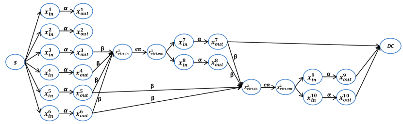
Figure 1: Example of an information flow graph: $k=3,d=4,n=6,e=2$. The unlabeled edges have capacity $\infty$. Nodes 1 and 2 are repaired in the first stage and nodes 3 and 4 are repaired in the second stage. A data collector connecting to any 3 nodes should be able to recover the entire information.

II-C Network coding analysis

The key idea behind representing the repair problem by an IFG lies in the observation that the repair problem can be cast as a multicast network coding problem [4]. Celebrated results from network coding [5, 6] are then invoked to establish the fundamental limits of the repair problem.

According to the max-flow bound of network coding[5], for a data collector to be able to reconstruct the data, the min-cut separating the source to the data collector should be larger or equal to the data object size $\mathcal{M}$. Considering all possible data collectors and all possible failure patterns, and assuming that the number of failures/repairs is bounded, the following condition is necessary and sufficient for the existence of centralized multi-node repair codes [4, Proposition 1]

$$\min\limits_{G\in\mathcal{G}}\min\limits_{t\in\text{DC}(G)}\text{mincut}_{G}(s,t)\geq\mathcal{M}.$$ (2)

Analyzing the minimum cut of all IFGs result in the following theorem.

Theorem 1.

For fixed system parameters $(\mathcal{M},n,k,d,e,\alpha,\beta)$, assuming that the number of failures/repairs is bounded, regenerating codes satisfying the centralized multi-node repair condition exist if and only if

$$\mathcal{M}\leq\min\limits_{\mathbf{u}\in\mathcal{P}}\left(\sum\limits_{i=1}^{g}\min(u_{i}\alpha,(d-\sum\limits_{j=1}^{i-1}u_{j})\beta)\right)\triangleq\min\limits_{\mathbf{u}\in\mathcal{P}}f(\mathbf{u}),$$ (3)

where

$$f(\mathbf{u})=\sum\limits_{i=1}^{g}\min(u_{i}\alpha,(d-\sum\limits_{j=1}^{i-1}u_{j})\beta),$$ (4)

$$\mathcal{P}=\{\mathbf{u}=[u_{1},\ldots,u_{g}]:1\leq u_{i}\leq e,g\in\mathbb{N}\text{ such that }\sum\limits_{i=1}^{g}u_{i}=k\}.$$ (5)

Note that $g$ in (5) corresponds to the support of $\mathbf{u}$, and it satisfies $\lceil\frac{k}{e}\rceil\leq g\leq k$. We call the vector $\mathbf{u}\in\mathcal{P}$ a recovery scenario.

Proof:

Consider the scenario $\mathbf{u}\in\mathcal{P}$ as follows. A data collector DC connects to a subset of $k$ nodes $\{x_{out}^{j}:j\in I\}$, where $I$ is the set of $k$ contacted nodes. The size of the support of $\mathbf{u}$ corresponds to the number of repair groups of size $e$ taking part in the reconstruction process, while $u_{i}$ corresponds to the number of nodes contacted from repair group $i$.

As all incoming edges of DC have infinite capacity, we only examine cuts $(U,\bar{U})$ with $S\in U$ and $\{x_{out}^{i}:i\in I\}\subseteq\bar{U}$. Every directed acyclic graph has a topological sorting, which is an ordering “$<$” of its vertices such that the existence of an edge $x\to y$ implies $x<y$. We recall that nodes within the same repair group are repaired simultaneously, hence it is possible that all input (or output) nodes in a repair group are adjacent in the the ordering. We thus order the $g$ repair groups connected to DC according to the sorting. Since nodes are sorted, nodes in the $i$-th repair group do not have incoming edges from nodes in the $j$-th repair group, with $j>i,i,j\in[g]$.

Considering the $i$-th repair group, consider the case $|\left\{x_{\text{in}}^{i}\in U\right\}|=m$ and the remaining nodes are such that $x_{\text{in}}^{i}\in\bar{U}$.

• if $x_{\text{in}}^{i}\in U$, then the contribution of each node is $\alpha$. The overall contribution of these nodes is $m\alpha$.

• else: $x_{\text{in}}^{i}\in\bar{U}$, then if $x_{\text{virt,out}}^{i}\in U$, the contribution of this node is $\infty$. Thus, we only consider the case $x_{\text{virt,out}}^{i}\in\bar{U}$. Then, we discuss two cases

  • if $x_{\text{virt,in}}^{i}\in U$, the contribution to the cut is $e\alpha$.

  • else, since the $i$-th group is the topologically i-th repair group, at most $\sum\limits_{j=1}^{i-1}u_{j}$ edges come from output nodes in $\bar{U}$. The contribution is $(d-\sum\limits_{j=1}^{i-1}u_{j})\beta$. Thus, the contribution of this node is $\min(e\alpha,(d-\sum\limits_{j=1}^{i-1}u_{j})\beta)$. Note that $x_{\text{virt,out}}^{i}\in\bar{U}$, we do not need to account for other similar nodes.

Hence, if $m=u_{i}$, the contribution of the i-th repair group is $u_{i}\alpha$. If $m<u_{i}$, the contribution is $m\alpha+\min(e\alpha,(d-\sum\limits_{j=1}^{i-1}u_{j})\beta)$, which is minimized to be $\min(e\alpha,(d-\sum\limits_{j=1}^{i-1}u_{j})\beta)$ when $m=0$. Thus, to lower the cut, either $m=u_{i}$ in the case of $(d-\sum\limits_{j=1}^{i-1}u_{j})\beta>u_{i}\alpha$ or $m=0$ otherwise. The total contribution of the $i$-th repair group is then

$$\min(u_{i}\alpha,(d-\sum\limits_{j=1}^{i-1}u_{j})\beta).$$

Finally, summing all contributions from different repair groups and considering the worst case for $\mathbf{u}\in\mathcal{P}$ implies that

$$\min\limits_{G\in\mathcal{G}}\min\limits_{t\in\text{DC}(G)}\text{mincut}_{G}(s,t)=\min\limits_{\mathbf{u}\in\mathcal{P}}\left(\sum\limits_{i=1}^{g}\min(u_{i}\alpha,(d-\sum\limits_{j=1}^{i-1}u_{j})\beta)\right),$$

with $\mathcal{P}$ defined as in (5). The theorem follows according to the necessary and sufficient condition in (2). ∎

Our characterization of Theorem 1 relies on the boundedness assumption of the total number of failures/repairs. A future direction is to investigate the correctness of Theorem 1 for arbitrary number of failures/repairs, similar to [26, 44].

II-D Solving the minimum cut problem

In this section, we derive the structure of the optimal scenario $\mathbf{u}$ in (3) for any set of parameters $(\alpha,\beta)$. For instance, we show that for $me<k\leq(m+1)e$, the number of optimal repair groups $g^{*}$ (the support of $\mathbf{u}$) is equal to $m+1$. The result is formalized in the following theorem. Recall that we denote $\eta=\lfloor k/e\rfloor,r=k-\eta e$.

Theorem 2.

For fixed system parameters $(\mathcal{M},n,k,d,e,\alpha,\beta)$, functional regenerating codes satisfying the centralized multi-node repair condition exist if and only if

$$\mathcal{M}\leq f(\mathbf{u^{*}})=\sum\limits_{i=1}^{\lceil\frac{k}{e}\rceil}\min(u^{*}_{i}\alpha,(d-\sum\limits_{j=1}^{i-1}u^{*}_{j})\beta),$$ (6)

where

$$\mathbf{u}^{*}=\begin{cases}[k],&\text{if }k\leq e,\\ [\underbrace{e,\ldots,e}_{\eta\text{ times}}],&\text{else if }k=\eta e,\\ [r,\underbrace{e,\ldots,e}_{\eta\text{ times}}],&\text{else if }k=\eta e+r\text{ and }\alpha\leq\frac{d+\eta r-\eta e}{r}\beta,\\ [\underbrace{e,\ldots,e}_{\eta\text{ times}},r],&\text{otherwise},\\ \end{cases}$$ (7)

where $0<r<e$.

Note that $[k]$ in (7) means a vector with a single entry $k$. We note that [23, 24] have independently developed Theorem 1 or an equivalent of Theorem 1, without entirely characterizing the optimal solution. [45] independently proved via a different approach Theorem 2, except for the last case in (7).

We denote by $[\mathbf{v},\mathbf{u},\mathbf{w}]$ the vector that is the concatenation of the vectors $\mathbf{v},\mathbf{u},\mathbf{w}$. The next lemma shows that the minimum cut can be obtained by optimizing any subsequence of $\mathbf{u}$ first. The proof follows directly from the definition of $f()$ in (4) and is omitted.

Lemma 1.

Consider vectors $\mathbf{v},\mathbf{w},\mathbf{u},\mathbf{u^{\prime}}$ such that $\sum_{i}u_{i}=\sum_{i}u^{\prime}_{i}$. If

$$f(\mathbf{u})\geq f(\mathbf{u^{\prime}}),$$ (8)

then,

$$f([\mathbf{v},\mathbf{u},\mathbf{w}])\geq f([\mathbf{v},\mathbf{u}^{\prime},\mathbf{w}]).$$ (9)

In proving the result of Theorem 2, we first characterize the optimal solution in the case of $k\leq e$. Insight and intuition gained from this case are used to motivate and derive the general optimal solution. We first state the following lemma, which represents a key step towards proving our result.

Lemma 2.

Let $\alpha,\beta$ be non-negative reals, $u_{1},u_{2},d,e,s,l$ be non-negative integers such that $u_{1}+u_{2}=s\leq e$, then the following inequality holds

$$f([u_{1},\underbrace{e,\ldots,e}_{l\text{ times}},u_{2}])\geq\min(f([s,\underbrace{e,\ldots,e}_{l\text{ times}}]),f([\underbrace{e,\ldots,e}_{l\text{ times}},s])),$$ (10)

where $f(\mathbf{u})$ is defined as in (4).

Proof:

To prove the result, we cast it as an optimization problem:

$$\underset{\mathbf{u}=[u_{1},u_{2}]}{\text{minimize}}\qquad\min(u_{1}\alpha,d\beta)+\sum\limits_{i=0}^{l-1}\min(e\alpha,(d-ie-u_{1})\beta)+\min(u_{2}\alpha,(d-(l+1)e-u_{1})\beta)$$

$$\text{subject to}\qquad 0\leq u_{1}\leq s,$$

$$\qquad\qquad\qquad 0\leq u_{2}\leq e,$$

$$\qquad\qquad\qquad u_{1}+u_{2}=s.$$ (11)

Substituting $u_{2}$ by $s-u_{1}$ in (11), using the identity $\min(x,y)=\frac{x+y-|x-y|}{2}$ and after eliminating constant terms, (11) becomes equivalent to

$$\underset{u_{1}}{\text{minimize}}-u_{1}l\beta-|u_{1}\alpha-d\beta|-\sum\limits_{i=0}^{l-1}|e\alpha-d\beta+ie\beta+u_{1}\beta|-|s\alpha-u_{1}(\alpha-\beta)-(d-le)\beta|$$

$$\text{subject to}\qquad 0\leq u_{1}\leq s.$$ (12)

The objective function in (12), as a function of $u_{1}$, is concave over the interval $[0,s]$. The concavity is due to the convexity of $x\to|x|$. Therefore, the minimum is achieved at one of the extreme values. Equivalently, $u_{1}^{*}=s$ or $u_{1}^{*}=0$. ∎

II-D1 Case $k\leq e$

In this scenario, connecting to $k$ nodes from the same repair group yields the worst case scenario from an information flow perspective. Given a particular repair scenario characterized by a vector $\mathbf{u}$, for any two adjacent repair groups (i.e., two adjacent entries in $\mathbf{u}$) with $u_{1}$ and $u_{2}$ nodes respectively, we have $u_{1}+u_{2}\leq e$. One can combine these two groups into a single repair group to achieve a lower cut value. Indeed, from the cut expression in (3), the contribution of the initial set $[u_{1},u_{2}]$ to the cut is $\min(u_{1}\alpha,l\beta)+\min(u_{2}\alpha,(l-u_{1})\beta),$ for some non-negative integer $l$. After combining the groups into a single repair group, the contribution of the newly formed repair group is $\min((u_{1}+u_{2})\alpha,l\beta)$, which is lower than the initial contribution by virtue of Lemma 2, thus achieving a lower cut. This means that starting from an IFG, we construct a new IFG that has one less repair group and lower min-cut value. This process can be repeated until we end up with a single repair group consisting of $k\leq e$ nodes, which corresponds to the minimum cut over all graphs in this case.

Therefore, the tradeoff in (3) is simply characterized by $\mathcal{M}\leq\min(k\alpha,d\beta)$. Moreover, $\alpha_{\text{MSMR}}=\alpha_{\text{MBMR}}=\frac{\mathcal{M}}{k}$ and $\beta_{\text{MSMR}}=\beta_{\text{MBMR}}=\frac{\mathcal{M}}{d}$. Equivalently, the functional storage bandwidth tradeoff reduces to a single point given by $(\alpha_{\text{MSMR}},\beta_{\text{MSMR}})=(\alpha_{\text{MBMR}},\beta_{\text{MBMR}})=(\frac{\mathcal{M}}{k},\frac{\mathcal{M}}{d})$.

II-D2 Case $e<k$

Motivated by the previous case, the intuition is that, given a scenario $\mathbf{u}$, one should form a new scenario which exhibits as many groups of size $e$ as possible. Subsequently, one constructs a scenario $\mathbf{u}$ such that all its entries, except maybe one entry, are equal to $e$. Lemma 2 addresses the case $u_{1}+u_{2}\leq e$. Generalizing it to the case where $e\leq u_{1}+u_{2}\leq 2e$ follows the same approach.

Lemma 3.

Let $\alpha,\beta$ be non-negative reals, $u_{1},u_{2},d,e,s,l$ be non-negative integers such that $u_{1}+u_{2}=e+s$ and $0\leq u_{1},u_{2},s\leq e$. Then, the following inequality holds

$$f([u_{1},\underbrace{e,\ldots,e}_{l\text{ times}},u_{2}])\geq\min(f([s,\underbrace{e,\ldots,e}_{l+1\text{ times}}]),f([\underbrace{e,\ldots,e}_{l+1\text{ times}},s])),$$ (13)

where $f(\mathbf{u})$ is defined as in (4).

Proof:

First, we notice that $u_{1}=e+s-u_{2}\geq s$ as $u_{2}\leq e$. Then, the proof follows along similar lines as that of Lemma 2 by replacing the constraint in (12) by $s\leq u_{1}\leq e$. ∎

For a fixed $\beta$, we denote the cut corresponding to $\mathbf{u}=[\underbrace{e,\ldots,e}_{j\text{times}},r,\underbrace{e,\ldots,e}_{\eta-j\text{ times}}]$, as a function of $\alpha$, by $C_{j}(\alpha),j=0,\ldots,\eta$. As will be shown later in the proof of Theorem 2, a careful analysis of the behavior of the $\eta+1$ different scenarios $C_{j}(\alpha),0\leq j\leq\eta,$ is needed to determine the overall optimal scenario. We state the result in the following lemma, whose proof is relegated to Appendix -A.

Lemma 4.

Assume $e\nmid k$. There exists a real number $\alpha_{c}(\eta)\in[\frac{d}{e}\beta,\frac{d}{r}\beta]$ such that, for any $0\leq j\leq\eta$,

$$C_{j}(\alpha)\begin{cases}\geq C_{0}(\alpha),&\text{if }\alpha\leq\alpha_{c}(\eta),\\ \geq C_{\eta}(\alpha),&\text{if }\alpha\geq\alpha_{c}(\eta),\end{cases}$$ (14)

with

$$\alpha_{c}(\eta)=\frac{d+\eta r-\eta e}{r}\beta.$$ (15)

Proof:

Now that we have the necessary machinery, we proceed as follows: given any scenario $\mathbf{u}$, we keep combining and/or changing repair groups by means of successive applications of Lemma 2 and Lemma 3 on subsequences of $\mathbf{u}$ until we can no longer reduce the minimum cut. By Lemma 1 we reduced the overall minimum cut. The algorithm terminates because at each step, either the number of repair groups in $\mathbf{u}$ is reduced by one, or the number of repair groups of full size $e$ is increased by one. As the number of repair groups is lower bounded by $\eta+1$, and as the number of repair groups of full size $e$ is upper bounded by $\eta$, the algorithm must terminate after a finite number of steps. It can be seen then that the above reduction procedure has a finite number of outcomes, given by

• $\mathbf{u}=[\underbrace{e,\ldots,e}_{\eta\text{ times}}]$ if $k=\eta e$,

• $\mathbf{u}=[\underbrace{e,\ldots,e}_{j\text{times}},r,\underbrace{e,\ldots,e}_{\eta-j\text{ times}}]$ when $k=\eta e+r$,
  with $0<r<e$ and $j\in\{0,\ldots,\eta\}$.

Therefore, if $e\mid k$, then the optimal scenario corresponds to considering exactly $\eta$ repair groups. On the other hand, if $e\nmid k$, then, it is optimal to consider exactly $\eta+1$ repair groups. However, the optimal position of the repair group with $r$ nodes needs to be determined. Then, using Lemma 4, the result in Theorem 2 follows. ∎

Example 1.

Let $\mathbf{u}=[1,3,2,3,2]$ with $e=3$. Then, one can start by reducing the first three repair groups $[1,3,2]$. This leads to $\mathbf{u}=[3,3,3,2]$. Another approach would be to consider the last three repair groups $[2,3,2]$. Reducing this vector leads to either $\mathbf{u}=[1,3,3,3,1]$ or $\mathbf{u}=[1,3,1,3,3]$. Reducing further $\mathbf{u}=[1,3,3,3,1]$ leads to $\mathbf{u}=[2,3,3,3]$ or $\mathbf{u}=[3,3,3,2]$. Reducing $\mathbf{u}=[1,3,1,3,3]$ leads to $\mathbf{u}=[3,2,3,3]$ or $\mathbf{u}=[2,3,3,3]$. It remains to compare the cuts given by $\mathbf{u}=[3,3,3,2]$, $\mathbf{u}=[3,3,2,3]$, $\mathbf{u}=[3,2,3,3]$ and $\mathbf{u}=[2,3,3,3]$. Following Theorem 2, either $\mathbf{u}=[2,3,3,3]$ or $\mathbf{u}=[3,3,3,2]$ gives the lowest min-cut.

II-E Explicit expression of the tradeoff

Having characterized the optimal scenario generating the minimum cut in the last section, we are now ready to state the admissible storage-repair bandwidth region for the centralized multi-node repair problem, the proof of which is in Appendix -B.

Theorem 3.

For an $(\mathcal{M},n,k,d,e,\alpha,\beta)$ storage system, there exists a threshold function $\alpha^{*}(\mathcal{M},n,k,d,e,\gamma)$ such that for any $\alpha\geq\alpha^{*}(\mathcal{M},n,k,d,e,\gamma)$, regenerating codes exist. For any $\alpha<\alpha^{*}(\mathcal{M},n,k,d,e,\gamma)$, it is impossible to construct codes achieving the target parameters. The threshold function $\alpha^{*}(\mathcal{M},n,k,d,e,\gamma)$ is defined as follows:
$\bullet$ if $k\leq e$, then: $\alpha^{*}=\frac{\mathcal{M}}{k},\ \gamma\in[\mathcal{M},+\infty)$,
$\bullet$ if $k=\eta e,\eta\geq 2$, then:

$$\alpha^{*}=\begin{cases}\frac{\mathcal{M}}{k},&\gamma\in[f_{0}(\eta-1),+\infty),\\ \frac{\mathcal{M}-\gamma g_{0}(i)}{ie},&\gamma\in[f_{0}(i-1),f_{0}(i)],i=\eta-1,\ldots 1,\end{cases}$$ (16)

$\bullet$ if $k=\eta e+r$ with $\eta\geq 1,1\leq r\leq e-1$, then:

$$\alpha^{*}=\begin{cases}\frac{\mathcal{M}}{k},&\gamma\in[f_{r}(\eta-1),+\infty),\\ \frac{\mathcal{M}-\gamma g_{r}(i)}{r+ie},&\gamma\in[f_{r}(i-1),f_{r}(i)],i=\eta-1,\ldots 1,\\ \frac{\mathcal{M}-\gamma g_{r}(0)}{r},&\gamma\in[\frac{d\mathcal{M}}{(\eta+1)d-e{\eta+1\choose 2}},f_{r}(0)],\end{cases}$$ (17)

where

$$f_{r}(i) =\frac{2ed\mathcal{M}}{-k^{2}-r^{2}+e(k-r)+2kd-e^{2}(i^{2}+i)-2ier},$$ (18)

$$g_{r}(i) =\frac{(\eta-i)(-2r+e+2d-\eta e-ei)}{2d}.$$ (19)

The functional repair tradeoff is illustrated in Figure 2 for multiple values of $e\in\{1,2,3,4,8\}$ and $k=8,d=10,$ $\mathcal{M}=1$.

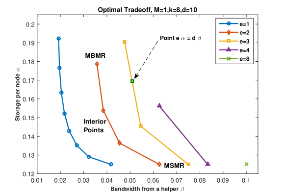
Figure 2: Multi-node repair tradeoff: $k=8,d=10,\mathcal{M}=1,e\in\{1,2,3,4,8\}$. When $e\nmid k$, the point with $e\alpha=d\beta$ is not the MBMR point.

Remark 1.

In the case of $e|k,e|d$, the following equality holds for all points on the tradeoff

$$\mathcal{M} =\sum\limits_{i=0}^{\eta-1}\min(e\alpha,(d-ie)\beta)\iff\frac{\mathcal{M}}{e}=\sum\limits_{i=0}^{\eta-1}\min(\alpha,(\frac{d}{e}-i)\beta).$$

Therefore, the tradeoff between $\alpha$ and $\beta$ is the same as the single erasure tradeoff of a system with reduced parameters given by $\frac{\mathcal{M}}{e}$, $\frac{k}{e}=\eta$ and $\frac{d}{e}$. The expression of the tradeoff in this case can be recovered from [4] with the appropriate parameters.

We now have the expressions of the two extreme points on the optimal tradeoff. We focus on the case $e<k$, as otherwise the optimal tradeoff reduces to a single point.

MSMR. The MSMR point is the same irrespective of the relation between $k$ and $e$, and it is given by

$$\alpha_{\text{MSMR}}=\frac{\mathcal{M}}{k},\gamma_{\text{MSMR}}=\frac{\mathcal{M}}{k}\frac{ed}{d-k+e}.$$ (20)

MBMR. Interestingly, the MBMR point depends on whether $e$ divides $k$ or not.

$\bullet$ If $k=\eta e$, we obtain

$$\gamma_{\text{MBMR}} =\frac{2ed\mathcal{M}}{-k^{2}+ek+2kd}=\frac{d\mathcal{M}}{d\eta-e\binom{\eta}{2}},$$ (21)

$$\alpha_{\text{MBMR}} =\frac{\gamma_{\text{MBMR}}}{e}.$$ (22)

The amount of information downloaded for repair is equal to the amount of information stored at the $e$ replacement nodes. This property of the MBMR point is similar to the minimum bandwidth point in the single erasure case [4] and also the minimum bandwidth cooperative repair point [26].

$\bullet$ If $k=\eta e+r$, we obtain

$$\gamma_{\text{MBMR}} =\frac{2ed\mathcal{M}}{(k-r+e)(2d-k+r)}=\frac{d\mathcal{M}}{d(\eta+1)-e\binom{\eta+1}{2}},$$ (23)

$$\alpha_{\text{MBMR}} =\gamma_{\text{MBMR}}\frac{d+\eta r-e\eta}{rd}.$$ (24)

This situation is novel for multiple erasures as the $e$ nodes need to store more than the overall downloaded information. This is an extra cost in order to achieve the low value of the repair bandwidth. Figure 2 illustrates this situation with $e=3,k=8$. However, later we will see that for both $e|k$ and $e\nmid k$, the total bandwidth at MBMR is equal to the entropy of the failed nodes (see Lemma 6 and Lemma 11):

$$H(W_{E})=d\beta=\gamma,$$ (25)

where $E\subset[n]$ is any subset of nodes of size $e$ and $W_{E}$ is the information stored across the nodes in $E$.

Remark 2.

From the statement of Theorem 2, we note that if we only consider points between the MSMR and the MBMR points, then the scenario $\mathbf{u}=[r,e,\dots,e]$ always generates the lowest cut. In fact, the scenario $\mathbf{u}=[e,\dots,e,r]$ corresponds to points beyond the MBMR point, namely, points with $\alpha\geq\alpha_{\text{MBMR}},\beta=\beta_{\text{MBMR}}$.

Remark 3.

We compare the centralized repair scheme repairing $e$ nodes to a separate strategy repairing each of the $e$ nodes separately using single erasure regenerating codes. We fix $k,\alpha$ and $\mathcal{M}$.
Case I: both strategies use $d$ helpers. The separate strategy requires a total bandwidth given by $ed\beta_{1}$, while the centralized repair requires $d\beta_{e}$, where the subscript indicates the number of erasures repaired at a time. For simplicity, we assume that $e\mid k$. The case $e\nmid k$ can be treated in a similar way. For points on the multi-node repair tradeoff, we have

$$\mathcal{M}=\sum\limits_{j=0}^{\eta-1}\min(e\alpha,(d-je)\beta_{e}).$$

Consider a point with the same $\alpha$ and $d$ on the single erasure tradeoff, we write

$$\mathcal{M}=\sum\limits_{j=0}^{\eta-1}\min(e\alpha,(d-je)\beta_{e})=\sum\limits_{j=0}^{k-1}\min(\alpha,(d-j)\beta_{1})=\sum\limits_{j=0}^{\eta-1}\sum\limits_{i=0}^{e-1}\min(\alpha,(d-i-je)\beta_{1}) \leq\sum\limits_{j=0}^{\eta-1}e\min(\alpha,(d-je)\beta_{1})$$

$$=\sum\limits_{j=0}^{\eta-1}\min(e\alpha,(d-je)e\beta_{1}).$$

It follows that $\beta_{e}\leq e\beta_{1}$ with equality if and only if $e=1$. Therefore, for any storage capacity $\alpha$, multi-node repair requires strictly less bandwidth than a separate strategy for the same number of helpers $d$.
Case II: multi-node repair uses $d-e+1$ helpers, and separate repair uses $d$ helpers. In this case, the original number of available nodes that can serve as helpers is assumed to be $d$, and $e\geq 1$ erasures occur within the available nodes. Then a separate strategy may require a smaller bandwidth for some values of $\alpha$, as illustrated by Figure 3. However, as $d$ is sufficiently large, we observe numerically that multi-node repair with $d-e+1$ helpers performs better than a separate strategy for all values of $\alpha$. Moreover, for the MSMR point, the separate repair bandwidth is $ed\beta_{1,\text{MSR}}=e\frac{\mathcal{M}}{k}\frac{d}{d-k+1}$, and centralized repair bandwidth is $(d-e+1)\beta_{e,\text{MSMR}}=\frac{\mathcal{M}}{k}\frac{e(d-e+1)}{d-k+1}$. It follows that a centralized repair is always better that a lazy repair strategy, specifically, for $e>2$,

$$\frac{(d-e+1)\beta_{e,\text{MSMR}}}{ed\beta_{1,\text{MSR}}}=\frac{d-(e-1)}{d}<1.$$ (26)

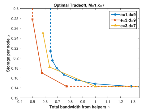
Figure 3: Centralized multi-node repair vs separate repair strategy: $k=7,\mathcal{M}=1$. Separate repair strategy uses $d=9$ to repair 3 nodes successively while multi-node repair is plotted for $d=7$ and $d=9$.

III Exact-repair MSMR codes constructions

In the remainder of the paper, we study exact repair. In this section, we first analyze the case $e\geq k$ and then construct MSMR codes when $e<k$. In later sections, we study the feasibility of MBMR codes and the interior points under exact repair for $e<k$.

III-A Construction when $k\leq e$

In the case of $k\leq e$, the optimal tradeoff reduces to a single point, so our MSMR construction in this section is also an MBMR code. The optimal parameters satisfy $\alpha=\frac{\mathcal{M}}{k},\beta=\frac{\mathcal{M}}{d}$ and $\gamma=\mathcal{M}$. We note that the overall repair bandwidth $d\beta$ and the reconstruction bandwidth $k\alpha$ are the same. Therefore, one can achieve $\alpha$ and $\gamma$ by dividing the data into $k$ symbols and encoding them using an $(n,k)$ MDS code (for example, a Reed-Solomon code). The repair can be done by downloading the full content of any $k$ out of $d$ helpers while not using $d-k$ helpers. Such repair is asymmetric in nature. We describe one alternative approach for achieving the repair with equal contribution from $d$ helpers.

1. Divide the original file into $kd$ symbols (that is $\mathcal{M}=kd$) and encode them using an $(nd,kd)$ MDS code.

2. Store the encoded symbols at $n$ nodes, such that each node stores $\alpha=d$ encoded symbols.

3. For reconstruction, from any $k$ nodes, we obtain $kd$ different symbols. By virtue of the MDS property, we can reconstruct the data.

4. For repair, each helper node transmits any $\beta=\frac{\mathcal{M}}{d}=k$ symbols. The replacement nodes receive $dk$ different coded symbols, which are sufficient to reconstruct the whole data and thus regenerate the missing symbols.

Remark 4.

The above procedure works for a specific predetermined $d$. However, it can be generalized to support any value of $d$ satisfying $k\leq d\leq n-e$. For instance, let $\delta=\text{lcm}(k,k+1,k+2,\ldots,n-e)$ (lcm denotes the least common multiple). Assume $\mathcal{M}=k\delta$. The file of size $\mathcal{M}$ is then encoded using an $(n\delta,k\delta)$ MDS code. Each node stores $\alpha=\frac{\mathcal{M}}{k}=\frac{k\delta}{k}=\delta$ coded symbols. For repair with $d$ helpers, for any $k\leq d\leq n-e$, each node transmits any $\beta=\frac{\mathcal{M}}{d}=\frac{k\delta}{d}$ coded symbols for his node. Similarly, it can be seen that reconstruction is always feasible.

III-B Minimum storage codes framework

In the following subsections, we discuss an explicit MSMR code construction method using existing MSR codes designed for single failures for $k>e$. We first describe the general framework, and then present two specific codes.

The framework described in this section has been developed in [36] for numerical simulations. We present it here in a formal and analytical way. Consider an instance of an exact linear $(n,k,d,\alpha,\beta)$ MSR code, where $\beta=\frac{\alpha}{d-k+1}$. Consider $e$ nodes, indexed by $f_{1},\ldots,f_{e}$, and other distinct $d-e+1$ nodes, indexed by $h_{1},\ldots,h_{{d-e+1}}$, such that $d-e+1\geq k$. Let $\mathcal{H}=\{f_{1},\ldots,f_{e},h_{1},\ldots,h_{{d-e+1}}\}$ and define $\mathcal{H}_{f_{j}}=\mathcal{H}\backslash\{f_{j}\}$. Consider the single-node repair algorithm corresponding to failed node $f_{j}$ and helper nodes $\mathcal{H}_{f_{j}}$. We denote by $\mathbf{s}_{h,f_{j}}^{\mathcal{H}}$ the information sent by node $h$ to repair node $f_{j}$, for helpers $h\in\mathcal{H}_{f_{j}}$. We drop the superscript $\mathcal{H}$ when it is clear from the context. The size of $\mathbf{s}_{h,f_{j}}$ is $\beta$ symbols.

Now we construct an $(n,k,d-e+1,e,\alpha,e\beta)$ MSMR code. Upon failure of the $e$ nodes $f_{1},\ldots,f_{e}$, the centralized node carrying the repair connects to the set of $d-e+1$ helpers $h_{1},\ldots,h_{{d-e+1}}$. Each helper node $h_{i}$ transmits $e\beta$ symbols given by $\cup_{j=1}^{e}\{\mathbf{s}_{h_{i},f_{j}}\}.$ One can check that the parameters of an MSMR code in (20) are satisfied with equality.

The approach consists in using the underlying MSR repair procedure for each of the $e$ failed nodes. Note that $\mathbf{s}_{h_{i},f_{j}}$ can be obtained from the $d-e+1$ helpers, for $i\in[d-e+1]$. To this end, the MSR repair procedure requires $\mathbf{s}_{f_{i},f_{j}}^{\mathcal{H}}$ for all $\{(i,j):i,j\in[e],i\neq j\}$, which we treat as unknowns. Let ${E}_{i,j}(\cdot)$ denote the encoding function used to encode the information sent from node $h_{i}$ to node $f_{j}$. Also, let ${D}_{i}(\cdot)$ denote the decoding function used by the MSR code to repair node $f_{i}$ given information from $d$ helpers. Then, we write

$$\mathbf{s}_{f_{i},f_{j}}^{\mathcal{H}} ={E}_{i,j}(\mathbf{w}_{f_{i}})$$

$$={E}_{i,j}({D}_{i}(\mathbf{s}_{h,f_{i}}^{\mathcal{H}},h\in\mathcal{H}_{f_{i}})),$$ (27)

where $\mathbf{w}_{j}$ denotes the content of node $j$, $i,j\in[e],i\neq j$. Equation (27) generates $e(e-1)\beta$ linear equations in $e(e-1)\beta$ unknowns. Let $\mathbf{s}$ be a vector containing the unknowns $\mathbf{s}_{f_{i},f_{j}}$. Then, we seek to form a system of linear equations as

$$A\mathbf{s}=\mathbf{b},$$ (28)

where $A$ is a known $(e(e-1)\beta\times e(e-1)\beta)$ matrix and $b$ is a known $(e(e-1)\beta\times 1)$ vector. If $A$ is non-singular, one can thus recover $\mathbf{s}$. Then, the centralized node can recover the failed node $\mathbf{w}_{f_{i}}$ as $\mathbf{w}_{f_{i}}={D}_{i}(\mathbf{s}_{h,f_{i}},h\in\mathcal{H}_{f_{i}})$. We adopt the above framework throughout the section.

Remark 5.

While the described framework applies to codes with arbitrary rates, we focus in the sequel on low-rate codes. High-rate MSMR constructions have been presented in [35]. However, in the low-rate regime, our constructions perform better. For instance, for a target MSMR code with rate $\frac{1}{2}$, the construction in [35] yields a storage size $\alpha=k^{2k-1}$, while applying the above approach to IA codes [8] or to PM codes [43] results in a smaller storage size $\alpha=k$ and $\alpha=k-1$, respectively.

III-C Product-matrix codes

In this subsection, we construct MSMR codes for any $e$ erasures based on product-matrix (PM) codes [43]. The PM framework allows the design of MBR codes for any value of $d$ and the design of MSR codes for $d\geq 2k-2$. Moreover, the PM construction offers simple encoding and decoding and ensures optimal repair of all nodes. Product-matrix MSR codes are a family of scalar MSR codes, i.e., $\beta=1$. We first focus on the case $d=2k-2$. Under this setup, $\alpha=d-k+1=k-1$. The codeword is represented by an $(n\times\alpha)$ code matrix $C$ such that its $i^{\text{th}}$ row corresponds to the $\alpha$ symbols stored by the $i^{\text{th}}$ node. The code matrix is given by

$$C=\Psi M,\Psi=\begin{bmatrix}\Phi&\Lambda\Phi\end{bmatrix},M=\begin{bmatrix}S_{1}\\ S_{2}\end{bmatrix},$$ (29)

where $\Psi$ is an $(n\times d)$ encoding matrix and $M$ is a $(d\times\alpha)$ message matrix. $S_{1}$ and $S_{2}$ are $(\alpha\times\alpha)$ symmetric matrices constructed such that the ${\alpha+1\choose 2}$ entries in the upper-triangular part of each of the two matrices are filled up by ${\alpha+1\choose 2}$ distinct message symbols. $\Phi$ is an $(n\times\alpha)$ matrix and $\Lambda$ is an $(n\times n)$ diagonal matrix. The elements of $\Psi$ should satisfy:

1. any $d$ rows of $\Psi$ are linearly independent;

2. any $\alpha$ rows of $\Phi$ are linearly independent;

3. the $n$ diagonal elements of $\Lambda$ are distinct.

The above conditions may be met by choosing $\Psi$ to be a Vandermonde matrix, in which case its $i^{\text{th}}$ row is given by $\mathbf{\psi}_{i}^{t}=\begin{bmatrix}1&\lambda_{i}&\cdots&\lambda_{i}^{d-1}\end{bmatrix}$. It follows that $\Lambda=\text{diag}\{\lambda_{1}^{\alpha},\ldots,\lambda_{n}^{\alpha}\}$. In the following, we assume that $\Psi$ is a Vandermonde matrix.

Repair of a single erasure in PM codes. The single erasure repair algorithm [43] is reviewed below. Let $\mathbf{w}_{i}^{t}$ denote the content stored at a failed node. Let $\mathbf{\phi}_{i}^{t}$ be the $i^{\text{th}}$ row of $\Phi$. Then, $\mathbf{w}_{i}^{t}=\mathbf{\psi}_{i}^{t}M=\begin{bmatrix}\mathbf{\phi}_{i}^{t}&\lambda_{i}^{\alpha}\mathbf{\phi}_{i}^{t}\end{bmatrix}M=\mathbf{\phi}_{i}^{t}S_{1}+\lambda_{i}^{\alpha}\mathbf{\phi}_{i}^{t}S_{2}$. Let $\mathcal{H}_{i}=\{h_{1},\ldots,h_{d}\}$ denote the set of $d$ helpers. Each helper $h$ transmits $s_{h,i}=\mathbf{w}_{h}^{t}\mathbf{\phi}_{i}=\mathbf{\psi}^{t}_{h}M\mathbf{\phi}_{i}$ to the replacement node, who obtains $\Psi_{\mathcal{H}_{i}}M\mathbf{\phi}_{i}$, where $\Psi_{\mathcal{H}_{i}}^{t}=\begin{bmatrix}\mathbf{\psi}_{h_{1}}&\cdots&\mathbf{\psi}_{h_{d}}\end{bmatrix}.$ Note that $\Psi_{\mathcal{H}_{i}}$ is invertible by construction. Thus, using the symmetry of $S_{1}$ and $S_{2}$, we obtain $(M\mathbf{\phi}_{i})^{t}=\begin{bmatrix}\mathbf{\phi}_{i}^{t}S_{1}&\mathbf{\phi}_{i}^{t}S_{2}\end{bmatrix}$. We can then reconstruct $\mathbf{w}_{i}^{t}=\mathbf{\phi}_{i}^{t}S_{1}+\lambda_{i}^{\alpha}\mathbf{\phi}_{i}^{t}S_{2}$.

Repair of multiple erasures in PM codes. Given the symmetry of PM codes, we can assume w.l.o.g that nodes in $\mathcal{E}=\{1,\ldots,e\}$ have failed. Define $\mathcal{E}_{i}=\mathcal{E}\backslash\{i\}$. Let $\mathcal{H}=\{1,\ldots,d+1\}$. The centralized node connects to helper node $h\in\{e+1,\ldots,d+1\}$, and obtains $\{\mathbf{\psi}_{h}^{t}M\mathbf{\phi}_{j},j\in\mathcal{E}\}$.

Let $\mathbf{s}=[s_{1,2},s_{2,1},\ldots,s_{1,e},s_{e,1},\ldots,s_{e-1,e},s_{e,e-1}]^{t}$. Our goal is to express explicitly $A$ and $\mathbf{b}$ as in (28).

Consider the repair of node $i\in\mathcal{E}$ by the set of helpers in $\mathcal{H}_{i}=\mathcal{H}\backslash\{i\}$. From the previous subsection, we write

$$\mathbf{w}_{i} =\begin{bmatrix}I_{\alpha}&\lambda^{\alpha}_{i}I_{\alpha}\end{bmatrix}\Psi_{\mathcal{H}_{i}}^{-1}\mathbf{s}_{\mathcal{H}_{i}},\text{ such that }$$ (30)

$$\Psi_{\mathcal{H}_{i}}^{t} =\begin{bmatrix}\mathbf{\psi}_{1}&\cdots&\mathbf{\psi}_{i-1}&\mathbf{\psi}_{i+1}&\cdots&\mathbf{\psi}_{d+1}\end{bmatrix},$$ (31)

$$\mathbf{s}_{\mathcal{H}_{i}}^{t} =\begin{bmatrix}s_{1,i}&\cdots&s_{i-1,i}&s_{i+1,i}&\cdots&s_{d+1,i}\end{bmatrix}.$$ (32)

It follows that

$$s_{i,j} =\mathbf{\phi}_{j}^{t}\mathbf{w}_{i}$$ (33)

$$=\begin{bmatrix}\mathbf{\phi}_{j}^{t}&\lambda^{\alpha}_{i}\mathbf{\phi}_{j}^{t}\end{bmatrix}\Psi_{\mathcal{H}_{i}}^{-1}(\sum_{l\in\mathcal{H}_{i}}s_{l,i}\mathbf{e}_{l,i})$$ (34)

$$=\sum_{l\in\mathcal{E}_{i}}(\begin{bmatrix}\mathbf{\phi}_{j}^{t}&\lambda^{\alpha}_{i}\mathbf{\phi}_{j}^{t}\end{bmatrix}\Psi_{\mathcal{H}_{i}}^{-1}\mathbf{e}_{l,i})s_{l,i}+\sum_{l=e+1}^{d+1}(\begin{bmatrix}\mathbf{\phi}_{j}^{t}&\lambda^{\alpha}_{i}\mathbf{\phi}_{j}^{t}\end{bmatrix}\Psi_{\mathcal{H}_{i}}^{-1}\mathbf{e}_{l,i})s_{l,i},$$ (35)

Here, for $l\in[d+1]\backslash\{i\}$, we use the column standard basis $\mathbf{e}_{l}$ and define

$$\mathbf{e}_{l,i}\triangleq\begin{cases}\mathbf{e}_{l},&l<i,\\ \mathbf{e}_{l-1},&l>i.\end{cases}$$ (36)

Note that the second term in (35) is known from the helpers. Moreover, to compute (35), one may use the inverse of Vandermonde’s matrix formula [46]. Let $h\in\{1,\ldots,d\}$, we have

$$(\Psi_{\mathcal{H}_{i}}^{-1}\mathbf{e}_{l,i})_{h}=\frac{\gamma_{h}(l,i)}{\prod_{m\in\mathcal{H}_{i}\backslash\{l\}}(\lambda_{l}-\lambda_{m})}=\frac{\gamma_{h}(l,i)}{\sum_{j=1}^{d}\gamma_{j}(l,i)\lambda^{j-1}},$$ (37)

where the subscript $h$ in $(\cdot)_{h}$ means the $h$-th entry, and

$$\gamma_{h}(l,i)=(-1)^{d-h}\sum\limits_{m_{1}<\ldots<m_{d-h}\in\mathcal{H}_{i}\backslash\{l\}}\lambda_{m_{1}}\ldots\lambda_{m_{d-h}}.$$ (38)

As $\prod\limits_{m\in\mathcal{H}_{i}\backslash\{l\}}(\lambda-\lambda_{m})=\sum_{h=1}^{d}\gamma_{h}(l,i)\lambda^{i-1}$, we obtain

$$\begin{bmatrix}\mathbf{\phi}_{j}^{t}&\lambda^{\alpha}_{i}\mathbf{\phi}_{j}^{t}\end{bmatrix}\Psi_{\mathcal{H}_{i}}^{-1}\mathbf{e}_{l,i}=\frac{\sum_{h=1}^{\alpha}(\gamma_{h}(l,i)+\lambda^{\alpha}_{i}\gamma_{h+\alpha}(l,i))\lambda_{j}^{h-1}}{\sum_{h=1}^{d}\gamma_{h}(l,i)\lambda_{l}^{h-1}}.$$ (39)

Therefore, one can construct $A$ and $\mathbf{b}$ in (28) as follows:

• The entries of $\mathbf{b}$ are indexed with $(i,j)$, corresponding to $s_{i,j}$. The entry of $\mathbf{b}$ at index $(i,j)$ is given by
  $\sum_{l=e+1}^{d+1}(\begin{bmatrix}\mathbf{\phi}_{j}^{t}&\lambda^{\alpha}_{i}\mathbf{\phi}_{j}^{t}\end{bmatrix}\Psi_{\mathcal{H}_{i}}^{-1}\mathbf{e}_{l,i})s_{l,i}$.

• Index the $e(e-1$) rows (and columns respectively) of A with $(i,j)$. $A$ has zero in all entries except: For every row in $A$ indexed by $(i,j)$:

  • the entry at column indexed by $(i,j)$ is -1.

  • for $l\in\mathcal{E}_{i}$, the entry at column indexed by $(l,i)$ is given by $\begin{bmatrix}\mathbf{\phi}_{j}^{t}&\lambda^{\alpha}_{i}\mathbf{\phi}_{j}^{t}\end{bmatrix}\Psi_{\mathcal{H}_{i}}^{-1}\mathbf{e}_{l,i}$ as in (39).

For clear presentation, we first prove the existence of product-matrix MSMR codes for 2 erasures, and then prove the result for general $e$.

Theorem 4.

There exists $(n,k,2k-3,2,k-1,2)$ product-matrix MSMR codes, defined over a large enough finite field, such that any two erasures can be optimally repaired.

Proof:

In this case, the matrix $A$ is given by

$$A=\begin{bmatrix}-1&\begin{bmatrix}\mathbf{\phi}_{2}^{t}&\lambda^{\alpha}_{1}\mathbf{\phi}_{2}^{t}\end{bmatrix}\Psi_{\mathcal{H}_{1}}^{-1}\mathbf{e}_{2,1}\\ \begin{bmatrix}\mathbf{\phi}_{1}^{t}&\lambda^{\alpha}_{2}\mathbf{\phi}_{1}^{t}\end{bmatrix}\Psi_{\mathcal{H}_{2}}^{-1}\mathbf{e}_{1,2}&-1\end{bmatrix}.$$ (40)

From (37), noting that $\mathcal{H}_{1}\backslash\{2\}=\mathcal{H}_{2}\backslash\{1\}$, we obtain

$$|A| =1-\begin{bmatrix}\mathbf{\phi}_{2}^{t}&\lambda^{\alpha}_{1}\mathbf{\phi}_{2}^{t}\end{bmatrix}\Psi_{\mathcal{H}_{1}}^{-1}\mathbf{e}_{2,1}\begin{bmatrix}\mathbf{\phi}_{1}^{t}&\lambda^{\alpha}_{2}\mathbf{\phi}_{1}^{t}\end{bmatrix}\Psi_{\mathcal{H}_{2}}^{-1}\mathbf{e}_{1,2}$$ (41)

$$=1-\frac{(\sum\limits_{h=1}^{\alpha}\lambda_{2}^{h-1}(\gamma_{h}(1,2)+\lambda^{\alpha}_{1}\gamma_{h+\alpha}(1,2)))}{\sum\limits_{h=1}^{d}\lambda_{2}^{h-1}\gamma_{h}(1,2)\sum\limits_{h=1}^{d}\lambda_{1}^{h-1}\gamma_{h}(1,2)}(\sum\limits_{h=1}^{\alpha}\lambda_{1}^{h-1}(\gamma_{h}(1,2)+\lambda^{\alpha}_{2}\gamma_{h+\alpha}(1,2)))$$ (42)

$$\triangleq 1-\frac{N(\lambda_{1},\ldots,\lambda_{d+1})}{D(\lambda_{1},\ldots,\lambda_{d+1})}.$$ (43)

$|A|$ can be viewed as a rational function of $(\lambda_{1},\ldots,\lambda_{d+1})$, as $N$ and $D$ are polynomials in $(\lambda_{1},\ldots,\lambda_{d+1})$. We want to show that the following polynomial is not zero:

$$P(\lambda_{1},\ldots,\lambda_{d+1}) \triangleq D(\lambda_{1},\ldots,\lambda_{d+1})|A|$$ (44)

$$=D(\lambda_{1},\ldots,\lambda_{d+1})-N(\lambda_{1},\ldots,\lambda_{d+1}).$$ (45)

Let $y_{\alpha}=(-1)^{\alpha}\lambda_{3}\cdots\lambda_{\alpha+2}$, $y_{\alpha-1}=(-1)^{\alpha-1}\lambda_{3}\cdots\lambda_{\alpha+1}$. Then, it can be seen that $P$ contains the term

$$y_{\alpha}y_{\alpha-1}(\lambda_{1}^{d-1}+\lambda_{2}^{d-1}-\lambda_{1}^{\alpha}\lambda_{2}^{\alpha-1}-\lambda_{2}^{\alpha}\lambda_{1}^{\alpha-1}),$$

which is not zero. Hence, $P(\lambda_{1},\ldots,\lambda_{d+1})$ is a non-zero polynomial. The PM construction, when based on a Vandermonde matrix, requires $\lambda_{1}^{\alpha}\neq\lambda_{2}^{\alpha}$ [43], or equivalently, $g(\lambda_{1},\lambda_{2})\triangleq\lambda_{1}^{\alpha}-\lambda_{2}^{\alpha}\neq 0$. Let $Q(\lambda_{1},\dots,\lambda_{n})$ denote the polynomial obtained by varying the set of helpers and failure patterns, taking the product of all corresponding polynomials $P$, and also multiplied by all $g$ for all pairs of two nodes. Then, $Q$ is not identically zero. By Combinatorial Nullstellensatz [47], we can find assignments of the variables $\{\lambda_{1},\ldots,\lambda_{n}\}$ over a large enough finite field, such that the polynomial is not zero. Equivalently, we can guarantee the successful optimal repair of any two erasures among the $n$ storage nodes. ∎

Theorem 5.

There exists $(n,k,2k-e-1,e,k-1,e)$ product-matrix MSMR codes, defined over a large enough finite field, such that any $e$ erasures can be optimally repaired.

Proof:

Entries in each column indexed by $s_{i,j}$ in $A$ is either $-1$ or some other $(e-1)$ non-zero entries whose denominator is the same and given by $\prod\limits_{m\in\mathcal{H}\backslash\{i\}}(\lambda_{i}-\lambda_{m})$. We multiply this common denominator to all entries in the column $s_{i,j}$, for all pairs $i\neq j$. When $\lambda_{i}$’s are chosen to be distinct, this does not change the singularity of $A$. Denote this transformed matrix by $B$. Using (39), the entry of $B$ in row $(i,j)$ and column $(l,m)$ is a polynomial in $\lambda_{1},\dots,\lambda_{d+1}$:

$$B_{(i,j),(l,m)}= \begin{cases}-\sum_{h=1}^{d}\gamma_{h}(i,j)\lambda_{i}^{h-1},&l=i,m=j,\\ \sum_{h=1}^{\alpha}\big{(}\gamma_{h}(l,i)\lambda_{j}^{h-1}+\gamma_{h+\alpha}(l,i)\lambda_{i}^{\alpha}\lambda_{j}^{h-1}\big{)},&m=i,\\ 0,&\textrm{otherwise.}\end{cases}$$

Notice that $e+\alpha-1\leq k-1+\alpha-1=d-1$. Let $y=(-1)^{\alpha-1}\lambda_{e+1}\cdots\lambda_{e+\alpha-1}$, which is a term in $\gamma_{\alpha+1}(i,j)$ for all $(i,j)$ by (38). We observe that there is a single term $\pm y\lambda_{i}^{\alpha}$ in the polynomial $B_{(i,j),(l,m)}$ for the non-zero entries of $B$.

Recall that the Leibniz formula for determinant of a $(m\times m)$ matrix $B$ is given by

$$|B|=\sum\limits_{\sigma}\text{sgn}(\sigma)\prod\limits_{i}b_{\sigma(i),i},$$ (46)

where $\sigma$ is a permutation from the permutation group $S_{m}$, sgn is the sign function of permutations, and $b_{i,j}$ is the entry $(i,j)$ of $B$.

Claim 1. The term $T=\prod_{i=1}^{e}(y\lambda_{i}^{\alpha})^{e-1}$ in $|B|$ has a non-zero coefficient.

Claim 1 implies that $|B|$ is not a zero polynomial. Then, proceeding as in the proof in Theorem 4, by Combinatorial Nullstellensatz [47], we can find assignments of the variables $\{\lambda_{1},\ldots,\lambda_{n}\}$ over a large enough finite field, such that the code guarantees optimal repair of any set of $e$ erasures.

Next, we prove Claim 1. Note that the term $T$ can be created if and only if we take the single term $\pm y\lambda_{i}^{\alpha}$ in the non-zero entries of $B$ (depending on the permutation $\sigma$). Therefore, it is easy to see that the coefficient of term $T$ in $|B|$ is the determinant of the following $(e(e-1)\times e(e-1))$ matrix $C$

$$C_{(i,j),(l,m)}=\begin{cases}-1,&l=i,m=j,\\ 1,&m=i,\\ 0,&\textrm{otherwise.}\end{cases}$$ (47)

One can verify that $C$ is diagonalizable, and the eigenvalues satisfy:

• Eigenvalue $e-2$ has multiplicity 1, with the corresponding (right) eigenvector $(1,1,\dots,1)^{t}$.

• Eigenvalue $-2$ has multiplicity $e-1$, with the corresponding eigenspace $\{(x_{1,2},\dots,x_{e,e-1})^{t}:x_{1,j}=x_{1,2},\forall j\in[e]\backslash\{1\},x_{i,j}=x_{i,1},\forall i\in[e]\backslash\{1\},\forall j\in[e]\backslash\{i\},$ $x_{1,2}+\sum_{i=2}^{e}x_{i,1}=0\}$ of dimension $e-1$.

• Eigenvalue $-1$ has multiplicity $e(e-2)$, with the corresponding eigenspace $\{(x_{1,2},\dots,x_{e,e-1})^{t}:\sum_{1\leq i\leq e,i\neq j}x_{i,j}=0,\forall j\in[e]\}$ of dimension $e(e-2)$.

To ensure that $|C|\neq 0$, a sufficient condition is to require the finite field to have a characteristic greater than 2 such that the elements $\{e-2,-2,-1,0\}$ are pairwise distinct. In this case, the eigenvalues of $C$ are non-zero, and $|C|\neq 0$. Therefore, Claim 1 is proved and the theorem statement follows. We note that the sufficient condition on the finite field applies only to our proof and is not necessary for the existence of PM codes. Indeed, as it will be shown in Example 2, we can construct PM codes with optimal multi-node repair property over finite fields of characteristic 2. ∎

Remark 6.

There exists product-matrix MSMR codes, defined over a large enough finite field, that simultaneously repair any $e\in[n-k]$ erasures with optimal bandwidth. Indeed, let $\widetilde{Q}=\prod_{e=2}^{n-k}Q_{e}$, where $Q_{e}$ is the polynomial corresponding to the code constraints for $e$ erasures. Recall that the reconstruction process for PM codes requires that $\alpha_{i}^{\alpha}-\alpha_{j}^{\alpha}\neq 0$ for $\alpha_{i}\neq\alpha_{j}$. Let $g(\lambda_{1},\ldots,\lambda_{n})=\prod_{1\leq i<j\leq n}(\lambda_{j}^{\alpha}-\lambda_{i}^{\alpha})$. Let $Q(\lambda_{1},\ldots,\lambda_{n})=g(\lambda_{1},\ldots,\lambda_{n})\widetilde{Q}(\lambda_{1},\ldots,\lambda_{n})$. By Theorem 4 and Theorem 5, $Q$ is not zero and the result follows by Combinatorial Nullstellensatz.

Example 2.

Consider the product-matrix code with $n=11,k=6,d=10$, $\alpha=5$. The code is defined over $\mathbb{F}_{2^{6}}$ with $\Lambda=\text{diag}\{\lambda_{1}^{\alpha},\ldots,\lambda_{11}^{\alpha}\}$ and $\lambda_{i}=g^{i-1}$ with $g$ being the generator of the multiplicative group of $\mathbb{F}_{2^{6}}$. Recall that with the above choice of $\lambda_{i}$, any field of size at least $n\alpha=55$ is sufficient to meet the PM code requirements [43]. We first consider repair of $e=2$ erasures. One can check that out of the ${11\choose 2}=55$ possible 2 failure patterns, 2 patterns are not recoverable according to (28): $\mathcal{E}\in\{\{1,2\},\{10,11\}\}$. Considering the same code structure, for $e=3$ erasures, one observes that out of the ${11\choose 3}=165$ possible 3 failure patterns, 5 patterns are not recoverable: $\mathcal{E}\in\{\{1,2,11\},\{2,3,7\},\{2,4,8\},\{3,4,7\},\{5,9,10\}\}$. It is worth noting that a lazy repair strategy can be beneficial in the following way: if nodes 10 and 11 failed, i.e., $\mathcal{E}=\{10,11\}$, then, one can optimally repair any 3 erasures $\mathcal{E}\in\{\{i,10,11\},i\neq 10,i\neq 11\}$. Finally, as suggested by Theorem 4 and Theorem 5, we find that increasing the underlying field size to $\mathbb{F}_{2^{8}}$ suffices to ensure optimal repair of all two and three erasure patterns in this scenario.

Remark 7.

Following the code shortening procedure described in [43], we construct an $(n,k,d-e+1,e,k-1,e)$ product-matrix MSMR code $\mathcal{C}$ with optimal repair for any $e\in[n-k]$ erasures such that $2k-2\leq d\leq n-1$. First, as described in Remark 6, we consider an $(n+(d-2k+2),k+(d-2k+2),d+(d-2k+2)-e+1,e,d-k+1,1)$ product-matrix MSMR code $\mathcal{C}^{{}^{\prime}}$ in systematic form with varying $e\in[n-k]$. Note that the code $\mathcal{C}^{\prime}$ exists because the parameters satisfy Theorem 5. The first $(d-2k+2)$ systematic nodes of $\mathcal{C}^{{}^{\prime}}$ are set to zeros. Then, the target code $\mathcal{C}$ is formed by deleting the first $(d-2k-2)$ rows in each code matrix of $\mathcal{C}^{{}^{\prime}}$. It can be seen that the repair procedure for $e$ erasures in $\mathcal{C}$ can be done by invoking that of the original code $\mathcal{C}^{{}^{\prime}}$, which leads to the result.

III-D Interference alignment codes

In this subsection, we give explicit code coefficient conditions for optimal MSMR codes from IA codes [8] for $e=2,3,4$ erasures, and for any $e\leq k$ erasures from only the systematic (or only the parity) nodes. Moreover, we show the existence of MSMR codes for any $e\leq k$ erasures.

The scalar MSR IA code construction is based on interference alignment techniques. The code is systematic and defined over a finite field $\mathbb{F}_{q}$ with optimal repair bandwidth for the case $\frac{k}{n}\leq\frac{1}{2}$ and $d\geq 2k-1$. We focus on the case $n=2k,d=2k-1,\beta=1$. In this scenario, the storage size is $\alpha=d-k+1=k$.

Notation. For an invertible matrix $B$, we define its inverse transpose to be $B^{\prime}\triangleq(B^{-1})^{t}$. The columns of $B^{{}^{\prime}}$ constitute the dual basis of the column vectors of $B$. Recall that $B_{i,j}$ denotes the $(i,j)$-th element of matrix $B$. We use the following symbols to denote the transmission of information during repair operations.

• $s_{i,j}$: from systematic node $i$ to parity node $j$.

• $r_{i,j}$: from systematic node $i$ to systematic node $j$.

• $\bar{s}_{i,j}$: from parity node $i$ to systematic node $j$.

• $\bar{r}_{i,j}$: from parity node $i$ to parity node $j$.

The IA code is constructed as below. Consider $k$ linearly independent vectors $\{\mathbf{v}_{1},\ldots,\mathbf{v}_{k}\}$, $\mathbf{v}_{i}\in\mathbb{F}_{q}^{k},i\in[k]$. Let

$$V =\begin{bmatrix}\mathbf{v}_{1},\ldots,\mathbf{v}_{k}\end{bmatrix},U=\kappa^{-1}V^{{}^{\prime}}P,$$ (48)

where every submatrix of the $(k\times k)$ matrix $P$ is invertible and $\kappa$ is an arbitrary non-zero constant in $\mathbb{F}_{q}$ satisfying $\kappa^{2}-1\neq 0$. Let $\mathbf{w}_{l},l\in[k]$ denote the content of systematic node $l$ and $\bar{\mathbf{w}}_{i}$ the content of parity node $i$ $,i\in[k]$. Let $\mathbf{u}_{i},\mathbf{v}_{i},\mathbf{u}_{i}^{{}^{\prime}},\mathbf{v}_{i}^{{}^{\prime}}$ be the $i$-th column of $U,V,U^{\prime},V^{\prime}$, respectively. Then, by the construction in [8],

$$\bar{\mathbf{w}}_{i}^{t}=\sum\limits_{j=1}^{k}\mathbf{w}_{j}^{t}G_{j}^{(i)},G_{j}^{(i)}=\mathbf{u}_{i}\mathbf{v}_{j}^{t}+P_{j,i}I,$$ (49)

such that the matrix $G_{j}^{(i)}$ indicates the encoding submatrix for parity node $i$, associated with information unit $j$, and $I$ is the identity matrix of size $(k\times k)$ .

Repair of a systematic node. Assume that systematic node $l$ fails. The general repair procedure is described in [8]. In this section, we explicitly develop the exact expression of $\mathbf{w}_{l}$ as it is needed later in repairing multiple erasures. Each systematic node $j\in[k]\backslash\{l\}$ transmits $r_{j,l}=\mathbf{w}_{j}^{t}\mathbf{v}_{l}^{{}^{\prime}}$. Each parity node $i\in[k]$ transmits $\bar{s}_{i,l}={\bar{\mathbf{w}}_{i}}^{t}\mathbf{v}_{l}^{{}^{\prime}}$. Noting that $G_{j}^{(i)}\mathbf{v}_{l}^{{}^{\prime}}=\mathbbm{1}_{\{j=l\}}\mathbf{u}_{i}+P_{j,i}\mathbf{v}_{l}^{{}^{\prime}}$, it follows that

$$\bar{s}_{i,l}=\mathbf{w}_{l}^{t}(\mathbf{u}_{i}+P_{l,i}\mathbf{v}_{l}^{{}^{\prime}})+\sum\limits_{j\in[k]\backslash\{l\}}P_{j,i}r_{j,l}.$$ (50)

Canceling the interference from systematic nodes, and arranging the contributions of parity nodes in matrix form, we write

$$\begin{bmatrix}\bar{s}_{1,l}-\sum\limits_{j\in[k]\backslash\{l\}}P_{j,1}r_{j,l}\\ \vdots\\ \bar{s}_{k,l}-\sum\limits_{j\in[k]\backslash\{l\}}P_{j,k}r_{j,l}\\ \end{bmatrix} =\begin{bmatrix}\mathbf{u}_{1}^{t}+P_{l,1}\mathbf{v}_{l}^{{}^{\prime}t}&\\ \vdots\\ \mathbf{u}_{k}^{t}+P_{l,k}\mathbf{v}_{l}^{{}^{\prime}t}\end{bmatrix}\mathbf{w}_{l},$$ (51)

where the last equality is obtained by substituting $U$ by its expression in (48). Using the Sherman-Morrison formula, for an invertible square matrix $A$ of size $(k\times k)$ and vectors $\mathbf{u},\mathbf{v}$ of length $k$,

$$(A+\mathbf{u}\mathbf{v}^{t})^{-1}=A^{-1}-\frac{A^{-1}\mathbf{u}\mathbf{v}^{t}A^{-1}}{1+\mathbf{v}^{t}A^{-1}\mathbf{u}},$$ (52)

we obtain that $(\frac{1}{\kappa}P^{t}(I+\kappa\mathbf{e}_{l}\mathbf{e}_{l}^{t})V^{-1})^{-1}=U^{{}^{\prime}}-\frac{\kappa^{2}}{1+\kappa}V\mathbf{e}_{l}\mathbf{e}_{l}^{t}P^{{}^{\prime}}$, it follows that

$$\mathbf{w}_{l}=(U^{{}^{\prime}}-\frac{\kappa^{2}}{1+\kappa}V\mathbf{e}_{l}\mathbf{e}_{l}^{t}P^{{}^{\prime}})\begin{bmatrix}\bar{s}_{1,l}-\sum\limits_{j\in[k]\backslash\{l\}}P_{j,1}r_{j,l}\\ \vdots\\ \bar{s}_{k,l}-\sum\limits_{j\in[k]\backslash\{l\}}P_{j,k}r_{j,l}\\ \end{bmatrix}.$$ (53)

Repair of a parity node. The repair of a parity node is optimally achieved through the duality property of IA codes resulting in a structure that is also conducive to interference alignment. Indeed, inverting the roles of parity and systematic nodes, it follows from [8] that

$$\mathbf{w}_{i}=\sum\limits_{j=1}^{k}\bar{\mathbf{w}}_{j}^{t}G_{j}^{{}^{\prime}(i)};G_{j}^{{}^{\prime}(i)}=\frac{1}{1-\kappa^{2}}(\mathbf{v}_{i}^{{}^{\prime}}\mathbf{u}_{j}^{{}^{\prime}t}-\kappa^{2}P_{i,j}^{{}^{\prime}}I).$$ (54)

Assume parity node $l$ fails, then systematic node $i$ transmits $s_{i,l}=\mathbf{w}_{i}^{t}\mathbf{u}_{l}$ and parity node $j$ sends $\bar{r}_{j,l}=\bar{\mathbf{w}}_{j}^{t}\mathbf{u}_{l}$. Note that $G_{j}^{{}^{\prime}(i)}\mathbf{u}_{l}=\frac{1}{1-\kappa^{2}}(-\kappa^{2}u_{j}+\mathbbm{1}_{\{j=l\}}\mathbf{v}_{i}^{{}^{\prime}})$. It follows that

$$s_{i,l}=\frac{1}{1-\kappa^{2}}\bar{\mathbf{w}}_{l}^{t}(\mathbf{v}_{i}^{{}^{\prime}}-\kappa^{2}P_{i,l}^{{}^{\prime}}\mathbf{u}_{l})+\sum\limits_{j\in[k]\backslash\{l\}}\frac{-\kappa^{2}}{1-\kappa^{2}}P_{i,j}^{{}^{\prime}}\bar{r}_{j,l}.$$ (55)

Combining information from different helpers, we obtain after simplification

$$\begin{bmatrix}s_{1,l}+\frac{\kappa^{2}}{1-\kappa^{2}}\sum\limits_{j\in[k]\backslash\{l\}}P_{1,j}^{{}^{\prime}}\bar{r}_{j,l}\\ \vdots\\ s_{k,l}+\frac{\kappa^{2}}{1-\kappa^{2}}\sum\limits_{j\in[k]\backslash\{l\}}P_{k,j}^{{}^{\prime}}\bar{r}_{j,l}\end{bmatrix} =\frac{1}{1-\kappa^{2}}\begin{bmatrix}\mathbf{v}_{1}^{{}^{\prime}t}-\kappa^{2}P_{1,l}^{{}^{\prime}}\mathbf{u}_{l}^{t}\\ \vdots\\ \mathbf{v}_{k}^{{}^{\prime}t}-\kappa^{2}P_{k,l}^{{}^{\prime}}\mathbf{u}_{l}^{t}\end{bmatrix}\bar{\mathbf{w}}_{l}=\frac{\kappa}{1-\kappa^{2}}P^{{}^{\prime}}(I-\kappa\mathbf{e}_{l}\mathbf{e}_{l}^{t})U^{t}\bar{\mathbf{w}}_{l},$$ (56)

where the last equality is obtained by replacing $V^{-1}=\kappa P^{{}^{\prime}}U^{t}$. Inverting the system of equations and using the Sherman-Morrison formula, we obtain

$$\bar{\mathbf{w}}_{l}=((1-\kappa^{2})V+(1+\kappa)U^{{}^{\prime}}\mathbf{e}_{l}\mathbf{e}_{l}^{{}^{t}}P^{t})\begin{bmatrix}s_{1,l}+\frac{\kappa^{2}}{1-\kappa^{2}}\sum\limits_{j\in[k]\backslash\{l\}}P_{1,j}^{{}^{\prime}}\bar{r}_{j,l}\\ \vdots\\ s_{k,l}+\frac{\kappa^{2}}{1-\kappa^{2}}\sum\limits_{j\in[k]\backslash\{l\}}P_{k,j}^{{}^{\prime}}\bar{r}_{j,l}\end{bmatrix}.$$ (57)

Repair of multiple erasures. The goal is to construct the system of linear equations as in (28). We need to derive the equations relating the information transferred across the failed systematic and parity nodes according to (27). Consider a systematic node $l\in[k]$ and a parity node $m\in[k]$, from (53), we write

$$s_{l,m} =\mathbf{u}_{m}^{t}\mathbf{w}_{l}$$ (58)

$$=(\mathbf{u}_{m}^{t}U^{{}^{\prime}}-\frac{\kappa^{2}}{1+\kappa}\mathbf{u}_{m}^{t}V\mathbf{e}_{l}\mathbf{e}_{l}^{t}P^{{}^{\prime}})\begin{bmatrix}\bar{s}_{1,l}-\sum\limits_{j\in[k]\backslash\{l\}}P_{j,1}r_{j,l}\\ \vdots\\ \bar{s}_{k,l}-\sum\limits_{j\in[k]\backslash\{l\}}P_{j,k}r_{j,l}\\ \end{bmatrix}$$ (59)

$$=(e_{m}^{t}-\frac{\kappa}{1+\kappa}P_{l,m}\mathbf{e}_{l}^{t}P^{{}^{\prime}})\begin{bmatrix}\bar{s}_{1,l}-\sum\limits_{j\in[k]\backslash\{l\}}P_{j,1}r_{j,l}\\ \vdots\\ \bar{s}_{k,l}-\sum\limits_{j\in[k]\backslash\{l\}}P_{j,k}r_{j,l}\end{bmatrix}$$ (60)

$$=(e_{m}^{t}-\frac{\kappa}{1+\kappa}P_{l,m}\mathbf{e}_{l}^{t}P^{{}^{\prime}})(\sum\limits_{j\in[k]}\bar{s}_{j,l}\mathbf{e}_{j}-\sum\limits_{j\in[k]\backslash\{l\}}r_{j,l}P^{t}\mathbf{e}_{j})$$ (61)

$$=(1-\frac{\kappa}{1+\kappa}P_{l,m}P_{l,m}^{{}^{\prime}})\bar{s}_{m,l}-\sum\limits_{j\in[k]\backslash\{m\}}(\frac{\kappa}{1+\kappa}P_{l,m}P_{l,j}^{{}^{\prime}})\bar{s}_{j,l}-\sum\limits_{j\in[k]\backslash\{l\}}P_{j,m}r_{j,l}.$$ (62)

Here (60) is obtained by noting that $U^{t}V=\frac{1}{\kappa}P^{t}$, and (62) follows using $P^{{}^{\prime}}P^{t}=I$. Similarly, consider two systematic nodes $l_{1},l_{2}\in[k],l_{1}\neq l_{2}$, starting from (53) and noting that $V^{{}^{\prime}t}U^{{}^{\prime}}=\kappa P^{{}^{\prime}}$, we obtain after simplification

$$r_{l_{1},l_{2}} =\mathbf{v}_{l_{2}}^{{}^{\prime}t}\mathbf{w}_{l_{1}}=\sum\limits_{j\in[k]}(\kappa P^{{}^{\prime}}_{l_{2},j})\bar{s}_{j,l_{1}}-\kappa r_{l_{2},l_{1}}.$$ (63)

Proceeding in a similar way, for a systematic node $l\in[k]$ and a parity node $m\in[k]$, starting from (57), we obtain

$$\bar{s}_{m,l}=\mathbf{v}_{l}^{{}^{\prime}t}\bar{\mathbf{w}}_{m}=(1-\kappa^{2}+\kappa(1+\kappa)P_{l,m}^{{}^{\prime}}P_{l,m})s_{l,m}+\sum\limits_{j\in[k]\backslash\{l\}}(\kappa(1+\kappa)P_{l,m}^{{}^{\prime}}P_{j,m})s_{j,m}+\sum\limits_{j\in[k]}(\kappa^{2}P^{{}^{\prime}}_{l,j})\bar{r}_{j,m}.$$ (64)

Finally, consider two parity nodes $m_{1},m_{2}\in[k],m_{1}\neq m_{2}$, starting from (57), we obtain

$$\bar{r}_{m_{1},m_{2}} =\mathbf{u}_{m_{2}}^{t}\bar{\mathbf{w}}_{m_{1}}=\sum\limits_{j\in[k]}(\frac{1-\kappa^{2}}{\kappa}P_{j,m_{2}})s_{j,m_{1}}+\kappa\bar{r}_{m_{2},m_{1}}.$$ (65)

The details of deriving (63), (64) and (65) can be found in Appendix -C. Equations (62), (63), (64) and (65) can thus be used to derive $A$ and $b$ as defined in (28).

In the following theorem, we show that the IA code already provides optimal repair for systematic (respectively parity) failures, without the need to modify the coding matrices.

Theorem 6.

In the interference alignment MSR code [8], it is possible to optimally repair any set of $e\leq k$ systematic (respectively parity) failures.

Proof:

Assume w.l.o.g that nodes $\{1,\ldots,e\}$ have failed. Let $\mathbf{s}=\begin{bmatrix}r_{1,2},r_{2,1},\ldots,r_{e-1,e},r_{e,e-1}\end{bmatrix}^{t}$. Then, from (63), it follows that $A$ is a block-diagonal matrix given by

$$A=\begin{bmatrix}1&\kappa\\ \kappa&1\\ &&\ddots\\ &&&1&\kappa\\ &&&\kappa&1\end{bmatrix}.$$ (66)

It follows that $|A|=(1-\kappa^{2})^{\frac{e(e-1)}{2}}\neq 0$ as $\kappa^{2}\neq 1$ by design. The same procedure applies to any set of $e$ failures among parity nodes using equation (65). ∎

Theorem 7.

The interference alignment MSR code achieves optimal simultaneous repair of one systematic node $l$ and one parity node $m$ if $P_{l,m}(P^{-1})_{m,l}\neq 1$.

Proof:

Assume that systematic node $l$ and parity node $m$ failed. Let $\mathbf{s}=[s_{l,m},\bar{s}_{m,l}]^{t}$. From (62), we obtain

$$s_{l,m}=(1-\frac{\kappa}{1+\kappa}P_{l,m}P_{l,m}^{{}^{\prime}})\bar{s}_{m,l}+c_{1},$$ (67)

where $c_{1}$ is a known quantity independent of $\mathbf{s}$. Similarly, from (64), we obtain

$$\bar{s}_{m,l}=(1-\kappa^{2}+\kappa(1+\kappa)P_{l,m}P_{l,m}^{{}^{\prime}})s_{m,l}+c_{2},$$ (68)

where $c_{2}$ is a known quantity independent of $\mathbf{s}$. It follows that $A$, as defined in (28), is given by

$$A=\begin{bmatrix}-1&1-\frac{\kappa}{1+\kappa}P_{l,m}P_{l,m}^{{}^{\prime}}\\ 1-\kappa^{2}+\kappa(1+\kappa)P_{l,m}P_{l,m}^{{}^{\prime}}&-1\end{bmatrix}.$$ (69)

After simplification, we have $|A|\neq 0\iff\kappa^{2}(P_{l,m}P_{l,m}^{{}^{\prime}}-1)^{2}\neq 0\iff P_{l,m}(P^{-1})_{m,l}\neq 1$, as $\kappa\neq 0$. ∎

Combining Theorems 6 and 7 we know that $(2k,k,2k-2,2,k,2)$ MSMR codes for 2 erasures can be constructed through IA codes. We point out that Theorems 6 and 7 have been derived in [42] for cooperative repair, using a different technique. Recall that MSCR codes are in particular MSMR codes [23]. However, their technique cannot be extended to more than two node failures including systematic and parity nodes [42].

Theorem 8.

The interference alignment MSR code achieves optimal simultaneous repair of:

• two systematic failures $l_{1},l_{2}$ and one parity failure $m$ if $1-P_{l_{1},m}(P^{-1})_{m,l_{1}}-P_{l_{2},m}(P^{-1})_{m,l_{2}}\neq 0$,

• one systematic failure $l$ and two parity failures $m_{1},m_{2}$ if $1-P_{l,m_{1}}(P^{-1})_{m_{1},l}-P_{l,m_{2}}(P^{-1})_{m_{2},l}\neq 0$,

• three systematic failures $l_{1},l_{2},l_{3}$ and one parity failure $m$ if

  $$1-P_{l_{1},m}(P^{-1})_{m,l}-P_{l_{2},m}(P^{-1})_{m,l_{2}}-P_{l_{3},m}(P^{-1})_{m,l_{3}}\neq 0,$$ (70)

• one systematic failure $l$ and three parity failures $m_{1},m_{2},m_{3}$ if

  $$1-P_{l,m_{1}}(P^{-1})_{m_{1},l}-P_{l,m_{2}}(P^{-1})_{m_{2},l}-P_{l,m_{3}}(P^{-1})_{m_{3},l}\neq 0,$$ (71)

• two systematic failures $l_{1},l_{2}$ and two parity failures $m_{1},m_{2}$ if

  $$1-P_{l_{1},m_{1}}(P^{-1})_{m_{1},l_{1}}-P_{l_{1},m_{2}}(P^{-1})_{m_{2},l_{1}}-P_{l_{2},m_{1}}(P^{-1})_{m_{1},l_{2}}-P_{l_{2},m_{2}}(P^{-1})_{m_{2},l_{2}}$$

  $$+P_{l_{1},m_{1}}(P^{-1})_{m_{1},l_{1}}P_{l_{2},m_{2}}(P^{-1})_{m_{2},l_{2}}+P_{l_{1},m_{2}}(P^{-1})_{m_{2},l_{1}}P_{l_{2},m_{1}}(P^{-1})_{m_{1},l_{2}}$$

  $$-P_{l_{1},m_{1}}(P^{-1})_{m_{1},l_{2}}P_{l_{2},m_{2}}(P^{-1})_{m_{2},l_{1}}-P_{l_{1},m_{2}}(P^{-1})_{m_{2},l_{2}}P_{l_{2},m_{1}}(P^{-1})_{m_{1},l_{1}}\neq 0.$$ (72)

Proof:

The proof follows along similar lines as Theorem 7 by constructing $A$ using (62), (63), (64) and (65). The explicit expression of $|A|$ can then be obtained for example by using the Symbolic Math Toolbox of MATLAB, from which the above conditions can be readily obtained (the MATLAB source code can be found in [48]). ∎

Combining Theorems 6 and 8 we know that $(2k,k,2k-e,e,k,e)$ MSMR codes for $e=3,4$ erasures can be constructed through IA codes.

Remark 8.

Deriving an exact condition under which the recovery of multiple failures for large $e$ is not straightforward. However, we suspect that the general formula is given by the following expression

$$|A|=k^{2sp}(1-k^{2})^{\binom{s}{2}+\binom{p}{2}}\left(1-\sum\limits_{\begin{subarray}{c}L\subset S,J\subset P,\\ |L|=|J|\leq\min(s,p)\end{subarray}}\sum\limits_{\sigma\in\Pi_{L,J}}\sum\limits_{\sigma^{{}^{\prime}}\in\Pi_{L,J}}(\text{sgn}(\sigma)\prod_{i\in L}P_{i,\sigma(i)})(\text{sgn}(\sigma^{{}^{\prime}})\prod_{j\in J}P^{{}^{\prime}}_{j,\sigma^{{}^{\prime}}(j)})\right)^{e},$$ (73)

where $\Pi_{L,J}$ is the group of permutations between the two sets $L$ and $J$ ($L$ and $J$ are ordered in increasing order), and sgn($\sigma$) refers to the sign of a permutation $\sigma$, counting the number of inversions in $\sigma$, and given by

$$\textrm{sgn}(\sigma)=(-1)^{\sum\limits_{i_{1}<i_{2}\in L}\mathbbm{1}_{\sigma(i_{1})>\sigma(i_{2})}}.$$ (74)

For example, if $L=\{1,2,3\}$, $J=\{2,3,4\}$ and $\sigma(1)=3,\sigma(2)=4,\sigma(3)=2$. Then, sgn($\sigma$)=1.

One can check that the formulas in Theorems 6, 7 and 8 satisfy (73). A general proof of (73) is still open.

Example 3.

Consider the IA code with $n=8,k=4,d=7$, $\alpha=4,\beta=1$. The code is defined over the finite field $\mathbb{F}_{2^{5}}$ with $g$ being the generator of its multiplicative group. Let $P$ being a Vandermonde matrix given by

$$P=\begin{bmatrix}1&1&1&1\\ 1&g&g^{2}&g^{3}\\ 1&g^{2}&g^{4}&g^{6}\\ 1&g^{3}&g^{6}&g^{9}\end{bmatrix}.$$ (75)

Using Theorems 6, 7 and 8, one can check that any two, three and four erasures can be repaired optimally using our repair framework.

In the following theorem, we provide an existence proof of IA MSMR codes for multiple erasures.

Theorem 9.

There exists $(2k,k,2k-e,e,k,e)$ interference alignment MSMR codes, defined over a large enough finite field, such that any $e\leq k$ erasures can be optimally repaired.

Proof:

From Theorem 6, we know that if the errors are all either systematic or parity nodes, then efficient repair is possible. Thus, we only need to analyze the case of a mixture of systematic and parity failures.

Consider $e\leq k$ failures consisting of $q$ systematic nodes and $p$ parties nodes, indexed by the sets $\mathcal{Q}$ and $\mathcal{P}$. W.lo.g, assume that $\mathcal{Q}=[q]$ and $\mathcal{P}=[p]$. Let $\mathbf{s}$ denote the vector of unknowns such that pairs $(r_{i,j},r_{j,i}),(\bar{r}_{i,j},\bar{r}_{j,i})$ and $(s_{i,j},\bar{s}_{j,i})$ are grouped together. Using (62), (63), (64) and (65), we construct $A$ as in (28). Denote the determinant of $A$ as $F(\kappa,P_{i,j},P_{i,j}^{{}^{\prime}},i\in\mathcal{Q},j\in\mathcal{P})\triangleq|A|$. The rows and columns of $A$ are indexed by $\{r_{i,j},s_{i,j},\bar{r}_{i,j},\bar{s}_{i,j}\}$. Let $M_{i,j}$ denote the minor in $A$ corresponding to $A_{i,j}$. Similarity, $N_{i,j}$ denotes the minor in $P$ corresponding to $P_{i,j}$. As $P^{\prime}=(P^{-1})^{t}$, $P_{i,j}^{{}^{\prime}}=\frac{(-1)^{i+j}N_{j,i}}{|P|}$, one observes that $F$ is a rational function in $(\kappa,P_{i,j},(i,j)\in\mathcal{Q}\times\mathcal{P})$.

Claim 2. $F$ is not identically zero for any $q,p\geq 0,q+p=e\leq k$.

If Claim 2 holds, then the theorem is proved due to the following argument. By symmetry, any $e$-erasure pattern corresponds to a non-zero rational function $F$. Recall from [8] that the reconstruction process requires that every submatrix of $P$ is invertible. This can be translated into a polynomial constraint given by $g(P_{i,j},i\in\mathcal{Q},j\in\mathcal{P})\neq 0$. Let $T\triangleq g\prod_{e\textrm{ erasures}}F$. Here the product is over all possible $e$ erasures, and the rational function $F$ depend on the erasure pattern. Then, it follows that $T$ is a non-zero rational polynomial in $(\kappa,P_{i,j},(i,j)\in[k]\times[n-k])$. By Combinatorial Nullstellensatz [47], we can find assignments of the variables $(\kappa,\{P_{i,j}\})$ over a large enough finite field, such that the code guarantees optimal recovery of any set of $e$ erasures.

Next, we prove Claim 2. We assume first that $q\leq\frac{k}{2}$. Let

$$P_{i,j}=0\ \forall\ (i,j)\in\mathcal{Q}\times\mathcal{P}.$$ (76)

Note that one can always construct a (normalized) invertible matrix $P$ satisfying (76), so we can assume $|P|=1$. Thus $F$ is a polynomial. We will show

$$F(\kappa,P_{i,j}=0,P^{\prime}_{i,j},(i,j)\in\mathcal{Q}\times\mathcal{P})=F(\kappa,P_{i,j}=0,P^{\prime}_{i,j}=0,(i,j)\in\mathcal{Q}\times\mathcal{P})\neq 0,$$ (77)

which implies

$$F(\kappa,P_{i,j},P^{\prime}_{i,j},(i,j)\in\mathcal{Q}\times\mathcal{P})\neq 0.$$ (78)

To this end, we first prove that $F(\kappa,P_{i,j}=0,P^{\prime}_{i,j},(i,j)\in\mathcal{Q}\times\mathcal{P})$, viewed as a polynomial of $(\kappa,\{P^{\prime}_{i,j}\})$, does not depend on $\{P_{i,j}^{{}^{\prime}}\}$. From (63) and (64), one can check that $P_{i,j}^{{}^{\prime}}$ appears in $A$ at entries given by

• $A_{r_{l,i},\bar{s}_{j,l}}$ for $l\in\mathcal{Q}\backslash\{i\}$,

• $A_{\bar{s}_{m,i},\bar{r}_{j,m}}$ for $m\in\mathcal{P}\backslash\{j\}$.

For any $l\in\mathcal{Q}\backslash\{i\}$, consider the two columns in $A$ indexed by $r_{l,i}$ and $r_{i,l}$. Both columns have non-zero entries only at rows indexed with $r_{l,i}$ and $r_{i,l}$. Then, after removing entries at row $r_{l,i}$, it follows that both columns become linearly dependent, as both columns are scalar multiples of the same standard basis vector. Thus, $M_{r_{l,i},\bar{s}_{j,l}}=0$.

The example in (79) illustrates the case of two systematic failures, given by systematic nodes 1 and 2, and one parity failure, given parity node 1. In this case $s=\begin{bmatrix}s_{11},\bar{s}_{11},r_{12},r_{21},s_{21},\bar{s}_{12}\end{bmatrix}$. Setting $P_{i,j}=0$ for all $i=1,2,j=1$ and looking at the submatrix of $A$ by removing row $r_{1,2}$ and column $\bar{s}_{2,1}$ in (79), it can be seen that columns $r_{1,2},r_{2,1}$ are dependent, hence its corresponding minor $M_{r_{1,2},\bar{s}_{2,1}}=0$.

$$A=\blockarray{*{6}{c}l}\block{*{6}{>{\footnotesize}c<{}}l}s_{1,1}&\bar{s}_{1,1}r_{1,2}r_{2,1}s_{2,1}\bar{s}_{2,1}\\ \block{[*{6}{c}]>{\footnotesize}l<{}}-1&1-\frac{\kappa P_{11}P_{11}^{{}^{\prime}}}{\kappa+1}0-P_{21}00s_{1,1}\\ 1-\kappa^{2}+\kappa(\kappa+1)P_{11}P_{11}^{{}^{\prime}}-100\kappa(\kappa+1)P_{21}P_{11}^{{}^{\prime}}0\bar{s}_{1,1}\\ 0\kappa P_{21}^{{}^{\prime}}-1-\kappa 00r_{1,2}\\ 00-\kappa-10\kappa P_{11}^{{}^{\prime}}r_{2,1}\\ 00-P_{11}0-11-\frac{\kappa P_{21}P_{21}^{{}^{\prime}}}{\kappa+1}s_{2,1}\\ \kappa(\kappa+1)P_{11}P_{21}^{{}^{\prime}}0001-\kappa^{2}+\kappa(\kappa+1)P_{21}P_{21}^{{}^{\prime}}-1\bar{s}_{2,1}\\$$ (79)

Similarly, for any $m\in\mathcal{P}\backslash\{j\}$, consider the two rows in $A$ indexed by $\bar{r}_{j,m}$ and $\bar{r}_{m,j}$. Both rows have non-zero entries only at columns indexed with $\bar{r}_{j,m}$ and $\bar{r}_{m,j}$. Then, after removing entries at column $\bar{r}_{j,m}$, it follows that both rows become linearly dependent. Thus, $M_{\bar{s}_{m,i},\bar{r}_{j,m}}=0$.

The minors in $A$ of all terms corresponding to $P_{i,j}^{{}^{\prime}}$ are thus equal to zero. Therefore, w.l.o.g, one can assume that $P_{i,j}^{{}^{\prime}}=0,\forall(i,j)\in\mathcal{Q}\times\mathcal{P}$. It follows that $A$ is block-diagonal matrix such that

• Row/column pairs $(r_{i,j},r_{j,i})$ correspond to $\begin{bmatrix}-1&-\kappa\\ -\kappa&-1\end{bmatrix}$,

• Row/column pairs $(\bar{r}_{i,j},\bar{r}_{j,i})$ correspond to $\begin{bmatrix}-1&\kappa\\ \kappa&-1\end{bmatrix}$,

• Row/column pairs $(s_{i,j},\bar{s}_{j,i})$ correspond to $\begin{bmatrix}-1&1\\ 1-\kappa^{2}&-1\end{bmatrix}$.

• Other entries are 0.

Therefore, $|A|=\kappa^{2qp}(1-\kappa^{2})^{{q\choose 2}+{p\choose 2}}\neq 0$, as $\kappa\neq 0$ and $\kappa^{2}\neq 1$.

Assume now that $q>\frac{k}{2}$. Then, $p\leq\frac{k}{2}$. Proceeding similarly, one can show that if $P_{ij}^{{}^{\prime}}=0,\forall(i,j)\in\mathcal{Q}\times\mathcal{P}$, then, all terms $P_{ij}$ have no impact on $|A|$ and one obtains similarly $|A|=\kappa^{2rp}(1-\kappa^{2})^{{r\choose 2}+{p\choose 2}}$. ∎

IV Non-existence of exact MBMR regenerating codes

Recall that the MBMR point is defined as the minimum bandwidth point on the functional tradeoff. In this section, we explore the existence of linear exact MBMR regenerating codes for $1<e<k$. Unlike the single erasure repair problem [43] and the cooperative repair problem [29], we prove that linear exact regenerating codes do not exist. Following [29, 43], we proceed by investigating subspace properties that linear exact MBMR codes should satisfy. Then, we prove that the derived properties over-constrain the system.

IV-A Subspace viewpoint

Linear exact regenerating codes can be analyzed from a viewpoint based on subspaces. A linear storage code is a code in which every stored symbol is a linear combination of the $\mathcal{M}$ symbols of the file. Let $\mathbf{f}$ denote an $\mathcal{M}$-dimensional vector containing the source symbols. Then, any symbol $x$ can be represented by a vector $\mathbf{h}$ satisfying $x=\mathbf{f}^{t}\mathbf{h}$ such that $\mathbf{h}\in\mathbb{F}^{\mathcal{M}}$, $\mathbb{F}$ being the underlying finite field. The vectors $\mathbf{h}$ define the code. A node storing $\alpha$ symbols can be considered as storing $\alpha$ vectors. Node $i$ stores $\mathbf{h}_{1}^{(i)}\ldots\mathbf{h}_{\alpha}^{(i)}$. It is easy to see that linear operations performed on the stored symbols are equivalent to the same operations performed on the these vectors: $\sum\limits\gamma_{i}\mathbf{f}^{t}\mathbf{h}_{i}=\mathbf{f}^{t}(\sum\limits\gamma_{i}\mathbf{h}_{i})$, $\gamma_{i}\in\mathbb{F}$. Thus, each node is said to store a subspace of dimension at most $\alpha$. We write $W_{A}$ to denote the subspace stored by all nodes in the set $A$, $A\subseteq[n]$. For repair, each helper node passes $\beta$ symbols. Equivalently, each node passes a subspace of dimension at most $\beta$. We denote the subspace passed by node $j$ to repair a set $R$ of $e$ nodes by $S_{j}^{R}$. The subspace passed by a set of nodes $A$ to repair a set $R$ of $e$ nodes is denoted by $S_{A}^{R}=\sum_{j\in A}S_{j}^{R}$, where the sum denotes the sum of subspaces.

Notation. The notation $\bigoplus_{j}X_{j}$ denotes the direct sum of subspaces $\{X_{j}\}$. For a general exact regenerating code, which can be nonlinear, we use by abuse of notation $W_{A}$, $S_{A}^{R}$ to represent the random variables of the stored information in nodes $A$, and of the transmitted information from helpers $A$ to failed nodes $R$. Properties that hold using entropic quantities for a general code do hold when considering linear codes. For instance, consider two sets $A$ and $B$. Then, we note the following

$$H(W_{A}) \to\dim(W_{A}),$$ (80)

$$H(W_{A}|W_{B}) \to\dim(W_{A})-\dim(W_{A}\cap W_{B}),$$ (81)

$$I(W_{A},W_{B}) \to\dim(W_{A}\cap W_{B}),$$ (82)

where the symbol $\to$ means translates to. When results hold for general codes, we only prove for the entropy properties, and the proof for the subspace properties of linear codes is omitted. All results on entropic quantities are for general codes, and all results on subspaces are for linear codes. Moreover, all results in this section refer to properties of optimal exact multi-node repair codes with $k>e$ (constructions for $k\leq e$ are presented in Section III-A), some of which are specific to MBMR codes and will be noted.

In this section, we assume that the codes are symmetric. Namely, the entropy (or subspace) properties do not depend on the indices of the nodes. Note that one can always construct a symmetric code from a non-symmetric code [49], hence our assumption does not lose generality. We now start by proving some properties that exact regenerating codes, satisfying the optimal functional tradeoff, should satisfy. We note that the following property is also presented in [34, Lemma 4].

Lemma 5.

Let $B\subseteq[n]$ be a subset of nodes of size $e$, then for an arbitrary set of nodes $A$, such that $0\leq|A|\leq d,B\cap A=\emptyset$,

$$H(W_{B}|W_{A})\leq H(W_{B}|S_{A}^{B})\leq\min(e\alpha,(d-|A|)\beta).$$ (83)

Proof:

If nodes $B$ are erased, consider the case of having nodes $A$ and nodes $C$ as helper nodes, $|C|=d-|A|$. Then, the exact repair condition requires

$$0 =H(W_{B}|S_{A}^{B},S_{C}^{B})$$

$$=H(W_{B}|S_{A}^{B})-I(W_{B},S_{C}^{B}|S_{A}^{B})$$

$$\geq H(W_{B}|S_{A}^{B})-H(S_{C}^{B})$$

$$\geq H(W_{B}|S_{A}^{B})-(d-|A|)\beta.$$ (84)

Moreover, we have $H(W_{B}|S_{A}^{B})\leq H(W_{B})\leq|B|\alpha$, $H(W_{B}|W_{A})\leq H(W_{B}|S_{A}^{B})$, and the results follows. ∎

In the next two subsections, we focus on the cases where $e\mid k$ and $e\nmid k$, respectively.

IV-B Case $e\mid k$

Note that in this case since $e<k$, we have $k\geq 2e$. Recall from Theorem 2 that points on the optimal tradeoff satisfy

$$\mathcal{M}=\sum\limits_{j=0}^{\eta-1}\min(e\alpha,(d-je)\beta).$$ (85)

Points between and including MSMR and MBMR satisfy

$$\frac{d-k+e}{e}\beta\leq\alpha\leq\frac{d}{e}\beta.$$ (86)

Lemma 6.

(Entropy of data stored): Consider points on the optimal tradeoff. For an arbitrary set $L$ of storage nodes of size $e$, and a disjoint set $A$ such that $|A|=em<k$ for some integer $m$,

$$H(W_{L}) =e\alpha,$$ (87)

$$H(W_{L}|W_{A}) =\min(e\alpha,(d-em)\beta).$$ (88)

For linear codes,

$$\dim(W_{L}) =e\alpha,$$ (89)

$$\dim(W_{L})-\dim(W_{L}\cap W_{A}) =\min(e\alpha,(d-em)\beta).$$ (90)

Hence, the contents of any group of $e$ nodes are independent. In particular, for a set $A$ of nodes, $1\leq|A|\leq e$, $H(W_{A})=|A|\alpha$.

Proof:

By reconstruction requirement, we write

$$\mathcal{M} =H(W_{[k]})$$

$$=H(W_{[e]})+\sum\limits_{j=1}^{\eta-1}H(W_{\left\{ej+1,\ldots,e(j+1)\right\}}|W_{[je]})$$

$$\leq\min(e\alpha,d\beta)+\sum\limits_{j=1}^{\eta-1}\min(e\alpha,(d-ej)\beta)$$

$$=\mathcal{M},$$ (91)

where the inequality follows from Lemma 5. Thus, all inequalities must be satisfied with equality. ∎

Corollary 1.

At the MBMR point, for any set $L$ of size $e$ and disjoint set $A$ of size $|A|=em<k$, we have

$$\dim(W_{L}\cap W_{A})=em\beta.$$

Proof:

By Lemma 6 and $e\alpha=d\beta$,

$$\dim(W_{L})-\dim(W_{L}\cap W_{A}) =\min(e\alpha,(d-em)\beta)=(d-em)\beta.$$ (92)

Using the fact that $\dim(W_{L})=e\alpha=d\beta$, we obtain the result. ∎

Lemma 7.

For any set $E$ of size $e$, and a disjoint set $A$ of size $d$, the MBMR point satisfies

$$W_{E}=\bigoplus_{j\in A}S_{j}^{E},\dim(S_{j}^{E})=\beta.$$ (93)

Hence, the subspaces $S_{j}^{E}$ and $S_{j^{\prime}}^{E}$ are linearly independent. For every set $Q\subseteq A$, $\dim(S_{Q}^{E})=|Q|\beta.$ Moreover, each subspace $S_{j}^{E}$ has to be in $W_{E}$, namely, $S_{j}^{E}\subseteq W_{E}$.

Proof:

For exact repair, we need $W_{E}\subseteq\sum\limits_{j}S_{j}^{E}$. Thus,

$$d\beta=e\alpha=\dim(W_{E})\leq\dim(\sum\limits_{j}S_{j}^{E})\leq d\beta.$$ (94)

Thus, every inequality has to be satisfied with equality. ∎

Lemma 8.

At the MBMR point, for any set $E$ of $e$ nodes and any other disjoint set $Q$ of size $|Q|\leq k-e$, we have

$$S_{Q}^{E}=W_{E}\cap W_{Q},\dim(W_{E}\cap W_{Q})=\dim(S_{Q}^{E})=|Q|\beta.$$ (95)

Proof:

Consider $Q$ nodes such that $|Q|\leq k-e$ helping in the repair of a set $E$ of $e$ nodes. Let $J$ contains $Q$ such that $|J|=k-e$. Denote $Q^{c}=J\backslash Q$. From Corollary 1, we have $\dim(W_{E}\cap W_{J})=(k-e)\beta$. On the other hand, from Lemma 7, we have $\dim(S_{J}^{E})=(k-e)\beta$ and $S_{J}^{E}\subseteq W_{E}$. Moreover, by definition, $S_{J}^{E}\subseteq W_{J}$. Thus, $S_{J}^{E}\subseteq W_{E}\cap W_{J}$. As the dimensions match, it follows that $S_{J}^{E}=W_{E}\cap W_{J}$. Note that $S_{A}^{E}\subseteq W_{E}\cap W_{A}$ holds for any subset $A$ of size $|A|\leq d$. Now, we write

$$S_{J}^{E}=W_{E}\cap W_{J} =W_{E}\cap(W_{Q}+W_{Q^{c}})$$

$$\supseteq W_{E}\cap W_{Q}+W_{E}\cap W_{Q^{c}}$$

$$\supseteq S_{Q}^{E}+S_{Q^{c}}^{E}=S_{J}^{E}.$$ (96)

This implies that all inclusion inequalities have to be satisfied with equality and the result follows. ∎

The next lemma plays an important role in establishing the non-existence of exact MBMR codes. It only holds true when $e\geq 2$, which conforms with the existence of single erasure MBMR codes.

Lemma 9.

Consider the MBMR point. When $e\geq 2$, for any set of $e+2\leq k$ nodes, labeled 1 through $e+2$, it holds that

$$\dim(W_{e+2}\cap W_{[e+1]})=\dim(W_{e+2}\cap W_{[e]})=\beta.$$ (97)

Proof:

We have

$$\dim(W_{[e+2]}) =\dim(W_{[e]})+\dim(W_{e+1}+W_{e+2})$$

$$\qquad-\dim(W_{[e]}\cap(W_{e+1}+W_{e+2}))$$

$$=e\alpha+2\alpha-2\beta,$$ (98)

where the second equality follows from Lemma 6, Lemma 8. On the other hand, we write

$$\dim(W_{[e+2]}) =\dim(W_{[e]})$$

$$+\dim(W_{e+1})-\dim(W_{e+1}\cap W_{[e]})$$

$$+\dim(W_{e+2})-\dim(W_{e+2}\cap W_{[e+1]})$$

$$=e\alpha+2\alpha-\beta-\dim(W_{e+2}\cap W_{[e+1]}).$$ (99)

The lemma follows from equating both equations. ∎

Theorem 10.

Exact linear regenerating MBMR codes do not exist when $2\leq e<k$ and $e\mid k$.

Proof:

Assuming that there exists an exact-repair regenerating code, we consider the first $e$ nodes. Then, these nodes store linearly independent vectors. We write, for $i=1,\ldots,e$, $W_{i}=\begin{bmatrix}V_{i1}&V_{i2}\end{bmatrix}$ where $V_{i,1}$ contains $\beta$ linearly independent columns and $V_{i,2}$ contains the remaining $(\alpha-\beta)$ basis vectors for node $i$. Now, consider node $e+1$. We have $\dim(W_{e+1}\cap W_{[e]})=\beta$ by Lemma 9. That means that node $e+1$ contains $\beta$ columns, linearly dependent on the columns from the first $e$ nodes. Since the first $e$ nodes should be linearly independent, w.l.o.g, we can assume that the $\beta$ dependent vectors of node $e+1$, denoted by $V_{e+1,1}$, is of the form

$$V_{e+1,1}=\sum_{i=1}^{e}V_{i,1}\mathbf{x}_{i},$$ (100)

such that $\mathbf{x}_{i}\neq\mathbf{0}_{\beta\times 1}\ \forall i=1,\ldots,e$. Now, consider node $e+2$. From Lemma 9, node $e+2$ contains $(\alpha-\beta)$ vectors linearly independent from vectors in nodes $1$ through $e+1$. The remaining basis vectors of node $e+2$ (which are linearly independent of the $(\alpha-\beta)$ vectors) are denoted by $V_{e+2,1}$. Now, to repair any set of $e$ nodes from the set of first $e+1$ nodes, node $e+2$ can only pass $V_{e+2,1}$. Otherwise, Lemma 8 will be violated. Then, this implies that $V_{e+2,1}\subseteq W_{J}$, for all ${J}\subseteq\left\{1,\ldots,e+1\right\}$ such that $|{J}|=e$. Then, it can be seen that $V_{e+2,1}$ can only be of the same form in (100)

$$V_{e+2,1}=\sum_{i=1}^{e}V_{i,1}\mathbf{y}_{i},\text{ such that }\mathbf{y}_{i}\neq\mathbf{0}_{\beta\times 1}\ \forall i=1,\ldots,e.$$ (101)

Similar reasoning applies to node $i$ for $i=e+3,\ldots,k+1$ to conclude that $V_{i,1}$ can be written as in (100).

Now, assume the first $e$ nodes fail. Then, node $i$ can only pass $V_{i,1}$ for $i=e+1,\ldots k+1$. We recall from Lemma 8 that $S_{i}^{[e]}=W_{i}\cap W_{[e]}$. The total number of vectors passed by these nodes is $(k-e+1)\beta\geq(e+1)\beta$. On the other hand, from (100), all $V_{i,1}$ are generated by $e\beta$ vectors. Thus, the set $\left\{V_{i,1},i=e+1,\ldots,k+1\right\}$ must be linearly dependent, which contradicts the linear independence property of the passed subspaces passed for repair, as stated by Lemma 7. ∎

IV-C Case $e\nmid k$

Recall that from the analysis of Theorem 2, for $e=\eta e+r$, $1\leq r\leq e-1$, at the MBMR point, two scenarios generate the same minimum cut:

$$\mathbf{u}_{1}=[r,e,\ldots,e]\textrm{ and }\mathbf{u}_{2}=[e,\ldots,e,r].$$

Equivalently, we have

$$\mathcal{M}=f(\mathbf{u}_{1})=f(\mathbf{u}_{2}),$$ (102)

where $f()$ is defined as in (4).

Moreover, all points between and including MSMR and MBMR on the tradeoff satisfy

$$\mathcal{M}=\min(r\alpha,d\beta)+\sum\limits_{i=0}^{\eta-1}\min(e\alpha,(d-r-ie)\beta)=f(\mathbf{u}_{1}),$$ (103)

$$\frac{d-k+e}{e}\beta\leq\alpha\leq\frac{d+\eta r-\eta e}{r}\beta.$$ (104)

Properties satisfied by exact regenerating codes developed in the previous section extend to the case $e\nmid k$ with slight modifications. We state the properties without detailed proofs as the techniques are the same.

Lemma 10.

Consider points on the optimal tradeoff. For an arbitrary set $R$ of storage nodes of size $r$, and a set $A$ such that $|A|=je+r<k$ for some integer $j\leq\eta-1$, for all exact-regenerating codes operating on the functional tradeoff, it holds that

$$H(W_{R}) =r\alpha,$$ (105)

$$H(W_{E}|W_{A}) =\min(e\alpha,(d-r-je)\beta).$$ (106)

For linear codes,

$$\dim(W_{R}) =r\alpha,$$ (107)

$$\dim(W_{E})-\dim(W_{E}\cap W_{A}) =\min(e\alpha,(d-r-je)\beta).$$ (108)

Proof:

The result can be derived by proceeding as in Lemma 6 and using the fact that $\mathcal{M}=f(\mathbf{u}_{1})$ from (103). ∎

Remark 9.

in the case of $e\nmid k$, a set of $e$ nodes are no longer linearly independent. This is expected as $e\alpha>d\beta$. Instead, it can be seen from Lemma 10 that any set of $r$ nodes are linearly independent.

Lemma 11.

For exact-regenerating codes operating at the MBMR point, given sets $E,A,R$ and $B$ such that $|E|=e$, $E$ and $A$ are disjoint, $R$ and $B$ are disjoint, $|A|=je$ with $j\leq\eta-1$, $|R|=r$ and $|B|=\eta e$, it holds that

$$H(W_{E})=d\beta,$$ (109)

$$H(W_{E}|W_{A})=(d-je)\beta,$$ (110)

$$H(W_{R}|W_{B})=(d-\eta e)\beta.$$ (111)

For linear codes,

$$\dim(W_{E})=d\beta,$$ (112)

$$\dim(W_{E})-\dim(W_{E}\cap W_{A})=(d-je)\beta,$$ (113)

$$\dim(W_{R})-\dim(W_{R}\cap W_{B})=(d-\eta e)\beta.$$ (114)

Proof:

The result can be derived by proceeding as in Lemma 6 and using the fact that $\mathcal{M}=f(\mathbf{u}_{2})$ from (102) and $e\alpha\geq d\beta,r\alpha\geq(d-ae)\beta$. ∎

It is easy to see that Lemma 7 and Lemma 8 hold true for the case $e\nmid k$, and for conciseness we do not repeat these lemmas. The following lemma is used to derive the contradiction in our non-achievability result.

Lemma 12.

Let $k=\eta e+r$, then exact linear MBMR point is not achievable when $d>k$. When $d=k$, for any set of $r+1$ nodes, it holds that

$$\dim(W_{r+1}\cap W_{[r]})=\beta.$$ (115)

Proof:

We have

$$d\beta =\dim(W_{[e]})$$ (116)

$$=\sum\limits_{i=1}^{e}\dim(W_{i})-\dim(W_{i}\cap W_{[i-1]})$$ (117)

$$=e\alpha-\sum\limits_{i=r+1}^{e}\dim(W_{i}\cap W_{[i-1]}),$$ (118)

where the last equality follows from the fact that the first $r$ nodes are linearly independent. Thus, it follows that

$$\sum\limits_{i=r+1}^{e}\dim(W_{i}\cap W_{[i-1]})=e\alpha-d\beta=(e-r)(\alpha-\eta\beta).$$ (119)

Now we write

$$(e-r)(\alpha-\eta\beta) =\sum\limits_{i=r+1}^{e}\dim(W_{i}\cap W_{[i-1]})$$ (120)

$$\geq\sum\limits_{i=r+1}^{e}\dim(W_{i}\cap W_{[r]})$$ (121)

$$=(e-r)\dim(W_{r+1}\cap W_{[r]}),$$ (122)

where the last equality follows using symmetry. Then, it follows that

$$\dim(W_{r+1}\cap W_{[r]})\leq\alpha-\eta\beta.$$ (123)

Combining (119) and (123), we obtain

$$\sum\limits_{i=r+2}^{e}\dim(W_{i}\cap W_{[i-1]})\geq(e-r-1)(\alpha-\eta\beta).$$ (124)

On the other hand, we have

$$\sum\limits_{i=r+2}^{e}\dim(W_{i}\cap W_{[i-1]}) \leq\sum\limits_{i=r+2}^{e}\dim(W_{i}\cap W_{\mathcal{E}_{i}})$$ (125)

$$=(e-r-1)\beta,$$ (126)

where $\mathcal{E}_{i}$ is a set of $e$ nodes containing the first $i-1$ nodes and arbitrary $e-i+1$ nodes, excluding node $i$, and the equality follows from Lemma 8. Combining (124) and (126), it follows

$$(e-r-1)(\alpha-\eta\beta)\leq\sum\limits_{i=r+2}^{e} \dim(W_{i}\cap W_{[i-1]})\leq(e-r-1)\beta.$$ (127)

It follows that $\alpha-\eta\beta=\frac{d-ae}{r}\beta\leq\beta.$ The last inequality holds only when $d=k$ and $\alpha-\eta\beta=\beta$. Indeed, when $d>k$, we have $\alpha-\eta\beta>\beta$. Therefore, we only consider the case $d=k$. Hence, it follows from (127) that

$$\sum\limits_{i=r+2}^{e}\dim(W_{i}\cap W_{[i-1]})=(e-r-1)\beta.$$ (128)

Using (119), we obtain $\dim(W_{r+1}\cap W_{[r]})=\beta$. ∎

Theorem 11.

Exact linear regenerating MBMR codes do not exist when $e<k$ and $e\nmid k$.

Proof:

From Lemma 12, exact linear MBMR codes may only be feasible when $d=k$. Next we show that in fact such codes do not exist. Consider repair of the set of nodes $E$ containing nodes $1$ through $e$. Consider helper node $i$. As $\dim(W_{i}\cap W_{[r]})=\dim(W_{i}\cap W_{[e]})=\beta$, it follows that $W_{i}\cap W_{[r]}=W_{i}\cap W_{[e]}=S_{i}^{E}$. Then, each helper node sends vectors in the span of $W_{[r]}$. Thus, the span of all sub-spaces $S_{i}^{[e]}$ is included in the span of $W_{[r]}$: $\sum\limits_{i}S_{i}^{E}\subseteq W_{[r]}$. This implies that $\dim(\sum\limits_{i}S_{i}^{E})\leq\dim(W_{[r]})$. Namely, we should have $d\beta\leq r\alpha$: this is a contradiction as $d\beta>r\alpha$. ∎

IV-D Minimum bandwidth cooperative regenerating codes as centralized multi-node repair codes

In [23], the authors argued that MBCR codes can be used as centralized multi-node repair regenerating codes. We recall that MBCR codes are characterized with

$$(\alpha_{\text{MBCR}},\gamma_{\text{MBCR}})=(\frac{\mathcal{M}(2d+e-1)}{k(2d-k+e)},\frac{\mathcal{M}2de}{k(2d-k+e)}).$$ (129)

In the case of $e\mid k$, it is shown that MBCR codes achieve the MBMR bandwidth, i.e, $\gamma_{\text{MBCR}}=\gamma_{\text{MBMR}}$. In the case of $e\nmid k$, by imposing a certain entropy accumulation property on the entropy of any group of $r$ nodes, [23] showed that the bandwidth achieved by MBCR codes is optimal. It is important to note here that, from (23), it can be checked that the entropy constraint condition results in $\gamma_{\text{MBCR}}>\gamma_{\text{MBMR}}$ for $e\nmid k$. Moreover, in both cases, it is not clear whether MBCR lies on the exact tradeoff of centralized repair. The next theorem determines the cases in which MBCR codes meet the centralized functional repair tradeoff (but does not correspond to the minimum bandwidth point on the functional curve). As a consequence, for such cases, MBCR codes meet the exact repair tradeoff as well.

Theorem 12.

Assume $1<e\leq k$, then, minimum bandwidth cooperative regenerating codes meet the centralized functional repair tradeoff if and only if $k\equiv 1\mod e$.

Proof:

When $e\mid k$, from (21) and (22), it follows that $\gamma_{\text{MBMR}}=\gamma_{\text{MBCR}}$ and $\alpha_{\text{MBCR}}=\alpha_{\text{MBMR}}+\frac{\mathcal{M}(e-1)}{k(2d-k+e)}$. Thus, $\alpha_{\text{MBMR}}<\alpha_{\text{MBCR}}$. When $e\nmid k$, from (18) and (24), one can check that $\gamma_{\text{MBMR}}<\gamma_{\text{MBCR}}<f_{r}(0).$ Using (17), it follows that the optimal storage size corresponding to $\gamma_{\text{MBCR}}$ and achieving the centralized functional repair tradeoff is given by

$$\alpha^{*}(\gamma_{\text{MBCR}}) =\frac{\mathcal{M}-\gamma_{\text{MBCR}}g_{r}(0)}{r}$$ (130)

$$=\frac{\mathcal{M}(2d+e-r)}{k(2d-k+e)}$$ (131)

$$=\alpha_{\text{MBCR}}-\frac{\mathcal{M}(r-1)}{k(2d-k+e)}.$$ (132)

Therefore, $\alpha^{*}(\gamma_{\text{MBCR}})\leq\alpha_{\text{MBCR}}$ with equality if and only if $r=1$. ∎

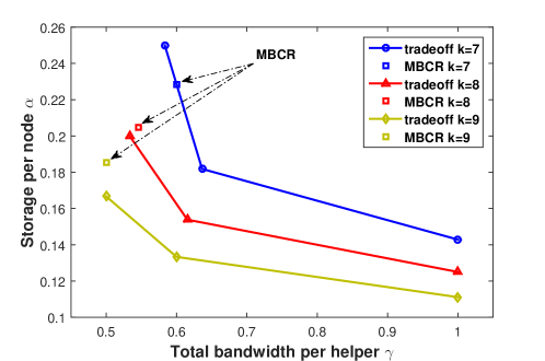
Figure 4: Optimal repair tradeoffs for fixed $e=3$ and different $k\in\{7,8,9\}$. The MBCR point lies on the tradeoff only in the case of $k=7$.

Figure 4 illustrates the functional tradeoff for fixed $e=3,\mathcal{M}=1$ and multiple values of $k\in\{7,8,9\}$ such that $d=k$. As proved in Theorem 12, MBCR codes are optimal centralized repair codes only when $r=1$, which corresponds to $k=7$ in Figure 4. When $e\mid k$, MBCR codes achieve the same bandwidth as MBMR codes, but have a higher storage cost.

Remark 10.

Theorem 12 proves that, when $e\nmid k,r=1$, MBCR codes achieve an interior point on the functional tradeoff that lies near the MBMR point. We note that the existence of this exact-repair interior point does not contradict the infeasibility result in Section V, where we assume $e|k$.

V Infeasibility of the exact- repair interior points

In this section, we study the infeasibility of the interior points on the optimal functional-repair tradeoff for $e\mid k,e\mid d,2e<k$, similarly to [17]. We note that all interior points satisfy $(d-k+e)\beta\leq e\alpha\leq d\beta$. This can be written as $(d^{\prime}-\eta+1)\beta\leq\alpha\leq d^{\prime}\beta$, where $d^{{}^{\prime}}=\frac{d}{e}$ and $\eta=\frac{k}{e}$. This is similar to the single erasure case with reduced parameters. The proof techniques in this section follow along similar lines as [17] and some of the proofs are relegated to the appendix.

Parameterization of the interior points. Let $\alpha=(d^{\prime}-p)\beta-\theta$, namely $e\alpha=(d-ep)\beta-e\theta$ with $p\in\{0,1,\ldots,\eta-1\}$, $\theta\in[0,\beta)$ such that $\theta=0$ if $p=\eta-1$. Points on the functional tradeoff satisfy

$$\mathcal{M}=e\sum\limits_{i=0}^{\eta-1}\min(\alpha,(d^{\prime}-i)\beta).$$

V-A Properties of exact-repair codes

We present a set of properties that exact-repair codes, satisfying the optimal functional tradeoff, must satisfy.

Lemma 13.

For a set $A$ of arbitrary nodes of size $ej$, a set $L$ of nodes of size $e$ such that $L\cap A=\emptyset$, we have

$$I(W_{L},W_{A})=\begin{cases}0,&\qquad j\leq p,\\ e((j-p)\beta-\theta),&\qquad p<j<\eta,\\ e\alpha,&\qquad j\geq\eta.\end{cases}$$ (133)

Proof:

See Appendix -D. ∎

Corollary 2.

For an arbitrary set $L$ of size $e$, and a disjoint set $A$ such that $|A|=em<k$ for some integer $m$, we have

$$H(W_{L}|S_{A}^{L})=H(W_{L}|W_{A})=\min(e\alpha,(d-em)\beta).$$ (134)

Proof:

From Lemma 5, we have $H(W_{L}|S_{A}^{L})\leq\min(e\alpha,(d-em)\beta)$. On the other hand, from Lemma 6,

$$H(W_{L}|S_{A}^{L})\geq H(W_{L}|W_{A})=\min(e\alpha,(d-em)\beta).$$ (135)

Thus, $H(W_{L}|S_{A}^{L})=H(W_{L}|W_{A})=\min(e\alpha,(d-em)\beta).$ ∎

Lemma 14.

In the situation where node $m$ is an arbitrary helper node assisting in the repair of a second set of arbitrary nodes $L$ of size $e$, we have

$$H(S_{m}^{L})=\beta,$$ (136)

irrespective of the identity of the other $d-1$ helper nodes. Moreover, for set $B$ of size $|B|\leq d-k+e$ with $B\cap L=\emptyset$, we have

$$H(S_{B}^{L})=|B|\beta.$$ (137)

Proof:

See Appendix -E. ∎

Helper node pooling. Consider a set $F$ consisting of a collection of $f\leq d+e$ nodes ($f$ is a multiple of $e$), and a subset $R$ of the set $F$ consisting of $er^{\prime}$ nodes, $r^{\prime}\geq 1$. A helper node pooling scenario is a scenario where upon failure of any $e$ nodes $L\subseteq R$, the $d$ helper nodes include all the $f-e$ remaining nodes in $F$. The remaining $d-f+e$ helper nodes are fixed given $L$. Consider a subset of nodes $M\subseteq F\backslash R$. Partition the nodes in $R$ into arbitrary but fixed sets $R_{1},R_{2},\ldots,R_{r^{\prime}},$ each of size $e$. Denote by $S_{M}^{R}=(S^{R_{1}}_{M},\dots S^{R_{r^{\prime}}}_{M})$ the collective transmitted information from helper nodes $M$ to repair $R_{1},\dots,R_{r^{\prime}}$, respectively.

Lemma 15.

In the helper node pooling scenario where $\min(\eta,\frac{f}{e})>p+2\geq r^{\prime}$, for any set of $e$ arbitrary nodes $M\subseteq F\backslash R$, we have

$$H(S_{M}^{R})\leq e(2\beta-\theta).$$ (138)

Proof:

See Appendix -F. ∎

Lemma 16.

In the helper node scenario where $\min\{\eta,\frac{f}{e}\}>p+1\geq r^{\prime}$, for an arbitrary set of $e$ nodes $M\subseteq F\backslash R$, and an arbitrary pair of set of $e$ nodes $L_{1},L_{2}$, it must be that

$$H(S_{M}^{L_{1}}|S_{M}^{L_{2}})\leq e\theta,$$ (139)

and hence

$$H(S_{M}^{R})\leq e(\beta+(r^{\prime}-1)\theta).$$ (140)

Proof:

See Appendix -G. ∎

V-B Non-existence proof

For interior points, $1\leq p\leq\eta-2$. First, we consider the interior points for which $e\alpha$ is a multiple of $\beta$. That is: $e\alpha=(d-ep)\beta,\theta=0$.

Theorem 13.

Exact-repair codes do not exist for the interior points with $\theta=0$.

Proof:

Consider a sub-network $F$ consisting of $d+e$ nodes. The parameters satisfy the condition in Lemma 16. Note that by the regeneration property for any set of $e$ nodes $L\subseteq F$, $H(W_{L}|S_{F-L}^{L})=0$. Moreover, for distinct $M,L_{1},L_{2}\subseteq F$, with $\theta=0$, we have $H(S_{M}^{L_{1}}|S_{M}^{L_{2}})=0$. We partition the nodes in $F$ into groups of size $e$, denoted $L_{i},i=1,2,\dots,d^{\prime}+1$. Then, we write

$$\mathcal{M}\leq H(W_{F})\leq H(S_{F-L_{1}}^{L_{1}},\dots,S_{F-L_{d^{\prime}+1}}^{L_{d^{\prime}+1}}) =H(S^{F-L_{1}}_{L_{1}},\dots,S^{F-L_{d^{\prime}+1}}_{L_{d^{\prime}+1}})$$

$$\leq\sum\limits_{i=1}^{d^{\prime}+1}H(S_{L_{i}}^{F-L_{i}})$$

$$\leq\sum\limits_{i=1}^{d^{\prime}+1}e\beta$$ (141)

$$=(d+e)\beta,$$

where the inequality (141) follows from Lemma 16. On the other hand,

$$\mathcal{M}=\sum_{i=0}^{d^{\prime}-1}\min(e\alpha,(d-ie)\beta)=\sum_{i=0}^{d^{\prime}-1}\min((d-ep)\beta,(d-ie)\beta) =2(d-ep)\beta+\sum_{i=2}^{d^{\prime}-1}\min((d-ep)\beta,(d-ie)\beta)$$

$$\geq 2(d-ep)\beta+(\eta-2)e\beta$$

$$\geq 2e\beta+(d-ep)\beta+(\eta-2)e\beta$$

$$=(d-2e)\beta+(k-2e-ep)\beta$$

$$\geq(d-2e)\beta,$$ (142)

where we assume $1\leq p\leq\eta-2$ (non-MSMR point). Thus, $ep+2e\leq k\leq d$. Both bounds are contradictory, thus proving the impossibility result in the case of $\theta=0$. ∎

Theorem 14.

For any given values of $\mathcal{M}$, exact-repair regenerating codes do not exist for the parameters lying in the interior of the storage-bandwidth tradeoff when $\theta\neq 0$, except possibly for the case $p+2=\eta$ and $\theta\geq\frac{d-ep-e}{d-ep}\beta.$

Proof:

See Appendix -H. ∎

VI Adaptive multi-node repair for MBR codes

In this section, we study multi-node repair for MBR codes, allowing a varying number of helpers and a varying number of failures. In Section IV, we proved that MBMR codes are not achievable for linear exact repair codes, when $2\leq e<k$. When $e=1$, exact MBMR codes are MBR codes and their existence is well established in the literature [43]. Adaptive regenerating codes possess the extra feature that the number of helpers involved in the repair process can be adaptively selected, which provides the storage system with robustness to the network varying conditions [25, 50]. Adaptive MSR codes have been constructed in [35]. On the other hand, adaptive MBR codes have been investigated in [51], in which case optimal repair means that the total repair bandwidth for each number of helpers $d$ is the lowest possible, and is given by $\gamma=\alpha,\forall d_{\text{min}}\leq d\leq d_{\text{max}}$ (assuming the storage per node contains no redundancy). Here $d_{\text{min}},d_{\max}$ are between $k$ and $n-1$. It is shown in [51] that adaptive MBR codes, designed for arbitrary $d$, $d_{\text{min}}\leq d\leq d_{\text{max}}$, are equivalent to MBR codes that are designed for the worst-case number of helpers $d_{\text{min}}$, and they satisfy optimal repair for arbitrary number of helpers $d_{\text{min}}\leq d\leq d_{\text{max}}$. Namely, adaptive MBR codes satisfy for any $d_{\text{min}}\leq d\leq d_{\text{max}}$,

$$d\beta=\alpha,$$ (143)

$$\alpha=\frac{2d_{\min}\mathcal{M}}{-k^{2}+k+2kd_{\min}}=\frac{d_{\min}\mathcal{M}}{d_{\min}k-\binom{k}{2}},$$ (144)

where the storage size $\alpha$ corresponds to the MBR code with $d_{\min}$ helpers.

A natural question of interest is whether there exists an MBR code that efficiently recover from varying number of failures simultaneously. In this section, we investigate the problem of repairing multiple failures in MBR codes under exact repair, for varying number of helpers $d$ and varying number of failures $e$, such that $d_{\text{min}}\leq d\leq d_{\max}$, $1\leq e\leq k$, $e+d\leq n$. First, we derive a lower bound on the multi-node repair bandwidth for MBR codes, which applies to exact and functional codes. We assume that an MBR code is designed for $d$ helpers, and we want to repair $e$ failures. To emphasize the dependency on $e$, denote the total repair bandwidth by $\gamma_{\text{MBR}}(e)$.

Theorem 15.

Consider an $(n,k,d,\alpha,\beta)$ MBR regenerating code, the total repair bandwidth $\gamma_{\text{MBR}}(e)$ needed to repair any set of $1\leq e\leq k$ nodes satisfies

$$\gamma_{\text{MBR}}(e)\geq e\alpha-{e\choose 2}\frac{\alpha}{d}.$$ (145)

Proof:

Assume w.l.o.g that the first $e$ nodes are to be repaired. From [52], at the MBR point, for any set of $A$ nodes of size $m<k$ and for $i\notin A$, we have $H(W_{i}|W_{A})=(d-m)\beta$. Therefore,

$$H(W_{[e]}) =\sum\limits_{i=1}^{e}H(H_{i}|W_{[i-1]})=\sum\limits_{i=1}^{e}(d-i+1)\beta=(ed-{e\choose 2})\beta.$$ (146)

Noting that at the MBR, $\alpha=d\beta$, (145) follows. ∎

We now briefly describe a construction of adaptive MBR codes that simultaneously and efficiently repair single node failures, presented in [51]. Then, we show how to optimally repair multiple failures in this construction.

VI-A Adaptive single-failure MBR construction

The construction is based on product matrix codes [51, 43]. Let $\alpha=\prod\limits_{d=d_{\text{min}}}^{d_{\text{max}}}d$ . Define $z=\frac{\alpha}{d_{\text{min}}}$ and construct the $(\alpha\times\alpha)$ data matrix $M$ as

$$M=\begin{bmatrix}M_{1}&O&\cdots&O\\ O&M_{2}&\cdots&O\\ \vdots&&\ddots&\vdots\\ O&\cdots&O&M_{z}\end{bmatrix},$$ (147)

where $O$ is a $(d_{\text{min}}\times d_{\text{min}})$ zero matrix and each of the submatrices $M_{i}$ is filled with information symbols, and is symmetric and satisfies the structural properties of a product-matrix MBR code for parameters $k$ and $d_{\text{min}}$. For instance, $M_{i}$ is given by

$$M_{i}=\begin{bmatrix}N_{i}&L_{i}\\ L_{i}^{t}&O^{{}^{\prime}}\end{bmatrix},$$ (148)

where $N_{i}$ is a symmetric $(k\times k)$ matrix, $L_{i}$ is $(k\times(d_{\text{min}}-k))$ matrix, and $O^{{}^{\prime}}$ is $(d_{\text{min}}-k)\times(d_{\text{min}}-k)$ zero matrix. let $\Psi$ be an $(zn\times d_{\text{min}})$ Vandermonde matrix, with rows denoted by $\mathbf{\psi}_{j}^{t}$, for $1\leq j\leq zn$. Then, storage node $l$ is associated with

$$\mathbf{w}_{l}^{t}=\begin{bmatrix}\mathbf{\psi}_{(l-1)z+1}^{t},\ldots,\mathbf{\psi}_{lz}^{t}\end{bmatrix}M=\begin{bmatrix}\mathbf{\psi}_{(l-1)z+1}^{t}M_{1},\ldots,\mathbf{\psi}_{lz}^{t}M_{z}\end{bmatrix}.$$

Single node repair. Denote the set of helpers by $\mathcal{H}$ such that $|\mathcal{H}|=d$ and $d_{\text{min}}\leq d\leq d_{\text{max}}$. Let $\Omega$ be an $(z\times z)$ matrix such that $\Omega^{t}$ is a Vandermonde matrix. Assume that node $f$ fails. Let $\Omega_{d}$ an $(\frac{\alpha}{d}\times z)$ containing the first $\frac{\alpha}{d}$ rows of $\Omega$. Moreover, let $\Phi_{i}$ be an $(\alpha\times z)$ matrix

$$\Phi_{i}=\begin{bmatrix}\mathbf{\psi}_{(i-1)z+1}\\ &\ddots&\\ &&\mathbf{\psi}_{iz}\end{bmatrix}.$$

Each helper node $i_{j}\in\mathcal{H}$ transmits $\mathbf{s}_{i_{j},f}^{t}=\mathbf{w}_{i_{j}}^{t}\Phi_{f}\Omega_{d}^{t}$. After simplification, the replacement node obtains

$$\mathbf{w}_{f}^{t}\begin{bmatrix}\Phi_{i_{1}}\Omega_{d}^{t},\ldots,\Phi_{i_{d}}\Omega_{d}^{t}\end{bmatrix}=\mathbf{w}_{f}^{t}\Theta_{\mathcal{H}}$$ (149)

Noting that $\Theta_{\mathcal{H}}$ is invertible [51], the replacement node can thus recover $\mathbf{w}_{f}^{t}$.

VI-B Adaptive multi-node repair in MBR codes

We state our result in the following theorem.

Theorem 16.

Adaptive single-failure MBR regenerating codes with storage per node $\alpha$ and arbitrary number of helpers $d_{\text{min}}\leq d\leq d_{\text{max}}$, presented in[51], can simultaneously and optimally repair $e$ failures with $d$ helpers, for all $d_{\text{min}}\leq d\leq d_{\max}$, $1\leq e\leq k$, $e+d\leq n$.

Proof:

Assume w.l.o.g that the first $e$ nodes failed and $d$ helpers are used, where $d_{\text{min}}\leq d\leq d_{\max}$, $1\leq e\leq k$, $e+d\leq n$. Denote the helpers by the set $\mathcal{H}=\{i_{1},\ldots,i_{d}\}$. First, the repair of node $1$ is done by contacting all the $d$ helpers and downloading $\frac{\alpha}{d}$ symbols from each one of them, using the procedure described for single node repair. Node $2$ is then repaired using only $d_{\text{min}}$ helpers, comprising repaired node $1$ and any other $d_{\text{min}}-1$ helpers in $\mathcal{H}$, such that each helper provides $\frac{\alpha}{d_{\text{min}}}=z$ symbols. The same procedure is then applied repeatedly until recovering the last node $e$ by contacting any $d_{\text{min}}-e+1$ helpers in $\mathcal{H}$ and using contributions from the $e-1$ already repaired nodes. The overall repair bandwidth is given by

$$d\frac{\alpha}{d}+\sum\limits_{i=1}^{e-1}z(d_{\text{min}}-i)=e\alpha-{e\choose 2}\frac{\alpha}{d_{\text{min}}},$$ (150)

which matches the bound in (145), establishing the optimality of the repair procedure. ∎

Remark 11.

Repairing $e$ failures in an $(n,k,d_{\text{min}},\alpha,\beta)$ MBR code separately requires a bandwidth of size $e\alpha$. However, simultaneously repairing $e$ failures using $d\geq d_{\text{min}}$ reduces the bandwidth by ${e\choose 2}\frac{\alpha}{d_{\text{min}}}$ .

Remark 12.

The repair procedure of multiple erasures in Theorem 16 is asymmetric. However, one can always duplicate the code a sufficient number of times to achieve a symmetric repair strategy (e.g. [49]).

VII Conclusion

We studied the problem of centralized repair of multiple erasures in distributed storage systems. We explicitly characterized the optimal functional tradeoff between the repair bandwidth and the storage size per node. For instance, we obtained the expressions of the extreme points on the tradeoff, namely the minimum storage multi-node repair (MSMR) and the minimum bandwidth multi-node repair (MBMR) points. In the case of $e\geq k$, we showed that the tradeoff reduces to a single point, for which we provided a code construction achieving it. We described a general framework for converting single erasure minimum storage regenerating codes to MSMR codes. Then we applied the framework to product-matrix codes and interference alignment codes. Furthermore, we proved that the functional MBMR point is not achievable for linear exact repair codes for $1<e<k$. We also showed that the functional repair tradeoff is not achievable under exact repair, except for maybe a small portion near the MSMR point for $e<k,e\mid k,e\mid d$. Finally, we presented an MBR code that can adaptively and optimally repair varying number of failures with varying number of helpers.

Open problems include the generalization of the non-existence proof of linear exact-repair MBMR regenerating codes to non-linear codes. It is interesting to determine the storage and bandwidth values of an exact minimum bandwidth regenerating code. Moreover, characterization of the storage-bandwidth tradeoff for exact repair for the interior points is still not known.

-A proof of Lemma 4

We first state the following lemma which will be useful in the proof.

Lemma 17.

For fixed $\beta$, the scenario $\mathbf{u}=[e,\ldots,e,r]$ achieves the lowest final value of minimum cut:

$$\lim\limits_{\alpha\to+\infty}f(\mathbf{u})\geq\lim\limits_{\alpha\to+\infty}f([e,\ldots,e,r]),\forall\mathbf{u}\in\mathcal{P},$$ (151)

where $f(\mathbf{u})$ and $\mathcal{P}$ are defined in (4) and (5), respectively.

Proof:

for a specific cut $\mathbf{u}$, we have

$$\lim\limits_{\alpha\to+\infty}f(\mathbf{u}) =\sum\limits_{i=1}^{g}(d-\sum\limits_{j=1}^{i-1}u_{j})\beta$$

$$=d\beta g-\beta\sum\limits_{i=1}^{g}\sum\limits_{j=1}^{i-1}u_{j}=gd\beta-\beta\sum\limits_{i=1}^{g-1}u_{i}(g-i)$$

$$=\beta(dg-g\sum\limits_{i=1}^{g-1}u_{i}+\sum\limits_{i=1}^{g-1}iu_{i})=\beta((d-k)g+\sum\limits_{i=1}^{g}iu_{i}).$$ (152)

To obtain the smallest minimum cut value, we need to solve the following problem

$$\underset{\mathbf{u},g}{\text{minimize}} (d-k)g+\sum\limits_{i=1}^{g}iu_{i}$$ (153)

subject to $$1\leq u_{i}\leq e,$$

$$\sum\limits_{i=1}^{g}u_{i}=k.$$

It can be seen that the solution to (153) is given by $\mathbf{u}=[e,\ldots,e,r]$. ∎

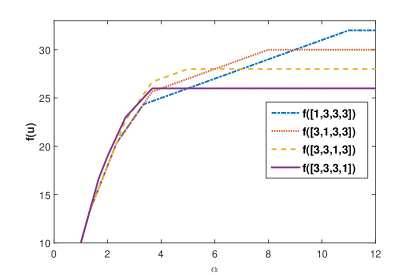
Figure 5: Values of the cut function for different vectors $\mathbf{u}$ for $k=9,d=10,\beta=1$

We now study the different functions $C_{j}(\alpha)$ for $j=0,\ldots,\eta$. An example of the different functions to be analyzed is given in Figure 5, with $k=9,d=10,\beta=1$. It is observed that $\mathbf{u}=[1,3,3,3]$ generates the lowest cut before some threshold $\alpha^{*}=5$, after which the lowest cut is generated by $\mathbf{u}=[3,3,3,1]$. In the following, by analyzing $C_{j}(\alpha)$ for $j=0,\ldots,\eta$, we prove that the above observation holds true in general.

j=0

we have

$$C_{0}(\alpha) =\min(r\alpha,d\beta)+\sum\limits_{i=0}^{\eta-1}\min(e\alpha,(d-r-ie)\beta)=r\min(\alpha,\frac{d\beta}{r})+\sum\limits_{i=0}^{\eta-1}e\min(\alpha,\frac{(d-r-ie)\beta}{e}).$$ (154)

$C_{0}(\alpha)$ is a piecewise linear function with breakpoints given by $\{\frac{d-r-(\eta-1)e}{e}\beta,\frac{d-r-(\eta-2)e}{e}\beta,\ldots,\frac{d-r}{e}\beta,\frac{d}{r}\beta\}$. $C_{0}$ increases from 0 at a slope of $k$. Its slope is then reduced by $e$ by the successive breakpoints and then finally by $r$ until it levels off.

$1\leq j\leq\eta$

for each $j$, we have

$$C_{j}(\alpha) =\sum\limits_{i=0}^{j-1}\min(e\alpha,(d-ie)\beta)+\min(r\alpha,(d-je)\beta)+\sum\limits_{i=j}^{\eta-1}\min(e\alpha,(d-r-ie)\beta)$$

$$=\sum\limits_{i=0}^{j-1}e\min(\alpha,\frac{(d-ie)\beta}{e})+r\min(\alpha,\frac{(d-je)\beta}{r})+\sum\limits_{i=j}^{\eta-1}e\min(\alpha,\frac{(d-r-ie)\beta}{e}).$$ (155)

$C_{j}(\alpha)$ is also piecewise-linear function with non-increasing successive slopes. Its breakpoints are given by

$$\{\frac{d-r-(\eta-1)e}{e}\beta,\ldots,\frac{d-r-je}{e}\beta,\frac{d-(j-1)e}{e}\beta,\ldots,\frac{d}{e}\beta\}\cup\{\frac{d-je}{r}\beta\}.$$

The exact relative position of the breakpoint $\frac{d-je}{r}\beta$ with respect to the other breakpoints of $C_{j}(\alpha)$ depends on the system’s parameters. However, we give a lower bound on $\frac{d-je}{r}\beta$.

$$\frac{d-je}{r}-\frac{d-r-(j-1)e}{e} =\frac{ed-rd-re+r^{2}-j(e^{2}-re)}{re}$$

$$\geq\frac{(e-r)d-re+r^{2}-\eta(e^{2}-re)}{re}$$

$$\geq\frac{(e-r)k-re+r^{2}-\eta(e^{2}-re)}{re}$$

$$=0,$$ (156)

where the first inequality follows by noticing that the expression is decreasing in $j$ and letting $j=\eta$, and the second inequality follows as the corresponding expression is increasing $d$.

Figure 6 illustrates the relative positions of all the breakpoints of $C_{0}(\alpha)$ and $C_{j}(\alpha),j\geq 1$, where for example $\frac{d-je}{r}\in[\frac{d-r-(j-1)e}{e},\frac{d-r-(j-2)e}{e}]$. We denote by $C_{j}(\infty)=\lim\limits_{\alpha\to+\infty}C_{j}(\alpha)$.

Figure 6: relative positions of the breakpoints of $C_{0}(\alpha)$ and $C_{j}(\alpha)$ (with $\beta=1$)

.

Lemma 18.

For $1\leq j\leq\eta$, there exists a point $\alpha_{c}(j)\in[\frac{d}{e},\frac{d}{r}]$ such that

$$C_{0}(\alpha_{c}(j)) =C_{j}(\alpha_{c}(j)),$$ (157)

$$C_{0}(\alpha) \leq C_{j}(\alpha) \text{if }\alpha\leq\alpha_{c}(j),$$

$$C_{0}(\alpha) \geq C_{j}(\alpha) \text{if }\alpha\geq\alpha_{c}(j),$$

$$C_{j}(\alpha) =C_{j}(\infty) \text{if }\alpha\geq\alpha_{c}(j).$$

Proof:

W.l.o.g, assume $\beta=1$. First, we note that

$$C_{0}(\alpha)=C_{j}(\alpha)=k\alpha\text{ for }\alpha\leq\frac{d-r-(j-1)e}{e}.$$

Next, we analyze the behavior of each of the functions $C_{0}(\alpha)$ and $C_{j}(\alpha)$ over the successive intervals $I_{i}\triangleq(\frac{d-r-ie}{e},\frac{d-r-(i-1)e}{e}]$ for $i\in\{j-1,j-2,\ldots,1\}$. Let $x_{i}=\frac{d-r-ie}{e}$ and define $s_{j}(I_{i})$ as the slope of $C_{j}(\alpha)$ just before $\alpha=x_{i}$ . Consider a given interval $I_{i}=(x_{i},x_{i-1}]$, we have

• $C_{0}(\alpha)$ has no breakpoint inside $I_{i}$. Thus, $C_{0}(\alpha)$ increases by

  $$C_{0}(x_{i-1})-C_{0}(x_{i}) =s_{0}(I_{i})-e.$$

• $C_{j}(\alpha)$ has either one or two breakpoints inside $I_{i}$.

  1. in the case of $C_{j}(\alpha)$ has a single breakpoint inside $I_{i}$ (at $\alpha=\frac{d-ie}{e}$), $C_{j}(\alpha)$ increases by

     $$C_{j}(x_{i-1})-C_{j}(x_{i}) =s_{j}(I_{i})\frac{r}{e}+(s_{j}(I_{i})-e)\frac{e-r}{e}=s_{j}(I_{i})-e+r.$$

  2. in the case of $C_{j}(\alpha)$ has two breakpoints inside $I_{i}$, namely at $\alpha=\frac{d-je}{r}$ and $\alpha=\frac{d-ie}{e}$. Let $\Delta=\frac{d-je}{r}-\frac{d-r-ie}{e}$ (c.f. Figure 6). Assuming $\frac{d-je}{r}\leq\frac{d-ie}{e}$, then, $C_{j}(\alpha)$ increases by

     $$C_{j}(x_{i-1})-C_{j}(x_{i})=(s_{j}(I_{i})-r)(1-\Delta-\frac{e-r}{e})+\frac{e-r}{e}(s_{j}(I_{i})-r-e)+s_{j}(I_{i})\Delta=s_{j}(I_{i})-e+\Delta r.$$ (158)

     Assuming $\frac{d-je}{r}\geq\frac{d-ie}{e}$, then, $C_{j}(\alpha)$ increases by

     $$C_{j}(x_{i-1})-C_{j}(x_{i})=\frac{r}{e}s_{j}(I_{i})+(k-e)(\Delta-\frac{r}{e})+(s_{j}(I_{i})-r-e)(1-\Delta)=s_{j}(I_{i})-e+\Delta r,$$ (159)

     which shows that the increase does not depend on the relative position of the two breakpoints.

Now that we have computed the increase increment of each $C_{j}$ over $I_{i}$, we proceed to compare $C_{0}(\alpha)$ and $C_{j}(\alpha)$ for $1\leq j\leq\eta$.

We discuss two cases:

Case 1

Assume $\frac{d-je}{r}\in I_{j_{0}}$ for some $j_{0}\in[1,j-1]$. $j_{0}$ may not exist, which will be discussed in the second case. Based on the above discussion, it can be seen that

$$C_{j}(\alpha)\geq C_{0}(\alpha),\text{ for }\alpha\leq x_{j_{0}}.$$

This can be seen by noticing that $\forall i<j_{0},s_{0}(I_{i})=s_{j}(I_{i})$ and that

$$(C_{j}(x_{i-1})-C_{j}(x_{i}))-(C_{0}(x_{i-1})-C_{0}(x_{i}))=r\geq 0.$$

Over $I_{j_{0}}$, $C_{j}$ also dominates $C_{0}$ at every point as $s_{0}(I_{j_{0}})=s_{j}(I_{j_{0}})$ and

$$(C_{j}(x_{i-1})-C_{j}(x_{i}))-(C_{0}(x_{i-1})-C_{0}(x_{i}))=\Delta r\geq 0.$$

For $i>j_{0}$, we have $s_{0}(I_{i})-s_{j}(I_{i})=r$. Moreover, over each $I_{i},i>j_{0}$, we have

$$(C_{j}(x_{i-1})-C_{j}(x_{i}))-(C_{0}(x_{i-1})-C_{0}(x_{i}))=(s_{j}(I_{i})-e+r)-(s_{0}(I_{i})-e)=0.$$

Combining the last equation and the observation that $C_{j}(x_{j_{0}-1})\geq C_{j}(x_{j_{0}-1})$, it follows that $C_{j}$ continues to dominate $C_{0}$ over the successive intervals $I_{i},i>j_{0}$. So far, we have shown that

$$C_{j}(\alpha)\geq C_{0}(\alpha),\text{ for }\alpha\leq\frac{d-r}{e}.$$

For $\alpha\geq\frac{d-r}{e}$, we observe that $C_{j}$ increases with a slope of $e$ and levels off at $\frac{d}{e}$ while $C_{0}$ increases at smaller slope given by $r$ and levels off at $\frac{d}{r}>\frac{d}{e}$. Moreover, we know from Lemma 17 that $C_{0}$ levels off at a higher value than that of $C_{j}$. Thus, there exists $\alpha_{c}(j)\in[\frac{d}{e},\frac{d}{r}]$ that satisfies (157).

Case 2

Assume $\frac{d-r}{e}<\frac{d-je}{r}\leq\frac{d}{r}$, then, using similar arguments as in the first case, it follows that for $\alpha\leq\frac{d-r}{e}$, $C_{j}(\frac{d-r}{e})\geq C_{0}(\frac{d-r}{e})$. At $\alpha=\frac{d-r}{e}$, $C_{j}(\alpha)$ has a slope of $r+e$, which is higher than that of $C_{0}$, given by $r$. Thus, the slope of $C_{j}$ remains higher than than of $C_{0}$ until $C_{j}$ levels off. Combining these observations with the fact that $C_{0}$ levels off at a higher value, it follows that both curves will intersect only once. Moreover, the intersection at a point at which $C_{j}$ has leveled off i.e., we have $\alpha_{c}(j)\geq\max(\frac{d}{e},\frac{d-je}{r})$. Therefore, (157) holds also in this case. ∎

Using Lemma 18 and the fact that $C_{\eta}$ achieves the smallest final value from Lemma 17, that is $C_{\eta}(\infty)\leq C_{j}(\infty),j\in[0,\eta-1]$, it follows that (14) holds for any $j\in[0,\eta]$. Moreover, as $\alpha_{c}(\eta)\in[\frac{d}{e},\frac{d}{r}]$, $\alpha_{c}(\eta)$ satisfies

$$r\alpha_{c}(\eta)+\sum\limits_{i=0}^{\eta-1}(d-r-ie)\beta=(\eta+1)\beta d-e\beta\frac{\eta^{2}+\eta}{2},$$ (160)

which implies that

$$r\alpha_{c}(\eta)+\eta(d-r-\frac{e\eta}{2}+\frac{e}{2})\beta=(\eta+1)\beta d-e\beta\frac{\eta^{2}+\eta}{2}.$$ (161)

Simplifying the last equation yields (15).

-B Storage-bandwidth tradeoff expression

We start with the case $k=\eta e+r$. The optimization trade-off is

$$\underset{\alpha\geq 0}{\text{minimize}} \alpha$$ (162)

subject to $$C(\alpha)\geq\mathcal{M}.$$

The constraint is a piece-wise linear function $C(\alpha)$ is given by

$$C(\alpha)=\begin{cases}(\eta+1)\beta d-e\beta\eta(\eta+1)/2,&\alpha\geq\alpha_{c},\\ r\alpha+\sum\limits_{j=0}^{\eta-1}b_{j},&\alpha\in[\frac{b_{0}}{e},\alpha_{c}],\\ (r+ie)\alpha+\sum\limits_{j=i}^{\eta-1}b_{j},&\alpha\in[\frac{b_{i}}{e},\frac{b_{i-1}}{e}],\text{ for }i=1,\ldots,\eta-1,\\ k\alpha,&\alpha\leq\frac{b_{\eta-1}}{e},\end{cases}$$ (163)

with $\alpha_{c}=\frac{d+\eta r-\eta e}{r}\beta,b_{i}=(d-r-ie)\beta$ and

$$\sum\limits_{j=i}^{\eta-1}b_{j}=\beta(\eta-i)(d-r-\frac{e(\eta-1+i)}{2})=\gamma\frac{(\eta-i)(-2r+e+2d-\eta e-ei)}{2d}\triangleq\gamma g_{r}(i),$$ (164)

such that

$$g_{r}(i)=\frac{(\eta-i)(-2r+e+2d-\eta e-ei)}{2d}.$$

The expression $C(\alpha)$ increases from 0 to a maximum value given by $\beta((\eta+1)d-\binom{\eta+1}{2})$. To solve (162), we let $\alpha^{*}=C^{-1}(\mathcal{M})$ under the condition $\mathcal{M}\leq\beta((\eta+1)d-\binom{\eta+1}{2})$. Therefore, we obtain,

$$\alpha^{*}=\begin{cases}\frac{\mathcal{M}}{k},\qquad\quad\mathcal{M}\in[0,\frac{kb_{\eta-1}}{e}]\\ \frac{\mathcal{M}-\sum\limits_{j=i}^{\eta-1}b_{j}}{r+ie},\mathcal{M}\in[(r+ie)\frac{b_{i}}{e}+\sum\limits_{j=i}^{\eta-1}b_{j},(r+ie)\frac{b_{i-1}}{e}+\sum\limits_{j=i}^{\eta-1}b_{j}],\text{ for }i=\eta-1,\ldots 1,\\ \frac{\mathcal{M}-\sum\limits_{j=0}^{\eta-1}b_{j}}{r},\mathcal{M}\in[\frac{b_{0}r}{e}+\sum\limits_{j=0}^{\eta-1}b_{j},r\alpha_{c}+\sum\limits_{j=0}^{\eta-1}b_{j}],\end{cases}$$ (165)

with

$$\frac{rb_{i}}{e}+ib_{i}+\sum\limits_{j=i}^{\eta-1}b_{j} =\frac{-\eta^{2}e^{2}+\eta e^{2}-2aer+2dae-e^{2}i^{2}-e^{2}i-2eir-2r^{2}+2dr)}{2de}\gamma$$

$$=\frac{-k^{2}-r^{2}+e(k-r)+2kd-e^{2}(i^{2}+i)-2ier}{2ed}\gamma$$

$$\triangleq\gamma\frac{\mathcal{M}}{f(i)},$$ (166)

such that

$$f_{r}(i)=\frac{2ed\mathcal{M}}{-k^{2}-r^{2}+e(k-r)+2kd-e^{2}(i^{2}+i)-2ier}.$$

Therefore, fixing $\mathcal{M}$ and varying $\gamma$, we write

$$\alpha^{*}=\begin{cases}\frac{\mathcal{M}}{k},&\mathcal{M}\in[0,\frac{kg_{r}(\eta-1)\gamma}{e}],\\ \frac{\mathcal{M}-\gamma g_{r}(i)}{r+ie},&\mathcal{M}\in[\frac{\gamma\mathcal{M}}{f_{r}(i)},\frac{\gamma\mathcal{M}}{f_{r}(i-1)}],\text{ for }i=\eta-1,\ldots 1,\\ \frac{\mathcal{M}-\gamma g_{r}(0)}{r},&\mathcal{M}\in[\frac{\gamma\mathcal{M}}{f_{r}(0)},(g_{r}(0)+\frac{d+ar-ae}{d})\gamma].\end{cases}$$ (167)

As a function of $\gamma$, after simplifications, we obtain the expression of $\alpha^{*}$ as in Theorem 3. We note that there are $\eta$ piece-wise linear portions on the curve. Moreover, the minimum bandwidth point $\gamma_{\text{MBMR}}$ is given by

$$\gamma_{\text{MBMR}}=\frac{\mathcal{M}}{g_{r}(0)+\frac{d+ar-ae}{d}}=\frac{d\mathcal{M}}{d(\eta+1)-e\binom{\eta+1}{2}}.$$ (168)

The expression of $\alpha_{\text{MBMR}}$ is given by

$$\alpha_{\text{MBMR}}=\frac{\mathcal{M}-\gamma_{\text{MBMR}}g(0)}{r} =\gamma_{\text{MBMR}}\frac{d+\eta r-e\eta}{rd}.$$ (169)

in the case of $e\mid k$, we have $r=0$. The expression of the tradeoff is obtained from (167) by setting $r=0$ and eliminating the last line. We note that in this case, there are $\eta-1$ piece-wise linear portions on the trade-off curve.

-C Derivations of (63), (64) and (65) for IA codes

Consider two systematic nodes $l_{1},l_{2}\in[k],l_{1}\neq l_{2}$, starting from (53) and noting that $V^{{}^{\prime}t}U^{{}^{\prime}}=\kappa P^{{}^{\prime}}$, we obtain after simplification

$$r_{l_{1},l_{2}}=\mathbf{v}_{l_{2}}^{{}^{\prime}t}\mathbf{w}_{l_{1}} =\mathbf{v}_{l_{2}}^{{}^{\prime}t}(U^{{}^{\prime}}-\frac{\kappa^{2}}{1+\kappa}V\mathbf{e}_{l_{1}}\mathbf{e}_{l_{1}}^{t}P^{{}^{\prime}})\begin{bmatrix}\bar{s}_{1,{l_{1}}}-\sum\limits_{j\neq l_{1}}p_{j,1}r_{j,l_{1}}\\ \vdots\\ \bar{s}_{k,{l_{1}}}-\sum\limits_{j\neq l_{1}}p_{j,k}r_{j,l_{1}}\\ \end{bmatrix}$$

$$=\kappa\mathbf{e}_{l_{2}}^{t}P^{{}^{\prime}}\begin{bmatrix}\bar{s}_{1,{l_{1}}}-\sum\limits_{j\neq l_{1}}p_{j,1}r_{j,l_{1}}\\ \vdots\\ \bar{s}_{k,{l_{1}}}-\sum\limits_{j\neq l_{1}}p_{j,k}r_{j,l_{1}}\\ \end{bmatrix}$$

$$=\sum\limits_{j\in[k]}(\kappa P^{{}^{\prime}}_{l_{2},j})\bar{s}_{j,l_{1}}-\kappa r_{l_{2},l_{1}}.$$ (170)

Proceeding in a similar way, for a systematic node $l\in[k]$ and a parity node $m\in[k]$, starting from (57), we obtain

$$\bar{s}_{m,l}=\mathbf{v}_{l}^{{}^{\prime}t}\bar{\mathbf{w}}_{m} =\mathbf{v}_{l}^{{}^{\prime}t}((1-\kappa^{2})V+(1+\kappa)U^{{}^{\prime}}\mathbf{e}_{m}\mathbf{e}_{m}^{{}^{t}}P^{t})\begin{bmatrix}s_{1,m}+\frac{\kappa^{2}}{1-\kappa^{2}}\sum\limits_{j\neq m}P_{1,j}^{{}^{\prime}}\bar{r}_{j,m}\\ \vdots\\ s_{k,m}+\frac{\kappa^{2}}{1-\kappa^{2}}\sum\limits_{j\neq m}P_{k,j}^{{}^{\prime}}\bar{r}_{j,m}\end{bmatrix}$$

$$=((1-\kappa^{2})\mathbf{e}_{l}^{t}+(1+\kappa)\kappa P^{{}^{\prime}}_{l,m}\mathbf{e}_{m}^{{}^{t}}P^{t})\begin{bmatrix}s_{1,m}+\frac{\kappa^{2}}{1-\kappa^{2}}\sum\limits_{j\neq m}P_{1,j}^{{}^{\prime}}\bar{r}_{j,m}\\ \vdots\\ s_{k,m}+\frac{\kappa^{2}}{1-\kappa^{2}}\sum\limits_{j\neq m}P_{k,j}^{{}^{\prime}}\bar{r}_{j,m}\end{bmatrix}$$

$$=(1-\kappa^{2}+\kappa(1+\kappa)P_{l,m}^{{}^{\prime}}P_{l,m})s_{l,m}+\sum\limits_{j\in[k]\backslash\{l\}}(\kappa(1+\kappa)P_{l,m}^{{}^{\prime}}P_{j,m})s_{j,m}+\sum\limits_{j\in[k]}(\kappa^{2}P^{{}^{\prime}}_{l,j})\bar{r}_{j,m}.$$ (171)

Finally, consider two parity nodes $m_{1},m_{2}\in[k],m_{1}\neq m_{2}$, starting from (57), we obtain

$$\bar{r}_{m_{1},m_{2}}=\mathbf{u}_{m_{2}}^{t}\bar{\mathbf{w}}_{m_{1}} =\mathbf{u}_{m_{2}}^{t}((1-\kappa^{2})V+(1+\kappa)U^{{}^{\prime}}\mathbf{e}_{m_{1}}\mathbf{e}_{m_{1}}^{{}^{t}}P^{t})\begin{bmatrix}s_{1,m_{1}}+\frac{\kappa^{2}}{1-\kappa^{2}}\sum\limits_{j\neq m_{1}}P_{1,j}^{{}^{\prime}}\bar{r}_{j,m_{1}}\\ \vdots\\ s_{k,m_{1}}+\frac{\kappa^{2}}{1-\kappa^{2}}\sum\limits_{j\neq m_{1}}P_{k,j}^{{}^{\prime}}\bar{r}_{j,m_{1}}\end{bmatrix}$$

$$=\frac{1-\kappa^{2}}{\kappa}\mathbf{e}_{m_{2}}^{t}P^{t}\begin{bmatrix}s_{1,m_{1}}+\frac{\kappa^{2}}{1-\kappa^{2}}\sum\limits_{j\neq m_{1}}P_{1,j}^{{}^{\prime}}\bar{r}_{j,m_{1}}\\ \vdots\\ s_{k,m_{1}}+\frac{\kappa^{2}}{1-\kappa^{2}}\sum\limits_{j\neq m_{1}}P_{k,j}^{{}^{\prime}}\bar{r}_{j,m_{1}}\end{bmatrix}$$

$$=\sum\limits_{j\in[k]}(\frac{1-\kappa^{2}}{\kappa}P_{j,m_{2}})s_{j,m_{1}}+\kappa\bar{r}_{m_{2},m_{1}}.$$ (172)

-D Proof of Lemma 13

Proof:

First, we note that when $j\geq\eta$, $I(W_{L},W_{A})=H(W_{L})-H(W_{L}|A)=H(W_{L})=e\alpha$. In the following, we assume $j<\eta$. We write

$$I(W_{L},W_{A}) =H(W_{L})-H(W_{L}|A)$$

$$=e\alpha-\min(e\alpha,(d-je)\beta)$$ (173)

$$=e(\alpha-\min(\alpha,(d^{\prime}-j)\beta))$$

$$=e(\alpha-(d^{\prime}-j)\beta)^{+}$$

$$=e((j-p)\beta-\theta)^{+},$$

where we use the notation $(x)^{+}\triangleq\max(x,0)$. Here (173) follows from Lemma 6. ∎

-E Proof of Lemma 14

Proof:

Partition the set of $d$ helpers into $A$ and $B$ such that $|A|=k-e$ and $|B|=d-k+e$, such that $m\in B$. We have $H(W_{L}|S_{A}^{L})=\min(e\alpha,(d-k+e)\beta)=(d-k+e)\beta$, as $e\alpha\geq(d-k+e)\beta$ for all points on the tradeoff. Moreover, exact repair requires $H(W_{L}|S_{A}^{L},S_{B}^{L})=0$. Thus, $H(S_{B}^{L})\geq(d-k+e)\beta$. This implies $H(S_{B}^{L})=(d-k+e)\beta$. Moreover, it must hold that $H(S_{m}^{L})=\beta$ in addition to $S_{m}^{L}$ and $S_{m^{\prime}}^{L}$ being independent if $m\neq m^{\prime}$. Moreover, by choosing $M\subseteq B$, one obtains $H(S_{M}^{L})=e\beta$. ∎

-F Proof of Lemma 15

Proof:

If the statement holds true for some $f,r^{\prime}$, then it also holds true for all $f^{\prime}\geq f$ and $r^{\prime\prime}\leq r^{\prime}$. Thus, for the proof, we only need to consider $F=R\cup M,|F|=f=e(p+3),|R|=r^{\prime}e=(p+2)e,|M|=e$.

Consider repair of an arbitrary set of $e$ nodes $L\subseteq R$, where the set of helpers include $M$ and the $e(p+1)$ remaining nodes in $R$. Then, we write

$$I(S_{M}^{L};W_{R}) =I(S_{M}^{L};W_{L},W_{R-{L}})$$

$$=I(S_{M}^{L};W_{R-{L}})+I(S_{M}^{L};W_{L}|W_{R-{L}})$$

$$\geq I(S_{M}^{L};W_{L}|W_{R-{L}})$$

$$=H(W_{L}|W_{R-{L}})-H(W_{L}|W_{R-{L}},S_{M}^{L})$$

$$\geq H(W_{L}|W_{R-{L}})-H(W_{L}|S_{R-{L}}^{L},S_{M}^{L})$$

$$=\min(e\alpha,(d-e(p+1))\beta)-\min(e\alpha,(d-e(p+2))\beta)$$ (174)

$$=(d-e(p+1))\beta-(d-e(p+2))\beta=e\beta.$$

Here (174) follows from Lemma 6 and Corollary 2. Then, we obtain

$$H(S_{M}^{L}|W_{R})=H(S_{M}^{L})-I(S_{M}^{L};W_{R})\leq e\beta-e\beta=0.$$ (175)

Hence, $H(S_{M}^{L}|W_{R})=0.$ Since $L$ is arbitrary, it follows that $H(S_{M}^{R}|W_{R})=0$. It follows from Lemma 13 that

$$H(S_{M}^{R})=I(S_{M}^{R};W_{R})\leq I(W_{M};W_{R})=e(2\beta-\theta).$$

Hence the proof is completed. ∎

-G Proof of Lemma 16

Proof:

The set is $R$ assumed to consist of $|R|=er^{\prime}=e(p+1)$ nodes, and the set $F$ is such that $F=R\cup\{M\}$, $|M|=e$. Similar to Lemma 15,

$$I(S_{M}^{L};W_{R}) \geq H(W_{L}|W_{R-L})-H(W_{L}|S_{R-L}^{L},S_{M}^{L})$$

$$=\min(e\alpha,(d-(r^{\prime}-1)e)\beta)-\min(e\alpha,(d-r^{\prime}e)\beta)$$

$$=(d-pe)\beta-e\theta-(d-(p+1)e)\beta$$

$$=e(\beta-\theta).$$ (176)

Then, it must be that

$$H(S_{M}^{L}|W_{R})=H(S_{M}^{L})-I(S_{M}^{L};W_{R})\leq e\beta-e(\beta-\theta)=e\theta.$$ (177)

Note that the last inequality holds for any set $L\subseteq R$. Next, consider $L_{1},L_{2}\subseteq R$. For this, consider

$$H(S_{M}^{L_{1}},S_{M}^{L_{2}}) =I(W_{R};S_{M}^{L_{1}},S_{M}^{L_{2}})+H(S_{M}^{L_{1}},S_{M}^{L_{2}}|W_{R})$$

$$\leq I(W_{R};W_{M})+H(S_{M}^{L_{1}},S_{M}^{L_{2}}|W_{R})$$

$$=I(W_{R};W_{M})+H(S_{M}^{L_{1}}|W_{R})+H(S_{M}^{L_{2}}|W_{R},S_{M}^{L_{1}})$$

$$\leq e(\beta-\theta)+e\theta+e\theta=e(\beta+\theta),$$ (178)

where the last inequality follows from Lemma 13 and (177). Then, we have

$$H(S_{M}^{L_{1}}|S_{M}^{L_{2}}) =H(S_{M}^{L_{1}},S_{M}^{L_{2}})-H(S_{M}^{L_{2}})$$

$$=H(S_{M}^{L_{1}},S_{M}^{L_{2}})-e\beta$$

$$\leq e(\beta+\theta)-e\beta=e\theta,$$ (179)

where the first equality follows from Lemma 14.

Finally, partitioning the nodes in $R$ into sets $R_{1},R_{2},\ldots,R_{r^{\prime}}$ of size $e$, it follows

$$H(S_{M}^{R})\leq H(S_{M}^{R_{1}})+\sum\limits_{i=2}^{r^{\prime}}H(S_{M}^{R_{i}}|S_{M}^{R_{i-1}})\leq e\beta+e(r^{\prime}-1)\theta.$$ (180)

Thus the proof is completed. ∎

-H Proof of Theorem 14

Proof:

Take a subnetwork $F$ of $d+e$ nodes. Let $L,M\subseteq F$ be two disjoint groups of $e$ nodes. Partition the $d-e$ remaining nodes into two sets, $A$ of cardinality $ep$ and $B$ of cardinality $d-ep-e$. Exact repair requires

$$H(W_{L}|S_{A}^{L},S_{B}^{L},S_{M}^{L}) =0,$$

$$H(W_{M}|S_{A}^{M},S_{B}^{M},S_{L}^{M}) =0.$$ (181)

It follows that

$$H(W_{L},W_{M}|W_{A},S_{B}^{L},S_{B}^{M},S_{M}^{L})=H(W_{L}|W_{A},S_{B}^{L},S_{B}^{M},S_{M}^{L})+H(W_{M}|W_{L},W_{A},S_{B}^{L},S_{B}^{M},S_{M}^{L})=0.$$ (182)

Therefore, we have

$$(S_{B}^{L},S_{B}^{M},S_{M}^{L}) \geq H(W_{L},W_{M}|W_{A})$$

$$=H(W_{L}|W_{A})+H(W_{M}|W_{A},W_{L})$$

$$=H(W_{L})-I(W_{L};W_{A})+H(W_{M})-I(W_{M};W_{A},W_{L})$$

$$=e\alpha-0+e\alpha-e(\beta-\theta)$$ (183)

$$=2e\alpha-e\beta+e\theta$$

$$=2((d-ep)\beta-e\theta)-e\beta+e\theta$$

$$=(2d-2ep-e)\beta-e\theta.$$

Here (183) follows from Lemma 13. We note that the lower bound does not depend on whether $d$ is a multiple of $e$. Next, we obtain an an upper bound on the same quantity.

Partition $B$ into sets of size $e$, denoted by $L_{i}$. We will use $R=L\cup M,r^{\prime}=2,$ in the helper node pooling.

case: $p+2<\eta$

In this case, the parameters satisfy the condition in Lemma 15.

$$H(S_{B}^{L},S_{B}^{M},S_{M}^{L}) \leq\sum\limits_{L_{i}\in B}H(S_{L_{i}}^{L},S_{L_{i}}^{M})+H(S_{M}^{L})$$ (184)

$$\leq\sum\limits_{L_{i}\in B}e(2\beta-\theta)+e\beta$$ (185)

$$=(d-pe-e)(2\beta-\theta)+e\beta$$

$$=(2d-2ep-e)\beta-(d-ep-e)\theta,$$ (186)

where the inequality (185) is obtained using Lemma 14 and Lemma 15. Equations (-H) and (186) are in contradiction if $d-ep-e>e\iff d>e(p+2)$, which is true as $d\geq k=ae>(p+2)e$.

case: $p+2=\eta$

In this case, Lemma 16 is used to derive an upper bound on $H(S_{B}^{L},S_{B}^{M},S_{M}^{L})$. Lemma 16 does not hold if $\eta=2$. It holds for $\eta>2\iff k>2e$. Thus, we consider $k>2e$. We have

$$H(S_{B}^{L},S_{B}^{M},S_{M}^{L}) \leq\sum\limits_{L_{i}\in B}H(S_{L_{i}}^{L},S_{L_{i}}^{M})+H(S_{M}^{L})$$ (187)

$$\leq\sum\limits_{L_{i}\in B}e(\beta+\theta)+e\beta$$ (188)

$$=(d-ep)\beta+(d-ep-e)\theta.$$ (189)

Equations (-H) and (189) are in contradiction when

$$\theta<\frac{d-ep-e}{d-ep}\beta.$$ (190)

∎

References

- [1] M. Zorgui and Z. Wang, “Centralized multi-node repair in distributed storage,” in 2016 54th Annual Allerton Conference on Communication, Control, and Computing (Allerton), Sept 2016, pp. 617–624.
- [2] ——, “Centralized multi-node repair for minimum storage regenerating codes,” in IEEE International Symposium on Information Theory, 2017. [Online]. Available: http://faculty.sites.uci.edu/zhiying/publications/
- [3] S. Ghemawat, H. Gobioff, and S.-T. Leung, “The google file system,” in ACM SIGOPS operating systems review, vol. 37, no. 5. ACM, 2003, pp. 29–43.
- [4] A. G. Dimakis, P. Godfrey, Y. Wu, M. J. Wainwright, and K. Ramchandran, “Network coding for distributed storage systems,” IEEE Trans. Inf. Theory, vol. 56, no. 9, pp. 4539–4551, 2010.
- [5] R. Ahlswede, N. Cai, S.-Y. Li, and R. W. Yeung, “Network information flow,” IEEE Trans. Inf. Theory, vol. 46, no. 4, pp. 1204–1216, 2000.
- [6] T. Ho, M. Médard, R. Koetter, D. R. Karger, M. Effros, J. Shi, and B. Leong, “A random linear network coding approach to multicast,” IEEE Trans. Inf. Theory, vol. 52, no. 10, pp. 4413–4430, 2006.
- [7] N. B. Shah, K. Rashmi, P. V. Kumar, and K. Ramchandran, “Interference alignment in regenerating codes for distributed storage: Necessity and code constructions,” IEEE Trans. Inf. Theory, vol. 58, no. 4, pp. 2134–2158, 2012.
- [8] C. Suh and K. Ramchandran, “Exact-repair MDS code construction using interference alignment,” IEEE Trans. Inf. Theory, vol. 57, no. 3, pp. 1425–1442, 2011.
- [9] Y. Wu and A. G. Dimakis, “Reducing repair traffic for erasure coding-based storage via interference alignment,” in IEEE International Symposium on Information Theory. IEEE, 2009, pp. 2276–2280.
- [10] D. S. Papailiopoulos, A. G. Dimakis, and V. R. Cadambe, “Repair optimal erasure codes through hadamard designs,” IEEE Trans. Inf. Theory, vol. 59, no. 5, pp. 3021–3037, 2013.
- [11] Z. Wang, I. Tamo, and J. Bruck, “Explicit minimum storage regenerating codes,” IEEE Trans. Inf. Theory, vol. 62, no. 8, pp. 4466–4480, Aug 2016.
- [12] A. S. Rawat, O. O. Koyluoglu, and S. Vishwanath, “Progress on high-rate MSR codes: Enabling arbitrary number of helper nodes,” in Information Theory and Applications Workshop (ITA), 2016. IEEE, 2016, pp. 1–6.
- [13] S. Goparaju, A. Fazeli, and A. Vardy, “Minimum storage regenerating codes for all parameters,” IEEE Trans. Inf. Theory, vol. 63, no. 10, pp. 6318–6328, 2017.
- [14] V. R. Cadambe, S. A. Jafar, H. Maleki, K. Ramchandran, and C. Suh, “Asymptotic interference alignment for optimal repair of MDS codes in distributed storage,” IEEE Trans. Inf. Theory, vol. 59, no. 5, pp. 2974–2987, 2013.
- [15] I. Tamo, Z. Wang, and J. Bruck, “Zigzag codes: MDS array codes with optimal rebuilding,” IEEE Trans. Inf. Theory, vol. 59, no. 3, pp. 1597–1616, March 2013.
- [16] M. Ye and A. Barg, “Explicit constructions of optimal-access MDS codes with nearly optimal sub-packetization,” IEEE Trans. Inf. Theory, vol. 63, no. 10, pp. 6307–6317, 2017.
- [17] N. B. Shah, K. V. Rashmi, P. V. Kumar, and K. Ramchandran, “Distributed storage codes with repair-by-transfer and nonachievability of interior points on the storage-bandwidth tradeoff,” IEEE Trans. Inf. Theory, vol. 58, no. 3, pp. 1837–1852, March 2012.
- [18] I. M. Duursma, “Outer bounds for exact repair codes,” arXiv preprint arXiv:1406.4852, 2014.
- [19] ——, “Shortened regenerating codes,” arXiv preprint arXiv:1505.00178, 2015.
- [20] S. Mohajer and R. Tandon, “New bounds on the (n, k, d) storage systems with exact repair,” in IEEE International Symposium on Information Theory (ISIT). IEEE, 2015, pp. 2056–2060.
- [21] B. Sasidharan, K. Senthoor, and P. V. Kumar, “An improved outer bound on the storage-repair-bandwidth tradeoff of exact-repair regenerating codes,” in IEEE International Symposium on Information Theory (ISIT). IEEE, 2014, pp. 2430–2434.
- [22] R. Bhagwan, K. Tati, Y. Cheng, S. Savage, and G. M. Voelker, “Total recall: System support for automated availability management.” in NSDI, vol. 4, 2004, pp. 25–25.
- [23] A. S. Rawat, O. O. Koyluoglu, and S. Vishwanath, “Centralized repair of multiple node failures with applications to communication efficient secret sharing,” arXiv preprint arXiv:1603.04822, 2016.
- [24] P. Hu, C. W. Sung, and T. H. Chan, “Broadcast repair for wireless distributed storage systems,” in 2015 10th International Conference on Information, Communications and Signal Processing (ICICS). IEEE, 2015, pp. 1–5.
- [25] A.-M. Kermarrec, N. Le Scouarnec, and G. Straub, “Repairing multiple failures with coordinated and adaptive regenerating codes,” in International Symposium on Network Coding (NetCod), 2011. IEEE, 2011, pp. 1–6.
- [26] K. W. Shum and Y. Hu, “Cooperative regenerating codes,” IEEE Trans. Inf. Theory, vol. 59, no. 11, pp. 7229–7258, Nov 2013.
- [27] J. Li and B. Li, “Cooperative repair with minimum-storage regenerating codes for distributed storage,” in INFOCOM, 2014 Proceedings IEEE. IEEE, 2014, pp. 316–324.
- [28] M. Ye and A. Barg, “Optimal MDS codes for cooperative repair,” arXiv preprint arXiv:1801.09665, 2018.
- [29] A. Wang and Z. Zhang, “Exact cooperative regenerating codes with minimum-repair-bandwidth for distributed storage,” in INFOCOM, 2013 Proceedings IEEE. IEEE, 2013, pp. 400–404.
- [30] P. Gopalan, C. Huang, H. Simitci, and S. Yekhanin, “On the locality of codeword symbols,” IEEE Trans. Inf. Theory, vol. 58, no. 11, pp. 6925–6934, Nov 2012.
- [31] I. Tamo and A. Barg, “A family of optimal locally recoverable codes,” IEEE Trans. Inf. Theory, vol. 60, no. 8, pp. 4661–4676, Aug 2014.
- [32] N. Prakash, V. Lalitha, and P. V. Kumar, “Codes with locality for two erasures,” in IEEE International Symposium on Information Theory (ISIT), June 2014, pp. 1962–1966.
- [33] W. Song and C. Yuen, “Locally repairable codes with functional repair and multiple erasure tolerance,” arXiv preprint arXiv:1507.02796, 2015.
- [34] Z. Wang, I. Tamo, and J. Bruck, “Optimal rebuilding of multiple erasures in MDS codes,” IEEE Trans. Inf. Theory, vol. 63, no. 2, pp. 1084–1101, 2017.
- [35] M. Ye and A. Barg, “Explicit constructions of high-rate MDS array codes with optimal repair bandwidth,” IEEE Trans. Inf. Theory, vol. 63, no. 4, pp. 2001–2014, 2017.
- [36] R. Li, J. Lin, and P. P. Lee, “Enabling concurrent failure recovery for regenerating-coding-based storage systems: From theory to practice,” IEEE Trans. Comput., vol. 64, no. 7, pp. 1898–1911, 2015.
- [37] V. Guruswami and M. Wootters, “Repairing reed-solomon codes,” IEEE Trans. Inf. Theory, vol. 63, no. 9, pp. 5684–5698, 2017.
- [38] H. Dau, I. Duursma, H. M. Kiah, and O. Milenkovic, “Repairing reed-solomon codes with multiple erasures,” arXiv preprint arXiv:1612.01361, 2016.
- [39] ——, “Repairing reed-solomon codes with two erasures,” in IEEE International Symposium on Information Theory (ISIT). IEEE, 2017, pp. 351–355.
- [40] B. Bartan and M. Wootters, “Repairing multiple failures for scalar MDS codes,” arXiv preprint arXiv:1707.02241, 2017.
- [41] M. Ye and A. Barg, “Repairing Reed-Solomon codes: Universally achieving the cut-set bound for any number of erasures,” arXiv preprint arXiv:1710.07216, 2017.
- [42] J. Chen and K. W. Shum, “Repairing multiple failures in the suh-ramchandran regenerating codes,” in IEEE International Symposium on Information Theory (ISIT), July 2013, pp. 1441–1445.
- [43] K. Rashmi, N. Shah, and P. Kumar, “Optimal exact-regenerating codes for distributed storage at the MSR and MBR points via a product-matrix construction,” IEEE Trans. Inf. Theory, vol. 57, no. 8, pp. 5227–5239, Aug 2011.
- [44] Y. Wu, A. G. Dimakis, and K. Ramchandran, “Deterministic regenerating codes for distributed storage,” in Allerton Conference on Control, Computing, and Communication. Citeseer, 2007, pp. 1–5.
- [45] H. Zhang, H. Li, K. W. Shum, H. Hou, and S. R. Li, “Concurrent regenerating codes,” IET Communications, vol. 11, no. 3, pp. 362–369, 2017.
- [46] D. E. Knuth, The Art of Computer Programming, Volume 1 (3rd Ed.): Fundamental Algorithms. Redwood City, CA, USA: Addison Wesley Longman Publishing Co., Inc., 1997.
- [47] N. Alon and M. Tarsi, “Combinatorial nullstellensatz,” Combinatorics Probability and Computing, vol. 8, no. 1, pp. 7–30, 1999.
- [48] M. Zorgui and Z. Wang, “Centralized multi-node repair regenerating codes,” in IEEE Trans. Inf. Theory (submitted), 2018. [Online]. Available: https://github.com/Marwen-Zorgui/%Centralized_repair_IA.git
- [49] M. Elyasi, S. Mohajer, and R. Tandon, “Linear exact repair rate region of (k+ 1, k, k) distributed storage systems: A new approach,” in IEEE International Symposium on Information Theory (ISIT). IEEE, 2015, pp. 2061–2065.
- [50] V. Aggarwal, C. Tian, V. A. Vaishampayan, and Y.-F. R. Chen, “Distributed data storage systems with opportunistic repair,” in INFOCOM, 2014 Proceedings IEEE. IEEE, 2014, pp. 1833–1841.
- [51] K. Mahdaviani, A. Khisti, and S. Mohajer, “Bandwidth adaptive & error resilient regenerating codes with minimum repair bandwidth,” in IEEE International Symposium on Information Theory (ISIT). IEEE, 2016, pp. 235–239.
- [52] K. Rashmi, N. B. Shah, P. V. Kumar, and K. Ramchandran, “Explicit construction of optimal exact regenerating codes for distributed storage,” in 47th Annual Allerton Conference on Communication, Control, and Computing, 2009. Allerton 2009. IEEE, 2009, pp. 1243–1249.