A New Model of the Chemistry of Ionizing Radiation In Solids: CIRIS

Abstract

The collisions between high-energy ions and solids can result in significant physical and chemical changes to the material. These effects are potentially important for better understanding the chemistry of interstellar and planetary bodies, which are exposed to cosmic radiation and the solar wind, respectively; however, modeling such collisions on a detailed microscopic basis has thus far been largely unsuccessful. To that end, a new model, entitled CIRIS: the Chemistry of Ionizing Radiation in Solids, was created to calculate the physical and chemical effects of the irradiation of solid materials. With the new code, we simulate O₂ ice irradiated with 100 keV protons. Our models are able to reproduce the measured ozone abundances of a previous experimental study, as well as independently predict the approximate thickness of the ice used in that work.

1 Introduction

Irradiation by charged particles is well-known to cause substantial physiochemical changes in condensed matter. Beyond its more obvious connections to medical and material science, a detailed understanding of the effects of irradiation induced processes is of great astrochemical interest, since the galaxy is bathed in cosmic rays. Cosmic rays are a particularly high-energy form of ionizing radiation (MeV - TeV) ¹ comprised mostly of protons, which are thought to be created in supernovae ² or by the super-massive black holes at the centers of galaxies ³. In the interstellar medium, cosmic rays are known to have a strong influence on the chemistry of molecular clouds ⁴. One component of such environments is dust, which, in cold dense regions, is covered by an ice mantle mainly composed of water ⁵, ⁶. Based on the substantial body of experimental studies showing the complexity of irradiation chemistry, such processes represent promising means by which large interstellar molecules could be formed ⁷, particularly in cases where observational results are difficult to reproduce with current astronomical models ⁸ and possible drivers of complex molecule synthesis are not obvious. In the case of interstellar clouds such as TMC-1, which have temperatures of around 10 K and densities of $\sim 10^{4}$ cm^-3, a better understanding of cosmic ray induced irradiation chemistry is particularly required since the interiors of these regions are shielded from most of the interstellar UV radiation field. Though cosmic ray ionization rates are reduced by roughly two orders of magnitudes in these regions ⁹, a steady-state is reached at which ionization rates stabilize. Thus, particularly in dense cold interstellar environments, it is possible that cosmic ray induced chemical processes represent a potentially very efficient pathway to produce complex and even prebiotic molecules.

Although the interstellar chemistry following cosmic ray bombardment of grains has rarely been studied theoretically, Monte Carlo techniques have been used to give a detailed, microscopic view of the chemistry of solids with, however, only a cursory treatment of the role of ion bombardment. The first such stochastic grain chemistry model utilizing a Monte Carlo approach was reported by Chang et al. ¹⁰. This and later models have utilized in particular the continuous-time random-walk Monte Carlo approach of Montroll and Weiss ¹¹, such as the simulation of Chang and Herbst ¹².

Due to its many practical applications, prior interest in modeling irrradiated matter is well known. Most of this previous computational research has focused on simulating particle tracks in the material, which result from the collisions between species in the solid and the irradiating particles. Due to the stochastic nature of these collisions, Monte Carlo methods are a natural choice for such simulations. Well-known models of this type include MOCA ¹³, MARLOWE ¹⁴, TRIM ¹⁵, and that of Pimblott et al. ¹⁶. The subsequent irradiation-induced chemistry that occurs has been followed in a large number of laboratory experiments on ices and bare solids using both high-energy protons and electrons. In spite of this interest, there has been only limited success in combining track calculations with the subsequent chemistry. One of the most detailed of such attempts was the model of Pimblott and LaVerne ¹⁷. In that work, the authors were able to combine realistic track calculations with a simplified chemical network representing the aqueous solution of a Fricke dosimeter; however, in spite of approximations to the chemistry, such as treating the solute as an infinite continuum, they were only able to simulate the radiation induced chemistry for $\sim 1\mu$s, due to the computational expense.

The computational expense of these models reflects the many complex physical and chemical processes associated with the bombardment of solids, which must be considered when using a detailed microscopic approach like molecular dynamics or one of the Monte Carlo methods. The physical processes are initiated when a moving energetic particle collides with some material, which we call the target. In this work, the particles we consider are protons and we refer to these as primary ions; however, if the incoming particle is an electron it is sometimes called the primary electron. These primaries transfer energy to atomic or molecular species in the target through collisions. Some of these collisions ionize species in the material, resulting in the formation of “secondary” electrons, which, in turn, transfer energy collisionally to target species and compound the effects of the primary particle, in large part by causing the formation of additional charged species and secondary electrons ¹⁸. Subsequent charge recombination reactions help drive the formation of radicals and other highly reactive species ¹⁹, which can react via thermal diffusive mechanisms in the solid, albeit much more slowly than the non-thermal irradiation induced processes ¹⁸.

In this paper, we present a code that is designed to simulate these processes over simulated irradiation exposures relevant to experiments and other real-world applications where a better understanding of the resulting effects on the material is desired. This program, with the acronym CIRIS, which stands for the Chemistry of Ionizing Radiation in Solids, represents an initial attempt at the development of a simulation including a unified model of atomic physics and chemistry. Here, we report the use of our code to simulate the chemistry of the experimental system studied by Baragiola et al. ²⁰, hereafter referred to as B99. In that work, solid O₂ ice cooled to 5 K under ultra-high vacuum (UHV) conditions was irradiated with 100 keV protons and ozone was synthesized via proton-induced chemical processes.

This system is particularly well-suited as an initial test of our new code. Due to the novelty of this kind of model, well-constrained experiments such as the one reported by B99 allow for a reasonable comparison with our theoretical data. This comparison is aided by the relative simplicity of the irradiated oxygen ice system. One example of this relative simplicity is the upper limit to the size of observable molecules produced via irradiation; namely, ozone, as found by experimental studies, not only of B99, but also those of Ennis and Kaiser ²¹ and Lacombe et al. ²². In other systems, such as those containing carbon, it may not be obvious to determine the limit of chemical complexity obtainable through these processes and some arbitrary upper limit in molecular size may have to be set in the chemical network.

Molecular oxygen ice is present, not only in the Solar System on icy Jovian moons such like Ganymede ²³, ²⁴ but also in comets. Recently, interest in cometary O₂ ice has increased following the detection of gas-phase O₂ around comet 67P/Churyumov-Gerasimenko ²⁵. It has been speculated by Taquet et al. ²⁶ and Mousis et al. ²⁷ that this molecular oxygen was liberated from the icy body of the comet. If that is indeed true, then this represents a possible immediate application of the current results, since comets experience irradiation from the Solar wind, made up mostly of protons with energies mostly between 1.5 and 10 keV ²⁸, and cosmic rays with energies above $\sim$1 MeV ²⁹ that are not stopped by the Solar wind. Moreover, it is possible that cometary ices are relatively pristine remnants of the parent pre-solar nebula ²⁶. Since observations of interstellar O₂, either in the gas or frozen in ice, have thus far proved mainly unsuccessful ³⁰, ³¹, ³², cometary ice chemistry may provide a crucial window into an as yet poorly understood aspect of interstellar chemistry. Therefore, it is possible that a better understanding of the irradiation chemistry of cometary ices in our Solar system can provide clues as to its possible importance in and contribution to more remote interstellar environments.

The format of the following sections of the paper is as follows. In Section 2 we discuss our model in more detail and give the theory behind the atomic physics and chemistry calculations. In Section 3, we give the results and discuss how these compare with prior experimental work. Finally, in Section 4, we present our summary and conclusions.

2 Model and Theory

In our approach, solids are approximated as a lattice, represented in the program by a three-dimensional array. This structure is comprising two types of sites: strongly bound regular lattice sites on the surface and in the bulk of the solid, and more weakly bound internal interstitial sites ³³. At the start of a simulation, we assume a regular lattice comprised of some material, which in this work is solid O₂. The simulation begins when the first irradiating proton collides with the pristine ice. The primary ion strikes a random surface site at a 90^∘ angle and, as it travels through the solid, the code calculates the relevant physical changes to the material, as described below in Section 2.1. The calculations described there are repeated for every subsequent particle arrival. As given in Section 2.2, in the model times between particle arrivals, neutral species can thermally diffuse through the solid and chemical reactions in Section 2.3 can occur. The model ends when the target material has been exposed to some total amount of irradiation, known as the fluence.

2.1 Monte Carlo modeling of irradiation effects

Collisions between energetic particles, such as protons and electrons, with target species occur randomly along the track of the particle through the solid and are thus well-suited to modeling using Monte Carlo techniques. For so-called “fast” incident ions with energies greater than $\sim$ 1 keV/amu ¹⁸, the timescale for these collisions is very short, relative to the chemical timescale ¹⁸. Because the physical irradiation processes occur much faster than the subsequent chemistry, the model decouples the track calculations from the chemistry while the ion is travelling through the target.

In our code, the arrival rate, in $s^{-1}$, for incoming primary ions is given by

$$k_{\mathrm{ion}}=\phi_{\mathrm{ion}}A_{\mathrm{solid}}$$ (1)

where $\phi_{\mathrm{ion}}$ is the radiation flux in cm^-2 s^-1 and $A_{\mathrm{solid}}$ is the surface area of the solid being irradiated. We assume a Poisson distrubution of waiting times and calculate the next ion arrival using the stochastic relation

$$\tau_{\mathrm{ion}}=-\frac{\mathrm{ln}(R_{\mathrm{n}})}{k_{\mathrm{ion}}}$$ (2)

where $R_{\mathrm{n}}$ is a pseudorandom number between 0 and 1. When an ion hits the ice, thermal diffusion is halted until a special set of calculations, described in section 2.1.1, is completed to determine the changes to the solid caused by the incoming ion.

2.1.1 Track Calculations

Following Bohr ³⁴, we divide collisions between a moving energetic ion and stationary target into two broad categories: those in which energy is transferred to the target nuclei, which are customarily called nuclear, or elastic, collisions, and those in which energy is transferred to the target electrons, which are called electronic, or inelastic, collisions. The inelastic collisions can be further subdivided into ionizations, in which enough energy is imparted to liberate a secondary electron, and electronic excitations of the target atom or molecule. Here, rotational and vibrational excitations are not considered.

Our code calculates the distance to the next collision, $\Delta x$, based on the mean-free-path, $\Lambda_{\mathrm{tot}}$ for an energetic ion with some energy, $E$, given by

$$\Lambda_{\mathrm{tot}}=\frac{1}{n_{\mathrm{target}}\,\sigma_{\mathrm{tot}}}$$ (3)

where $n_{\mathrm{target}}$ is the number density of the target and $\sigma_{\mathrm{tot}}$ is the total cross-section ¹⁶, which is given by

$$\sigma_{\mathrm{tot}}=\sigma_{\mathrm{elastic}}+\sigma_{\mathrm{inelastic}}=\sigma_{\mathrm{elastic}}+\sigma_{\mathrm{ion}}+\sigma_{\mathrm{ex}}$$ (4)

where $\sigma_{\mathrm{ion}}$ and $\sigma_{\mathrm{ex}}$ are the cross-sections for ionization and excitation of the target, respectively ¹⁶. We stochastically determine which of these three types of collisions occurs next based on the relative sizes of the cross-sections using:

$$\text{Collision}\begin{cases}&\text{Ionization for }0<R_{\mathrm{n}}\leq\frac{\sigma_{\mathrm{ion}}}{\sigma_{\mathrm{tot}}}\\ &\text{Excitation for }\frac{\sigma_{\mathrm{ion}}}{\sigma_{\mathrm{tot}}}<R_{\mathrm{n}}\leq\frac{\sigma_{\mathrm{inelastic}}}{\sigma_{\mathrm{tot}}}\\ &\text{Elastic for }\frac{\sigma_{\mathrm{inelastic}}}{\sigma_{\mathrm{tot}}}<R_{\mathrm{n}}\leq 1.\end{cases}$$ (5)

To obtain the distance to the next collision event, we sample from another Poisson distribution using

$$R_{\mathrm{n}}=1-e^{-\Delta x/\Lambda_{\mathrm{tot}}}$$ (6)

where here, a different random number, $R_{\mathrm{n}}$, is used and is equivalent to the probability of the particle travelling a distance of $\Delta x$ to the next collision, given a mean-free-path of $\Lambda_{\mathrm{tot}}$ ¹⁶.

2.1.2 Protons

For protons, we calculate the three key cross-sections for elastic collisions, ionizations and excitations, given in eq. (4) before the first collision, and again after every subsequent one, until the particle leaves the system or its energy falls below an arbitrary cutoff of 100 eV, which is the lower limit to the applicability of our method ³⁵. The average energy loss per unit path length of an ion, labelled A, in a material made of either atoms or molecules, labelled B, is called the stopping, or stopping power ¹⁸, and is given, in the laboratory coordinate system, by

$$\frac{dE}{dx}=n_{\mathrm{B}}(S_{\mathrm{n}}(E)+S_{\mathrm{e}}(E))$$ (7)

where $S_{\mathrm{n}}$ and $S_{\mathrm{e}}$ are the so-called stopping cross-sections for nuclear (elastic) and electronic (inelastic) collisions, respectively, in units of $\mathrm{eV}\;\mathrm{cm}^{2}$, and $n_{\mathrm{B}}$ is the number density of the material. Here, A refers to protons only, and where B is a molecule, we follow Bragg’s rule in approximating the stopping powers as linear combinations of the stopping powers of its constituent atoms ³⁶, ¹⁵.

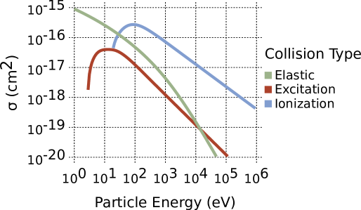
(a) Atomic oxygen

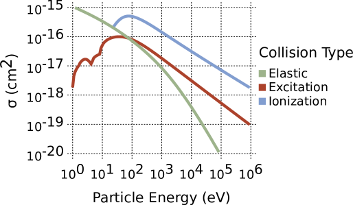
(b) Molecular oxygen

(c) Ozone

Figure 1: Proton-collision cross-sections using parameters listed in Tables 1 and 2.

Our code uses the stopping cross-section, $S_{\mathrm{n}}$, to calculate the collisional cross-section, $\sigma_{\mathrm{elastic}}$. There are many semi-empirical expressions for calculating $S_{\mathrm{n}}$ ¹⁸; we utilize the formalism developed by Ziegler and Biersack ³⁶ and used in the TRIM program ³⁶, ¹⁵ which is valid for ions with energies between $\sim$0.1 keV and several MeV. For an elastic collision between ion A, with energy, $E_{\mathrm{A}}$, and atom B, this is given by

$$S_{\mathrm{n}}(E)=2\pi\frac{\mathcal{A}^{2}}{\gamma E_{\mathrm{A}}}[2\epsilon\,s_{\mathrm{n}}(\epsilon)].$$ (8)

Here, $\gamma$ is the mass fraction, defined as

$$\gamma=\frac{4m_{\mathrm{A}}m_{\mathrm{B}}}{(m_{\mathrm{A}}+m_{\mathrm{B}})^{2}},$$ (9)

and $\mathcal{A}$ is a quantity given by

$$\mathcal{A}=\left(\frac{2m_{\mathrm{A}}}{m_{\mathrm{A}}+m_{\mathrm{B}}}Z_{\mathrm{A}}Z_{\mathrm{B}}e^{2}\right)$$ (10)

where $Z_{\mathrm{A}}$ and $Z_{\mathrm{B}}$ are the nuclear charges of A and B. In equation (8), $\epsilon$ is the Lindhard-Scharff-Schiott (LSS) reduced energy ³⁷, calculated as

$$\epsilon=\frac{32.53\,m_{\mathrm{B}}\,E_{\mathrm{A}}}{Z_{\mathrm{A}}\,Z_{\mathrm{B}}\,(m_{\mathrm{A}}+m_{\mathrm{B}})(Z_{\mathrm{A}}^{0.23}+Z_{\mathrm{B}}^{0.23})}$$ (11)

and $s_{n}(\epsilon)$ is the reduced stopping, which has a value of

$$s_{n}(\epsilon)=\begin{cases}&\frac{\mathrm{ln}(\epsilon)}{2\,\epsilon}\;\;\text{when}\;\;\epsilon>30,\\ \\ &\frac{\mathrm{ln}(1+1.1383\epsilon)}{(\epsilon\;+\;0.01321\epsilon^{0.21226}\;+\;0.19593\epsilon^{0.5})}\;\;\text{otherwise}.\end{cases}$$ (12)

We thus calculate the elastic collisional cross-section from the stopping cross-section using

$$\sigma_{\mathrm{elastic}}=\frac{2S_{\mathrm{n}}(E)}{\gamma E_{\mathrm{A}}}.$$ (13)

These elastic cross-sections typically have values of less than $\sim 10^{-20}$ cm^-2 at energies above approximately 100 keV and approach values of $10^{-16}$ cm^-2 as the incident ion energy decreases.

The kinetic energy transferred from the ion to the target in the elastic collision is found from elementary classical scattering theory ¹⁵ to be

$$E_{\mathrm{kin}}=\frac{4E_{\mathrm{A}}m_{\mathrm{A}}m_{\mathrm{B}}}{m_{\mathrm{A}}+m_{\mathrm{B}}}\mathrm{sin^{2}}\frac{\Theta}{2}$$ (14)

where $\Theta$, the center-of-mass (CM) scattering angle, is obtained using the “Magic Formula” of Biersack and Haggmark ³⁵ and the “universal” potential for ion-target scattering of Ziegler and Biersack ³⁶. It should be noted that the scattering angles are all assumed to be small and thus tracks of the primary ions are approximated with straight line trajectories; however, we calculate these angles explicitly in the code to allow for more accurate modeling of the energy lost in such nuclear-elastic collisions.

Table 1: Proton ionization cross-section parameters

State	$a$	$J$(eV)	$\nu$	$\Omega$	$I$(eV)
Atomic Oxygen
${}^{3}\mathrm{P}_{2}$	20.40	$6.15\times 10^{4}$	0.82	0.75	13.6
Molecular Oxygen
$X\;^{2}\Pi_{g}$	9.56	$4.58\times 10^{4}$	0.61	1.26	12.1
Ozone
$X\;^{1}\mathrm{A}_{1}$	40.00	$1.05\times 10^{5}$	1.00	0.75	12.43

Table 2: Proton excitation cross-section parameters

Excited State	$a$	$J$(eV)	$\nu$	$\Omega$	$W$(eV)
Atomic Oxygen
${}^{1}\mathrm{D}$	0.51	$5.40\times 10^{3}$	1.0	1.0	1.85
${}^{1}\mathrm{S}$	0.075	$8.70\times 10^{3}$	1.0	1.0	4.18
${}^{3}\mathrm{S}$	0.38	$3.72\times 10^{4}$	1.0	1.0	9.53
${}^{5}\mathrm{S}$	0.55	$1.61\times 10^{6}$	1.0	1.0	9.20
Molecular Oxygen
$a^{1}\Delta_{\mathrm{g}}$	0.092	$2.50\times 10^{3}$	0.5	3.0	0.98
$b^{1}\Sigma_{\mathrm{g}}^{+}$	0.11	$4.19\times 10^{3}$	0.5	3.0	1.64
$A^{3}\Sigma_{\mathrm{u}}^{+}$	0.57	$1.76\times 10^{4}$	0.5	0.9	4.5
$B^{3}\Sigma_{\mathrm{u}}^{-}$	4.73	$5.17\times 10^{4}$	0.5	0.75	8.4
9.9 eV peak	0.83	$8.07\times 10^{4}$	0.5	0.85	9.9
Ozone
${}^{1}\mathrm{B}_{2}$	0.84	20.00	0.30	35.00	4.9

For protons, ionization and excitation cross-sections are calculated using the semi-empirical Green-McNeal formula ⁴¹, ⁴²

$$\sigma_{\mathrm{inelastic}}=\sigma_{0}\frac{(Z_{\mathrm{B}}\,a)^{\Omega}(E_{\textrm{A}}-I)^{\nu}}{J^{\Omega+\nu}\;+\;(E_{\textrm{A}}-I)^{\Omega+\nu}}$$ (15)

where $\sigma_{0}=10^{-16}\approx\pi\,r_{0}^{2}$ cm², $Z_{\mathrm{B}}$ is the number of electrons in the target atom or molecule, and $I$ is the ionization threshold. For excitations between bound states, we replace $I$ with $W$, the energy threshold for the particular transition. Listed in Tables 1 and 2 are the species-dependent values of the unitless parameters $\Omega$, $\nu$, and $a$, as well as those of the parameter $J$, which is given in units of energy.

In the O₂ ice system considered here, ionization of neutrals by protons, as well as secondary electrons, leads to the formation of the following cation-secondary electron product pairs:

$$\mathrm{O}\rightarrow\mathrm{O}^{+}+e^{-}$$ (16)

$$\mathrm{O_{2}}\rightarrow\mathrm{O}_{2}^{+}+e^{-}$$ (17)

$$\mathrm{O}_{3}\rightarrow\mathrm{O}_{3}^{+}+e^{-}.$$ (18)

For ionization, the energy deducted from the colliding ion is equal to the sum of the ionization threshold, plus an amount equal to the energy of the resulting secondary electron, which is selected randomly from a skewed Gaussian probability density function¹⁶ with a mean value of 33 eV, the average energy per ion pair for O₂ ⁴³.

Shown in Fig. 1 are the cross-sections as a function of proton energy for collisions with the neutral species we consider in this work, O, O₂, and O₃ using the parameters listed in Tables 1 and 2. For atomic and molecular oxygen, we have used data from Edgar et al. ³⁸. Due to the lack of proton-ozone collisional data, in this work, we have fit measured electron impact ionization ³⁹ and electron impact excitation cross-sections ⁴⁰ to Eq. (15) for use in both proton-ozone and secondary electron-ozone ionization and excitation collisions. As can be seen in Fig. 1, for all of the neutral species considered, the ionization cross-sections of protons for all energies above 100 eV are at least about an order of magnitude larger than either the excitation or elastic collisional cross-sections. Below this energy, elastic collisions are dominant. Fig. 1 also shows the well-known inverse relationship between primary ion energy and total collisional cross-section, i.e. that colliding particles with more energy interact less as they travel through materials than do those with lower energies. This illustrates partially why attempts to measure the galactic cosmic ray energy spectrum are thwarted by the effects of Sun, since the lower energy cosmic rays interact more strongly with the Solar wind ⁴⁴.

2.1.3 Secondary Electrons

Once formed, secondary electrons are placed on a random lattice site next to their parent cations and diffuse away until they are stopped by the solid through energy lost in inelastic collisions. To calculate their trajectories in the material, we utilize a hybrid approach which combines elements of proton travel with our treatment of the hopping of neutral species. As with protons, we calculate a mean-free-path between inelastic collisions; however, in the case of electrons, we use this distance to determine the number of instantaneous jumps from one neighboring lattice site to the next until ionization or excitation occurs. The value used in determining these distances is the sum of the total inelastic collisional cross-section and a constant elastic cross-section equal to the geometrical hard-sphere value of $\sigma^{e}_{\mathrm{elastic}}=10^{-16}$ cm². The actual distance a secondary electron travels between collisions, $\Delta x$, is then calculated as in Eq. (6). Energy loss due to elastic collisions of electrons is not treated rigorously since, for the purposes of chemical changes in the solids, such collisions are of comparatively less importance than excitations and ionizations, due to the mass difference between electrons and bulk species.

The secondary electrons formed by the primary ion are known as “first-generation” secondary electrons and these can, in turn, ionize other species in the bulk, resulting in the formation of later generations of secondary electrons. In this way, a cascade of a few to up to $\sim 10^{4}$ ion-pairs can be formed from a single primary ion ¹⁹. For electron-impact ionization cross sections, we use the semi-empirical formala described in Green and Sawada ⁴⁵ given by:

where, $\sigma_{0}$ is $10^{-16}$ cm² and $A(E)$ is the differential cross-section with respect to energy, calculated using

$$A(E)=\left(\frac{K}{E}+K_{\mathrm{B}}\right)\mathrm{ln}\left(\frac{E}{J}+J_{\mathrm{B}}+\frac{J_{\mathrm{C}}}{E}\right).$$ (20)

The values $\Gamma(E)$ and $T_{0}(E)$ are what Green and Sawada ⁴⁵ refer to as width and resonance factors, respectively, and are given by

$$\Gamma(E)=\Gamma_{\mathrm{S}}\frac{E}{E+\Gamma_{\mathrm{B}}}$$ (21)

$$T_{0}(E)=T_{\mathrm{S}}-\left(\frac{T_{\mathrm{A}}}{E+T_{\mathrm{B}}}\right)\mathrm{eV}.$$ (22)

We assume the more energetic electron, post collision, to be the particle which caused the ionization. Thus, $T_{\mathrm{m}}$, the maximum energy of the new secondary electron, is half the remaining energy of the parent electron after the ionization, i.e. $T_{\textrm{m}}=1/2(E-I)$, where $E$ the energy of the colliding secondary electron and $I$ the ionization threshold. Values used in calculating these cross-sections are given in Table 3.

Table 3: Electron ionization cross-section parameters

State	$K$ (eV)	$K_{\mathrm{B}}$	$J$ (eV)	$J_{\mathrm{B}}$	$J_{\mathrm{C}}$ (eV)	$\Gamma_{\mathrm{S}}$ (eV)	$\Gamma_{\mathrm{B}}$ (eV)	$T_{\mathrm{S}}$ (eV)	$T_{\mathrm{A}}$ (eV)	$T_{\mathrm{B}}$ (eV)
Molecular Oxygen
$X\;^{2}\Pi_{\mathrm{g}}$	0.48	0.00	3.76	0.00	0.00	18.50	12.10	1.86	1000.00	24.20
Atomic Oxygen
${}^{3}\mathrm{P}_{2}$	1.03	0.00	1.81	0.00	0.00	13.00	-0.815	6.41	3450.00	162.00

For electron-impact excitations of bulk species from the ground state to the $j$-th state, we use the formalism developed by Porter ⁴⁶ for allowed transitions, in which the cross-section is given by

$$\sigma_{\mathrm{j}}(E)=\left(\frac{q_{0}\,F_{\mathrm{j}}\left[1-\left(\frac{W}{E}\right)^{\alpha}\right]^{\beta}}{E\,W}\right)\mathrm{ln}\left(\frac{4E\,C}{W}+e\right).$$ (23)

Here $q_{0}=4\pi a^{2}R^{2}$, where is $R$ the Rydberg energy for atomic hydrogen, $F_{\mathrm{j}}$ is the optical oscillator strength, and $\alpha$ and $\beta$ dimensionless values which Porter ⁴⁶ extracted from experiment. $W$ is again the excitation energy threshold and ensures proper shape in the low-energy regime while $C$ ensures proper high-energy falloff. Species-specific values used in this work for calculating these excitation cross-sections can be found in Tables 4 and 5.

Table 4: Electron excitation cross-section parameters for allowed transitions

Excited State	$W$(eV)	$\alpha$	$\beta$	$C$	$F$
Atomic Oxygen
${}^{3}\mathrm{S}$	9.53	0.86	1.44	0.32	0.056
Molecular Oxygen
$B^{3}\Sigma_{\mathrm{u}}^{-}$	8.4	1.19	2.31	0.037	0.25
9.9 eV peak	9.9	1.38	3.44	0.62	0.029

Table 5: Electron excitation cross-section parameters for forbidden transitions

Excited State	$W$(eV)	$\alpha$	$\beta$	$\Omega$	$F$
Atomic Oxygen
${}^{1}\mathrm{D}$	1.96	1.00	2.00	1.00	0.010
${}^{1}\mathrm{S}$	4.18	0.50	1.00	1.00	0.0042
${}^{5}\mathrm{S}$	10.60	19.20	10.50	2.69	0.013
Molecular Oxygen
$a^{1}\Delta_{\mathrm{g}}$	0.98	3.00	1.00	3.00	0.0005
$b^{1}\Sigma_{\mathrm{g}}^{+}$	1.64	3.00	1.00	3.00	0.0005
$A^{3}\Sigma_{\mathrm{u}}^{+}$	4.50	1.00	1.00	0.90	0.021

Our calculated values for the electron cross-sections, using the parameters given in Tables 3, 4, and 5, are shown in Fig. 2. Comparison with Fig. 1 shows that the cross-sections for electron impact are generally smaller than the equivalent values for protons at the same energy.

(a) Atomic oxygen

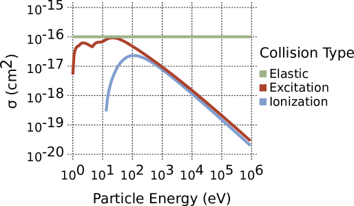
(b) Molecular oxygen

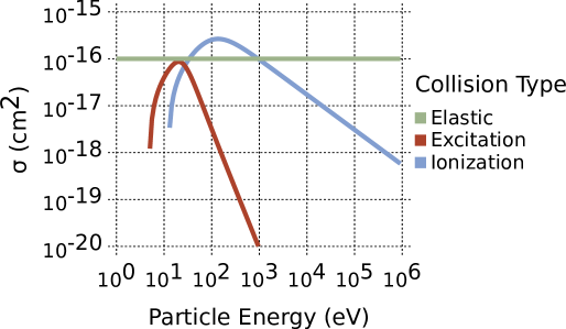
(c) Ozone

Figure 2: Electron-collision cross-sections calculated using parameters from Tables 3, 4, and 5.

Energy is deducted from secondary electrons until a lower threshold of 4 eV is reached, at which point a secondary electron enters the sub-excitation regime. Sub-excitation secondary electrons are thought to be the delivery mechanism for $\sim$10-20% of the energy deposited in the solid by the primary ion ⁴⁸, and affect the chemistry through a variety of mechanisms, such as the resonant process of dissociative electron attachment (DEA) ⁴⁹. We choose 4 eV as our lower energy threshold since it corresponds approximately to the low energy limit of the resonance which leads to DEA in O₂ ⁴⁹.

As listed in Table 6, we assume that sub-excitation electrons are destroyed in one of two ways. One possibility is through charge recombination with a neighboring cation. The other is by reaction with a randomly chosen neighboring neutral species via DEA to form an anion. These anions then react with nearby cations formed in previous ionization collisions at the end of the track calculation phase, at which time all remaining charged species are neutralized by such fast ion-ion reactions ¹⁸.

Table 6: Secondary electron reactions

ID#	Electron Attachment	$f_{\mathrm{branching}}$	Source
1	$\mathrm{O}+e^{-}\rightarrow\mathrm{O}^{-}$	1.00	50
2	$\mathrm{O}_{2}+e^{-}\rightarrow\mathrm{O}^{-}+\mathrm{O}$	1.00	49
3	$\mathrm{O}_{3}+e^{-}\rightarrow\mathrm{O}^{-}+\mathrm{O_{2}}$	1.00	51
ID#	Electron Recombination	$f_{\mathrm{branching}}$	Source
4	$\mathrm{O}^{+}+e^{-}\rightarrow\mathrm{O(^{1}\mathrm{D})}$	1.00	52
5	$\mathrm{O}_{2}^{+}+e^{-}\rightarrow 2\mathrm{O}$	0.20	53
6	$\mathrm{O}_{2}^{+}+e^{-}\rightarrow 2\mathrm{O(^{1}\mathrm{D})}$	0.36	53
7	$\mathrm{O}_{2}^{+}+e^{-}\rightarrow\mathrm{O}+\mathrm{O(^{1}\mathrm{D})}$	0.44	53
8	$\mathrm{O}_{3}^{+}+e^{-}\rightarrow\mathrm{O_{2}}+\mathrm{O}$	0.06	54
9	$\mathrm{O}_{3}^{+}+e^{-}\rightarrow 3\mathrm{O}$	0.26	54
10	$\mathrm{O}_{3}^{+}+e^{-}\rightarrow 3\mathrm{O(^{1}\mathrm{D})}$	0.0094	54
11	$\mathrm{O}_{3}^{+}+e^{-}\rightarrow\mathrm{O}+2\mathrm{O(^{1}\mathrm{D})}$	0.20	54
12	$\mathrm{O}_{3}^{+}+e^{-}\rightarrow 2\mathrm{O}+\mathrm{O(^{1}\mathrm{D})}$	0.47	54

2.2 Continuous-time random walk chemical modeling

In the chemical phase of the model, ground-state neutral species in the bulk can diffuse throughout the crystal lattice of the solid and reactions can occur. The Monte Carlo technique used for modeling the chemistry of the solid is the continuous-time random walk method initially developed by Montroll and Weiss ¹¹, which was further developed by Chang et al. ¹⁰ and others ¹², ⁵⁵, ⁵⁶, ⁵⁷ for studying molecular formation on interstellar dust grains. In this scheme, the interstitial sites facilitate bulk diffusion by allowing species to hop from one interstitial site to another with a low barrier. Normal lattice species are, effectively, immobile and do not become interstitial species; however, if a species on a normal lattice site dissociates or reacts, the products can become interstitial. Moreover, an interstitial species can hop to a lattice defect site to become a normal lattice species. A cartoon representation of these possible moves is given in Fig. 1 of Chang and Herbst ¹².

Hopping rates are parameterized by three species-specific values: the binding energy for surface species, $E_{\mathrm{D}}$; the barrier against diffusion for surface species, $E_{\mathrm{b1}}$; and, the barrier against diffusion for bulk species, $E_{\mathrm{b2}}$. We approximate the surface barrier against diffusion as being $E_{\mathrm{b1}}=0.5E_{\mathrm{D}}$ following the approximation used in Garrod and Herbst ⁵⁸. The bulk barrier against diffusion is assumed to be $E_{\mathrm{b2}}=0.7E_{\mathrm{D}}$ ¹².

For any surface species, the rate coefficient for hopping, $b_{1}$, given by

$$b_{1}=\nu\;\mathrm{exp}\left(-\frac{E_{\mathrm{b1}}}{T}\right)$$ (24)

where $T$ is the temperature of the solid and $\nu$ is the trial frequency, which has a value of $1.0\times 10^{12}$ s^-112, ⁵. Similarly, the rate coefficient for bulk species is

$$b_{2}=\nu\;\mathrm{exp}\left(-\frac{E_{\mathrm{b2}}}{T}\right).$$ (25)

Moreover, on the surface, our Monte Carlo technique allows for the possibility of desorption into the gas phase with a rate coefficient of

$$b_{3}=\nu\;\mathrm{exp}\left(-\frac{E_{\mathrm{D}}}{T}\right).$$ (26)

Whether a surface species hops or desorbs is based on a competitive mechanism based on a random number, $R_{\mathrm{D}}$, to determine the outcome:

$$\text{Outcome}\begin{cases}&\text{Desorption for }0<R_{\mathrm{D}}\leq\frac{b_{3}}{b_{3}+b_{1}}\\ &\text{Diffusion for }\frac{b_{3}}{b_{3}+b_{1}}<R_{\mathrm{D}}\leq 1\end{cases}$$ (27)

Because the primary focus of this work is on modeling the chemistry of the irradiated O₂ system, and because the model is not coupled to any gas-phase chemical system, we have disabled the desorption of surface species. Even when enabled, however, such thermal desorption is negligible, given the low ice temperature of 5 K and the high reactivity of the most weakly bound species, atomic oxygen.

Reactions in the model are assumed to proceed via the diffusive (Langmuir-Hinshelwood) mechanism, and can occur when species hop to sites occupied by possible co-reactants, and products can be formed. If the reaction has a barrier, a competitive mechanism is also utilized to determine whether the reaction proceeds or the hopping species diffuses away. If one of the co-reactants occupies a normal bulk lattice site and there are multiple products, the one with the higher binding energy will be placed at the site, with the rest being randomly placed in the surrounding interstitial sites. On the surface, only the normal lattice sites can be occupied, i.e. it is assumed that there are no available interstitial sites on the surface.

The waiting time between hops, $\tau$, for a species on the surface is given by

$$\tau_{\mathrm{surf}}=-\frac{\mathrm{ln}(R_{\mathrm{D}})}{b_{1}+b_{3}},$$ (28)

while for bulk species, the time is

$$\tau_{\mathrm{bulk}}=-\frac{\mathrm{ln}(R_{\mathrm{D}})}{b_{2}}.$$ (29)

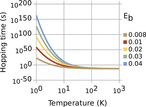
Figure 3: Hopping times for neutral species as a function of system temperature and diffusion barrier height.

As shown in Fig. 3, bulk hopping times are affected by both the system temperature and the height of the diffusion barrier. Above about 100 K, further increases in temperature have little or no effect on the hopping time; however, there is a strong temperature dependence below 10 K and this effect becomes larger with increasing diffusion barriers. As described in detail in Chang and Herbst ¹², the waiting time until the next action is stored in a data structure that also contains the type and current coordinates of each species in the system. After a hop, the model searches the waiting list and the species associated with the shortest waiting moves next.

2.3 Chemical Network

In their work, B99 fit their experimental data with a simplified chemical network consisting of:

$$\mathrm{O_{2}}\rightarrow 2\mathrm{O}$$ (30)

$$\mathrm{O_{3}}\rightarrow\mathrm{O}+\mathrm{O_{2}}$$ (31)

$$\mathrm{O}+2\mathrm{O}_{2}\rightarrow\mathrm{O}_{3}+\mathrm{O_{2}}$$ (32)

$$\mathrm{O}+\mathrm{O}_{3}\rightarrow\mathrm{O}_{2}+\mathrm{O}_{2}$$ (33)

where here, reactions (30) and (31) are irradiation induced dissociations, and reactions (32) and (33) are assumed to proceed via thermal diffusion in the solid. Our network expands on the work of B99, in part, by including electronically excited neutral species, as shown in Table 7. We are able to do this since our method of calculating the tracks of the proton and secondary electrons allows us to determine the final state of a species after undergoing an excitation collision; however, our ability to do so is limited by the scarcity of data on the reactivity and product pathways of species in most of these excited states. For instance, though we explicitly consider excitation of O₂ from its triplet ground state to both excited singlet and triplet states, as shown by the cross-sectional parameters in Tables 2-5, the available theoretical and experimental kinetic data is almost entirely for the ${}^{1}\Delta$ state. Given this discrepancy between the available cross-sectional and kinetic data, in our network, we denote all electronically excited O₂ as O₂(${}^{1}\Delta$). We similarly denote the other excited neutral species in our network using the term symbol of the best studied higher state.

Table 7: Chemical network. The activation energies and branching fractions are taken from gas-phase studies.

ID#	Neutral-Neutral Reactions	$f_{\mathrm{branching}}$	$E_{\mathrm{A}}$(kJ/mol)	Source
13	$\mathrm{O}+\mathrm{O}\rightarrow\mathrm{O_{2}(^{1}\Delta)}$	1.00	0.00	59
14	$\mathrm{O}+\mathrm{O_{2}}\rightarrow\mathrm{O_{3}(^{1}\mathrm{B}_{2})}$	1.00	0.00	60
15	$\mathrm{O}+\mathrm{O_{3}}\rightarrow 2\mathrm{O}_{2}$	1.00	17.12	61
16	$\mathrm{O_{3}}+\mathrm{O_{3}}\rightarrow 3\mathrm{O_{2}}$	1.00	77.41	62
17	$\mathrm{O(^{1}D)}+\mathrm{O}\rightarrow 2\mathrm{O}$	0.50	0.00	63
18	$\mathrm{O(^{1}D)}+\mathrm{O}\rightarrow\mathrm{O_{2}(^{1}\Delta)}$	0.50	0.00	See text
19	$\mathrm{O(^{1}D)}+\mathrm{O_{2}}\rightarrow\mathrm{O}+\mathrm{O_{2}}$	0.50	0.00	60
20	$\mathrm{O(^{1}D)}+\mathrm{O_{2}}\rightarrow\mathrm{O_{3}(^{1}\mathrm{B}_{2})}$	0.50	0.00	See text
21	$\mathrm{O(^{1}D)}+\mathrm{O_{3}}\rightarrow 2\mathrm{O}_{2}$	1.00	0.00	64
22	$\mathrm{O_{2}(^{1}\Delta)}+\mathrm{O}\rightarrow\mathrm{O}+\mathrm{O_{2}}$	0.50	0.00	65
23	$\mathrm{O_{2}(^{1}\Delta)}+\mathrm{O}\rightarrow\mathrm{O_{3}(^{1}\mathrm{B}_{2})}$	0.50	0.00	See text
24	$\mathrm{O_{2}(^{1}\Delta)}+\mathrm{O_{2}}\rightarrow 2\mathrm{O_{2}}$	1.00	0.00	66
25	$\mathrm{O_{2}(^{1}\Delta)}+\mathrm{O_{3}}\rightarrow 2\mathrm{O_{2}}+\mathrm{O}$	1.00	23.61	60
26	$\mathrm{O(^{1}D)}+\mathrm{O(^{1}D)}\rightarrow 2\mathrm{O}$	0.50	0.00	See text
27	$\mathrm{O(^{1}D)}+\mathrm{O(^{1}D)}\rightarrow\mathrm{O_{2}(^{1}\Delta)}$	0.50	0.00	See text
28	$\mathrm{O(^{1}D)}+\mathrm{O_{2}(^{1}\Delta)}\rightarrow\mathrm{O}+\mathrm{O_{2}}$	0.50	0.00	65
29	$\mathrm{O(^{1}D)}+\mathrm{O_{2}(^{1}\Delta)}\rightarrow\mathrm{O_{3}(^{1}\mathrm{B}_{2})}$	0.50	0.00	See text
30	$\mathrm{O(^{1}D)}+\mathrm{O_{3}(^{1}\mathrm{B}_{2})}\rightarrow 2\mathrm{O}_{2}$	1.00	0.00	See text
31	$\mathrm{O_{2}(^{1}\Delta)}+\mathrm{O_{2}(^{1}\Delta)}\rightarrow 2\mathrm{O_{2}}$	1.00	3.23	67
32	$\mathrm{O_{2}(^{1}\Delta)}+\mathrm{O_{3}(^{1}\mathrm{B}_{2})}\rightarrow 2\mathrm{O_{2}}+\mathrm{O}$	1.00	23.61	See text
33	$\mathrm{O_{3}(^{1}\mathrm{B}_{2})}+\mathrm{O_{3}(^{1}\mathrm{B}_{2})}\rightarrow 3\mathrm{O_{2}}$	1.00	77.41	See text
34	$\mathrm{O_{3}(^{1}\mathrm{B}_{2})}+\mathrm{O}\rightarrow 2\mathrm{O}_{2}$	1.00	$17.12$	See text
35	$\mathrm{O_{3}(^{1}\mathrm{B}_{2})}+\mathrm{O_{2}}\rightarrow 2\mathrm{O}_{2}+\mathrm{O}$	1.00	$23.61$	See text
36	$\mathrm{O_{3}(^{1}\mathrm{B}_{2})}+\mathrm{O_{3}}\rightarrow 3\mathrm{O_{2}}$	1.00	77.41	See text
ID#	Ion Recombinations	$f_{\mathrm{branching}}$	$E_{\mathrm{A}}$(kJ/mol)	Source
37	$\mathrm{O}_{2}^{+}+\mathrm{O}_{2}^{-}\rightarrow\mathrm{O_{2}}(^{1}\Delta)+\mathrm{O_{2}}$	1.00	0.00	68
38	$\mathrm{O}_{2}^{+}+\mathrm{O}^{-}\rightarrow\mathrm{O_{2}}(^{1}\Delta)+\mathrm{O}$	1.00	0.00	69
39	$\mathrm{O}_{2}^{-}+\mathrm{O}^{+}\rightarrow\mathrm{O_{2}}(^{1}\Delta)+\mathrm{O}$	1.00	0.00	69
40	$\mathrm{O}^{+}+\mathrm{O}^{-}\rightarrow 2\mathrm{O(^{1}D)}$	1.00	0.00	See text
41	$\mathrm{O^{+}}+\mathrm{O_{3}^{-}}\rightarrow\mathrm{O(^{1}D)}+\mathrm{O_{3}(^{1}\mathrm{B}_{2})}$	1.00	0.00	See text
42	$\mathrm{O^{+}}+\mathrm{O_{3}^{-}}\rightarrow 2\mathrm{O_{2}(^{1}\Delta)}$	1.00	0.00	See text
43	$\mathrm{O^{-}}+\mathrm{O_{3}^{+}}\rightarrow\mathrm{O(^{1}D)}+\mathrm{O_{3}(^{1}\mathrm{B}_{2})}$	1.00	0.00	See text
44	$\mathrm{O^{-}}+\mathrm{O_{3}^{+}}\rightarrow 2\mathrm{O_{2}(^{1}\Delta)}$	1.00	0.00	See text
45	$\mathrm{O_{2}^{-}}+\mathrm{O_{3}^{+}}\rightarrow\mathrm{O_{3}(^{1}\mathrm{B}_{2})}+\mathrm{O_{2}}(1\Delta)$	1.00	0.00	See text
46	$\mathrm{O_{2}^{+}}+\mathrm{O_{3}^{-}}\rightarrow\mathrm{O_{3}(^{1}\mathrm{B}_{2})}+\mathrm{O_{2}}(1\Delta)$	1.00	0.00	See text
47	$\mathrm{O_{3}^{+}}+\mathrm{O_{3}^{-}}\rightarrow 3\mathrm{O_{2}(^{1}\Delta)}$	1.00	0.00	See text

In our code, we assume that neutrals in excited electronic states either react immediately with a neighboring species or relax back to the ground state if there are no possible nearest neighbor co-reactants. The important role excited species play in the chemistry of the irradiated oxygen ice system is illustrated by the following two reactions:

$$\mathrm{O}(^{3}\mathrm{P})+\mathrm{O_{3}}\rightarrow 2\mathrm{O_{2}}$$

$$\mathrm{O}(^{1}\mathrm{D})+\mathrm{O_{3}}\rightarrow 2\mathrm{O_{2}}.$$

Here, the reaction between ozone and the triplet ground state of atomic oxygen has been measured to have a barrier of about 0.2 eV ⁶¹, whereas no barrier has been reported for the reaction between excited singlet atomic oxygen and ozone ⁶⁰.

Following B99, we have drawn heavily on previous research in atmospheric chemistry in compiling our network ⁶⁴, ⁶⁰, ⁶¹; however, in some cases we have been unable to find data on certain reactions, particularly for those involving two electronically excited species. For these, we have based the product channels and branching fractions on similar reactions. Since the chemistry here is occurring in an ice, we have added additional pathways to some of the gas-phase reactions to account for solid-phase effects. For instance, to the previously studied ⁶³ gas-phase reaction

$$\mathrm{O}+\mathrm{O}(^{1}\mathrm{D})\rightarrow 2\mathrm{O}$$

we have added the additional product channel

$$\mathrm{O}+\mathrm{O}(^{1}\mathrm{D})\rightarrow\mathrm{O_{2}}$$

to account for the trapping and stabilization of products in the ice.

Ion-ion recombinations present unique challenges in our model, since there are a number of product channels involving species that can be formed in a number of different excited states. For simplicity, where we have been unable to find data on these processes, we base the product channels on the corresponding neutral-neutral reactions, but with products assumed to be electronically excited, as with:

$$\mathrm{O^{-}}+\mathrm{O_{3}^{+}}\rightarrow 2\mathrm{O_{2}(^{1}\Delta)}$$

$$\mathrm{O^{+}}+\mathrm{O_{3}^{-}}\rightarrow 2\mathrm{O_{2}(^{1}\Delta)},$$

which were based on the reaction between singlet atomic oxygen and ozone.

One class of reactions not present in our network consists of those between ions and neutral species. These are often barrierless and are known to be of significant astrochemical importance ⁷⁰. We do not include these since we assume in this work that ions are quickly neutralized via charge recombination reactions, as suggested by previous theoretical and experimental studies ²⁰, ¹⁸. This is done due to the uncertain diffusion barriers of charged species in solids, and the significant influence of effects which we do not consider in this work, such as Coulombic forces.

3 Results and Discussion

As an initial test of our approach, we simulated the experiment described in B99 in which O₂ is partially converted to O₃. Listed in Table 8 are the physical conditions we take from that work. We assume an initial pure O₂ ice at a constant temperature of 5 K, connected to a helium cryostat. The ice studied in B99 had a thickness of $\sim 10\;\mu m$. In this work we model a $\sim 0.1\;\mu$m thick ice, due both to computational expense and because our interest is ultimately in the chemistry of the ice mantles of interstellar dust grains, which are thought to reach a maximum thickness on the order of $\sim 0.01\;\mu$m ⁷¹. In our code, the simulation begins when the first proton collides with the pristine ice. Following B99, we assume an initial proton energy of 100 keV and a flux of $10^{11}\;\mathrm{cm}^{-2}\;\mathrm{s}^{-1}$ . The model continues to follow subsequent proton arrivals and hopping of species in the ice until an upper fluence limit of $10^{17}$ protons/cm² is reached, where fluence is defined as the total irradiation exposure per unit surface area. It is used in comparing the results of irradiation in a way that is less dependent on the specific flux of particles to which the material is exposed.

Table 8: Model parameters

Physical Conditions from B99	Value
Temperature	5 K
Ice Density [O2]	$1.313\times 10^{22}\;\mathrm{cm}^{-3}$
Initial Proton Energy	100 keV
Proton Flux	$1.0\times 10^{11}\;\mathrm{cm}^{-2}\;\mathrm{s}^{-1}$
Species	Binding Energy to O2 (eV)
O	$2.15\times 10^{-2}$
O2	$7.85\times 10^{-2}$
O3	$6.41\times 10^{-2}$

Using the parameters listed in Table 8, our code predicts that each proton undergoes a collision in the bulk of the ice approximately every 300 Å, or about three times, given the thickness of the simulated ices in this work. On average, protons in these simulations lose on the order of $\sim 10^{2}$ eV, or 0.1$\%$ of their initial energy, by the time they exit the system. We can, however, arbitrarily fix the distance between proton collisions to be some smaller value. By thus increasing the number of collisions, and thus the energy deposited in the system by each proton, we can approximate the effects of having a thicker ice. From the formula for the stopping power, given in Eq. (7), one can derive the energy lost by a proton travelling in a straight path through any given solid to be

$$\Delta E=\Delta x\sum_{n}\frac{Q_{n}}{\Lambda_{n}},$$ (34)

where $\Delta x$ is some path length and the sum is over $n$ inelastic processes, with each resulting in an average energy loss, $Q_{n}$, by the primary ion and having a mean-free-path of $\Lambda_{n}$. If $\Delta x$ is the total thickness of the solid, $\Delta E$ approximates the total energy lost by the primary ion, which is proportional to ice thickness and inversely proportional to the mean-free-path between energy loss events.

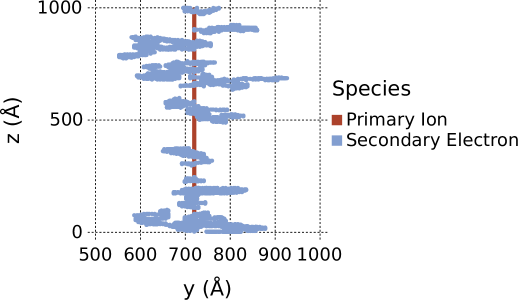
(a) $y$-$z$ track structure

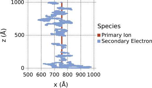
(b) $x$-$z$ track structure

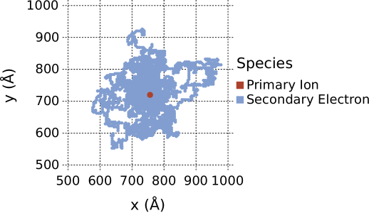
(c) $x$-$y$ track structure

Figure 4: Sample track structure in which a proton collides with a pristine O₂ ice with fixed collision distance of $\Delta x=33$ Å.

Shown in Figs. 4(a)-4(c) is an example of a track calculation in which, starting with pristine O₂ ice, we fixed the distance between collisions to be 33 Å, corresponding to a total cross-section larger than the real value by about an order of magnitude. Here the proton enters the ice at $z=0$ Å, with an entry angle of 90^∘ relative to the surface, and travels in a nearly straight path through the material until it exits at $z=1000$ Å. In Figs. 4(a)-4(c) the path of the proton is represented by a red line and secondary electron paths are given in blue. CIRIS performs such a track calculation for every proton arrival. Given the simulated size of our ice, to reach a fluence of $10^{17}$ protons/cm², our code calculates more than $10^{6}$ such proton arrivals.

Between track calculations, neutral species diffuse through the solid and can react with their neighbors. The rate of this diffusive chemistry is governed, in part, by the hopping rates of each of the reactants. In our code, we calculate these hopping rates using Eqs. (24) - (26). These values are functions of both the temperature of the solid and the barrier against diffusion, which we approximate as 50% and 70% of the desorption energy, $E_{\mathrm{D}}$, of the relevant adsorbate-substrate pair for surface and bulk diffusion, respectively. For O₂-O₂, we have a measured value of $E_{\mathrm{D}}^{\mathrm{O_{2}}}=7.85\times 10^{-2}$ eV from an experimental study by Acharyya et al. ⁷². Lacking other data, one could make the crude assumption that atomic oxygen desorption is $\sim$ 0.5 times this value, and ozone desorption as 1.5 times this value, giving $E_{\mathrm{D}}^{\mathrm{O}}=3.92\times 10^{-2}$ eV and $E_{\mathrm{D}}^{\mathrm{O_{3}}}=1.18\times 10^{-1}$ eV for O and O₃, respectively. Unfortunately, we were unable to find much other previous work on O-O₂ or O₃-O₂ desorption energies; however, Cuppen and Herbst ⁷³ estimate these values to be $E_{\mathrm{D}}^{\mathrm{O}}=4.74\times 10^{-3}$ eV and $E_{\mathrm{D}}^{\mathrm{O_{3}}}=1.03\times 10^{-2}$ eV for O and O₃ adsorbed on an O₂ substrate. Here, we assume that the values derived from the work of Acharyya et al. ⁷² represent a rough upper limit, while those in Cuppen and Herbst ⁷³ represent a lower limit, and use the average of the two. This gives values of $E_{\mathrm{D}}^{\mathrm{O}}=2.15\times 10^{-2}$ eV for O and $E_{\mathrm{D}}^{\mathrm{O_{3}}}=6.41\times 10^{-2}$ eV for O₃. B99 assumed that the concentration of atomic oxygen in their ice remained very low throughout the experiment, given its reactivity with molecular oxygen. We find that, in our models at 5 K, values for the O-O₂ diffusion barriers above $E_{\mathrm{B}}^{\mathrm{O}}\sim 2.60\times 10^{-2}$ eV lead to a large buildup of atomic oxygen in the ice which is most likely unphysical. Values lower than this, such as the one used here, result effectively in a constant near-zero concentration of atomic oxygen in the ice, as it reacts quickly with surrounding species.

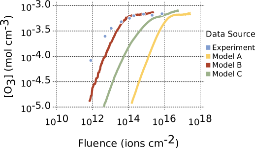
Figure 5: Ozone abundances both as calculated by CIRIS and from B99.

Plotted in Fig. 5 are ozone abundances as a function of proton fluence for the experimental data of B99, as well as several calculated abundance curves. Shown in yellow are data from Model A, in which the distances between proton collisions are calculated on-the-fly based on the magnitude of the energy-dependent cross-sections, as given by Eq. (3). A comparison between the experimental data and this model shows that, in both, ozone abundances increase at roughly the same rate before reaching $\sim 7\times 10^{-4}$ mol cm^-3. After abundances have reached this quasi steady-state value, further irradiation results in only marginal increases in ozone. The fluence at which such an inflection in growth occurs, however, is much larger in the model than measured in B99. This discrepancy is likely due to the differing ice thicknesses considered. Since the ices used in the experimental study were roughly two orders of magnitude thicker than the $\sim 0.1\;\mu$m ice considered in this work, each proton which hit the surface deposited less energy in our base model simulation. To illustrate this effect, we include simulations in Fig. 5,Models B and C, in which the distance between proton collisions was artificially reduced from our calculated value of $\sim 300$ Å, to 3.3 and 33 Å, respectively. These data show that, as more energy per proton is transferred to the solid, the theoretical results approach the experimental values. From Fig. 5, one can also see that the best agreement between our model and the experiment is obtained when $\Delta x=3.3$ Å. Given the thickness of our simulated ice, this means that the proton collides $\sim 300$ times before exiting the system. If one used the Model A results for protons of $\sim 300$ Å  between collisions, our model would predict an ice thickness of $\sim 10^{5}$ Å, or 10 $\mu$m, approximately equal to the actual thickness of the ice studied in B99.

The chemistry behind the ozone abundances given in Fig. 5 begins with the arrival of the first proton. The secondary electrons which form along the track of this primary ion are the main drivers of atomic oxygen production through both dissociative attachment with O₂ and dissociative recombination with O${}_{2}^{+}$. Atomic oxygen is mainly depleted through reaction with O₂, resulting in the formation of the ozone which begins to build up in the ice. This reaction between triplet O and triplet O₂ continues to be the primary formation route for ozone throughout the simulation. Once formed, ozone is destroyed through two main non-thermal pathways which occur as a result of continued irradiation. The first of these is through direct ionization by both the primary ion and secondary electrons, resulting in O${}_{3}^{+}$, which is destroyed via the charge neutralizations with either secondary electrons or anions, which occur at the end of each track calculation phase of the code. The other main destruction mechanism for ozone is reaction with singlet atomic and molecular oxygen, both of which are formed either through direct excitation or as a product of ion-ion and ion-electron recombinations.

4 Summary and Conclusions

In this work, we have presented a new stochastic model which calculates the physical and chemical changes of solids exposed to high-energy protons. Beginning with pure O₂ ice we are able to follow, on a collision-by-collision basis, the tracks of energetic protons and secondary electrons. The reactive species, such as atomic oxygen, which form as a result of the non-thermal processes induced by the irradiation cause significant chemical changes in the ice, even at the very low temperatures considered in this work where thermal diffusive chemistry is inefficient. As shown in Fig. 5, we are able to reproduce both the quasi-steady-state abundances of ozone in such an irradiated material, as well as predict the approximate thickness of the ice studied by B99.

Though our ultimate goal is to better understand the degree to which interactions between cosmic rays and interstellar grain ice mantles contribute to the formation of complex molecules, the techniques presented here are not specific to the chemistry of these extreme environments, and can be applied to other systems as well. One area of practical interest where CIRIS can compliment experimental work is in modeling irradiated polymers, such as poly(vinyl chloride) or PVC. These materials are widely used in environments in which they are exposed to ionizing radiation ⁷⁴. Previous experimental work has investigated PVC radiolysis ⁷⁵, and our code could compliment such studies by providing a means to investigate possible radiolysis pathways, or to simulate the system under physical conditions and exposures not practical or obtainable in the laboratory. Ionizing radiation also poses serious health and safety risks for any future missions to Mars and the Moon, and our code could be used to evaluate potential radiation shielding materials, such as those composed of polymers. This type of shielding is generally more effective at stopping energetic ions than metals, but poses a greater risk of structural failure due to prolonged exposure or flammability, in part, from radiolysis products like gaseous H₂ ⁷⁶, ⁷⁵. By allowing for simulations of the physiochemical evolution of potential shielding materials, use of CIRIS could aid mission planners in selecting the safest, most effective solutions.

A major consideration for future applications to other systems is the availability, or lack thereof, of relevant experimental data. In calculating tracks and collisional probabilities for each neutral species considered in this work, our code draws on cross-sectional data for electron and proton impact ionization and excitation. For the chemistry, we rely on desorption energies to calculate hopping rates, and kinetic studies to determine the branching fractions. Unfortunately, there is often significant uncertainty in desorption energies, as is the case for O-O₂ binding. For the kinetics of charge recombination processes such as ion-ion and ion-electron reactions, the unique properties of storage rings allow for experiments, such as the one reported by Zhaunerchyk et al. ⁵⁴, that can furnish exactly the kind of data which can be directly used in our code, i.e. dissociation pathways, the electronic states of products, and branching fractions. Though we have had to rely mostly on previous gas-phase studies in modeling the comparatively simple O₂ ice system, this approach is not equally applicable for all systems. For instance, Ribeiro et al. ⁷⁷ irradiated CH₃CN ice and observed products with notably different abundances from what would be expected in the gas phase, likely because of the influence of the condensed medium on the non-thermal ion and electron induced chemistry. Such experimental work is of significant value when considering irradiation chemistry on a microscopic level and future applications should focus on systems where solid state

Nevertheless, this model may represent a first-step towards a better understanding of complex, interconnected phenomena. Future versions of our code will focus on improvements that will enable us to examine other aspects of the irradiation of a solid in more detail, despite the promising results reported here of our simulations of the O₂ ice system. First, we would like to consider displacement of lattice species due to elastic collisions in more detail. Improving these aspects will allow us to better model the changes to the ice lattice caused by collisions between bulk species and the primary ion, as well as to begin examining additional processes associated with ion-solid collisions, such as sputtering, in which bound species on or near the surface of the target material are released into the gas phase. Another aspect of the model that is important to continue developing is electron transport. This aspect is treated in more detail by the CASINO ⁷⁸ and PENELOPE ⁷⁹ models, and it may be possible to incorporate the theory they employ into future versions of CIRIS. Related to this, electrostatic effects such as Coulombic forces could be incorporated that could allow for a better picture of the motion of charged species in the solid. Improvements such as these will enable us to better investigate irradiation induced non-thermal desorption mechanisms. In addition to sputtering, these improvements include desorption induced by electronic transitions (DIET), Auger stimulated ion desorption (ASID), and electron stimulated ion desorption (ESID) ⁷⁷. These processes are of particular astrochemical interest, because they represent a means by which the complex molecules formed on interstellar dust grain surfaces can be

C.N.S. wishes to thank the Advanced Research Computing Services (ARCS) center at the University of Virginia for use of the RIVANNA supercomputer. E.H. wishes to thank the National Science Foundation for continuing to support the astrochemistry program at the University of Virginia. This research has made use of NASA’s Astrophysics Data System Bibliographic Services.

References

- Ikhsanov 1991 N. R. Ikhsanov, Astrophysics and Space Science, 1991, 184, 297–311.
- Baade and Zwicky 1934 W. Baade and F. Zwicky, Proceedings of the National Academy of Science, 1934, 20, 259–263.
- Abraham et al. 2007 J. Abraham, P. Abreu, M. Aglietta, C. Aguirre, D. Allard, I. Allekotte, J. Allen, P. Allison, C. Alvarez, J. Alvarez-Muñiz, M. Ambrosio, L. Anchordoqui, S. Andringa, A. Anzalone, C. Aramo, S. Argirò, K. Arisaka, E. Armengaud, F. Arneodo, F. Arqueros, T. Asch, H. Asorey, P. Assis, B. S. Atulugama, J. Aublin, M. Ave, G. Avila, T. Bäcker, D. Badagnani, A. F. Barbosa, D. Barnhill, S. L. C. Barroso, P. Bauleo, J. Beatty, T. Beau, B. R. Becker, K. H. Becker, J. A. Bellido, S. BenZvi, C. Berat, T. Bergmann, P. Bernardini, X. Bertou, P. L. Biermann, P. Billoir, O. Blanch-Bigas, F. Blanco, P. Blasi, C. Bleve, H. Blümer, M. Bohác̆ová, C. Bonifazi, R. Bonino, M. Boratav, J. Brack, P. Brogueira, W. C. Brown, P. Buchholz, A. Bueno, N. G. Busca, K. S. Caballero-Mora, B. Cai, D. V. Camin, R. Caruso, W. Carvalho, A. Castellina, O. Catalano, G. Cataldi, L. Cazón-Boado, R. Cester, J. Chauvin, A. Chiavassa, J. A. Chinellato, A. Chou, J. Chye, P. D. J. Clark, R. W. Clay, E. Colombo, R. Conceição, B. Connolly, F. Contreras, J. Coppens, A. Cordier, U. Cotti, S. Coutu, C. E. Covault, A. Creusot, J. Cronin, S. Dagoret-Campagne, K. Daumiller, B. R. Dawson, R. M. de Almeida, C. De Donato, S. J. de Jong, G. De La Vega, W. J. M. de Mello Junior, J. R. T. de Mello Neto, I. De Mitri, V. de Souza, L. del Peral, O. Deligny, A. D. Selva, C. D. Fratte, H. Dembinski, C. Di Giulio, J. C. Diaz, C. Dobrigkeit, J. C. D’Olivo, D. Dornic, A. Dorofeev, J. C. d. Anjos, M. T. Dova, D. D’Urso, M. A. DuVernois, R. Engel, L. Epele, M. Erdmann, C. O. Escobar, A. Etchegoyen, P. F. S. Luis, H. Falcke, G. Farrar, A. C. Fauth, N. Fazzini, A. Fernández, F. Ferrer, S. Ferry, B. Fick, A. Filevich, A. Filipc̆ic̆, I. Fleck, R. Fonte, C. E. Fracchiolla, W. Fulgione, B. García, D. García Gámez, D. Garcia-Pinto, X. Garrido, H. Geenen, G. Gelmini, H. Gemmeke, P. L. Ghia, M. Giller, H. Glass, M. S. Gold, G. Golup, F. G. Albarracin, M. G. Berisso, R. G. Herrero, P. Gonçalves, M. G. do Amaral, D. Gonzalez, J. G. Gonzalez, M. González, D. Góra, A. Gorgi, P. Gouffon, V. Grassi, A. Grillo, C. Grunfeld, Y. Guardincerri, F. Guarino, G. P. Guedes, J. Gutiérrez, J. D. Hague, J. C. Hamilton, P. Hansen, D. Harari, S. Harmsma, J. L. Harton, A. Haungs, T. Hauschildt, M. D. Healy, T. Hebbeker, D. Heck, C. Hojvat, V. C. Holmes, P. Homola, J. Hörandel, A. Horneffer, M. Horvat, M. Hrabovský, T. Huege, M. Iarlori, A. Insolia, F. Ionita, A. Italiano, M. Kaducak, K. H. Kampert, B. Keilhauer, E. Kemp, R. M. Kieckhafer, H. O. Klages, M. Kleifges, J. Kleinfeller, R. Knapik, J. Knapp, D. H. Koang, A. Kopmann, A. Krieger, O. Krömer, D. Kümpel, N. Kunka, A. Kusenko, G. La Rosa, C. Lachaud, B. L. Lago, D. Lebrun, P. LeBrun, J. Lee, M. A. L. de Oliveira, A. Letessier-Selvon, M. Leuthold, I. Lhenry-Yvon, R. López, A. Lopez Agüera, J. L. Bahilo, M. C. Maccarone, C. Macolino, S. Maldera, M. Malek, G. Mancarella, M. E. Manceñido, D. Mandat, P. Mantsch, A. G. Mariazzi, I. C. Maris, D. Martello, J. Martínez, O. M. Bravo, H. J. Mathes, J. Matthews, J. A. J. Matthews, G. Matthiae, D. Maurizio, P. O. Mazur, T. McCauley, M. McEwen, R. R. McNeil, M. C. Medina, G. Medina-Tanco, A. Meli, D. Melo, E. Menichetti, A. Menschikov, C. Meurer, R. Meyhandan, M. I. Micheletti, G. Miele, W. Miller, S. Mollerach, M. Monasor, D. M. Ragaigne, F. Montanet, B. Morales, C. Morello, E. Moreno, J. C. Moreno, C. Morris, M. Mostafá, M. A. Muller, R. Mussa, G. Navarra, J. L. Navarro, S. Navas, L. Nellen, C. Newman-Holmes, D. Newton, T. N. Thi, N. Nierstenhöfer, D. Nitz, D. Nosek, L. Noz̆ka, J. Oehlschläger, T. Ohnuki, A. Olinto, V. M. Olmos-Gilbaja, M. Ortiz, S. Ostapchenko, L. Otero, D. P. Selmi-Dei, M. Palatka, J. Pallotta, G. Parente, E. Parizot, S. Parlati, S. Pastor, M. Patel, T. Paul, V. Pavlidou, K. Payet, M. Pech, J. Pȩkala, R. Pelayo, I. M. Pepe, L. Perrone, S. Petrera, P. Petrinca, Y. Petrov, D. Ngoc, D. Ngoc, T. N. P. Thi, A. Pichel, R. Piegaia, T. Pierog, M. Pimenta, T. Pinto, V. Pirronello, O. Pisanti, M. Platino, J. Pochon, T. A. Porter, P. Privitera, M. Prouza, E. J. Quel, J. Rautenberg, S. Reucroft, B. Revenu, F. A. S. Rezende, J. R̆ídký, S. Riggi, M. Risse, C. Rivière, V. Rizi, M. Roberts, C. Robledo, G. Rodriguez, D. R. Frías, J. R. Martino, J. R. Rojo, I. Rodriguez-Cabo, G. Ros, J. Rosado, M. Roth, B. Rouillé-d’Orfeuil, E. Roulet, A. C. Rovero, F. Salamida, H. Salazar, G. Salina, F. Sánchez, M. Santander, C. E. Santo, E. M. Santos, F. Sarazin, S. Sarkar, R. Sato, V. Scherini, H. Schieler, F. Schmidt, T. Schmidt, O. Scholten, P. Schovánek, F. Schüssler, S. J. Sciutto, M. Scuderi, A. Segreto, D. Semikoz, M. Settimo, R. C. Shellard, I. Sidelnik, B. B. Siffert, G. Sigl, N. S. De Grande, A. Smialkowski, R. s̆mída, A. G. K. Smith, B. E. Smith, G. R. Snow, P. Sokolsky, P. Sommers, J. Sorokin, H. Spinka, R. Squartini, E. Strazzeri, A. Stutz, F. Suarez, T. Suomijärvi, A. D. Supanitsky, M. S. Sutherland, J. Swain, Z. Szadkowski, J. Takahashi, A. Tamashiro, A. Tamburro, O. Taşcău, R. Tcaciuc, D. Thomas, R. Ticona, J. Tiffenberg, C. Timmermans, W. Tkaczyk, C. J. T. Peixoto, B. Tomé, A. Tonachini, D. Torresi, P. Travnicek, A. Tripathi, G. Tristram, D. Tscherniakhovski, M. Tueros, V. Tunnicliffe, R. Ulrich, M. Unger, M. Urban, J. F. V. Galicia, I. Valiño, L. Valore, A. M. van den Berg, V. van Elewyck, R. A. Vázquez, D. Veberic̆, A. Veiga, A. Velarde, T. Venters, V. Verzi, M. Videla, L. Villaseñor, S. Vorobiov, L. Voyvodic, H. Wahlberg, O. Wainberg, T. Waldenmaier, P. Walker, D. Warner, A. A. Watson, S. Westerhoff, G. Wieczorek, L. Wiencke, B. Wilczyńska, H. Wilczyński, C. Wileman, M. G. Winnick, H. Wu, B. Wundheiler, J. Xu, T. Yamamoto, P. Younk, E. Zas, D. Zavrtanik, M. Zavrtanik, A. Zech, A. Zepeda and M. Ziolkowski, Science, 2007, 318, 938–943.
- Grenier et al. 2015 I. A. Grenier, J. H. Black and A. W. Strong, Annual Review of Astronomy and Astrophysics, 2015, 53, 199–246.
- Hasegawa and Herbst 1993 T. I. Hasegawa and E. Herbst, Monthly Notices of the Royal Astronomical Society, 1993, 261, 83–102.
- Herbst and van Dishoeck 2009 E. Herbst and E. F. van Dishoeck, Annual Review of Astronomy and Astrophysics, 2009, 47, 427–480.
- Abplanalp et al. 2016 M. J. Abplanalp, S. Gozem, A. I. Krylov, C. N. Shingledecker, E. Herbst and R. I. Kaiser, Proceedings of the National Academy of Sciences, 2016, 113, 7727–7732.
- Corby et al. 2015 J. F. Corby, P. A. Jones, M. R. Cunningham, K. M. Menten, A. Belloche, F. R. Schwab, A. J. Walsh, E. Balnozan, L. Bronfman, N. Lo and A. J. Remijan, Monthly Notices of the Royal Astronomical Society, 2015, 452, 3969–3993.
- Rimmer et al. 2012 P. B. Rimmer, E. Herbst, O. Morata and E. Roueff, Astronomy & Astrophysics, 2012, 537, A7.
- Chang et al. 2005 Q. Chang, H. M. Cuppen and E. Herbst, Astronomy and Astrophysics, 2005, 434, 599–611.
- Montroll and Weiss 1965 E. W. Montroll and G. H. Weiss, Journal of Mathematical Physics, 1965, 6, 167.
- Chang and Herbst 2014 Q. Chang and E. Herbst, The Astrophysical Journal, 2014, 787, 135.
- Paretzke 1974 H. G. Paretzke, Fourth symposium on microdosimetry, Commision of European Communities, Luxembourg, 1974.
- Robinson and Torrens 1974 M. T. Robinson and I. M. Torrens, Physical Review B, 1974, 9, 5008.
- Ziegler and Manoyan 1988 J. F. Ziegler and J. M. Manoyan, Nuclear Instruments and Methods in Physics Research B, 1988, 35, 215–228.
- Pimblott et al. 1996 S. M. Pimblott, J. A. LaVerne and A. Mozumder, The Journal of Physical Chemistry, 1996, 100, 8595–8606.
- Pimblott and LaVerne 2002 S. M. Pimblott and J. A. LaVerne, The Journal of Physical Chemistry A, 2002, 106, 9420–9427.
- Johnson 1990 R. E. Johnson, Energetic Charged-Particle Interactions with Atmospheres and Surfaces, Springer, 1990, p. 84.
- Mason et al. 2014 N. J. Mason, B. Nair, S. Jheeta and E. Szymańska, Faraday Discussions, 2014, 168, 235.
- Baragiola et al. 1999 R. A. Baragiola, C. L. Atteberry, D. A. Bahr and M. M. Jakas, Nuclear Instruments and Methods in Physics Research Section B: Beam Interactions with Materials and Atoms, 1999, 157, 233–238.
- Ennis and Kaiser 2012 C. Ennis and R. I. Kaiser, The Astrophysical Journal, 2012, 745, 103.
- Lacombe et al. 1997 S. Lacombe, F. Cemic, K. Jacobi, M. N. Hedhili, Y. Le Coat, R. Azria and M. Tronc, Physical review letters, 1997, 79, 1146.
- Spencer et al. 1995 J. R. Spencer, W. M. Calvin and M. J. Person, Journal of Geophysical Research: Planets, 1995, 100, 19049–19056.
- Calvin and Spencer 1997 W. M. Calvin and J. R. Spencer, Icarus, 1997, 130, 505–516.
- Bieler et al. 2015 A. Bieler, K. Altwegg, H. Balsiger, A. Bar-Nun, J.-J. Berthelier, P. Bochsler, C. Briois, U. Calmonte, M. Combi, J. De Keyser, E. F. van Dishoeck, B. Fiethe, S. A. Fuselier, S. Gasc, T. I. Gombosi, K. C. Hansen, M. Hässig, A. Jäckel, E. Kopp, A. Korth, L. Le Roy, U. Mall, R. Maggiolo, B. Marty, O. Mousis, T. Owen, H. Rème, M. Rubin, T. Sémon, C.-Y. Tzou, J. H. Waite, C. Walsh and P. Wurz, Nature, 2015, 526, 678–681.
- Taquet et al. 2016 V. Taquet, K. Furuya, C. Walsh and E. F. van Dishoeck, Monthly Notices of the Royal Astronomical Society, 2016, 462, S99–S115.
- Mousis et al. 2016 O. Mousis, T. Ronnet, B. Brugger, O. Ozgurel, F. Pauzat, Y. Ellinger, R. Maggiolo, P. Wurz, P. Vernazza, J. I. Lunine, A. Luspay-Kuti, K. E. Mandt, K. Altwegg, A. Bieler, A. Markovits and M. Rubin, Astrophysical Journal, Letters, 2016, 823, L41.
- Schwenn 2001 R. Schwenn, Encyclopedia of Astronomy and Astrophysics (ed. P. Murdin), Institute of Physics and Macmillan Publishing, Bristol, 2001, 1–9.
- Spitzer and Tomasko 1968 L. Spitzer, Jr. and M. G. Tomasko, Astrophysical Journal, 1968, 152, 971.
- Goldsmith et al. 2000 P. F. Goldsmith, G. J. Melnick, E. A. Bergin, J. E. Howe, R. L. Snell, D. A. Neufeld, M. Harwit, M. L. N. Ashby, B. M. Patten, S. C. Kleiner and others, The Astrophysical Journal Letters, 2000, 539, L123.
- Pagani et al. 2003 L. Pagani, A. O. H. Olofsson, P. Bergman, P. Bernath, J. H. Black, R. S. Booth, V. Buat, J. Crovisier, C. L. Curry, P. J. Encrenaz, E. Falgarone, P. A. Feldman, M. Fich, H. G. Floren, U. Frisk, M. Gerin, E. M. Gregersen, J. Harju, T. Hasegawa, . Hjalmarson, L. E. B. Johansson, S. Kwok, B. Larsson, A. Lecacheux, T. Liljeström, M. Lindqvist, R. Liseau, K. Mattila, G. F. Mitchell, L. H. Nordh, M. Olberg, G. Olofsson, I. Ristorcelli, A. Sandqvist, F. von Scheele, G. Serra, N. F. Tothill, K. Volk, T. Wiklind and C. D. Wilson, Astronomy & Astrophysics, 2003, 402, L77–L81.
- Yildiz et al. 2013 U. A. Yildiz, K. Acharyya, P. F. Goldsmith, E. F. van Dishoeck, G. Melnick, R. Snell, R. Liseau, J.-H. Chen, L. Pagani, E. Bergin, P. Caselli, E. Herbst, L. E. Kristensen, R. Visser, D. C. Lis and M. Gerin, Astronomy & Astrophysics, 2013, 558, A58.
- Akiyama et al. 1987 A. Akiyama, T. Hosoi, I. Ishihara, S. Matsumoto and T. Niimi, Computer-Aided Design of Integrated Circuits and Systems, IEEE Transactions on, 1987, 6, 185–189.
- Bohr 1913 N. Bohr, Philosophical Magazine, 1913, 25, 10–31.
- Biersack and Haggmark 1980 J. P. Biersack and L. G. Haggmark, Nuclear Instruments and Methods, 1980, 174, 257–269.
- Ziegler and Biersack 1985 J. F. Ziegler and J. P. Biersack, Treatise on Heavy-Ion Science, by Bromley, D. Allan, ISBN 978-1-4615-8105-5. Springer-Verlag US, 1985, p. 93, Springer, 1985, p. 93.
- Lindhard et al. 1963 J. Lindhard, M. Scharff and H. E. Schiøtt, Range concepts and heavy ion ranges, Munksgaard, 1963.
- Edgar et al. 1975 B. C. Edgar, H. S. Porter and A. E. S. Green, Planetary Space Science, 1975, 23, 787–804.
- Newson et al. 1995 K. A. Newson, S. M. Luc, S. D. Price and N. J. Mason, International Journal of Mass Spectrometry and Ion Processes, 1995, 148, 203 – 213.
- Sweeney and Shyn 1996 C. J. Sweeney and T. W. Shyn, Phys. Rev. A, 1996, 53, 1576–1580.
- Green and McNeal 1971 A. E. S. Green and R. J. McNeal, Journal of Geophysics Research, 1971, 76, 133.
- Miller and Green 1973 J. H. Miller and A. E. S. Green, Radiation Research, 1973, 54, 343.
- Dalgarno 1962 A. Dalgarno, in Range and Energy Loss, ed. D. R. Bates, Academic Press, New York, 1962, pp. 623–641.
- Parker 1958 E. N. Parker, Phys. Rev., 1958, 110, 1445–1449.
- Green and Sawada 1972 A. Green and T. Sawada, Journal of Atmospheric and Terrestrial Physics, 1972, 34, 1719 – 1728.
- Porter 1976 H. S. Porter, The Journal of Chemical Physics, 1976, 65, 154.
- Jackman et al. 1977 C. H. Jackman, R. H. Garvey and A. E. S. Green, Journal of Geophysics Research, 1977, 82, 5081–5090.
- Fano and Stephens 1986 U. Fano and J. A. Stephens, Physical Review B, 1986, 34, 438.
- Arumainayagam et al. 2010 C. R. Arumainayagam, H.-L. Lee, R. B. Nelson, D. R. Haines and R. P. Gunawardane, Surface Science Reports, 2010, 65, 1–44.
- Phelps 1969 A. V. Phelps, Canadian Journal of Chemistry, 1969, 47, 1783–1793.
- Senn et al. 1999 G. Senn, J. D. Skalny, A. Stamatovic, N. J. Mason, P. Scheier and T. D. Märk, Phys. Rev. Lett., 1999, 82, 5028–5031.
- Garrod et al. 2008 R. T. Garrod, S. L. W. Weaver and E. Herbst, The Astrophysical Journal, 2008, 682, 283.
- Peverall et al. 2001 R. Peverall, S. Rosén, J. R. Peterson, M. Larsson, A. Al-Khalili, L. Vikor, J. Semaniak, R. Bobbenkamp, A. Le Padellec, A. N. Maurellis and W. J. van der Zande, The Journal of Chemical Physics, 2001, 114, 6679–6689.
- Zhaunerchyk et al. 2008 V. Zhaunerchyk, W. D. Geppert, F. Österdahl, M. Larsson, R. D. Thomas, E. Bahati, M. E. Bannister, M. R. Fogle and C. R. Vane, Physical Review A, 2008, 77, year.
- Chang and Herbst 2016 Q. Chang and E. Herbst, The Astrophysical Journal, 2016, 819, 145.
- Hincelin et al. 2015 U. Hincelin, Q. Chang and E. Herbst, Astronomy & Astrophysics, 2015, 574, A24.
- Lauck et al. 2015 T. Lauck, L. Karssemeijer, K. Shulenberger, M. Rajappan, K. I. Öberg and H. M. Cuppen, The Astrophysical Journal, 2015, 801, 118.
- Garrod and Herbst 2006 R. T. Garrod and E. Herbst, Astronomy & Astrophysics, 2006, 457, 927–936.
- Warnatz 1984 J. Warnatz, in Rate Coefficients in the C/H/O System, ed. W. C. Gardiner, Springer US, New York, NY, 1984, pp. 197–360.
- DeMore et al. 1997 W. B. DeMore, S. P. Sander, D. M. Golden, R. F. Hampson, M. J. Kurylo, C. J. Howard, A. R. Ravishankara, C. Kolb and M. J. Molina, JPL Publication 97-4, 1997, 1–266.
- Atkinson et al. 2004 R. Atkinson, D. L. Baulch, R. A. Cox, J. N. Crowley, R. F. Hampson, R. G. Hynes, M. E. Jenkin, M. J. Rossi and J. Troe, Atmospheric Chemistry and Physics, 2004, 4, 1461–1738.
- Pshezhetskii et al. 1959 S. Y. Pshezhetskii, N. M. Morozov, S. A. Kamenetskaya, V. N. Siryatskaya and E. I. Gribova, Russ. J. Phys. Chem. (Engl. Transl.), 1959, 33, 1–20.
- Sobral et al. 1993 J. H. A. Sobral, H. Takahashi, M. A. Abdu, P. Muralikrishna, Y. Sahai, C. J. Zamlutti, E. R. de Paula and P. P. Batista, Journal of Geophysical Research: Space Physics, 1993, 98, 7791–7798.
- Brasseur and Solomon 1984 G. Brasseur and S. Solomon, Aeronomy of the middle atmosphere: chemistry and physics of the stratosphere and mesosphere, D. Reidel Pub. Co., 1984.
- Doroshenko et al. 1992 V. Doroshenko, N. Kudryavtsev and V. Smetanin, High Energy Chem., 1992, 26, 227–230.
- Klopovskiy et al. 1999 K. S. Klopovskiy, D. V. Lopaev, N. A. Popov, A. T. Rakhimov and T. V. Rakhimova, Journal of Physics D: Applied Physics, 1999, 32, 3004.
- Heidner 1981 R. F. Heidner, The Journal of Chemical Physics, 1981, 74, 5618.
- Fridman 2008 A. A. Fridman, Plasma Chemistry, Cambridge University Press, Cambridge, New York, 2008.
- Fueki and Magee 1963 K. Fueki and J. L. Magee, Discuss. Faraday Soc., 1963, 36, 19–34.
- Wakelam et al. 2010 V. Wakelam, I. W. M. Smith, E. Herbst, J. Troe, W. Geppert, H. Linnartz, K. Öberg, E. Roueff, M. Agúndez, P. Pernot, H. M. Cuppen, J. C. Loison and D. Talbi, Space Sci. Rev., 2010, 156, 13–72.
- Herbst 2014 E. Herbst, Phys. Chem. Chem. Phys., 2014, 16, 3344–3359.
- Acharyya et al. 2007 K. Acharyya, G. W. Fuchs, H. J. Fraser, E. F. van Dishoeck and H. Linnartz, Astronomy and Astrophysics, 2007, 466, 1005–1012.
- Cuppen and Herbst 2007 H. M. Cuppen and E. Herbst, The Astrophysical Journal, 2007, 668, 294.
- Nicholson 2006 J. Nicholson, The Chemistry of Polymers, The Royal Society of Chemistry, 2006.
- LaVerne et al. 2008 J. A. LaVerne, E. A. Carrasco-Flores, M. S. Araos and S. M. Pimblott, The Journal of Physical Chemistry A, 2008, 112, 3345–3351.
- Barghouty and Thibeault 2006 A. F. Barghouty and S. A. Thibeault, The Exploration Atmospheres Working Group’s Report on Space Radiation Shielding Materials, NASA Technical Memorandum NASA/TM-2006-214604, 2006.
- Ribeiro et al. 2015 F. d. A. Ribeiro, G. C. Almeida, Y. Garcia-Basabe, W. Wolff, H. M. Boechat-Roberty and M. L. M. Rocco, Physical Chemistry Chemical Physics (Incorporating Faraday Transactions), 2015, 17, 27473–27480.
- Hovington et al. 1997 P. Hovington, D. Drouin and R. Gauvin, Scanning, 1997, 19, 1–14.
- Salvat et al. 2006 F. Salvat, J. M. Fernández-Varea and J. Sempau, Workshop proceedings, 2006.