Piecewise Constant Martingales and Lazy Clocks

Abstract

This paper discusses the possibility to find and construct piecewise constant martingales, that is, martingales with piecewise constant sample paths evolving in a connected subset of $\mathbb{R}$. After a brief review of standard possible techniques, we propose a construction based on the sampling of latent martingales $\tilde{Z}$ with lazy clocks $\theta$. These $\theta$ are time-change processes staying in arrears of the true time but that can synchronize at random times to the real clock. This specific choice makes the resulting time-changed process $Z_{t}=\tilde{Z}_{\theta_{t}}$ a martingale (called a lazy martingale) without any assumptions on $\tilde{Z}$, and in most cases, the lazy clock $\theta$ is adapted to the filtration of the lazy martingale $Z$. This would not be the case if the stochastic clock $\theta$ could be ahead of the real clock, as typically the case using standard time-change processes. The proposed approach yields an easy way to construct analytically tractable lazy martingales evolving on (intervals of) $\mathbb{R}$.

Keywords: Martingales with jumps, Time changes, Last passage times, AMS60:G17, G44, J75

The authors are grateful to M. Jeanblanc, D. Brigo and K. Yano for stimulating discussions about an earlier version of this manuscript. This research benefited from the support of the “Chaire Marchés en Mutation”, Fédération Bancaire Française.

1 Introduction

In the literature, pure jump processes defined on a filtered probability space $(\Omega,\mathcal{F},\mathbb{F},\Pr)$, where $\mathbb{F}:=(\mathcal{F}_{t},0\leq t\leq T)$ and $\mathcal{F}:=\mathcal{F}_{T}$, are often referred to as stochastic processes having no diffusion part. In this paper we are interested in a subclass of pure jump (PJ) processes: piecewise constant (PWC) martingales defined as follows.

Definition 1.1 (Piecewise constant martingale).

A piecewise constant $\mathbb{F}$-martingale $Z$ is a càdlàg $\mathbb{F}$-martingale whose jumps $\Delta Z_{s}=Z_{s}-Z_{s^{-}}$ are summable (i.e. $\sum_{s\leq T}|\Delta Z_{s}|<+\infty$ a.s.) and such that for every $t\in[0,T]$ :

$$Z_{t}=Z_{0}+\sum_{s\leq t}\Delta Z_{s}\;.$$

In particular, the sample paths $Z(\omega)$ for $\omega\in\Omega$ belong to the class of piecewise constant functions of time.

Note that an immediate consequence of this definition is that a PWC martingale has finite variation. Such type of processes may be used to represent martingales observed under partial (punctual) information, e.g. at some (random) times. One possible field of application is mathematical finance, where discounted price processes are martingales under an equivalent measure. Without additional information, a reasonable approach may consist in assuming that discounted prices remain constant between arrivals of market quotes, and jump to the level given by the new quote when a new trade is done. More generally, this could represent conditional expectation processes (i.e. “best guess”) where information arrives in a random and discontinuous way. An interesting application in that respect is the modeling of quoted recovery rates. They correspond to the market’s view of a firm’s recovery rate $R$ upon default. Being conditional expectations of random variables in $[0,1]$ associated to remote events, they are martingales evolving in the unit interval, whose trajectories remain constant for long period of times, but jumps from time to time, when dealers update their views to specialized data providers.

Pure jump martingales can easily be obtained by taking the difference of a pure jump increasing process with a predictable, grounded, right-continuous process of bounded variation (called compensator). The simplest example is probably the compensated Poisson process of parameter $\lambda$ defined by $(M_{t}=N_{t}-\lambda t,\,t\geq 0)$. This process is a pure jump martingale with piecewise linear sample paths, hence is not a PWC martingale as $\sum_{s\leq t}\Delta M_{s}=N_{t}\neq M_{t}$. Clearly, not all martingales having no diffusion term are piecewise linear. For example, the Azéma martingale $M$ defined as

$$M_{t} := \operatorname{\mathbb{E}}[W_{t}|\sigma(\operatorname{\textrm{sign}}(W_{s}))_{s\leq t}]=\operatorname{\textrm{sign}}(W_{t})\sqrt{\frac{\pi}{2}}\sqrt{t-g_{t}^{0}(W)}\;,$$

$$g_{t}^{0}(W) := \sup\{s\leq t,W_{s}=0\}$$ (1.1)

where $W$ is a Brownian motion, is essentially piecewise square-root (see e.g. Section 8 of [8] for a detailed analysis of this process). Similarly, the Geometric Poisson Process $\operatorname{\textrm{e}}^{N_{t}\log(1+\sigma)-\lambda\sigma t}$ is a positive martingale with piecewise negative exponential sample paths [12, Ex 11.5.2].

In Section 2, we present several routes to construct PWC martingales. We then introduce a different approach in Section 3, adopting a time-changed technique. This method proves to be very flexible as the time-changed and the latent processes have the same range (if not time-dependent).

2 Piecewise constant martingales

Most of the “usual” martingales with no diffusion term fail to have piecewise constant sample paths. However, finding such type of processes is not difficult. We provide below three different methods to construct such type of processes. Yet, not all are equally powerful in terms of tractability. The last method proves to be quite appealing in that it yields PWC martingales whose range can be any connected set.

2.1 An autoregressive construction scheme

We start by looking at a subset of PWC martingales, namely step martingales. These are martingales whose paths belong to the space of step functions on any bounded interval. As a consequence, a step martingale $Z$ admits a finite number of jumps on $[0,T]$ taking places at, say $(\tau_{k},\;k\geq 1)$, and may be decomposed as (with $\tau_{0}:=0$)

$$Z_{t}=Z_{0}+\sum_{k=1}^{+\infty}(Z_{\tau_{k}}-Z_{\tau_{k-1}})1_{\{\tau_{k}\leq t\}}\;.$$

Looking at such decomposition, we see that step martingales may easily be constructed by an autoregressive scheme.

Proposition 1.

Let $(M_{n},n\in\mathbb{N})$ be a martingale such that $\sup_{i\geq 1}\operatorname{\mathbb{E}}[|M_{i}-M_{i-1}|]<+\infty.$ Let $(\tau_{k},\;k\geq 1)$ be an increasing sequence of random times, independent from $M$, and set $A_{t}:=\sum_{k=1}^{+\infty}1_{\{\tau_{k}\leq t\}}$. We assume that $\operatorname{\mathbb{E}}[A_{t}]<+\infty$. Then, the process

$$Z_{t}:=M_{0}+\sum_{k=1}^{+\infty}(M_{k}-M_{k-1})1_{\{\tau_{k}\leq t\}}=M_{A_{t}}$$

is a step martingale with respect to its natural filtration.

Proof.

We first have

$$\operatorname{\mathbb{E}}[|Z_{t}|]\leq\operatorname{\mathbb{E}}[|M_{0}|]+\left(\sup_{i\geq 1}\operatorname{\mathbb{E}}[|M_{i}-M_{i-1}|]\right)\sum_{k=1}^{+\infty}\Pr(\tau_{k}\leq t)<+\infty$$

which proves that $Z_{t}$ is integrable. The martingale property is then an immediate consequence of the increasing time change $A$. ∎

Example 2.1.

Let $N$ be a Cox process with intensity $\lambda=(\lambda_{t})_{t\geq 0}$ and $\tau_{1},\ldots,\tau_{N_{t}}$ be the sequence of jump times of $N$ on $[0,t]$ with $\tau_{0}:=0$. If $(Y_{k},k\geq 1)$ is a family of independent and centered random variables, then

$$Z_{t}:=Z_{0}+\sum_{k=1}^{\infty}Y_{k}1_{\{\tau_{k}\leq t\}}=Z_{0}+\sum_{k=1}^{N_{t}}Y_{k}~{},~{}~{}~{}Z_{0}\in\mathbb{R}$$

is a PWC martingale. Note that we may choose the range of such a PWC martingale by taking bounded random variables. For instance, if $Z_{0}=0$ and for any $k\geq 1$,

$$\Pr\left(\frac{6a}{\pi^{2}k^{2}}\leq Y_{k}\leq\frac{6b}{\pi^{2}k^{2}}\right)=1$$

with $a<0<b$, then for any $t\geq 0$, we have $Z_{t}\in[a,b]$ a.s.

The above construction scheme provides us with a simple method to construct PWC martingales. Yet, it suffers from two restrictions. First, the distribution of $Z_{t}$ requires averaging the conditional distribution with respect to the Poisson distribution of rate $\lambda$, i.e. an infinite sum. Second, a control on the range of the resulting martingale requires strong assumptions. In Example 2.1, the $Y_{i}$’s are independent but their support decreases as $1/k^{2}$. One might try to relax the independence assumption by drawing $Y_{i}$ from a distribution whose support is state dependent like $[a-Z_{\tau_{i-1}},b-Z_{\tau_{i-1}}]$, in which case $Z_{t}\in[a,b]$ for all $t\in[0,T]$. By doing so however, we typically loose the tractability of the distribution. In Example 2.1 for instance, the characteristic function can be found in closed form, but it features an infinite sum (over the Poisson states) of products (of increasing size) of characteristic functions associated to the random variables $(Y_{i})$. In the sequel, we address these drawbacks by proposing another construction scheme, that would provide us with more tractable expressions.

2.2 PWC martingales from PJ martingales with vanishing compensator

As hinted in the introduction, PWC martingales can be easily obtained by taking the difference of two pure jump processes whose compensators cancel out. We start by looking at subordinators.

Lemma 2.1 (Pure jump martingales constructed from subordinators).

Let $J^{1}$ and $J^{2}$ be two i.i.d. subordinators, with characteristic exponent :

$$\varphi_{J_{t}^{1}}(u):=\operatorname{\mathbb{E}}\left[e^{iuJ_{t}^{1}}\right]=\exp\left(-t\int_{0}^{+\infty}(1-e^{iux})\nu(dx)\right).$$

We assume that the Lévy measure $\nu$ satisfies the integrability condition $\int_{0}^{+\infty}x\nu(dx)<+\infty$. Then, $Z:=J^{1}-J^{2}$ is a PWC symmetric martingale whose characteristic function is given by

$$\varphi_{Z_{t}}(u)=\exp\left(-2t\int_{0}^{+\infty}(1-\cos(ux))\nu(dx)\right)\;.$$

Proof.

Observe first that the assumption $\int_{1}^{+\infty}x\nu(dx)<+\infty$ implies that $J^{1}$ is integrable, while $\int_{0}^{1}x\nu(dx)<+\infty$ implies that $J^{1}$ admits the decomposition $J_{t}^{1}=\sum_{s\leq t}\Delta J_{s}$, see [1, p.15]. The result then follows from the fact that $M_{t}^{1}=\sum_{s\leq t}\Delta J_{s}^{1}-t\int_{0}^{+\infty}x\nu(dx)$ is a martingale. ∎

As obvious examples, one can mention the difference of two independent Gamma or Poisson processes of same parameters. Note that stable subordinators are not allowed here, as they do not fulfill the integrability condition. We give below the probability density of these two examples :

Example 2.2.

Let $N^{1},N^{2}$ be two independent Poisson processes with parameter $\lambda$. Then, $Z:=N^{1}-N^{2}$ is a step martingale taking integer values, with marginals given by the Skellam distribution with parameters $\mu_{1}=\mu_{2}=\lambda$ :

$$f_{Z_{t}}(k)=e^{-2\lambda t}I_{|k|}(2\lambda t),\qquad k\in\mathbb{Z}\;,$$ (2.1)

where $I_{k}$ is the modified Bessel function of the first kind.

Example 2.3.

Let $\gamma^{1},\gamma^{2}$ be two independent Gamma processes with parameters $a,b>0$. Then, $Z:=\gamma^{1}-\gamma^{2}$ is a PWC martingale with marginals given by

$$f_{Z_{t}}(z)=\frac{b}{\sqrt{\pi}\Gamma(at)}\left|\frac{bz}{2}\right|^{at-\frac{1}{2}}K_{\frac{1}{2}-at}\left(b|z|\right)\;,$$ (2.2)

where $K_{\beta}$ denotes the modified Bessel function of the second kind with parameter $\beta\in\mathbf{R}$.

Proof.

The probability density of $Z_{t}$ is given, for $2at>1$, by the inverse Fourier transform, see [4, p.349 Formula 3.385(9)] :

$$f_{Z_{t}}(z)=\frac{1}{2\pi}\int_{\mathbb{R}}\frac{e^{-iuz}}{\left(1+i\frac{u}{b}\right)^{at}\left(1-i\frac{u}{b}\right)^{at}}du\;.$$

The result then follows by analytic continuation. ∎

Note that more generally, a similar proof allows to characterize the centered Lévy processes which are PWC martingales.

Proposition 2.

A centered Lévy process $L$ is a PWC martingale if and only if it has no drift, no Brownian component and its Lévy measure $\nu$ satisfies the integrability condition $\int_{\mathbb{R}}|x|\nu(dx)<\infty$, i.e. its Lévy triple is $(0,0,\nu)$ with $\nu$ integrable as above.

We conclude this section with an example of PWC martingale which does not belong to the family of Lévy processes but has the interesting feature to evolve in a time-dependent range.

Lemma 2.2.

Let $W^{1},W^{2}$ be two independent Brownian motions. For $i=1,2$ set

$$g^{0}_{t}(W^{i}):=\sup\{s\leq t,\;W^{i}_{s}=0\}.$$

Then, $Z:=g^{0}(W^{1})-g^{0}(W^{2})$ is a 1-self-similar PWC martingale which evolves in the cone $\{[-t,t],t\geq 0\}$. Its Laplace transform admits the expansion :

$$\varphi_{Z_{t}}(iu)=\operatorname{\mathbb{E}}\left[e^{-uZ_{t}}\right]=\sum_{k=0}^{+\infty}\frac{(2k)!}{(k!)^{4}}\left(\frac{ut}{4}\right)^{2k}$$

and its cumulative distribution function (for $t>0$) is given, for $-t\leq z\leq t$, by :

$$F_{Z_{t}}(z)=\frac{1}{2}+\emph{sign}(z)\frac{2}{\pi^{2}}\int_{0}^{\frac{\pi}{2}}\ln\left(\tan(x)\frac{|z|}{t}+\sqrt{1+\tan^{2}(x)\frac{z^{2}}{t^{2}}}\right)\frac{dx}{\cos(x)}\;.$$

Proof.

By Protter [8, Theorem 87], the processes $\left(g^{0}_{t}(W^{i})-\frac{t}{2},\,t\geq 0\right)$ are martingales, hence so is $Z$. Denoting by $M$ the Azéma martingale (1.1), the PWC property follows from the fact that the event $\{g_{s}^{0}(W)\neq g_{s^{-}}^{0}(W)\}$ implies $\{W_{s}=0\cap g_{s}^{0}(W)=s\}$ hence

$$g_{t}^{0}(W)=\frac{2}{\pi}[M,M]_{t} =\frac{2}{\pi}\sum_{s\leq t}(\Delta M_{s})^{2}=\sum_{s\leq t}\left(-\text{sign}(W_{s^{-}})\sqrt{s-g_{s^{-}}^{0}(W)}\right)^{2}$$

$$=\sum_{s\leq t}g_{s}^{0}(W)-g_{s^{-}}^{0}(W)\;.$$

Next, the self-similarity of $Z$ comes from that of $g^{0}(W)$, which further implies that for $t\geq 0$ :

$$Z_{t}\sim t\,(g_{1}^{0}(W^{1})-g_{1}^{0}(W^{2}))\quad\in[-t,t]\;.$$

Finally, since $g_{1}^{0}(W)$ follows the Arcsine law, we deduce on the one hand, using a Cauchy product, that :

$$\operatorname{\mathbb{E}}\left[e^{-uZ_{t}}\right]=I_{0}^{2}\left(\frac{ut}{2}\right) =\sum_{k=0}^{+\infty}\left(\frac{ut}{4}\right)^{2k}\sum_{i=0}^{k}\frac{1}{(i!(k-i)!)^{2}}$$

$$=\sum_{k=0}^{+\infty}\left(\frac{ut}{4}\right)^{2k}\frac{1}{(k!)^{2}}\sum_{i=0}^{k}\binom{k}{i}^{2}=\sum_{k=0}^{+\infty}\left(\frac{ut}{4}\right)^{2k}\frac{1}{(k!)^{2}}\binom{2k}{k}\;.$$

On the other hand, the density of $Z_{1}$ is given by the convolution, for $z\in[0,1]$ :

$$f_{Z_{t}}(z)=\frac{1}{\pi^{2}}\int_{0}^{1-z}\frac{1}{\sqrt{x(1-x)}}\frac{1}{\sqrt{(z+x)(1-z-x)}}dx=\frac{2}{\pi^{2}}F\left(\frac{\pi}{2},\sqrt{1-z^{2}}\right)\;,$$

where $F$ denotes the incomplete elliptic integral of the first kind, see [4, p.275, Formula 3.147(5)]. This yields, by symmetry and scaling :

$$f_{Z_{t}}(z)=\frac{2}{\pi^{2}}\int_{0}^{\frac{\pi}{2}}\frac{dx}{\sqrt{t^{2}\cos^{2}(x)+z^{2}\sin^{2}(x)}}\;1_{\{0<|z|\leq t\}}$$

and the resulting cumulative distribution function is obtained upon integration in $z$. ∎

Both the recursive and the vanishing compensators approaches are rather restrictive in terms of attainable range and analytical tractability. In the next section, we provide a more general method that can be used to build PWC martingales to any connected set of $\mathbb{R}$ (compatible with the martingale property, i.e. non-decreasing w.r.t. time) in a simple and tractable way.

2.3 PWC martingales using time-changed techniques

In this section, we construct a PWC martingale $Z$ by time-changing a latent ($\Pr,\mathbb{F}$)-martingale $\tilde{Z}=(\tilde{Z}_{t})_{t\in[0,T]}$ with the help of a suitable time-change process $\theta$.

Definition 2.1.

A $\mathbb{F}$ time-change process $\theta=(\theta_{t})_{\in[0,T]}$ is a stochastic process satisfying

• $\theta_{0}=0$

• for any $t\in[0,T]$, $\theta_{t}$ is $\mathcal{F}_{t}$-measurable (i.e. $\theta$ is adapted to the filtration $\mathbb{F}$)

• the map $t\mapsto\theta_{t}$ is càdlàg a.s. non-decreasing

Under mild conditions stated below, $Z:=(\tilde{Z}_{\theta_{t}})_{t\geq 0}$ is proven to be a martingale on $[0,T]$ with respect to its own filtration, with the desired piecewise constant behavior. Most results regarding time-changed martingales deal with continuous martingales time-changed with a continuous process [6, 9]. This does not provide a satisfactory solution to our problem as the resulting martingale will obviously have continuous sample paths. On the other hand, it is obvious that not all time-changed martingales remain martingales, so that conditions are required on $Z$ and/or on $\theta$.

Remark 2.1.

Every $\mathbb{F}$-semi-martingale time-changed with a $\mathbb{F}$-adapted process remains a semi-martingale but not necessarily a martingale. For instance, setting $\tilde{Z}=W$ and $\theta_{t}=\inf\{s:W_{s}>t\}$ then $\tilde{Z}_{\theta_{t}}=t$. Also, even if $\theta$ is independent from $\tilde{Z}$, $Z$ may fail to be a martingale in the above filtration because of integrability issues. For example if $\tilde{Z}=W$ and $\theta$ is an independent $\alpha$-stable subordinator with $\alpha=1/2$ then the time-changed process $Z$ is not integrable: $\operatorname{\mathbb{E}}[|\tilde{Z}_{\theta_{t}}|~{}|\theta_{t}]=\sqrt{\frac{2}{\pi}}\sqrt{\theta_{t}}$ and $\operatorname{\mathbb{E}}[\sqrt{\theta_{t}}]$ is undefined.

A sufficient condition to ensure that the time-changed martingale remains a martingale is to constraint $\tilde{Z}$ to be positive independent from $\theta$. Taking as $\theta$ a time-change process independent from $\tilde{Z}>0$, this result allows one to construct piecewise constant martingales having the same range as $\tilde{Z}$. This is shown in the next lemma [2, Lemma 15.2 ]

Lemma 2.3.

Let $\tilde{Z}$ be a positive martingale (in its own filtration) and $\theta$ be an independent time-change process. Then, the time-changed process $Z$ is again a martingale in the filtration generated by the time-changed process $\tilde{Z}$ and the stochastic clock $\theta$.

As suggested in [2], one possibility to relax the positivity constraint on $\tilde{Z}$ is to impose an integrability condition on $\tilde{Z}$ only. For instance, uniform integrability of $\tilde{Z}$ is enough in that respect.

Lemma 2.4.

Let $\tilde{Z}$ be a uniformly integrable martingale relative to its natural filtration. Then $Z_{\cdot}:=\tilde{Z}_{\theta_{\cdot}}$ is a martingale in the filtration generated by the time-changed process $\tilde{Z}$ and the stochastic clock $\theta$.

Proof.

It is enough to discuss the integrability of $Z$ (the conditional expectation discussion is the same as above). The martingale property of $\tilde{Z}$ forces $|\tilde{Z}|$ to be a submartingale: $\operatorname{\mathbb{E}}[|\tilde{Z}_{t}|]\leq\operatorname{\mathbb{E}}[|\tilde{Z}_{\infty}|]$ where the right-hand side is bounded by some constant $M$ from uniform integrability. Hence,

$$\operatorname{\mathbb{E}}[|Z_{t}|]=\operatorname{\mathbb{E}}[|\tilde{Z}_{\theta_{t}}|]\leq\operatorname{\mathbb{E}}[|\tilde{Z}_{\infty}|]\leq M\;.$$

∎

Note that the requirement that $\tilde{Z}$ is integrable on $[0,\infty)$ is needed in the case where $\theta$ is unbounded. One can weaken the condition on $\tilde{Z}$ by moving the integrability requirement on the time-changed process $\theta$ as shown in the below lemma.

Lemma 2.5.

Let $\theta$ be bounded on $[0,T]$ (i.e. there exists an increasing function $k$ such that $\theta_{t}\leq k(t)$ for all $t$ and thus $\theta_{t}\leq k(T)$) and $\tilde{Z}$ be a martingale (in its own filtration) on $[0,k(T)]$, independent from $\theta$. Then, $Z$ is a martingale on $[0,\theta_{T}]$ in the filtration generated by the time-changed process $\tilde{Z}$ and the stochastic clock $\theta$.

Proof.

As $\tilde{Z}$ is integrable on $[0,k(T)]$ there exists an increasing function $f$ such that : $\operatorname{\mathbb{E}}[|\tilde{Z}_{t}|]\leq f(t)<\infty$ for all $t\in[0,k(T)]$. Hence, for all $t\in[0,T]$:

$$\operatorname{\mathbb{E}}[|\tilde{Z}_{\theta_{t}}|]\leq\operatorname{\mathbb{E}}[|\tilde{Z}_{k(T)}|]\leq f(k(T))<\infty$$

∎

From a practical point of view, time-changed processes $\theta$ that are unbounded on $[0,T]$ may cause some problems, especially when the transition densities of $\tilde{Z}$ are not explicitly known. In such cases indeed (or when $\tilde{Z}$ needs to be simulated jointly with other processes), sampling paths of $\tilde{Z}$ calls for a discretization scheme, whose error typically increases with the time step. Hence, sampling $Z$ on $[0,T]$ typically requires a fine sampling of $\tilde{Z}$ on $[0,\theta_{T}]$, leading to prohibitive computational times if $\theta_{T}$ is allowed to take very large values.Hence, the class of time-changed processes $\theta$ that are bounded by some function $k$ on $[0,T]$ for any $T<\infty$ whilst preserving analytical tractability proves to be quite interesting. This is of course violated by most of the standard time-change processes (e.g. integrated CIR, Poisson, Gamma, or Compounded Poisson subordinators). A naive alternative consists in capping the later but this would trigger some difficulties. Using $\theta_{t}=N_{t}\wedge t$ would mean that $Z=Z_{0}$ on $[0,1]$ whilst if we choose $\theta_{t}=J_{t}\wedge t$ the resulting process may have linear pieces (hence not be piecewise constant). There exist however simple time-change processes $\theta$ satisfying $\sup_{s\in[0,t]}\theta_{s}\leq k(t)$ for some functions $k$ bounded on any closed interval and being piecewise constant, having stochastic jumps and having a non-zero possibility to jump in any time set of non-zero measure. Building PWC martingales using such type of processes is the purpose of next section.

3 Lazy martingales

We first present a stochastic time-change process that satisfies this condition in the sense that the calendar time is always ahead of the stochastic clock that is, satisfies the boundedness requirement of the above lemma with the linear boundary $k(t)=t$. We then use the later to create PWC martingales.

3.1 Lazy clocks

We would like to define stochastic clocks that keep time frozen almost everywhere, can jump occasionally, but can’t go ahead of the real clock. Those stochastic clocks would then exhibit the piecewise constant path and the last constraint has the nice feature that any stochastic process $Z$ adapated to $\mathbb{F}$, $Z_{t}\in\mathcal{F}_{t}$ is also adapted to $\mathbb{F}$ enlarged with the filtration generated by $\theta$. In particular, we do not need to know the value of $Z$ after the real time $t$. As far as $Z$ is concerned, only the sample paths of $Z$ (in fact $\tilde{Z}$) up to $\theta_{t}\leq t$ matters. In the sequel, we consider a specific class of such processes, called lazy clocks hereafter, that have the specific property that the stochastic clock typically “sleeps” (i.e. is “on hold”), but gets synchronized to the calendar time at some random times.

Definition 3.1.

The stochastic process $\theta:\mathbb{R}^{+}\to\mathbb{R}^{+},~{}t\mapsto\theta_{t}$ is a $\mathbb{F}$-lazy clock if it satisfies the following properties

• it is a $\mathbb{F}$-time change process: in particular, it is grounded ($\theta_{0}=0$), $\mathbb{F}$-adapted, càdlàg and non-decreasing;

• it has piecewise constant sample paths : $\theta_{t}=\sum_{s\leq t}\Delta\theta_{s}$;

• it can jump at any time and, when it does, it synchronizes to the calendar clock.

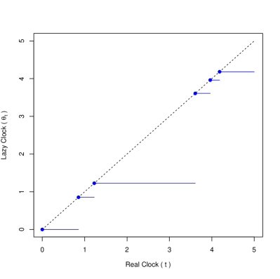
(a) Poisson Lazy clock ($\lambda=3/2$, see Section 3.1.1)

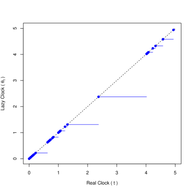
(b) Brownian Lazy clock (see Section 3.1.2)

Figure 1: Sample path of Lazy clocks on $[0,5]$.

In the sense of this definition, Poisson and Compound Poisson processes are examples of subordinators that keep time frozen almost everywhere but are not lazy clocks however as nothing constraints them to reach $t$ if they jump at $t$. Neither are their capped versions as there are some intervals during which $\theta$ cannot jump or grows linearly.

Remark 3.1.

Note that for each $t>0$, the random variable $\theta_{t}$ is a priori not a $(\mathcal{F}_{s},s\geq 0)$-stopping time. In fact, defining

$$C_{t}:=\inf\{s~{};~{}\theta_{s}>t\}$$

then $(C_{t},\,t\geq 0)$ is an increasing family of $\mathbb{F}$-stopping times. Conversely, for every $t\geq 0$, the lazy clock $\theta$ is a family of $(\mathcal{F}_{C_{s}},\,s\geq 0)$-stopping times, see Revuz-Yor [9, Chapter V].

In the following, we shall show that lazy clocks are essentially linked with last passage times, as illustrated in the next proposition.

Proposition 3.

A process $\theta$ is a lazy clock if and only if there exists a càdlàg process $A$ such that the set $\mathcal{Z}:=\{s;\,A_{s^{-}}=0\text{ or }A_{s}=0\}$ has a.s. zero Lebesgue measure and $\theta_{t}=g_{t}$ with

$$g_{t}:=\sup\{s\leq t;\,A_{s^{-}}=0\text{ or }A_{s}=0\}\;.$$

Proof.

If $\theta$ is a lazy clock, then the result is immediate by taking $A_{t}=\theta_{t}-t$ which is càdlàg, and whose set of zeroes coincides with the jumps of $\theta$, hence is countable. Conversely, fix a path $\omega$. Since $A$ is càdlàg, the set $\mathcal{Z}(\omega)=\{s;A_{s^{-}}(\omega)=0\text{ or }A_{s}(\omega)=0\}$ is closed, hence its complementary may be written as a countable union of disjoint intervals. We claim that

$$\mathcal{Z}^{c}(\omega)=\bigcup_{s\geq 0}]g_{s^{-}}(\omega),g_{s}(\omega)[\;.$$ (3.1)

Indeed, observe first that since $s\longmapsto g_{s}(\omega)$ is increasing, its has a countable number of discontinuities, hence the union on the right hand side is countable. Furthermore, the intervals which are not empty are such that $A_{s}(\omega)=0$ or $A_{s^{-}}(\omega)=0$ and $g_{s}(\omega)=s$. In particular, if $s_{1}<s_{2}$ are associated with non empty intervals, then $g_{s_{1}}(\omega)=s_{1}\leq g_{s_{2}^{-}}(\omega)$ which proves that the intervals are disjoint.
Now, let $u\in\mathcal{Z}^{c}(\omega)$. Then $A_{u}(\omega)\neq 0$. Define $d_{u}(\omega)=\inf\{s\geq u,\,A_{s^{-}}(\omega)=0\text{ or }A_{s}(\omega)=0\}$. By right-continuity, $d_{u}(\omega)>u$. We also have $A_{u^{-}}(\omega)\neq 0$ which implies that $g_{u}(\omega)<u$. Therefore, $u\in]g_{u}(\omega),d_{u}(\omega)[$ which is non empty, and this may also be written $u\in]g_{d_{u}^{-}(\omega)}(\omega),\,g_{d_{u}(\omega)}(\omega)[$ which proves the first inclusion. Conversely, it is clear that if $u\in]g_{s^{-}}(\omega),g_{s}(\omega)[$, then $A_{u}(\omega)\neq 0$ and $A_{u^{-}}(\omega)\neq 0$. Otherwise, we would have $u=g_{u}(\omega)\leq g_{s^{-}}(\omega)$ which would be a contradiction. Equality (3.1) is thus proved. Finally, it remains to write :

$$g_{t}=\int_{0}^{g_{t}}1_{\mathcal{Z}}ds+\int_{0}^{g_{t}}1_{\mathcal{Z}^{c}}ds=\sum_{s\leq t}\Delta g_{s}$$

since $\mathcal{Z}$ has zero Lebesgue measure.
∎

We give below examples of lazy clocks admitting simple closed-form distributions.

3.1.1 Poisson Lazy clock

Example 3.1.

Let $(X_{k},k\geq 1)$ be strictly positive random variables and consider the counting process $\left(N_{t}:=\sum_{k=1}^{+\infty}1_{\{\sum_{i=1}^{k}X_{i}\leq t\}},\,t\geq 0\right).$ Then the process $(g_{t}(N),t\geq 0)$ defined as the last jump time of $N$ prior to $t$ or zero if $N$ did not jump by time $t$:

$$g_{t}(N):=\sup\{s\leq t;N_{s}\neq N_{s^{-}}\}=\sum_{k=1}^{+\infty}X_{k}1_{\{\sum_{i=1}^{k}X_{i}\leq t\}}$$ (3.2)

is a lazy clock.

In the case where $N$ is a Poisson process of intensity $\lambda$, i.e. when the r.v.’s $(X_{k},\,k\geq 1)$ are i.i.d. with an exponential distribution of parameter $\lambda$, the law of $g_{t}(N)$ may easily be computed as follows.

Lemma 3.1.

Assume that $N$ is a Poisson process with parameter $\lambda$. Let $t\geq 0$ and $\delta(x)$ be the Dirac density centered at 0. The distribution of $g_{t}(N)$ is given by

$$f_{g_{t}(N)}(s)=e^{-\lambda t}(\delta(s)+\lambda e^{\lambda s})~{}~{},~{}~{}0\leq s\leq t$$ (3.3)

and is zero elsewhere. Hence, the cumulative distribution function is

$$F_{g_{t}(N)}(s)=1_{\{0\leq s\leq t\}}e^{-\lambda(t-s)}+1_{\{s>t\}}$$ (3.4)

and the moments are given by

$$\operatorname{\mathbb{E}}\left[(g_{t}(N))^{k}\right]=\frac{k!}{(-\lambda)^{k}}(1-\operatorname{\textrm{e}}^{-\lambda t})+\sum_{i=0}^{k-1}(-1)^{i}\frac{t^{k-i}k!}{\lambda^{i}(k-i)!}~{}~{},~{}~{}k\in\{1,2,\ldots\}$$ (3.5)

Proof.

This result may be proven adopting a similar strategy as in Propostion 3 of [13], but we shall take here a shorter route. We merely have to show that (i) $\Pr(g_{t}(N)=0)=e^{-\lambda t}$, (ii) $f_{g_{t}(N)}(s)=\lambda e^{-\lambda(t-s)}$ for all $0<s<t$ and (iii) $\Pr(g_{t}(N)\leq s)=1$ if $s\geq t$. The event $\{g_{t}(N)=0\}$ is equivalent to $\{N_{t}=0\}$ whose probability is $e^{-\lambda t}$, proving (i). But $g_{t}(N)\leq t$ $\Pr$-a.s. justifying (iii). The central point is to notice that the stochastic clock synchronizes to the real clock at each jump. When $t>s$, the event $\{g_{t}(N)\leq s\}$ is equivalent to say that no synchronization took place after $s$, i.e. $\{N_{t}=N_{s}\}$, whose probability is $\Pr(N_{t-s}=0)=e^{-\lambda(t-s)}$. Hence, $g_{t}(N)$ has a mixed distribution: it is zero for $s<0$ and $s>t$, has a probability mass of $e^{-\lambda t}$ at $s=0$, and a density part of $\lambda e^{-\lambda(t-s)}$ for $s\in(0,t]$; the proof is complete. ∎

3.1.2 Brownian Lazy clock

Another simple example is given by the last passage time of a Brownian motion to zero, i.e. $(g_{t}^{0}(W),\,t\geq 0)$. The initial value of the process is $g_{0}^{0}(W)=0$ and the density of $g_{t}^{0}(W)$ is given by the Lévy’s arcsine law (see e.g. [8] p.230):

$$f_{g_{t}^{0}(W)}(s)=\frac{1}{\pi\sqrt{s(t-s)}}~{}~{},~{}~{}0<s<t$$ (3.6)

and zero otherwise. It is also possible to consider several extensions, like the last passage time of $W$ at an affine barrier, $\tilde{g}_{t}(W):=\sup\{s\leq t~{};~{}W_{s}=a+bs\}$. The corresponding density expressed in integral form can be found in  [10] but can be further simplified with the help of the standard Normal cumulative distribution function $\Phi$ and $\Phi^{\prime}=\phi$, see [7] :

$$f_{\tilde{g}_{t}(W)}(s)=\frac{\phi\left(\frac{a+bs}{\sqrt{s}}\right)}{\sqrt{s}}\left(\frac{2}{\sqrt{t-s}}\phi\left(b\sqrt{t-s}\right)+2b\Phi\left(b\sqrt{t-s}\right)-b\right)~{}~{},~{}~{}0<s<t\;.$$ (3.7)

Observe that $\tilde{g}_{t}(W)$ is not always well-defined. When $a\neq 0$ indeed, one needs to specify $\tilde{g}_{t}(W)$ in the cases where $W$ never reaches the barrier before $t$. We set, as is usual, $\tilde{g}_{0}(W):=0$. By doing so, $\tilde{g}$ is adapted to the natural filtration of $W$. In contrasts with $g^{0}_{t}(W)$, $\tilde{g}_{t}(W)$ may have a probability mass at zero, corresponding to the probability of $W$ not to reach the affine barrier prior to $t$. Suppose for instance that $a\geq 0$. Then the event $\{\tilde{g}_{t}(W)=0\}$ is equivalent to the event $\{W_{s}<a+bs;\,\forall s\in(0,t]\}$, itself equivalent to $\{\max_{s\in(0,t]}\{W_{s}-bs\}<a\}$. Hence, the probability mass of $\tilde{g}_{t}(W)$ at 0 corresponds to the probability for a Brownian motion with drift $-b$ to stay below the threshold $a$, which is known to be (see e.g. [12] Corollary 7.2.2)

$$\Pr(\tilde{g}_{t}(W)=0)=\Phi\left(\frac{a+bt}{\sqrt{t}}\right)-\operatorname{\textrm{e}}^{-2ab}\Phi\left(\frac{-a+bt}{\sqrt{t}}\right)\;.$$

Observe that this probability vanishes when $a=b=0$. Hence, one can use $g^{0}(W)$ or $\tilde{g}(W)$ as a lazy clock, depending on whether we want $\Pr(\theta_{t}=0)$ to be zero or strictly positive for $t>0$.
The moments of $\tilde{g}_{t}(W)$, $k\in\{1,2,\ldots\}$ read

$$\operatorname{\mathbb{E}}\left[\left(\tilde{g}_{t}(W)\right)^{k}\right]=\frac{\operatorname{\textrm{e}}^{-ab}}{\pi}\int_{0}^{t}\operatorname{\textrm{e}}^{-\frac{b^{2}}{2}u}\int_{0}^{u}\left(\left(k-\frac{1}{2}\right)s^{k-\frac{3}{2}}+\frac{a^{2}}{2}s^{k-\frac{5}{2}}\right)\operatorname{\textrm{e}}^{-\frac{a^{2}}{2s}}\frac{ds}{\sqrt{u-s}}du$$ (3.8)

which, in the $a=0$ case, simplifies to

$$\operatorname{\mathbb{E}}\left[\left(\tilde{g}_{t}(W)\right)^{k}\right]=\frac{\Gamma\left(k+\frac{1}{2}\right)}{\sqrt{\pi}(k-1)!}\int_{0}^{t}u^{k-1}\operatorname{\textrm{e}}^{-\frac{b^{2}}{2}u}du\;.$$ (3.9)

3.1.3 Bessel lazy clock

Lemma 3.2.

Let $R$ denote a Bessel process with index $\nu\in(-1,0)$ started from 0. The probability density of the lazy clock $g_{t}^{0}(R)=\sup\{s\leq t;\,R_{s}=0\}$ is given, for $0<s<t$, by the generalized Arcsine law :

$$f_{g_{t}^{0}(R)}(s)=\frac{1}{\Gamma(|\nu|)\Gamma(1+\nu)}(t-s)^{\nu}s^{-1-\nu}.$$

Its moments are given via the representation of Beta functions :

$$\operatorname{\mathbb{E}}\left[\left(g_{t}^{0}(R)\right)^{k}\right]=\frac{\Gamma(k-\nu)}{\Gamma(k+1)\Gamma(|\nu|)}t^{k}~{}~{},~{}~{}k\in\{1,2,\ldots\}$$ (3.10)

Note that this lazy clock is $1$-self similar.

Proof.

We have, using the Markov property and applying Fubini (see [3]) :

$$\Pr(g_{t}^{0}(R)\leq s) =\operatorname{\mathbb{E}}\left[\Pr_{X_{z}}(T_{0}>t-s)\right]$$

$$=\int_{0}^{+\infty}\frac{2^{\nu}}{y^{2\nu}\Gamma(|\nu|)}\left(\int_{t-s}^{+\infty}u^{\nu-1}e^{-\frac{y^{2}}{2u}}du\right)\frac{y^{2\nu+1}}{2^{\nu}s^{\nu+1}\Gamma(\nu+1)}e^{-\frac{y^{2}}{2s}}dy$$

$$=\frac{1}{\Gamma(|\nu|)\Gamma(\nu+1)}\int_{t-s}^{+\infty}\frac{u^{\nu}s^{-\nu}}{u+s}du$$

$$=\frac{1}{\Gamma(|\nu|)\Gamma(\nu+1)}\int_{\frac{t}{s}-1}^{+\infty}\frac{r^{\nu}}{r+1}dr$$

after the change of variable $u=rs$. The result then follows by differentiation. ∎

3.2 Time-changed martingales with lazy clocks

In this section we consider a martingale $\tilde{Z}$ whose time is changed with an independent lazy clock to obtain a PWC martingale $Z$. We first show that (in most situations) the lazy clock is adapted to the filtration generated by $Z$. This is done by observing that the knowledge of $\theta$ amounts to the knowledge of its jump times, since the size of the jumps are always obtained as a difference with the calendar time. In particular, the properties of the lazy clock allow one to reconstruct the trajectories of $Z$ on $[0,t]$ only from past values of $\tilde{Z}$ and $\theta$; no information about the future (measured according to the real clock) is required. We then provide the resulting distribution when the clock $g(N)$ is governed by Poisson, inhomogeneous Poisson or Cox processes.

Lemma 3.3.

Let $\tilde{Z}$ be a stochastic process independent from the lazy clock $\theta$ and assume that $\forall u\neq v,\;\Pr(\tilde{Z}_{u}=\tilde{Z}_{v})=0$. Then, $\theta$ is adapted to the filtration $(\mathcal{F}^{Z}_{t},\,t\geq 0)$.

Proof.

Observe first that the countable union

$$\mathcal{N}=\bigcup_{s\leq t,\theta_{s}=s}\{Z_{s}=Z_{s^{-}}\}=\bigcup_{s\leq t,\theta_{s}=s}\{\tilde{Z}_{\theta_{s}}=\tilde{Z}_{\theta_{s^{-}}}\}$$

is of measure zero since $\tilde{Z}$ and $\theta$ are independent. This implies that a.s., the sample paths of $\theta$ (both the jump times and the jump sizes) can be recovered from the sample paths of $Z$ up to $\theta_{t}$, hence up to $t$. Indeed, the set of the jump times of $\theta$ on $[0,t]$ is given by $\{s\in[0,t]:\theta_{s}=s\}$. Moreover, the “synchronization events” $\{\theta_{s}=s\}$ coincide with the “jump events” $\{Z_{s}-Z_{{s^{-}}}>0\}$ so that all jump times of $\theta$ are identified by the jumps of $Z$. But $\theta$ is constant between two jumps and jumps to a known value (the calendar time) each time $Z$ jumps, so we have the a.s. representation $\theta_{t}=\sup\{s\leq t;\;Z_{s}\neq Z_{s^{-}}\}$. This means that both $\theta_{t}$ and $\tilde{Z}_{\theta_{t}}$ are revealed in $\mathcal{F}^{Z}_{\theta_{t}}$ and, in particular, $\mathcal{F}^{\theta}_{t}\subseteq\mathcal{F}^{Z}_{\theta_{t}}$. The proof is concluded by noting that $\theta_{t}\leq t$, leading to $\mathcal{F}^{Z}_{\theta_{t}}\subseteq\mathcal{F}^{Z}_{t}$. ∎

Lemma 3.4.

Let $\tilde{Z}$ be a martingale and $N$ an independent Poisson process with intensity $\lambda$. Then $Z_{t}:=\tilde{Z}_{g_{t}(N)}$ is a PWC martingale with same range as $\tilde{Z}$. Its cumulative distribution function is given by :

$$F_{Z_{t}}(z)=\Pr(Z_{t}\leq z)=e^{-\lambda t}\left(1_{\{Z_{0}\leq z\}}+\lambda\int_{0}^{t}F_{\tilde{Z}_{u}}(z)e^{\lambda u}du\right)$$ (3.11)

Proof.

This result is obvious from the independence assumption between $\tilde{Z}$ and $N$ (i.e. $\theta=g(N)$),

$$F_{Z_{t}}(z)=\int_{0}^{\infty}F_{\tilde{Z}_{u}}(z)\Pr(\theta_{t}\in du)\;.$$ (3.12)

∎

A similar result applies to the inhomogeneous Poisson and Cox cases. The proofs are very similar.

Corollary 3.1.

Let $N$ be an inhomogeneous Poisson processes, with (deterministic) intensity $(\lambda(u),u\in[0,T])$ and $\Lambda(t)=\int_{0}^{t}\lambda(u)du$. Then we have :

$$F_{Z_{t}}(z)=e^{-\Lambda(t)}\left(1_{\{Z_{0}\leq z\}}+\int_{0}^{t}\lambda(u)F_{\tilde{Z}_{u}}(z)e^{\Lambda(u)}du\right)$$ (3.13)

In the case where $N$ is an inhomogeneous Poisson process with stochastic intensity (i.e. Cox process) independent from $\tilde{Z}$,

$$F_{Z_{t}}(z)=\left(1_{\{Z_{0}\leq z\}}P(0,t)+\int_{0}^{t}F_{\tilde{Z}_{s}}(z)d_{s}P(s,t)\right)\;,$$ (3.14)

where we have set $P(s,t):=\operatorname{\mathbb{E}}[e^{-(\Lambda_{t}-\Lambda_{s})}]$ with $\Lambda_{t}:=\int_{0}^{t}\lambda_{u}du$ the integrated intensity process.

Proof.

We start from the inhomogeneous Poisson case, set as hazard rate function $\lambda(u)$ for all $u\in[0,T]$ a sample path $\lambda_{u}(\omega)$ of the stochastic intensity and take the expectation, which amounts to replace $\lambda(u)$ by $\lambda_{u}$ (hence $\Lambda(u)$ by $\Lambda_{u}$) and take the expected value of the resulting cumulative distribution function derived above with respect to the intensity paths:

$$F_{Z_{t}}(z) = \operatorname{\mathbb{E}}\left[\operatorname{\mathbb{E}}\left[\Pr(Z_{t}\leq z)|\lambda(u)=\lambda_{u},~{}0\leq u\leq t\right]\right]$$ (3.15)

$$= 1_{\{Z_{0}\leq z\}}\operatorname{\mathbb{E}}\left[e^{-\Lambda_{t}}\right]+\operatorname{\mathbb{E}}\left[\int_{0}^{t}\lambda_{s}F_{\tilde{Z}_{s}}(z)e^{-(\Lambda_{t}-\Lambda_{s})}ds\right]$$ (3.16)

$$= 1_{\{Z_{0}\leq z\}}P(0,t)+\int_{0}^{t}F_{\tilde{Z}_{s}}(z)\operatorname{\mathbb{E}}\left[\lambda_{s}e^{-(\Lambda_{t}-\Lambda_{s})}\right]ds$$ (3.17)

where in the last equality we have used Tonelli’s theorem to exchange the integral and expectation operators when applied to non-negative functions as well as independence between $\lambda$ and $\tilde{Z}$.
From Leibniz rule, $\lambda_{s}e^{-(\Lambda_{t}-\Lambda_{s})}=\frac{d}{ds}e^{-(\Lambda_{t}-\Lambda_{s})}$ so

$$\operatorname{\mathbb{E}}\left[\lambda_{s}e^{-(\Lambda_{t}-\Lambda_{s})}\right]=\frac{d}{ds}\operatorname{\mathbb{E}}\left[e^{-(\Lambda_{t}-\Lambda_{s})}\right]=\frac{d}{ds}P(s,t)\;.$$ (3.18)

∎

Remark 3.2.

Notice that $P(s,t)$ does not correspond to the expectation of $e^{-\int_{s}^{t}\lambda_{u}du}$ conditional upon $\mathcal{F}_{s}$, the filtration generated by $\lambda$ up to $s$ as often the case e.g. in mathematical finance. It is an unconditional expectation that can be evaluated with the help of the tower law. In the specific case where $\lambda$ is an affine process for example, $\operatorname{\mathbb{E}}\left[e^{-\int_{s}^{t}\lambda_{u}du}|\lambda_{s}=x\right]$ takes the form $A(s,t)e^{-B(s,t)x}$ for some deterministic functions $A,~{}B$ so that

$$P(s,t)=\operatorname{\mathbb{E}}\left[e^{-\int_{s}^{t}\lambda_{u}du}\right]=\operatorname{\mathbb{E}}\left[\operatorname{\mathbb{E}}\left[A(s,t)e^{-B(s,t)\lambda_{s}}\right]\right]=A(s,t)\varphi_{\lambda_{s}}(iB(s,t))\;.$$

Example 3.2.

In the case $\lambda$ follows a CIR process, $d\lambda_{t}=k(\theta-\lambda_{t})dt+\sigma\sqrt{\lambda_{t}}dW_{t}$ with $\lambda_{0}>0$ then $\lambda_{s}\sim r_{s}/c_{s}$ with $c_{s}=\nu/(\theta(1-e^{-ks}))$ and $r_{s}$ is a non-central chi-squared random variable with non-centrality parameter $\nu=4k\theta/\sigma^{2}$ and $\kappa=c_{s}\lambda_{0}e^{-ks}$ the degrees of freedom. So, $\varphi_{\lambda_{s}}(u)=\operatorname{\mathbb{E}}[\operatorname{\textrm{e}}^{i(u/c_{s})r_{s}}]=\varphi_{r_{s}}(u/c_{s})$ where $\varphi_{r_{s}}(v)=\frac{1}{(1-2iv)^{\kappa/2}}\exp\left(\frac{\nu iv}{1-2iv}\right)$.

3.3 Some Lazy martingales without independence assumption

We have seen that when $\tilde{Z}$ is a martingale and $\theta$ an independent lazy clock, then $(Z_{t}=\tilde{Z}_{\theta_{t}},\,t\geq 0)$ is a PWC martingale. We now give an example where the lazy time-change $\theta$ is not independent from the latent process $\tilde{Z}$.

Proposition 4.

Let $B$ and $W$ be two Brownian motions with correlated coefficient $\rho$ and $f$ a continuous function. Define the lazy clock :

$$g_{t}^{f}(W):=\sup\{s\leq t,\;W_{s}=f(s)\}\;.$$

Let $h(W)$ be a progressively measurable process with respect to $W$ and assume that there exists a deterministic function $\psi$ such that :

$$\int_{0}^{g_{t}^{f}(W)}h_{u}(W)dW_{u}=\psi(g_{t}^{f}(W))\;.$$

Then, the process $Z_{t}:=\tilde{Z}_{g_{t}^{f}(W)}$ where $\tilde{Z}_{t}:=\int_{0}^{t}h_{u}(W)dB_{u}-\rho\psi(t)$is a PWC martingale.

Proof.

Let $W^{\perp}$ be a Brownian motion independent from $W$ such that $B=\rho W+\sqrt{1-\rho^{2}}\,W^{\perp}$. The time-change yields :

$$\int_{0}^{g_{t}^{f}(W)}h_{u}(W)dB_{u}-\rho\psi(g_{t}^{f}(W)) =\int_{0}^{g_{t}^{f}(W)}h_{u}(W)dB_{u}-\rho\int_{0}^{g_{t}^{f}(W)}h_{u}(W)dW_{u}$$

$$=\sqrt{1-\rho^{2}}\int_{0}^{g_{t}^{f}(W)}h_{u}(B)dW^{\perp}_{u}$$

$$=\sqrt{1-\rho^{2}}W^{\perp}_{\int_{0}^{g_{t}^{f}(W)}h^{2}_{u}(B)du}$$

which is a PWC martingale since $g^{f}(W)$ and $h(B)$ are independent from $W^{\perp}$. ∎

It is interesting to point out here that the latent process $\tilde{Z}$ is, in general, not a martingale (not even a local martingale). It becomes a martingale thanks to the lazy time-change.

Example 3.3.

We give below several examples of application of this proposition.

1. Take $h_{u}=1$. Then, $\psi=f$ and $\left(B_{g_{t}^{f}(W)}-\rho f(g_{t}^{f}(W)),\,t\geq 0\right)$ is a PWC martingale.
   More generally, we may observe from the proof above that if $H$ is a space-time harmonic function (i.e. $(t,z)\rightarrow H(t,z)$ is $\mathcal{C}^{1,2}$ and such that $\frac{\partial H}{\partial t}+\frac{1}{2}\frac{\partial^{2}H}{\partial z^{2}}=0$), then the process

   $$\left(H\left(B_{g_{t}^{f}(W)}-\rho f(g_{t}^{f}(W)),\,(1-\rho^{2})g_{t}^{f}(W)\right),\;t\geq 0\right)$$

   is a PWC martingale.

2. Following the same idea, take $h_{u}(W)=\frac{\partial H}{\partial z}(W_{u},u)$ for some harmonic function $H$. Then

   $$\int_{0}^{g_{t}^{f}(W)}\frac{\partial H}{\partial z}(W_{u},u)dW_{u} =H\left(W_{g_{t}^{f}(W)},g_{t}^{f}(W)\right)-H(0,0)$$

   $$=H\left(f(g_{t}^{f}(W)),g_{t}^{f}(W)\right)-H(0,0)$$

   and the process $\left(\int_{0}^{g_{t}^{f}(W)}\frac{\partial H}{\partial z}(W_{u},u)dB_{u}-\rho H\left(f(g_{t}^{f}(W)),g_{t}^{f}(W)\right),\,t\geq 0\right)$ is a PWC martingale.

3. As a last example, take $f=0$ and $h_{u}=r(L^{0}_{u})$ where $r$ is a $\mathcal{C}^{1}$ function and $L^{0}$ denotes the local time of $W$ at 0. Then, integrating by parts :

   $$\int_{0}^{g_{t}^{f}(W)}r(L^{0}_{u})dW_{u}=r(L_{g_{t}^{f}(W)}^{0})W_{g_{t}^{f}(W)}-\int_{0}^{g_{t}^{f}(W)}W_{u}r^{\prime}(L^{0}_{u})dL^{0}_{u}=0$$

   since the support of $dL^{0}$ is included in $\{u,W_{u}=0\}$. Therefore, the process $\left(\int_{0}^{g_{t}^{f}(W)}r(L^{0}_{u})dB_{u},\,t\geq 0\right)$ is a PWC martingale.

4 Numerical simulations

In this section, we briefly sketch the construction schemes to sample paths of the lazy clocks discussed above. These procedures have been used to generate Fig. 1. Finally, we illustrate sample paths and distributions of a specific martingale in $[0,1]$ time-changed with a Poisson lazy clock.

4.1 Sampling of lazy clock and lazy martingales

By definition, the number of jumps of a lazy clock $\theta$ on $[0,T]$ is countable, but may be infinite. Therefore, except in some specific cases (such as the Poisson lazy clock), an exact simulation is impossible. Using a discretization grid, the simulated trajectories of a lazy clock $\theta$ on $[0,T]$ will take the form

$$\theta_{t}:=\sup\{\tau_{i},\tau_{i}\leq t\}$$

where $\tau_{0}:=0$ and $\tau_{1},\tau_{2},\ldots$ are (some of) the synchronization times of the lazy clock up to time $T$. We can thus focus on the sampling times $\tau_{1},\tau_{2}\ldots$ whose values are no greater than $T$.

Poisson lazy clock

Trajectories of a Poisson lazy clock $\theta_{t}(\omega)=g_{t}(N(\omega))$ on a fixed interval $[0,T]$ are very easy to obtain thanks to the properties of Poisson jump times.

Algorithm 1 (Sampling of a Poisson lazy clock).

1. Draw a sample $n=N_{T}(\omega)$ for the number of jump times of $N$ up to $T$: $N_{T}\sim Poi(\lambda T)$. 2. Draw $n$ i.i.d. samples from a standard uniform $(0,1)$ random variable $u_{i}=U_{i}(\omega)$, $i\in\{1,2,\ldots,n\}$ sorted in increasing order $u_{(1)}\leq u_{(2)}\leq\ldots\leq u_{(n)}$. 3. Set $\tau_{i}:=Tu_{(i)}$ for $i\in\{1,2,\ldots,n\}$.

Brownian lazy clock

Sampling a trajectory for a Brownian lazy clock requires the last zero of a Brownian bridge. This is the purpose of the following lemma.

Lemma 4.1.

Let $W^{x,y,t}$ be a Brownian bridge on $[0,t]\;,t\leq T$, starting at $W_{0}^{x,y,t}=x$ and ending $W_{t}^{x,y,t}=y$, and define its last passage time at 0 :

$$g_{t}(W^{x,y,t}):=\sup\{s\leq t,\;W^{x,y,t}_{s}=0\}.$$

Then, the cumulative distribution function $F(x,y,t;s)$ of $g_{t}(W^{x,y,t})$ is given, for $s\in[0,t]$ by :

$$\Pr(g_{t}(W^{x,y,t})\leq s)=F(x,y,t;s) := 1-\operatorname{\textrm{e}}^{-\frac{xy}{t}}\left(d_{+}(x,y,t;s)+d_{-}(x,y,t;s)\right)\;,$$

$$\text{where }\qquad d_{\pm}(x,y,t;s) := \operatorname{\textrm{e}}^{\frac{\pm|xy|}{t}}\Phi\left(\mp|x|\sqrt{\frac{t-s}{st}}-|y|\sqrt{\frac{s}{t(t-s)}}\right)\;.$$

In particular, the probability that $W^{x,y,t}$ does not hit 0 during $[0,t]$ equals:

$$\Pr(g_{t}(W^{x,y,t})=0)=F(x,y,t;0)=1-e^{-\frac{xy+|xy|}{t}}.$$

Note also the special case when $y=0$ :

$$\Pr(g_{t}(W^{x,0,t})=t)=1.$$

Proof.

Using time reversion and the absolute continuity formula of the Brownian bridge with respect to the free Brownian motion (see Salminen [11]), the density of $g_{t}(W^{x,y,t})$ is given, for $y\neq 0$, by :

$$\Pr(g_{t}(W^{x,y,t})\in ds)=\frac{|y|\sqrt{t}}{\sqrt{2\pi}}e^{\frac{(y-x)^{2}}{2t}}\frac{1}{\sqrt{s}(t-s)^{3/2}}e^{-\frac{x^{2}}{2s}}e^{-\frac{y^{2}}{2(t-s)}}\,ds.$$

Integrating over $[0,t]$, we first deduce that

$$\frac{|y|\sqrt{t}}{\sqrt{2\pi}}\int_{0}^{t}\frac{e^{-\frac{x^{2}}{2s}}}{\sqrt{s}}\frac{e^{-\frac{y^{2}}{2(t-s)}}}{(t-s)^{3/2}}\,ds=\exp\left(\frac{(|y|+|x|)^{2}}{2t}\right).$$ (4.1)

We shall now compute a modified Laplace transform of $F$, and then invert it. Integrating by parts and using (4.1), we deduce that :

$$\lambda\int_{0}^{t}\frac{e^{-\frac{\lambda}{2s}}}{2s^{2}}F(x,y,t;s)ds=e^{-\frac{\lambda}{2t}}-e^{-\frac{\lambda}{2t}}\exp\left(-\frac{xy}{t}-\frac{|y|\sqrt{\lambda+x^{2}}}{t}\right).$$

Observe next that by a change of variable :

$$\lambda\int_{0}^{t}\frac{e^{-\frac{\lambda}{2s}}}{2s^{2}}F(x,y,t;s)ds=\lambda e^{-\frac{\lambda}{2t}}\int_{0}^{+\infty}e^{-\lambda v}F\left(x,y,t;\frac{1}{2v+1/t}\right)dv$$

hence

$$\int_{0}^{+\infty}e^{-\lambda v}F\left(x,y,t;\frac{1}{2v+1/t}\right)dv=\frac{1}{\lambda}-\frac{1}{\lambda}\exp\left(-\frac{xy}{t}-\frac{|y|\sqrt{\lambda+x^{2}}}{t}\right)$$

and the result follows by inverting this Laplace transform thanks to the formulae, for $a>0$ and $b>0$ :

$$\frac{1}{\lambda}\exp\left(-a\sqrt{\lambda+x^{2}}\right)=\frac{a}{2\sqrt{\pi}}\int_{0}^{+\infty}e^{-\lambda v}\int_{0}^{v}e^{-ux^{2}}\frac{1}{u^{3/2}}e^{-\frac{a^{2}}{4u}}du\,dv$$

and

$$\int_{0}^{z}e^{-au-b/u}\frac{du}{u^{3/2}}=\frac{\sqrt{\pi}}{2\sqrt{b}}\left(e^{2\sqrt{ab}}\text{Erfc}\left(\sqrt{\frac{b}{z}}-\sqrt{az}\right)+e^{-2\sqrt{ab}}\text{Erfc}\left(\sqrt{\frac{b}{z}}+\sqrt{az}\right)\right).$$

∎

Simulating a continuous trajectory of a Brownian lazy clock $\theta$ in a perfect way is an impossible task. The reason is that when a Brownian motion reaches zero at a specific time say $s$, it does so infinitely many times on $(s,s+\varepsilon]$ for all $\varepsilon>0$. Consequently, it is impossible to depict such trajectories in a perfect way. Just like for the Brownian motion, one could only hope to sample trajectories on a discrete time grid, where the maximum stepsize provides some control about the approximation, and corresponds to a basic unit of time. By doing so, we disregard the specific jump times of $\theta$, but focus on the supremum of the zeroes of a Brownian motion in these intervals. To do this, we proceed as follows.

Algorithm 2 (Sampling of a Brownian lazy clock).

1. Fix a number of steps $n$ such that time step $\delta=T/n$ corresponds to the desired time unit. 2. Sample a Brownian motion $w=W(\omega)$ on the discrete grid $[0,\delta,2\delta,\ldots,n\delta]$. 3. In each interval $((i-1)\delta,i\delta]$, $i\in\{1,2,\ldots,n\}$, draw a uniform $(0,1)$ random variable $u_{i}=U_{i}(\omega)$ • If $u_{i}<F(w_{(i-1)\delta},w_{i\delta},\delta;0)$ then $w$ does not reach 0 on the interval • Otherwise, set the supremum $g_{i}$ of the last zero of $w$ as the $s$-root of $F(w_{(i-1)\delta},w_{i\delta},\delta;s)-u_{i}$ 4. Identify the $k$ intervals ($1\leq k\leq n$) in which $w$ has a zero, and set $\tau_{j}:=i_{j}\delta+g_{i_{j}}$, $j\in\{1,\ldots,k\}$ where $i_{j}\delta$ is the left bound of the interval.

4.2 Example: $\Phi$-martingale sampled with a Poisson lazy clock

We conclude this note by providing simulations of a PWC martingale in $[0,1]$ (as well as its probability distribution) obtained by sampling the “so-called” $\Phi$-martingale with a Poisson lazy clock. Lazy martingales evolving in $\mathbb{R}$ (resp. $\mathbb{R}^{+}$) can be found in a similar way by considering a Brownian motion $W$ (resp. Doléans-Dade exponential $\mathcal{E}(W)$) as latent process $\tilde{Z}$. The resulting expressions are equally tractable.

Example 4.1 (PWC martingale on $(0,1)$).

Let $N$ be a Poisson process with intensity $\lambda$ and $\tilde{Z}$ be the $\Phi$-martingale [5] with constant diffusion coefficient $\eta$,

$$\tilde{Z}_{t}:=\Phi\left(\Phi^{-1}(Z_{0})e^{\eta^{2}/2t}+\eta\int_{0}^{t}e^{\frac{\eta^{2}}{2}(t-s)}dW_{s}\right)\;.$$ (4.2)

where $\Phi$ denotes as before the standard Normal CDF. Then, the stochastic process $Z$ defined as $Z_{t}:=\tilde{Z}_{g_{t}(N)}$, $t\geq 0$, is a PWC martingale on $(0,1)$ with CDF

$$F_{Z_{t}}(z)=e^{-\lambda t}\left(1_{\{Z_{0}\leq z\}}+\lambda\int_{0}^{t}\Phi\left(\frac{\Phi^{-1}(z)-\Phi^{-1}(Z_{0})e^{\eta^{2}/2u}}{\sqrt{e^{\eta^{2}u}-1}}\right)e^{\lambda u}du\right)\;.$$ (4.3)

Some sample paths for $\tilde{Z}$ and $Z$ are drawn on Fig. 2. Notice that this martingale $\tilde{Z}$ can be simulated without error using the exact solution.

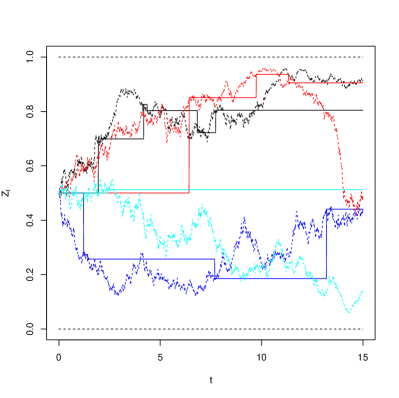
(a) $\eta=25\%$, $\lambda=20\%$

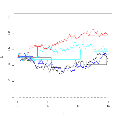
(b) $\eta=15\%$, $\lambda=50\%$

Figure 2: Four sample paths of $\tilde{Z}$ (circles) and $Z$ (no marker) up to $T=15$ years where $\tilde{Z}$ is the $\Phi$-martingale with $Z_{0}=0.5$.

Figure 3 gives the cumulative distribution function of $Z$ and $\tilde{Z}$ where the later is a $\Phi$-martingale. The main differences between these two sets of curves result from the fact that $\Pr(\tilde{Z}_{t}=Z_{0})=0$ for all $t>0$ while $\Pr(Z_{t}=Z_{0})=\Pr(\tilde{Z}_{g_{t}(N)}=Z_{0})=\Pr(N_{t}=0)>0$ and that there is a delay resulting from the fact that $Z_{t}$ correspond to some past value of $\tilde{Z}$.

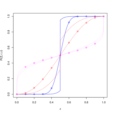
(a) $Z_{0}=50\%$, $\eta=25\%$, $\lambda=20\%$

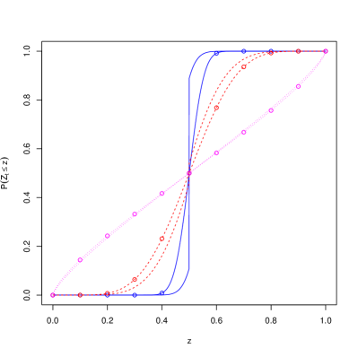
(b) $Z_{0}=50\%$ $\eta=15\%$, $\lambda=50\%$

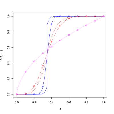
(c) $Z_{0}=35\%$ $\eta=15\%$, $\lambda=50\%$

(d) $Z_{0}=35\%$, $\eta=25\%$, $\lambda=5\%$

Figure 3: Cumulative distribution function of $\tilde{Z}_{t}$ (circles) and $Z_{t}$ (no marker) where $\tilde{Z}$ is the $\Phi$-martingale with initial value $Z_{0}$ and $t$ equals 0.5 (blue solid), 5 (red, dashed) and 40 (magenta, dotted) years.

5 Conclusion and future research

In this paper, we focused on the construction of piecewise constant martingales that is, martingales whose trajectories are piecewise constant. Such processes are indeed good candidates to model the dynamics of conditional expectations of random variables under partial (punctual) information. The time-changed approach proves to be quite powerful: starting with a martingale in a given range, we obtain a PWC martingale by using a piecewise constant time-change process. Among those time-change processes that lazy clocks are specifically appealing: these are time-change processes staying always in arrears to the real clock, and that synchronizes to the calendar time at some random times. This ensures that $\theta_{t}\leq t$ which is a convenient feature when one needs to sample trajectories of the time-change process. Such random times can typically be characterized as last passage times, and enjoy appealing tractability properties. The last jump time of a Poisson process before the current time for instance exhibits a very simple distribution. Other lazy clocks have been proposed as well, based on Brownian motions and Bessel processes, some of which rule out the probability mass at zero. Finally, we provided several martingales time-changed with lazy clocks, called lazy martingales, whose range can be any interval in $\mathbb{R}$ (depending on the range of the latent martingale) and showed that the corresponding distributions can be easily obtained from the law of iterated expectations.

Yet, tractability and even more importantly, the martingale property result from the independence assumption between the latent martingale and the time-change process. In practice however, it might be more realistic to consider cases where the sample frequency (synchronization rate of the lazy clock $\theta$ to the real clock) depends on the level of the latent martingale $Z$. Finding a tractable model allowing for this coupling remains an open question and is the purpose of future research.

References

- [1] J. Bertoin. Lévy processes, volume 121 of Cambridge Tracts in Mathematics. Cambridge University Press, Cambridge, 1996.
- [2] R. Cont and P. Tankov. Financial Modelling with Jump Processes. Chapman & Hall, 2004.
- [3] A. Göing-Jaeschke and M. Yor. A survey and some generalizations of Bessel processes. Bernoulli, 9(2):313–349, 2003.
- [4] I. S. Gradshteyn and I. M. Ryzhik. Table of integrals, series, and products. Elsevier/Academic Press, Amsterdam, seventh edition, 2007.
- [5] M. Jeanblanc and F. Vrins. Conic martingales from stochastic integrals. To appear in Mathematical Finance, 2017.
- [6] M. Jeanblanc, M. Yor, and M. Chesney. Martingale Methods for Financial Markets. Springer Verlag, Berlin, 2007.
- [7] N. Kahale. Analytic crossing probabilities for certain barriers by Brownian motion. Annals of Applied Probability, 18(4):1424–1440, 2008.
- [8] P. Protter. Stochastic Integration and Differential Equations. Springer, Berlin, Second edition, 2005.
- [9] D. Revuz and M. Yor. Continuous martingales and Brownian motion. Springer-Verlag, New-York, 1999.
- [10] P. Salminen. On the first hitting time and the last exit time for a Brownian motion to/from a moving boundary. Advances in Applied Probability, 20:411–426, 1988.
- [11] P. Salminen. On last exit decompositions of linear diffusions. Studia Sci. Math. Hungar., 33(1-3):251–262, 1997.
- [12] S.E. Shreve. Stochastic Calculus for Finance vol. II - Continuous-time models. Springer, 2004.
- [13] F. Vrins. Characteristic function of time-inhomogeneous Lévy-driven Ornstein-Uhlenbeck processes. Statistics and Probability Letters, 116:55–61, 2016.